Compressed Sensing by Shortest-Solution Guided Decimation
Abstract
Compressed sensing is an important problem in many fields of science and engineering. It reconstructs signals by finding sparse solutions to underdetermined linear equations. In this work we propose a deterministic and non-parametric algorithm SSD (Shortest-Solution guided Decimation) to construct support of the sparse solution under the guidance of the dense least-squares solution of the recursively decimated linear equation. The most significant feature of SSD is its insensitivity to correlations in the sampling matrix. Using extensive numerical experiments we show that SSD greatly outperforms -norm based methods, Orthogonal Least Squares, Orthogonal Matching Pursuit, and Approximate Message Passing when the sampling matrix contains strong correlations. This nice property of correlation tolerance makes SSD a versatile and robust tool for different types of real-world signal acquisition tasks.
I Introduction
Real-world signals such as images, voice streams and text documents are highly compressible due to their intrinsic sparsity. Recent intensive efforts from diverse fields (computer science, engineering, mathematics and physics) have established the feasibility of merging data compression with data acquisition to achieve high efficiency of sparse information retrieval Shi-etal-2009 ; Foucart-Rauhut-2013 . This integrated signal processing framework is called compressed sensing or compressed sampling Candes-etal-2006 ; Donoho-2006 ; Gilbert-etal-2002 . At the core of this sampling concept is an underdetermined linear equation involving an real-valued matrix
| (1) |
(Throughout this paper we use uppercase and lowercase bold letters to denote matrices and vectors, respectively.) The column vector is to be determined, while the column vector is the result of sampling operations (measurements) on a hidden signal ; in matrix form, this is
| (2) |
The vector is called a planted solution of (1). Given a matrix and an observed vector , the task is to reconstruct the planted solution .
The sampling process (2) has compression ratio . If the number of non-zero entries in exceeds , some information must be lost in compression and it is then impossible to completely recover from . However, if the sparsity is sufficiently below the compression ratio (), can be faithfully recovered by treating (1) as the sparse representation problem of obtaining a solution with the least number of non-zero entries Donoho-Elad-2003 ; Zhang-etal-2015 .
As -norm minimization is intractable, many different heuristic ideas have instead been explored for this sparse recovery task Shi-etal-2009 ; Zhang-etal-2015 . These empirical methods form three major clusters: greedy deterministic algorithms for -norm minimization, convex relaxations, and physics-inspired message-passing methods for approximate Bayesian inference. Representative and most popular algorithms of these categories are Orthogonal Least Squares (OLS) and Orthogonal Matching Pursuit (OMP) Chen-etal-1989 ; Mallat-Zhang-1993 ; Pati-etal-1993 ; Davis-etal-1994 ; Tropp-2004 ; Tropp-Gilbert-2007 ; Dai-Milenkovic-2009 ; Chatterjee-etal-2012 ; Wang-Li-2017 ; Wen-etal-2017 , -norm based methods Candes-etal-2006 ; Donoho-Elad-2003 ; Gribonval-Nielsen-2003 ; Donoho-2006b ; Tibshirani-1996 ; Chen-etal-2001 , and Approximate Message Passing (AMP) Donoho-Maleki-Montanari-2009 ; Krzakala-etal-2011 , respectively. (In statistical physics the AMP method is known as the Thouless-Anderson-Palmer equation Thouless-Anderson-Palmer-1977 .) To achieve good reconstruction performance, these algorithms generally assume the sampling matrix to have the restricted isometric property (RIP) Candes-Tao-2006 . This requires to be sufficiently random, uncorrelated and incoherent, which is not necessarily easy to meet in real-world applications. In many situations the matrix is intensionally designed to be highly structured. For instance, in the closely related dictionary learning problem often contains several complete sets of orthogonal base vectors to increase the representation capacity, leading to considerable correlations among the columns Donoho-Elad-2003 ; Gribonval-Nielsen-2003 . An efficient and robust algorithm applicable for correlated sampling matrices is highly desirable.
In this work we introduce a simple deterministic algorithm, Shortest-Solution guided Decimation (SSD), that is rather insensitive to the statistical property of the sampling matrix . This algorithm has the same structure as the celebrated OLS and OMP algorithms Chen-etal-1989 ; Mallat-Zhang-1993 ; Pati-etal-1993 ; Davis-etal-1994 ; Tropp-2004 ; Tropp-Gilbert-2007 . It selects a single column of at each iteration step. The most significant difference is on how to choose the matrix columns: While OLS and OMP select the column that having the largest magnitude of (rescaled) inner product with the residual of vector , SSD selects a column under the guidance of the dense least-squares (i.e., shortest Euclidean-length) solution of the decimated linear equation. SSD exploits the left- and right-singular vectors of the decimated sampling matrix.
On random uncorrelated matrices SSD works better than OLS, OMP and -norm based methods; it is slightly worse than AMP which for uncorrelated Gaussian matrices is proven to be Bayes-optimal under correct priors Donoho-Maleki-Montanari-2009 ; Bayati-Montanari-2011 . A major advantage of SSD is that it does not require the sampling matrix to satisfy the RIP condition. Indeed we observe that the performance of SSD on highly correlated matrices remains the same even when -norm based methods, OLS and OMP, and AMP all fail completely. This remarkable feature makes SSD a versatile and robust tool for different types of practical compressed sensing and sparse approximation tasks.
II The general dense solution
When the number of constraints is less than the number of degrees of freedom (), the linear equation (1) has infinitely many solutions and most of them are dense (all the entries of are non-zero). To gain a geometric understanding on the general (dense) solution, we first express the sampling matrix in singular value decomposition (SVD) Golub-Reinsch-1970 as . Here is an orthonormal matrix; is an diagonal matrix whose diagonal elements are the non-negative singular values ; and is an orthonormal matrix. The columns of form a complete set of unit base vectors for the -dimensional real space, so the vectors satisfy . Here and in following discussions denotes the inner product of two vectors and (e.g., ); and is the Kronecker symbol, for and for . Similarly, the orthonormal matrix is formed by a complete set of unit base vectors for the -dimensional real space, with .
Expanding the vector as a linear combination of base vectors , we obtain the following expression for the general solution of (1):
| (3) |
Each of the coefficients is a free parameter that can take any real value; is a column vector uniquely determined by :
| (4) |
where is the Heaviside function, for and for ; is the (Moore-Penrose) pseudo-inverse of Golub-Reinsch-1970 . We call the guidance vector. We will rank the entries of in descending order of their magnitude, and the index of the maximum-magnitude entry of will be referred to as the leading index.
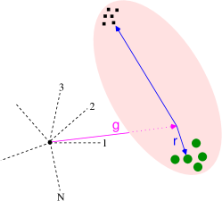
The guidance vector is perpendicular to all the base vectors with . The remainder term of the general solution (3) therefore is perpendicular to . A simple geometric interpretation of (3) is illustrated in Fig. 1: the solution can move freely within the -dimensional subspace (called the null space or kernel of ) spanned by the base vectors with ; this subspace is perpendicular to the guidance vector , which itself is a vector within the -dimensional subspace spanned by the base vectors with .
Notice that the guidance vector is nothing but the shortest Euclidean-length (i.e., least squares) solution Golub-Reinsch-1970 . That is, the -norm achieves the minimum value among all the solutions of (1). This is easily proved by setting all the coefficients of (3) to zero. We may therefore compute by the LQ decomposition method which is more economic than SVD. The sampling matrix is decomposed as , with being an orthonormal matrix (the columns satisfying for ) and being an lower-triangular matrix. The guidance vector is then a linear combination of the unit vectors :
| (5) |
and the coefficient vector is easily fixed by solving the lower-triangular linear equation .
The least-squares solution can also be obtained through convex minimization with the following cost function
| (6) |
where is a column vector of Lagrange multipliers Boyd-etal-2011 . We can employ a simple iterative method of dual ascent:
| (7a) | ||||
| (7b) | ||||
At each iteration step the updating rate parameter is set to an optimal value to minimize the convergence time, see Appendix A for the explicit formula.
III The guidance vector as a cue
The guidance vector is dense and it is not the planted solution we are aiming to reconstruct. But, does the dense bring some reliable clues about the sparse ? Because the observed vector encodes the information of through (2), we see that
| (8) |
Here the matrix is a projection operator:
| (9) |
which projects to the subspace spanned by the first base vectors () of matrix . A diagonal entry of is , while the expression for an off-diagonal entry is .
Notice that, had the summation in (9) included all the base vectors, would have been the identity matrix (), and then would have been identical to . Because only base vectors are included in (9) the non-diagonal entries of no longer vanish, but their magnitudes are still markedly smaller than those of the diagonal entries. Since is a unit vector we may expect that , then we estimate . We may also expect that and are largely independent of each other, then we get that (with roughly equal probability to be positive or negative).
Let us now focus on one entry of . According to (8)
| (10) |
Because is a sparse vector with only non-zero entries, the summation in the above expression () contains only terms. Neglecting the possible weak correlations among the coefficients , we get , where is the rooted square mean value of the non-zero entries of . Notice that does not depend much on the index and it is of the same order as the first term of (10), which is .
For the leading index of , since must have the maximum magnitude among all the entries , we expect that will have the same sign as and it will have considerably large magnitude. It then follows that is very likely to be non-zero and also that .
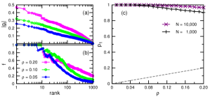
The above theoretical analysis suggests that the vector is very helpful for us to guess which entries of the planted solution have large magnitudes. The validity of this theoretical insight has been confirmed by our numerical simulation results (Fig. 2). We find that indeed the guidance vector contains valuable clues about the non-zero entries of . If an index is ranked on the top with respect to the magnitude of , the corresponding value has a high probability to be non-zero (Fig. 2a and 2b). This is especially true for the leading index of . We also observe that, both for and for , the probability of being non-zero becomes more and more close to unity as the size increases (Fig. 2c). This indicates the cue offered by is more reliable for larger-sized compressed sensing problems.
IV Shortest-Solution guided Decimation (SSD)
Let us denote the sampling matrix as a collection of column vectors , i.e., . With respect to the leading index of the linear equation (1) is rewritten as
| (11) |
Therefore, if all the other entries of the vector are known, is uniquely determined as
| (12) |
Let us denote by the vector formed by deleting from . This vector must satisfy the following linear equation
| (13) |
is an matrix decimated from with its column vectors being
| (14) |
The -dimensional vector is the residual of :
| (15) |
This residual vector and all the decimated column vectors are perpendicular to .
Equation (13) has the identical form as the original linear problem (1). If is a zero vector, we can simply set to be a zero vector too and then a solution with a single non-zero entry is obtained by (12). On the other hand if the residual is non-zero, we can obtain the shortest Euclidean-length (least squares) solution of (13) as the new guidance vector. (If we adopt the dual ascent method (7) for this task, it is desirable to start the iteration from the old guidance vector to save convergence time.) A new leading index (say ) will then be identified, and the corresponding entry is expressed by the remaining entries of as
| (16) |
This Shortest-Solution guided Decimation (SSD) process will terminate within a number of steps (). We will then achieve a unique solution for the selected entries by backtracking the derived equations such as (16) and (12), setting all the other entries of to be exactly zero. This solution will have at most non-zero entries. We provide the pseudo-code of SSD in Algorithm 1 and the corresponding MATLAB code in Appendix B. The longer C++ implementation is provided at power.itp.ac.cn/~zhouhj/codes.html.
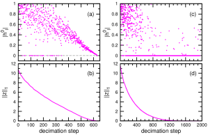
An an illustration, we show in Fig. 3 the traces of two SSD processes obtained on a Gaussian matrix for two planted solutions with non-zero entries. We see that the leading index is not always reliable, sometimes the true value of is actually zero. But the SSD algorithm is robust to these guessing mistakes. As long as the number of such mistakes is relatively small they will all be corrected by the backtrack process of Algorithm 1 (Fig. 3a and 3b). But if these guessing mistakes are too numerous (Fig. 3c and 3d), the backtrack process is unable to correct all of them and the resulting solution will be dense. For Algorithm 1 to be successful, the only requirement is that the indexes of all the non-zero entries of are removed from the working index set in no more than steps. If this condition is satisfied the backtrack process of the algorithm will then completely recover the planted solution .
The SSD algorithm has the same structure as the greedy OLS Chen-etal-1989 and OMP Pati-etal-1993 ; Davis-etal-1994 algorithms. By carefully comparing these three algorithms we realize that they differ only in how to construct the guidance vector . At the beginning of the -th decimation step () the updated sampling matrix has dimension . Then OMP simply sets so the -th entry is , where is the -th column of the current matrix and is the current residual vector. In OLS, is computed by a slightly different expression . In SSD, is the least-squares solution of , so according to (4). After the leading index of is determined, these algorithms then modify and by the same rule (see the two equations in step- of the while loop of Algorithm 1). The total number of arithmetic operations performed in the -th decimation step is approximately for OMP and for OLS; and for SSD this number is approximately if we use repeats of the iteration (7) to update . It may be reasonable to assume , then SSD is roughly – times slower than OMP and OLS. On the other hand, the results in the next section will demonstrate that the guidance vector of SSD is much better than those of OMP and OLS, especially on correlated sampling matrices.
V Comparative results
We now test the performance of SSD on sparse reconstruction tasks involving both uncorrelated and correlated sampling matrices. As the measure of correlations we consider the condition number , which is the ratio between the maximum () and the minimum () singular value of the sampling matrix . An uncorrelated matrix has condition number , while a highly correlated or structured matrix has condition number . Notice that the RIP condition is severely violated for matrices with large values. Two types of sampling matrix are examined in our simulations:
Gaussian: Each entry of the matrix is an identically and independently distributed (i.i.d) random real value drawn from the Gaussian distribution with mean zero and unit variance. Every two different columns and of such a random matrix are almost orthogonal to each other; that is, . The condition number of a Gaussian matrix is close to , and the RIP condition is satisfied.
Correlated: The matrix is obtained as the product of an matrix and a matrix , so . Both and are Gaussian random matrices as described above. As the rank number approaches from above, the entries in the composite matrix are more and more correlated and the condition number increases quickly.
The planted solutions are sparse random vectors with a fraction of non-zero entries. The positions of the non-zero entries are chosen completely at random from the possible positions. Two types of planted solutions (Gaussian or uniform) are employed. The non-zero entries of are i.i.d random real values drawn from the Gaussian distribution with mean zero and unit variance or from the uniform distribution over , for the Gaussian-type and uniform-type , respectively. The relative distance between and the reconstructed solution is defined as
| (17) |
If this relative distance is considerably small (that is, ), we claim that the planted solution has been correctly recovered by the algorithm. We fix the compression ratio to in the numerical experiments. Two different values of are considered, and .
Many heuristic algorithms have been designed to solve the compressed sensing problem. Here we choose four representative algorithms for the comparative study, namely Minimum -norm (ML1), OLS, OMP, and AMP. The algorithm ML1 tries to find a solution of (1) with minimized -norm . Here we use the MATLAB toolbox L1_MAGIC candes2005l1 . The stop criterion for the primal-dual routine of this code is set to be following the literature. The OLS and OMP algorithms are implemented according to Chen-etal-1989 ; Tropp-2004 ; Tropp-Gilbert-2007 . The AMP algorithm is implemented according to Donoho-Maleki-Montanari-2009 ; Krzakala-etal-2011 . The Gauss-Bernoulli prior is assumed for the planted solution in the AMP algorithm as in Donoho-Maleki-Montanari-2009 ; Krzakala-etal-2011 , and the sparsity of is revealed to AMP as input.
V.1 Gaussian sampling matrix
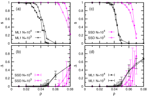
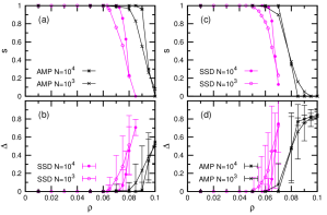
The performance of SSD on Gaussian sampling matrices is compared with those of ML1 (Fig. 4), OLS and OMP (Fig. 5), and AMP (Fig. 6). Our simulation results demonstrate that, at fixed compression ratio the transition between successful and unsuccessful reconstruction becomes sharper as increases. At and , when the planted solutions are Gaussian-type, SSD can successfully reconstruct the planted solutions with high probability (e.g., success rate ) if the signal sparsity is . The corresponding values for ML1, OLS and OMP, and AMP are, respectively, , and . When the planted solutions are uniform-type, SSD can successfully reconstruct at sparsity . The corresponding values for ML1, OLS and OMP, and AMP are, respectively, , and .
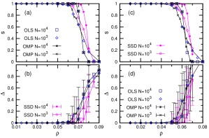
It is encouraging to observe that SSD achieves much better performance than the -norm based ML1. In comparison with ML1, the SSD algorithm is closer to -norm minimization since it tries to find the non-zero entries of but does not care about the magnitude of these entries.
The SSD algorithm slightly outperforms OLS and OMP on the Gaussian matrices. Because the different columns of a Gaussian random matrix are almost orthogonal to each other, the pseudo-inverse does not differ very much from the transpose . This could explain why SSD only weakly improves over OLS and OMP. Similar small improvements of SSD over OLS and OMP are observed on uniform sampling matrices whose entries are i.i.d real values uniformly distributed in . These comparative results suggest that the SSD iteration process makes less guessing mistakes than the OLS and OMP iterations do.
The AMP algorithm performs considerably better than SSD on the Gaussian matrices (Fig. 6). This may not be surprising since AMP is an global optimization approach. Compared with SSD, the AMP algorithm also takes more additional information of as input, including its sparsity level and the probability distribution of its non-zero entries, which may not be available in some real-world applications.
V.2 Correlated sampling matrix
Although SSD in comparison with AMP does not give very impressive results on Gaussian random matrices, it works much better than AMP (and also OLS, OMP and ML1) on correlated matrices. Let us first consider an ill-conditioned matrix instance obtained by multiplying two random Gaussian matrices of size and . The condition number of this matrix is . The message-passing iteration of AMP quickly diverges on this instance and the algorithm then completely fails, even for very small sparsity . Similar divergence problem is experienced for the ML1 algorithm. OLS and OMP have no difficulty in constructing a solution , but their solutions are rather dense and are much different from the planted solution (Fig. 7, cross points). On the other hand, SSD is not affected by the strong correlations of this matrix and it fully reconstructs (Fig. 7, plus points). From Fig. 7 we see that SSD initially causes a smaller decrease in the Euclidean length (-norm) of the signal vector than OMP (or OLS) does, but the slope of decreasing keeps roughly the same in later iterations.
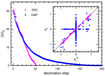
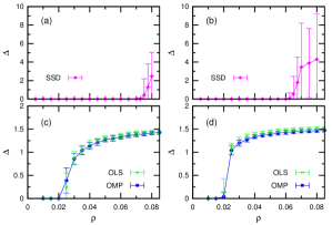
Figure 8 shows how the performances of SSD, OLS and OMP change with the sparsity of the planted solutions on another larger matrix of , , and condition number . (The results of AMP and ML1 are not shown because they always fail to recover .) We observe that OLS and OMP work only for sparsity , while SSD is successful up to sparsity for Gaussian-type and up to for uniform-type . Comparing Fig. 8 with Fig. 5 we see that SSD performs almost equally good on the highly correlated matrix but OLS and OMP are very sensitive to correlations of the matrix.
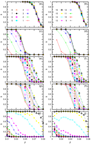
To see how the algorithmic performance is affected by the condition number of the sampling matrices, we generate a set of correlated matrices according to the described protocol using different values of , , , , , , , , , , , , , , , . These matrices are labeled with index ranging from to in Fig. 9 and their corresponding condition numbers are , , , , , , , , , , , , , , and , respectively. We find that SSD is very robust to correlations (Fig. 9a and 9b) but the other algorithms are not: the performances of ML1, OLS and OMP, and AMP all severely deteriorate with the increasing of (Fig. 9c - 9j).
We have also tested the algorithms on correlated matrices generated by some other more complicated protocols. These additional simulation results (not shown here) further confirm the high degree of insensitivity of SSD. This rather peculiar property should be very desirable in practical applications because it greatly relaxes the requirements on the sampling matrix.
VI Conclusion and discussions
In this paper we introduced the Shortest-Solution guided Decimation (SSD) algorithm for the compressed sensing problem and tested it on uncorrelated and correlated sampling matrices. The SSD algorithm is a geometry-inspired deterministic algorithm that does not explicitly try to minimize a cost function. SSD outperforms OLS and OMP in recovering sparse planted solutions; and it is especially competitive in treating highly correlated or structured matrices, on which the tested other representative algorithms (ML1, OLS and OMP, and AMP) all fail.
Mathematical and algorithmic studies Foucart-Rauhut-2013 ; Zhang-etal-2015 on the compressed sensing problem have focused overwhelmingly on uncorrelated random matrices satisfying the restricted isometric property Candes-Tao-2006 . But the RIP incoherence condition can be severely violated in real-world practical problems (see Otsuki-etal-2017 for an example in physics on quantum Monte Carlo data analysis). Existing algorithms in the literature were not designed for tackling highly correlated sampling matrices, and this challenging issue has begun to be discussed only very recently (see, e.g., the work of Ma-Ping-2017 ; Rangan-etal-2016 on orthogonal AMP). The SSD algorithm is a significant step along this direction. The demonstrated high degree of tolerance to correlations indicates that SSD can serve as a versatile and robust tool for different types of compressed sampling problems and sparse representation/approximation problems.
Rigorous theoretical understanding is largely absent on why the SSD algorithm is highly tolerant to structural correlations in the sampling matrix. We feel that (i) viewing the sparse recovery problem from the angle of eigen-subspace projection (8) and (ii) recursively adjusting this eigen-projection by modifying the matrix and the signal vector are crucial to make SSD insensitive to correlations. We offered some qualitative arguments in Section III, especially through (8) and (10), on why the dense guidance vector is useful to sparse reconstruction. More rigorous theoretical understanding on the SSD process needs to be pursued in the future. It looks quite promising to investigate the performance bound of SSD on ensembles of correlated matrices as a phase transition problem.
In this paper we only considered the ideal noise-free situation; but for practical applications it will be necessary to take into account possible uncertainty in the sampling matrix and the unavoidable measurement noise in the signal vector . SSD is slower than OLS and OMP by a constant factor in terms of time complexity. To further accelerate the SSD process an easy adaptation is to fix a small fraction of the active indices instead of just one of them in each decimation step (see, for example, Wang-Li-2017 ). We also need to extend the SSD algorithm to complex-valued compressed sensing problems.
Appendix A Accelerated dual ascent process
Let us denote by the gap vector after the -th iteration step of the dual ascent process (7), that is
| (18) |
Then after the -th iteration step, we have
| (19a) | ||||
| (19b) | ||||
where the auxiliary column vector is defined as
| (20) |
Notice that the Euclidean length (-norm) of will be minimized by setting
| (21) |
This optimal value of is used in the dual ascent process.
Appendix B MATLAB code
As a simple demo we include here a MATLAB code which realizes the SSD algorithm in the most direct way. This code involves computing the pseudo-inverse of the matrix , so it is not optimal in terms of time complexity. The more efficient implementation based on convex optimization (6) is documented at power.itp.ac.cn/~zhouhj/codes.html.
Acknowledgment
H.J.Z. thanks Jing He, Fengyao Hou and Hongbo Jin for help in computer simulations; P.Z. acknowledges helpful discussions with Dong Liu, Xiangming Meng and Chuang Wang; M.S. acknowledges the hospitality of ITP-CAS during his stay as an intern student. H.J.Z. and P.Z. acknowledge the hospitality of Kavli Institute for Theoretical Sciences (KITS-UCAS) during the workshop “Machine Learning and Many-Body Physics” (June 28–July 7, 2017). This research was supported by the National Natural Science Foundation of China (grant numbers 11421063 and 11647601) and the Chinese Academy of Sciences (grant number QYZDJ-SSW-SYS018). The numerical computations were carried out at the HPC Cluster of ITP-CAS and the Tianhe-2 platform of the National Supercomputer Center in Guangzhou.
References
- (1) G.-M. Shi, D.-H. Liu, D.-H. Gao, Z. Liu, J. Lin, and L.-J. Wang, “Advances in theory and application of compressed sensing,” Acta Electronica Sinica, vol. 37, pp. 1070–1081, 2009.
- (2) S. Foucart and H. Rauhut, A Mathematical Introduction to Compressive Sensing. New York: Springer, 2013.
- (3) E. Candès, J. Romberg, and T. Tao, “Robust uncertainty principles: Exact signal reconstruction from highly incomplete frequency information,” IEEE Trans. Inf. Theory, vol. 52, pp. 489–509, 2006.
- (4) D. L. Donoho, “Compressed sensing,” IEEE Trans. Inf. Theory, vol. 52, pp. 1289–1306, 2006.
- (5) A. C. Gilbert, S. Guha, P. Indyk, S. Muthukrishnan, and M. Strauss, “Near-optimal sparse fourier representations via sampling,” in Proc. 34th Annueal ACM Symposium on Theory of Computing (STOC ’02). Montreal, Quebec, Canada: ACM, New York, 2002, pp. 152–161.
- (6) D. L. Donoho and M. Elad, “Optimally sparse representation in general (nonorthogonal) dictionaries via minimization,” Proc. Ntal. Acad. Sci. USA, vol. 100, pp. 2197–2202, 2003.
- (7) Z. Zhang, Y. Xu, J. Yang, X. Li, and D. Zhang, “A survey of sparse representation: Algorithms and applications,” IEEE Access, vol. 3, pp. 490–530, 2015.
- (8) S. Chen, S. A. Billings, and W. Luo, “Orthogonal least squares methods and their application to non-linear system identification,” Int. J. Control, vol. 50, pp. 1873–1896, 1989.
- (9) S. G. Mallat and Z. Zhang, “Matching pursuits with time-frequency dictionaries,” IEEE Trans. Signal Processing, vol. 41, pp. 3397–3415, 1993.
- (10) Y. C. Pati, R. Rezaiifar, and P. S. Krishnaprasad, “Orthogonal matching pursuit: Recursive function approximation with applications to wavelet decomposition,” in Proc. 27th Asilomar Conference on Signals, Systems and Computers. IEEE, 1993, pp. 40–44.
- (11) G. M. Davis, S. G. Mallat, and Z. Zhang, “Adaptive time-frequency decompositions,” Optical Engineering, vol. 33, pp. 2183–2191, 1994.
- (12) J. A. Tropp, “Greed is good: Algorithmic results for sparse approximation,” IEEE Trans. Inf. Theory, vol. 50, pp. 2231–2242, 2004.
- (13) J. A. Tropp and A. C. Gilbert, “Signal recovery from random measurements via orthogonal matching pursuit,” IEEE Trans. Inf. Theory, vol. 53, pp. 4655–4666, 2007.
- (14) W. Dai and O. Milenkovic, “Subspace pursuit for compressive sensing signal reconstruction,” IEEE Trans. Inf. Theory, vol. 55, pp. 2230–2249, 2009.
- (15) S. Chatterjee, K. V. S. Hari, P. Händel, and M. Skoglund, “Projection-based atom selection in orthogonal matching pursuit for compressive sensing,” in Proceedings of the 2012 National Conference on Communications. Kharagpur, India (3-5 Feb., 2012): IEEE, 2012.
- (16) J. Wang and P. Li, “Recovery of sparse signals using multiple orthogonal least squares,” IEEE Trans. Signal Processing, vol. 65, pp. 2049–2062, 2017.
- (17) J. Wen, J. Wang, and Q. Zhang, “Nearly optimal bounds for orthogonal least squares,” IEEE Trans. Signal Processing, vol. 65, pp. 5347–5356, 2017.
- (18) R. Gribonval and M. Nielsen, “Sparse representations in unions of bases,” IEEE Trans. Inf. Theory, vol. 49, pp. 3320–3325, 2003.
- (19) D. L. Donoho, “For most large underdetermined systems of linear equations the minimal 1-norm solution is also the sparsest solution,” Commun. Pure and Applied Math., vol. 59, pp. 797–829, 2006.
- (20) R. Tibshirani, “Regression shrinkage and selection via the lasso,” J. R. Statist. Soc. B, vol. 58, pp. 267–288, 1996.
- (21) S. S. Chen, D. L. Donoho, and M. A. Saunders, “Atomic decomposition by basis pursuit,” SIAM review, vol. 43, pp. 129–159, 2001.
- (22) D. L. Donoho, A. Maleki, and A. Montanari, “Message-passing algorithms for compressed sensing,” Proc. Natl. Acad. Sci. USA, vol. 106, pp. 18 914–18 919, 2009.
- (23) F. Krzakala, M. Mézard, F. Sausset, Y. F. Sun, and L. Zdeborová, “Statistical-physics-based reconstruction in compressed sensing,” Phys. Rev. X, vol. 2, p. 021005, 2012.
- (24) D. J. Thouless, P. W. Anderson, and R. G. Palmer, “Solution of ‘solvable model of a spin glass’,” Phil. Mag., vol. 35, pp. 593–601, 1977.
- (25) E. J. Candés and T. Tao, “Near optimal signal recovery from random projections: universal encoding strategies?” IEEE Trans. Inf. Theory, vol. 52, pp. 5406–5425, 2006.
- (26) M. Bayati and A. Montanari, “The dynamics of message passing on dense graphs, with applications to compressed sensing,” IEEE Trans. Inf. Theory, vol. 57, pp. 764–785, 2011.
- (27) G. H. Golub and C. Reinsch, “Singular value decomposition and least squares solutions,” Numerische Mathematik, vol. 14, pp. 403–420, 1970.
- (28) S. Boyd, N. Parikh, E. Chu, and B. Peleato, “Distributed optimization and statistical learning via the alternating direction method of multipliers,” Foundations and Trends in Machine Learning, vol. 3, pp. 1–122, 2011.
- (29) E. Candès and J. Romberg, “L1-magic: Recovery of sparse signals via convex programming,” URL: www.acm.caltech.edu/l1magic/downloads/l1magic.pdf, Tech. Rep., 2005.
- (30) J. Otsuki, M. Ohzeki, H. Shinaoka, and K. Yoshimi, “Sparse modeling approach to analytical continuation of imaginary-time quantum monte carlo data,” Phys. Rev. E, vol. 95, p. 061302(R), 2017.
- (31) J. Ma and L. Ping, “Orthogonal amp,” IEEE Access, vol. 5, pp. 2020–2033, 2017.
- (32) S. Rangan, P. Schniter, and A. Fletcher, “Vector approximate message passing,” arXiv:1610.03082, 2016.