Study of the non-linear eddy-current response in a ferromagnetic plate: theoretical analysis for the 2D case

Abstract

The non-linear induction problem in an infinite ferromagnetic pate is studied theoretically by means of the truncated region eigenfunction expansion (TREE) for the 2D case. The non-linear formulation is linearised using a fixed-point iterative scheme, and the solution of the resulting linear problem is constructed in the Fourier domain following the TREE formalism. The calculation is carried out for the steady-state response under harmonic excitation and the harmonic distortion is derived from the obtained spectrum. This article is meant to be the theoretical part of a study, which will be complemented by the corresponding experimental work in a future communication.

1 Introduction

In material characterization applications, the tested specimen is subject to a strong electromagnetic field in order to trigger its non-linear behaviour. The main interest in these techniques relies on the fact that the magnetic properties of ferromagnetic media, especially their hysteretic characteristics, are strongly related to their micro-structure, and hence they provide an indirect link for the assessment of properties like mechanical strength, presence of residual stresses, etc., which are usually accessible through destructive tests or other complicated and expensive techniques.

In case of planar specimens like strips or plates, the two main methods for establishing the excitation field are using air-cored coils, located above or at both sides of the piece, or via a closed magnetic circuit (yoke), which is brought in contact with the specimen interface.

The simulation of the inspection procedure with either methods requires the solution of a non-linear, hysteretic problem. The standard way of treating this problem is via successive linearisation using either the fixed-point method (also known as polarization or Picard-Banach method) or the Newton-Raphson scheme and the application of a numerical technique for the solution of the resulting linear problem at each iteration. Considerable progress has been made the past years in the development of such solvers based on the finite elements method (FEM) [1, 2], the finite integration technique (FIT) [3, 4, 5] or the integral equation approach [6, 7, 8]. The relevant literature is vast, and the above list should be understood only as indicative.

The main inconvenience in using these techniques is that they rely on the application of a volume mesh, with a large number of degrees of freedom (dofs), which results in the repeated inversion of a large (sparse or full, depending on the formulation) system of linear equations. To overcome this drawback, sophisticated techniques using semi-explicit schemes for the minimization of linear system inversions have been proposed [4, 5]. Another approach to cope with the raised computational effort is to resort to hardware acceleration e.g. using parallel and/or GPU adapted implementations [8, 9, 10]. Note here, that especially in the case of the integral equation approach, whose main drawback is related to the limitations in terms of CPU time and memory due to the full matrices involved, the new generation of solvers based on the sparsification techniques with parallel and/or GPU adapted implementations, as the ones mentioned in [9, 10], has allowed the efficient treatment of large, previously intractable problems.

An additional difficulty is linked with the existence of steep field gradients inside the ferromagnetic materials, which raise increased demands in terms of grid resolution, thus reducing the robustness of the solution and making human expertise indispensable in order to assure the validity of the results.

The above mentioned drawbacks can be partly avoided if we are willing to sacrifice the versatility of generic numerical solvers for the favour of more case-dependant modal approaches. Indeed, since the majority of eddy-current inspection/evaluation configurations involve relatively simple geometries that are amenable to semi-analytical solutions, this approach can be a valuable aid to the analysis, owing to the very convenient computational times and the absence of a computational mesh.

In this article, the non-linear eddy-current response of an infinite ferromagnetic plate to two coaxial air-cored cylindrical coils located at its both sides will be studied by means of a modal approach. The considered configuration presents an important practical interest since it stands for one of the two most important experimental set-ups used in material evaluation applications. The present contribution copes with the theoretical analysis of the problem. An experimental study and comparison with the theoretical results presented here will be the subject of a work in prepare.

The developed solution follows the approach of the polarisation technique, that is, the problem is linearised assuming a constant permeability in the ferromagnetic piece, and the unknown magnetic polarisation is determined via fixed-point iterations. The thus resulting linear problem is a multilayer eddy-current problem with a distributed magnetic source exceeding the domain of the ferromagnetic piece, which is treated by means of the truncated region eigenfunctions expansion (TREE) [11, 12]. A simpler version of the proposed approach has been applied for the study of the 1D problem [13].

The paper is organized as follows. First the general scheme for the linearisation of the state equation is presented without any specific reference to the solution method. The treatment of the resulting linear multilayer problem follows in section III. A discussion on the numerical issues arising from both the modal solution and the application of the non-linear operator is presented in section IV. The results of the proposed method are then compared with the ones obtained via a FIT implementation in time domain based on implicit Euler scheme.

Only the case of harmonic excitation is considered in this work. The article follows the idea of developing the solution in a series of the first harmonics and treating each harmonic separately in the frequency domain [2, 7, 8]. The more general case of the transient response calculation for finite duration (finite energy) signals needs a different treatment, and will be studied in a future work.

2 The non-linear formulation

2.1 Problem statement

Let us consider an infinite ferromagnetic plate of thickness $d$ excited by a pair of coaxial coils whose axis is normal to the plate as shown in Fig. 1. The two coils are located at the two opposite sides of the plate, and they are fed with opposite currents of the same amplitude. This specific excitation mode creates a strong, nearly stationary, tangential magnetic field inside the plate, thus maximizing the magnetization effects inside the material. Using the common practice when dealing with symmetrical configurations, only the upper half of the geometry needs to be considered, the anti-symmetry of the induced eddy-current flow being imposed via a perfectly conducting electric boundary condition (PEC) passing from the middle of the plate as shown in Fig. 1b. The solution to a problem with the given symmetry is referred to in the literature as odd-parity solution [12]. In the rest of the text, we shall refer to the plate volume as region 1, whereas the air domain above the plane will be named as region 2.

Figure 1: Ferromagnetic plate sandwiched between two coils fed with currents of opposite sign: (a) original configuration and (b) equivalent problem.

The plate has non-zero conductivity $\sigma$, and its magnetic properties are described via the constitutive equation

$$\mathbf{B}=\mu_{0}[\mathbf{H}+\mathbf{M}(\mathbf{H})]$$ (1)

where $\mu_{0}$ is the magnetic permeability of the free space, and $\mathbf{M}$ stands for the magnetization of the material, which comprises the non-linear effects. As analysed in [13], it is often beneficial from the computational point of view to introduce an effective relative permeability $\mu_{r}$ greater than one. Eq. (1) then can be rearranged as follows

$$\mathbf{B}=\mu_{r}\mu_{0}\mathbf{H}+\mu_{0}\left[\mathbf{M}(\mathbf{H})+\left(1-\mu_{r}\right)\mathbf{H}\right].$$ (2)

As it becomes clear from (2), the role of the effective permeability is to adjust the slope of the linear part of the constitutive equation in order to approach the actual slope of the non-linear curve, and hence to improve convergence. The exact value of $\mu_{r}$ is however subject to the constrain $\mu<2\mu_{min}$, $\mu_{min}$ being the minimum of the differential permeability, to assure the stability of the iterative scheme [14]. Practically, the choice of $\mu$ is a compromise between convergence speed and stability of the algorithm. For the rest of the article, the convergence will be considered as guaranteed without further investigation.

We define $\mathbf{I}\left(\mathbf{H}\right):=\mu_{0}\left[\mathbf{M}\left(\mathbf{H}\right)+\left(1-\mu_{r}\right)\mathbf{H}\right]$, which will be referred to as effective magnetic polarization, or simply magnetic polarization, for the rest of the text. For $\mu_{r}=1$ it reduces to the usual definition of the magnetic polarization, which is the magnetization of the material scaled by the magnetic permeability of the free space.

2.2 The governing equation

Problems with rotational symmetry can be scalarised by introducing the magnetic vector potential, defined as

$$\mathbf{B}=\nabla\times\mathbf{A}$$ (3)

and making the following ansatz

$$\mathbf{A}=A\mathbf{e}_{\phi}$$ (4)

where $\mathbf{e}_{\phi}$ is the unit vector along the azimuthal direction.

Upon substitution of (3),(4) into the Maxwell’s equations and taking the constitutive relation (2) into account, we obtain the diffusion equation for the magnetic potential

$$\nabla^{2}A-\mu\sigma\frac{dA}{dt}=\mu_{0}J-\mathbf{e}_{\phi}\cdot\nabla\times\mathbf{I}.$$ (5)

with $\mu=\mu_{r}\mu_{0}$, $J$ being the coil current (which by hypothesis has only azimuthal component) and $\mathbf{I}$ the magnetic polarization defined above.

To simplify the notation, we define the linear differential operator $\mathscr{D}:=\nabla^{2}-\mu\sigma d_{t}$, and the non-linear material operator $\mathscr{I}:=\mathbf{e}_{\phi}\cdot\nabla\times\mathbf{I}\left[\bullet\,\mathbf{e}_{\phi}\right]$, which both act on the scalarised potential $A$. The solution of (5) can be written formally as

$$A=\left[\mathbf{1}-\mathscr{D}^{-1}\mathscr{I}\right]^{-1}\mathscr{D}^{-1}\mu_{0}J.$$ (6)

where $\mathbf{1}$ stands for the unit operator.

The bracketed term is a non-linear operator and as such it cannot be inverted analytically. To evaluate (6) approximately, we develop the bracketed expression in Taylor series

$$A=\left[\mathbf{1}-\mathscr{D}^{-1}\mathscr{I}+\left(\mathscr{D}^{-1}\mathscr{I}\right)^{2}+\ldots\right]\mathscr{D}^{-1}\mu_{0}J.$$ (7)

The expression in (7) is an alternative way of writing the fixed-point iterative scheme. More precisely, the total solution is obtained by successive application of the non-linear operator $\mathscr{D}^{-1}\mathscr{I}$ to the coil response inside the linearised medium, namely

$$A_{i+1}=A_{0}+\mathscr{D}^{-1}\mathscr{I}A_{i}$$ (8)

for $i=0,1,2,\ldots$ and $A_{0}=\mu_{0}\mathscr{D}^{-1}J$.

An important feature of the fixed-point iterative scheme that should be emphasised here is that in contrast from other approaches, like Newton, the uniqueness of the solution, at least in the ideal case, can be proved, under reasonable hypotheses on the behaviour of the magnetic constitutive relationship. The approximate solution, in this case, does not suffer of the local minima that cannot be excluded in other iterative approaches.

In the previous discussion, the general scheme for tackling the non-linear problem has been presented without any specific reference of how to solve $\mu_{0}\mathscr{D}^{-1}J$ and evaluate the expression (8). Indeed, both tasks can be carried out using any established numerical scheme. In the the following paragraphs, we will present a semi-analytical (modal) approach for treating both tasks. The main advantage of this approach is the diagonalisation of the linear operator $\mathscr{D}$, which allows fast computation of the fixed-point iterations.

3 Modal solution of the linearised problem

Only the case of harmonic excitation will be considered in this work, i.e. the time dependency of the coil current is taken equal to $J\left(t\right)=J_{0}\sin\left(i\omega_{0}t\right)$, $\omega_{0}$ being the angular frequency. The frequency is assumed sufficient low in order the quasi-static approximation to be valid.

Due to the non-linearity of the material, the final solution will contain, beside the basic harmonic $\omega_{0}$, all its odd multiples $\omega_{p}=p\omega_{0}$, with $p=1,3,\ldots,\infty$. All the time-dependant physical quantities of the problem are thus given by the sum

$$f\left(\mathbf{r},t\right)=\sum\limits_{p=-\infty}^{\infty}f_{p}\left(\mathbf{r}\right)e^{i\omega_{p}t},\;p=\pm 1,\pm 3,\ldots,\infty$$ (9)

where the development coefficients are given by the integrals

$$f_{p}\left(\mathbf{r}\right)=\frac{1}{T}\int\limits_{-\infty}^{\infty}f\left(\mathbf{r},t\right)e^{-i\omega_{p}t}dt$$ (10)

$T$ being the time period of the signal (equals the period of the excitation signal $\omega_{0}/2\pi$). In practice, the spectrum $f_{p}$ decreases very rapidly with the frequency, and hence only a very small number of harmonics is sufficient to provide an excellent accuracy.

In order to avoid unnecessary notation complexity, the harmonic index $p$ will be dropped henceforth. All following relations are understood as being applied for the $p$th harmonic unless otherwise specified.

3.1 Calculation of the coil response: $\mu_{0}\mathscr{D}^{-1}J$

We seek solution to the linear, odd-parity, eddy-current problem of a cylindrical coil over an infinite plate excited by an harmonic current. This is a typical eddy-current testing situation, whose solution is very well studied in the literature [11, 12]. This section will thus serve as a reminder of the basic results, which will be presented without proof.

Following the common practice of the TREE approach, the computational domain is truncated at $\rho=\rho_{L}$ taking advantage of the diffusive character of the solution. Assuming that the $\rho_{L}$ is sufficiently large in order the electromagnetic field to be negligible, we are free to choose the type of condition at the truncation boundary that is more convenient for the analysis. Let us consider a perfect electric conducting (PEC) condition at the truncation boundary.

The solution for the magnetic potential reads

$$A^{(1)}\left(\rho,z\right)=\sum\limits_{\ell=1}^{\infty}J_{1}\left(\kappa_{\ell}\rho\right)\left[C_{\ell}^{(s)}e^{\kappa_{\ell}z}+D_{\ell}^{(d)}e^{-\kappa_{\ell}z}\right]$$ (11)

in the air region above the plate, and

$$A^{(2)}\left(\rho,z\right)=\sum\limits_{\ell=1}^{\infty}J_{1}\left(\kappa_{\ell}\rho\right)C_{\ell}^{(c)}\sinh\left(v_{\ell}z\right)$$ (12)

inside the plate, with the eigenvalues $\kappa_{\ell}$ being determined by the boundary condition at the truncation surface

$$J_{1}\left(\kappa_{\ell}\rho_{L}\right)=0$$ (13)

and $v_{\ell}$ satisfying the dispersion relation

$$v_{\ell}^{2}=\kappa_{\ell}^{2}+k_{p}^{2}.$$ (14)

$k_{p}^{2}$ stands for the dispersion coefficient in the plate and for the $p$th harmonic: $k_{p}^{2}=i\omega_{p}\mu\sigma$. Notice that in air $k_{p}^{2}=0$, which yields $v_{\ell}=\kappa_{\ell}$.

$C_{\ell}^{(s)}$ are the development coefficients for the solution of the coil in the absence of the plate, and they depend only upon the coil geometry and the excitation current. Their expression for the air region between the coil and the plate are given by

$$C_{\ell}^{(s)} =-4\mu_{0}\iota_{0}\sinh\left(\frac{\kappa_{n}l}{2}\right)\frac{\chi\left(\kappa_{n}\rho_{in},\kappa_{n}\rho_{out}\right)}{\kappa_{n}^{5}\left[\rho_{L}J_{1}\left(\kappa_{n}\rho_{L}\right)\right]^{2}}$$

$$\times J_{m}\left(\kappa_{n}\rho_{0}\right)e^{-\kappa_{n}z_{0}}$$ (15)

where $\rho_{in,out}$ stand for the coil inner and outer radius, respectively, $l$ is the coil thickness, and $\iota_{0}$ is the current density across its cross-section. The $\chi$ function stems from the integration over the coil cross-section and it has a closed-form expression in terms of Struve functions $\mathbf{H}_{n}\left(x\right)$: $\chi\left(x_{1},x_{2}\right)=\frac{\pi}{2}[xJ_{0}\left(x\right)\mathbf{H}_{1}\left(x\right)-xJ_{1}\left(x\right)\mathbf{H}_{0}\left(x\right)]_{x_{1}}^{x_{2}}$.

The expressions for the reflection and transmission coefficients $D_{\ell}^{(d)}$ and $C_{\ell}^{(c)}$ read

$$D_{\ell}^{(d)}=\frac{2\mu_{r}\kappa_{\ell}}{\mu_{r}\kappa_{\ell}\sinh\left(v_{\ell}d/2\right)+v_{\ell}\cosh\left(v_{\ell}d/2\right)}e^{\kappa_{\ell}d/2}C_{\ell}^{(s)}$$ (16)

and

$$C_{\ell}^{(c)}=\frac{\mu_{r}\kappa_{\ell}\sinh\left(v_{\ell}d/2\right)-v_{\ell}\cosh\left(v_{\ell}d/2\right)}{\mu_{r}\kappa_{\ell}\sinh\left(v_{\ell}d/2\right)+v_{\ell}\cosh\left(v_{\ell}d/2\right)}e^{\kappa_{\ell}d/2}C_{\ell}^{(s)}$$ (17)

respectively.

3.2 Solution of the update equation: $\mathscr{D}^{-1}\mathscr{I}A_{i}$

Our task here is to calculate the potential solution at the $(i+1)$th iteration, assuming that the magnetic polarization is given (its value is obtained by applying the material operator to the solution of the previous iteration). Formally speaking, we deal with the solution of the inhomogeneous Helmholtz equation, where the support of the right hand side (excitation) term is restricted to the domain of the plate:

$$\left(\nabla^{2}-k_{p}^{2}\right)\Delta A_{i+1}=-\mathbf{e}_{\phi}\cdot\nabla\times\mathbf{I}_{i}$$ (18)

where $\Delta A_{i+1}=A_{i+1}-A_{0}$. The solution of (18) in the interior of the plate can be expanded in two, mutually orthogonal, vector spaces

$$\Delta A^{(2)}=\sum\limits_{\ell,n}c_{\ell n}u_{\ell n}+\sum\limits_{\ell}C_{\ell}^{(I)}U_{\ell}$$ (19)

which span the image and the kernel of the differential operator $\mathscr{D}$ respectively, i.e. it is $\mathrm{span}\{u_{\ell n}\}=\mathrm{im}\left[\mathscr{D}\right]$ and $\mathrm{span}\{U_{n}\}=\ker\left[\mathscr{D}\right]$, with $\mathrm{im}\left[\mathscr{D}\right]\perp\ker\left[\mathscr{D}\right]$ (the double index for the image subspace stems from the two dimensions of the image space). Differently stated, $u_{\ell n}$ yields a special solution for the non-homogeneous equation, whereas $U_{n}$ assures the uniqueness of the total solution according to Fredholm’s alternative theorem. Indeed, $u_{\ell n}$ will introduce a discontinuity at the plate interface, which will be revealed by $U_{n}$ as it will be shown below.

A convenient choice for $u_{\ell n}$ and $U_{n}$ bases for the expansion of the solution is the eigenfunction basis of the Helmholtz operator, which for the given symmetry reads

$$u_{\ell n}\left(\rho,z\right)=J_{1}\left(\kappa_{\ell}\rho\right)\left\{\begin{array}[]{ll}z,&n=0\\ \sin\left(\alpha_{n}z\right),&n=1,2,\ldots,\infty\end{array}\right.$$ (20)

for the image subspace, and

$$U_{\ell}\left(\rho,z\right)=J_{1}\left(\kappa_{\ell}\rho\right)\sinh\left(v_{\ell}z\right)$$ (21)

for the kernel subspace, where $\kappa_{\ell}$ and $v_{\ell}$ are the same eigenvalues with the ones considered for the calculation of the coil response (since we deal with the same boundary conditions), and the are thus given by (13) and (14), respectivelly. The values of $\alpha_{n}$ depend upon the condition at the plate interface $z=d/2$, which is taken to be of PEC-type (again an arbitrary choice). Together with the zero order term $z$, they establish the basis completeness. The PEC condition yields for $\alpha_{n}$

$$\alpha_{n}=2n\pi/d$$ (22)

with $n=1,2,\ldots,\infty$.

We need now to determine the development coefficients $c_{\ell n}$ and $C_{\ell}^{(I)}$. Substitution of (19) upon the Helmholtz equation (18) yields

$$\sum\limits_{\ell=1}^{\infty}\sum\limits_{n=0}^{\infty}\left(\kappa_{\ell}^{2}+\alpha_{n}^{2}+k_{p}^{2}\right)c_{\ell n}u_{\ell n}\left(\rho,z\right)=\mathbf{e}_{\phi}\cdot\nabla\times\mathbf{I}$$ (23)

with $\alpha_{0}=0$. Observing (23) at $z=d/2$, and taking into account the orthogonality of the basis, we obtain the first relation for the zero-order $c_{\ell 0}$ coefficients

$$\left(\kappa_{\ell}^{2}+k_{p}^{2}\right)c_{\ell 0}=\frac{2}{E^{2}}\langle u_{\ell 0}\left(\rho,d/2\right),\mathbf{e}_{\phi}\cdot\nabla\times\mathbf{I}\rangle_{z=d/2}$$ (24)

where $\langle\bullet,\bullet\rangle_{z=d/2}$ denotes the inner product for the radial part of $u_{\ell 0}$, namely

$$\langle f,g\rangle_{z=d/2}:=\int\limits_{0}^{\rho_{L}}\rho f\left(\rho\right)g\left(\rho\right)d\rho$$ (25)

and $E=\rho_{L}J_{0}\left(\kappa_{\ell}\rho_{L}\right)$ is the normalization coefficient of the Bessel function basis.

The remaining coefficients ($n\neq 0$) are obtained by considering the volume of the plate, i.e.

$$\left(\kappa_{\ell}^{2}+\alpha_{n}^{2}+k_{p}^{2}\right)c_{\ell n} =\frac{4}{E^{2}d}\langle u_{\ell n}\left(\rho,z\right),\mathbf{e}_{\phi}\cdot\nabla\times\mathbf{I}\rangle$$

$$-\frac{4}{E^{2}d}c_{\ell 0}\langle u_{\ell n}\left(\rho,z\right),z\rangle$$ (26)

with the inner product $\langle\bullet,\bullet\rangle$ defined as

$$\langle f,g\rangle:=\int\limits_{0}^{\rho_{L}}\int\limits_{0}^{d/2}\rho f\left(\rho,z\right)g\left(\rho,z\right)d\rho dz.$$ (27)

Both (24) and (26) involve spatial derivatives of the magnetic polarization, which is obtained after application of the non-linear material operator to the magnetic field solution of the previous step. Practically, $\mathbf{I}$ is evaluated at a finite number of grid points, and the integrals of the (24),(26) must then be computed numerically. It is thus more convenient from the computational point of view to pass the curl operator on the left side of the inner products and perform the derivations analytically. This is possible thanks to the hermiticity of the curl operator. It can be shown after some standard manipulations that (24),(26) reduce to

$$c_{\ell 0} =\frac{2}{\lambda_{\ell 0}^{2}E^{2}}\int\limits_{0}^{\rho_{L}}\rho J_{1}\left(\kappa_{\ell}\rho\right)\partial_{z}\left[I_{\rho}\left(\rho,z\right)\right]_{z=d/2}d\rho$$

$$+\frac{2}{\lambda_{\ell 0}^{2}E^{2}}\int\limits_{0}^{\rho_{L}}\kappa_{\ell}J_{0}\left(\kappa_{\ell}\rho\right)I_{z}\left(\rho,d/2\right)d\rho$$ (28)

for the $n=0$ coefficients, and

$$c_{\ell n} =-\frac{8\alpha_{n}}{\lambda_{\ell n}^{2}E^{2}d}\int\limits_{0}^{\rho_{L}}\rho J_{1}\left(\kappa_{\ell}\rho\right)d\rho\int\limits_{0}^{d/2}\cos\left(\alpha_{n}z\right)I_{\rho}\left(\rho,z\right)dz$$

$$+\frac{8\kappa_{\ell}}{\lambda_{\ell n}^{2}E^{2}d}\int\limits_{0}^{\rho_{L}}\rho J_{0}\left(\kappa_{\ell}\rho\right)d\rho\int\limits_{0}^{d/2}\sin\left(\alpha_{n}z\right)I_{z}\left(\rho,z\right)dz$$

$$+\frac{4\lambda_{\ell 0}^{2}}{\lambda_{\ell n}^{2}d^{2}\alpha_{n}}\left[1-(-1)^{n}\right]c_{\ell 0}$$ (29)

for $n\neq 0$. In the above relations we have set $\lambda_{\ell n}^{2}=\kappa_{\ell}^{2}+\alpha_{n}^{2}+k_{p}^{2}$. $I_{\rho}$ and $I_{z}$ stand for the radial and axial component of the magnetic polarization respectively. The derivative $\partial_{z}I_{\rho}$ in (28) cannot be reduced any further and has to be evaluated numerically.

To calculate the homogeneous solution and finalize the construction of the total solution, we also need to express the potential in the air region, due to the magnetic polarization of the plate. The general expression will be identical with the one for the coil response, which for the sake of completeness we rewrite here

$$\Delta A^{(1)}\left(\rho,z\right)=\sum\limits_{\ell=1}^{\infty}D_{\ell}^{(I)}J_{1}\left(\kappa_{\ell}\rho\right)e^{-v_{\ell}z}.$$ (30)

Application of the continuity relations for $H_{\rho}$ and $B_{z}$ at the plate interface leads to the following linear system of equations

$$-\mu_{r}\kappa_{\ell}D_{\ell}^{(I)}e^{-\kappa_{\ell}d/2}=v_{\ell}C_{\ell}^{(I)}\cosh\left(v_{\ell}d/2\right)$$

$$+c_{\ell 0}+\sum\limits_{n=1}^{\infty}(-1)^{n}\alpha_{n}c_{\ell n}+\frac{2}{E^{2}}\langle J_{1}\left(\kappa_{\ell}\rho\right),I_{\rho}\left(\rho,z\right)\rangle_{z=d/2}$$ (31)

and

$$D_{\ell}^{(I)}e^{-\kappa_{\ell}d/2}=C_{\ell}^{(I)}\sinh\left(v_{\ell}d/2\right)+c_{\ell 0}d/2.$$ (32)

Eliminating $D_{\ell}^{(I)}$, we obtain the explicit expressions for $C_{\ell}^{(I)}$

$$\left[\mu_{r}\kappa_{\ell}\sinh\left(v_{\ell}d/2\right)+v_{\ell}\cosh\left(v_{\ell}d/2\right)\right]C_{\ell}^{(I)}=$$

$$c_{\ell 0}\left(1+\mu_{r}\kappa_{\ell}d/2\right)+\sum\limits_{n=1}^{\infty}(-1)^{n}\alpha_{n}c_{\ell n}$$

$$+\frac{2}{E^{2}}\langle J_{1}\left(\kappa_{\ell}\rho\right),I_{\rho}\left(\rho,z\right)\rangle_{z=d/2}$$ (33)

whereas the corresponding value for $D_{\ell}^{(I)}$ is obtained directly by (32).

4 Numerical issues

In the above analysis all the sums comprise infinite number of terms. In reality, the numerical evaluation of the solution requires the truncation of both the Fourier spectrum and the modal sums in (11),(12) and (19),(30). This is a common issue in modal techniques, and is exactly the point where the approximation of the method is introduced (it can be seen as the counterpart of the discussion about the mesh in numerical techniques). There is no generally applicable rule (exactly just as there is no general rule of how fixing the mesh). A usually adequate number of modes is of the order of 100-150 per direction. For a more detailed discussion the reader is referred to previous works [15, 16]. The frequency spectrum on the other hand is very rapidly decreasing, which means that the number of harmonics that have to be taken into account is of the order of ten. Notice that due to the point-symmetry of the $B(H)$ curve, only the odd harmonics contribute to the spectrum, a very-well known experimental fact.

As already mentioned in the introduction, the claim that the modal approach is mesh-less is not entirely true in the case of the non-linear problem. In fact, the application of the non-linear operator $\mathscr{I}$ to the field solution has to be carried out in spatial and time domain. This means that the modal solution has to be evaluated numerically at each iteration at a number of discrete points and at specific time samples. However, here we do not deal with a discretisation with the classical sense, since the solution has already been calculated, and hence the applied evaluation mesh has only an indirect impact upon the results. The field has just to be sampled as densely as necessary to adequately describe the spatial and temporal gradients, in the sense of a Nyquist-like criterion. In the context of this work, a uniform orthogonal grid with 1000 points along the radial direction and 100 points along the plate thickness has been used. The temporal discretisation was realized using 800 samples per period. More sophisticated sampling schemes like non-uniform grids or radial basis functions may be considered, yet this is not in the scope of this work.

5 Results

The presented formulation has been applied for the solution of the eddy-current evaluation problem depicted in Fig. 1, with a thin strip of soft-steel taken as specimen. The model results are compared with a reference solution produced using a two-dimensional numerical code based on the FIT method. The numerical solution is calculated directly in the time domain by means of an implicit time-stepping Euler scheme [17].

A convenient steel grade for our validation purposes is the 1010 steel, whose behaviour is with good approximation non-hysteretic. Since it is easier to work with a parametric model instead of the real experimental curve, the Fröhlich-Kennelly model has been used to approximate the material $B(H)$ constitutive relation. It should be noted here that the choice of a particular approximation curve does not affect the validation itself, as long as we are not comparing the theoretical results with measurements. The only plausible constrain is that the considered parametric model must be ”non-linear” enough and present the qualitative characteristics of a real magnetization curve (i.e. steep slope for low fields, saturation for field intensities of the order $\sim$ 1-10 kA/m) in order to demonstrate that the model reproduces correctly the reference results under these conditions. The explicit expression for the Fröhlich-Kennelly model is given by

$$B=\frac{H}{\alpha+\beta|H|}.$$ (34)

The $\alpha$ and $\beta$ parameters are usually chosen in order to best fit the experimental data. In the present example, the Fröhlich-Kennelly model has been fitted using published data for the 1010 steel yielding $\alpha=206.42$ and $\beta=0.59148$. The resulting curve for the given set of parameters is plotted in Fig. 2. The plate conductivity has been set equal to the tabulated experimental value for the given steel grade, namely $\sigma=6.993~{}MS/m$. The strip thickness is $d=2$ mm, which corresponds to a typical thickness of steel strips produced for the auto-mobile industry.

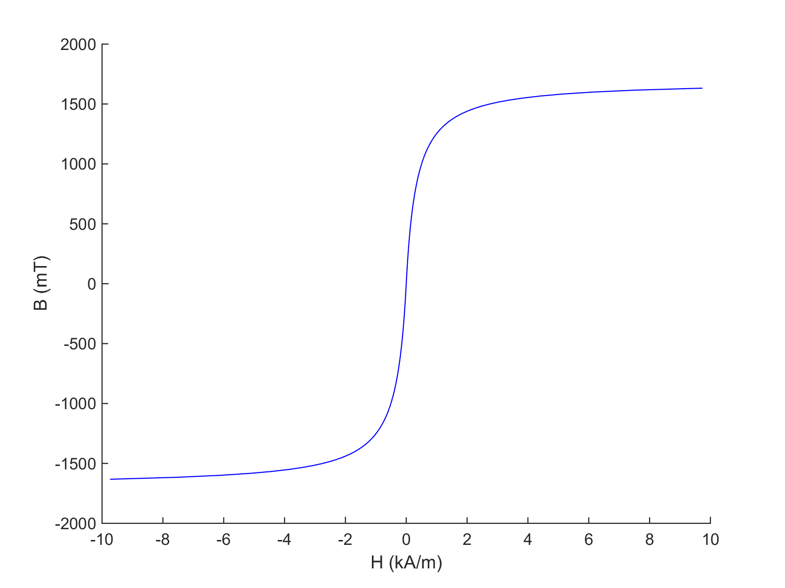
Figure 2: Approximated B-H curve of the 1010 steel.

The two coils are identical with inner and outer radius $\rho_{i}=10$ mm and $\rho_{o}=20$ mm, respectively, length $l=10$ mm, and are wound with 336 turns each. The lift-off is taken equal to $0.5$ mm, i.e. the coils are considered being in contact with the specimen. The working frequency is $60$ Hz.

Given the fact that the modal solution is by construction valid only during the steady-state regime, it is expected that the two results will differ during the transient response of the system. Therefore, the FIT solution is calculated for two periods, and the results are compared only during the second period, where the system has reached the steady-state.

Fig. 3 shows the comparison between modal (TREE) and numerical (FIT) solution for the $B_{\rho}$ and $B_{z}$ variation with the distance from the coils axis at a depth equal to $d/4$ and $t=2$ ms. The two sets of curves correspond to excitation currents of 3 and 10 A.

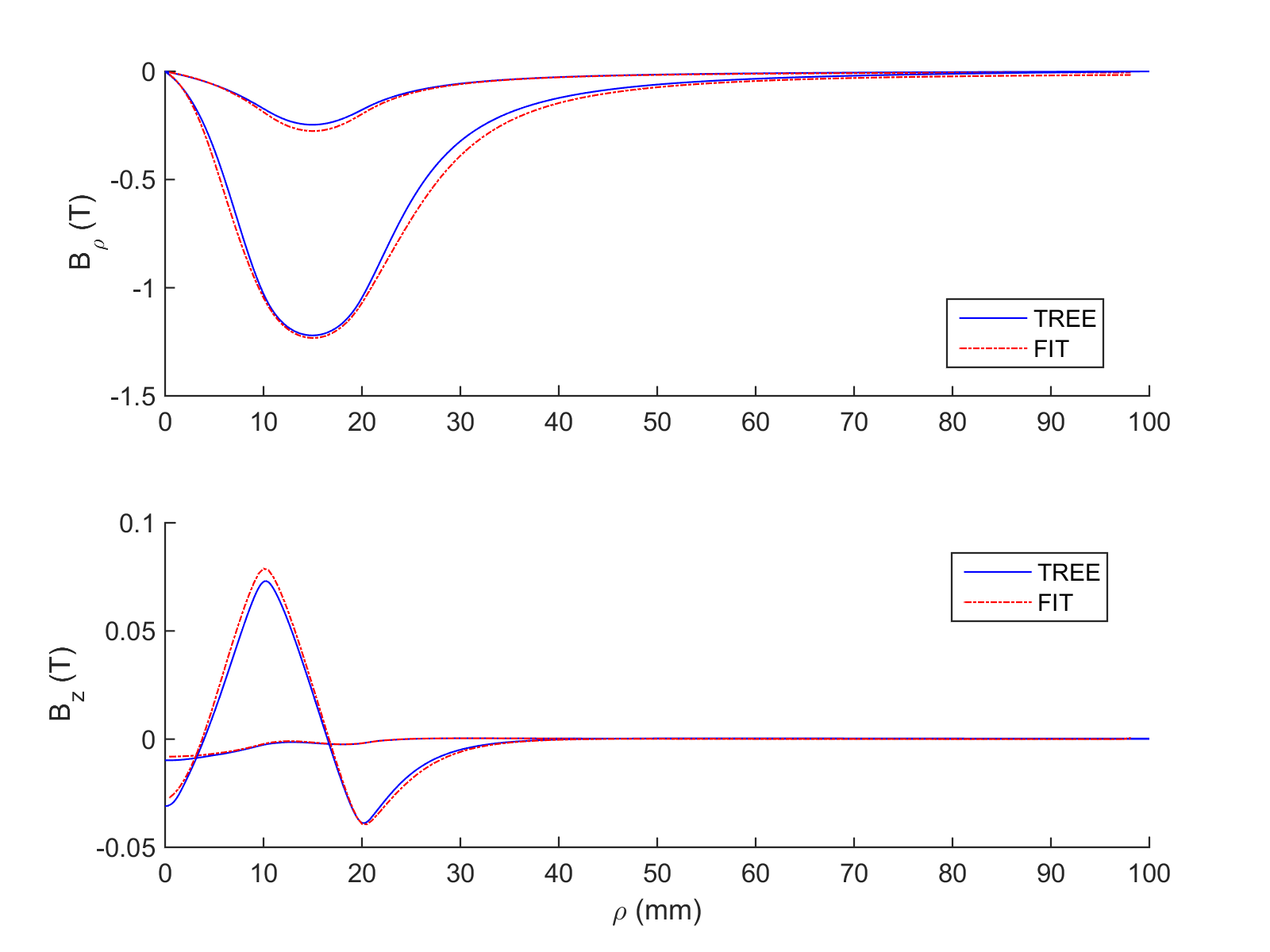
Figure 3: Modal (TREE) vs. numerical (FIT) solution inside the plate as a function of the radial distance and at constant depth (results for 3 and 10 A). The ploted lines correspond to the field values at a given time instance.

The comparison for the temporal variation of both field components at radial distance of $\rho=(\rho_{i}+\rho_{o})/2$ and at the same depth with before ($d/4$) is shown in Fig. 4. The specific observation point has been selected since it is the location where the induced field reaches its maximum amplitude, and hence the non-linear effect becomes more profound (cf. Fig. 3).

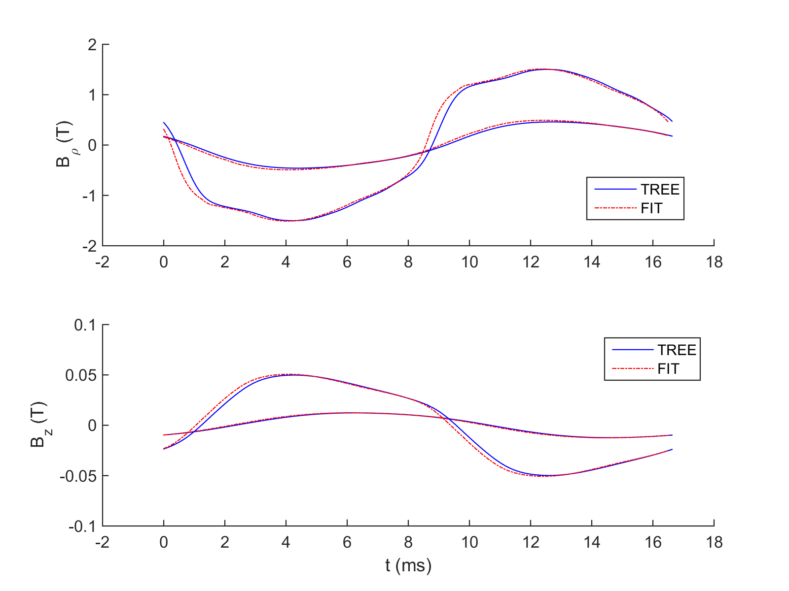
Figure 4: Modal (TREE) vs. numerical (FIT) solution under the coil as a function of time at the point $((\rho_{i}+\rho_{o})/2,\;d/4)$. The two sets of curves correspond to the results obtained for 3 and 10 A.

It is interesting to illustrate the harmonic content of the solution for the selected observation point and calculate the harmonic distortion since it offers a measure of the deviation from the linear regime. It also visualises the contribution from the different harmonics giving feedback where the spectrum can be truncated without loss of information. Finally, the harmonic distortion presents a practical interest since it is one of the more common measurements made by industrial devices of material characterization applications. The comparison of the spectra for the results of the two excitations is shown in Fig. 5.

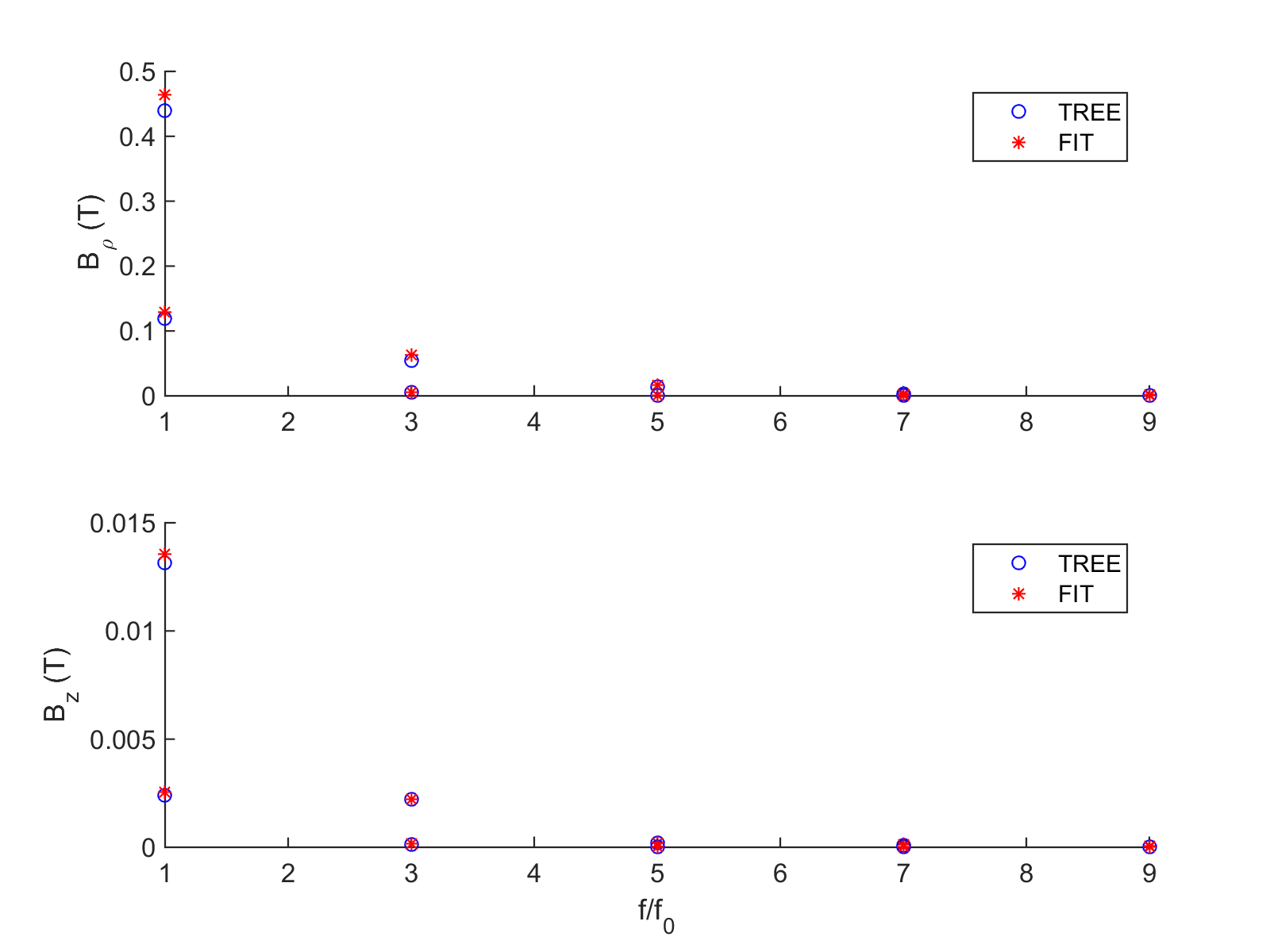
Figure 5: Comparison of the spectra for the modal (TREE) and the numerical (FIT) solution at the point $((\rho_{i}+\rho_{o})/2,\;d/4)$. Results obtained for 3 and 10 A.

A common definition for the harmonic distortion reads

$$K=\sqrt{\frac{\sum_{p=1}^{\infty}A_{2p+1}^{2}}{A_{1}^{2}}}.$$ (35)

where $|A_{p}|$ is the amplitude of the $p$th harmonic. The comparison of the values for the harmonic distortion factor calculated using the modal and the numerical solution for the two components of the magnetic induction at the considered observation point is given in Table 1.

Table 1: Comparison of the harmonic distortion factor calculated using the modal and the numerical solution

	$I=$3A		$I=$10A
	$B_{r}$	$B_{z}$	$B_{r}$	$B_{z}$
TREE	0.042	0.052	0.127	1.169
FIT	0.050	0.070	0.141	1.166

6 Conclusions

The modal approach can be successfully applied to address the non-linear induction problem in ferromagnetic specimens with canonical geometry. If, in addition, the considered piece is infinitely long, e.g. in the case of an infinite multilayer planar or cylindrical specimen, the linearised operator is diagonalisable, which makes the non-linear iterations very cheap.

The presented analysis was restricted to harmonic excitations, and the fact that only a small number of higher harmonics are excited has been exploited for reducing the computational cost. The extension to excitations with periodic (power) signals is straight-forward. The more complex problem of the transient response calculation as well as the response to finite duration (energy) signals, although amenable to similar treatment using Fourier transform, can be more efficiently treated in time or Laplace domain. The corresponding analysis is under way and will be presented in a separate article.

7 Acknowledgement

This work is supported by the CIVAMONT project, aiming at developing scientific collaborations around the NDT simulation platform CIVA developed at CEA LIST.

References

- [1] R. Albanese, G. Rubinacci, Numerical procedures for the solution of nonlinear electromagnetic problems, IEEE Trans. Magn. 28 (2) (1992) 1228–1231.
- [2] O. Bíró, K. Preis, An efficient time domain method for nonlinear periodic eddy current problems, IEEE Trans. Magn. 42 (4) (2006) 695–698.
- [3] S. Drobny, T. Weiland, Numerical calculation of nonlinear transient field problems with the newton-raphson method, IEEE Trans. Magn. 36 (4) (2000) 809–812.
- [4] M. Clemens, S. Schöps, H. D. Gersem, A. Bartel, Decomposition and regularization of nonlinear anisotropic curl-curl DAEs, COMPEL 30 (6) (2011) 1701–1714. doi:10.1108/03321641111168039.
- [5] J. Dutiné, M. Clemens, S. Schöps, G. Wimmer, Explicit time integration of transient eddy current problems, Int. J. Numer. Modell. (2017) jnm.2227–n/adoi:10.1002/jnm.2227.
- [6] R. Albanese, F. I. Hantila, G. Rubinacci, A nonlinear eddy current integral formulation in terms of a two-component current density vector potential, IEEE Trans. Magn. 32 (3) (1996) 784–787.
- [7] I. R. Circ, F. Hantila, An efficient harmonic method for solving nonlinear time-periodic eddy-current problems, IEEE Trans. Magn. 43 (4) (2007) 1185–1188.
- [8] M. d’Aquino, G. Rubinacci, A. Tamburrino, S. Ventre, Three-dimensional computation of magnetic fields in hysteretic media with time-periodic sources, IEEE Trans. Magn. 50 (2) (2014) 53–56.
- [9] S. Börm, -matrix arithmetics in linear complexity, Comput. 77 (2006) 1–28. doi:10.1007/s00607-005-0146-y.
- [10] G. Rubinacci, S. Ventre, F. Villone, Y. Liu, Matrix pencil method for estimating parameters of exponentially damped/undamped sinusoid in noise, J. Comput. Phys. 228 (2009) 1562–1572. doi:10.1016/j.jcp.2008.10.040.
- [11] T. P. Theodoulidis, E. E. Kriezis, Eddy Current Canonical Problems (with applications to nondestructive evaluation), Tech Science Press, Forsyth GA, 2006.
- [12] A. Skarlatos, T. Theodoulidis, Calculation of the eddy-current flow around a cylindrical through-hole in a finite-thickness plate, IEEE Trans. Magn. 51 (9) (2015) 6201507. doi:10.1109/TMAG.2015.2426676.
- [13] A. Skarlatos, T. Theodoulidis, A modal approach for the solution of the non-linear induction problem in ferromagnetic media, IEEE Trans. Magn. 55 (2) (2016) 7000211. doi:10.1109/TMAG.2015.2480043.
- [14] F. I. Hǎnţilǎ, A method of solving stationary magnetic field in non-linear media, Rev. Roum. Sci. Tech.-Électrotechn. et Énerg. 20 (3) (1975) 397–407.
- [15] T. Theodoulidis, J. R. Bowler, Interaction of an eddy-current coil with a right-angled conductive wedge, IEEE Trans. Magn. 46 (4) (2010) 1034–1042. doi:{10.1109/TMAG.2009.2036724}.
- [16] A. Skarlatos, T. Theodoulidis, Solution to the eddy-current induction problem in a conducting half-space with a vertical cylindrical borehole, Proc. R. Soc. London, Ser. A 468 (2142) (2012) 1758–1777. doi:10.1098/rspa.2011.0684.
- [17] M. Clemens, M. Wilke, T. Weiland, Extrapolation strategies in transient magnetic field simulations, IEEE Trans. Magn. 39 (3) (2003) 1171–1174. doi:{10.1109/TMAG.2003.810523}.