(2+1) Regge Calculus:
Discrete Curvatures, Bianchi Identity, and Gauss-Codazzi Equation

Abstract

The first results presented in our article are the clear definitions of both intrinsic and extrinsic discrete curvatures in terms of holonomy and plane-angle representation, a clear relation with their deficit angles, and their clear geometrical interpretations in the first order discrete geometry. The second results are the discrete version of Bianchi identity and Gauss-Codazzi equation, together with their geometrical interpretations. It turns out that the discrete Bianchi identity and Gauss-Codazzi equation, at least in 3-dimension, could be derived from the dihedral angle formula of a tetrahedron, while the dihedral angle relation itself is the spherical law of cosine in disguise. Furthermore, the continuous infinitesimal curvature 2-form, the standard Bianchi identity, and Gauss-Codazzi equation could be recovered in the continuum limit.

I Introduction

The research of quantum gravity, as an attempt to consistently quantize the gravitational field, has been growing fast in many directions. The first step of the modern work in the field was started with the phase-space variables and Hamiltonian of general relativity key-1 ; key-2 . This was done canonically through the construction of a 3-dimensional hypersurface embedded in spacetime, introduced by Arnowitt, Deser, Missner, in the second order formulation of gravity, where the fundamental variable is the 3-dimensional spatial metric key-3 ; key-4 . The quantization of the phase space of gravity was carried directly by Dirac and Bergmann key-5 ; key-6 ; key-7 ; key-8 ; key-9 ; key-10 , resulting in the Wheeler de Witt equation which is difficult to solve key-11 ; key-12 . Other attempt to write gravity in the form similar to Yang-Mills field fibre bundle seems to give a promising path, this is known as the first order formulation, where the fundamental variables are the spatial connection and triads key-13 . The dynamical equations arising from the first order formulation are a set of constraint equations. Attempt to write the constraints first class leads to the definition of the Ashtekar new variables, based on the Plebanski approach key-14 ; key-15 ; key-16 ; key-17 ; key-18 . The use of the new variables leads to a set of solution on the kinematical level; known as the Rovelli-Smolin loop representation key-19 ; key-20 . This in turn gives rise to the field of loop quantum gravity key-21 ; key-22 ; key-23 .

In the fundamental level, loop quantum gravity predicts that space are discrete and fuzzy key-24 ; key-25 ; key-26 . The discreteness is due to the compactness of the $SU(2)$ group, as the gauge group of the 3-dimensional space. The spacetime continuum in the classical general relativity picture is obtained asymptotically in the continuum limit of the theory, where the size and number of grains of space are extremely large key-27 ; key-28 ; key-29 . In between the Plank scale and classical continuous general relativity scale, the mesoscopic scale is defined as the scale where the space behave classically but discrete. This is the scale of the large size and finite numbers of the grains of space, which also known as the semi-classical limit key-30 ; key-31 ; key-32 . The behaviour of spacetime in this scale could be well-approximated by the theory of discrete gravity key-32 .

Discrete gravity had first been studied by Regge, in the second order formulation key-33 ; key-34 . The powerful approach of Regge calculus, which is different from other discrete theories, is in the writing of general relativity formulation without the use of coordinate, i.e., using scalar variables such as angle and norm of area, instead of vectorial variables. Furthermore, it had been shown that discrete gravity will coincide with general relativity in the classical limit, at the level of the action, when the discrete manifold converges to Riemannian manifold key-33 ; key-34 ; key-35 . In the other hand, attempt to write discrete gravity in first order fomulation is done by Barret key-36 .

A part of the theory which is not entirely clear and needs more attention is the ADM splitting in Regge calculus. The ADM formalism is based by an older theorem of Gauss, widely known by mathematicians as the Gauss-Codazzi relation, which describe the relation between curvatures of a manifold with its embeddded submanifold, or, in the language of general relativity, between spacetime and its hypersurface foliation. Works on canonical formulation of Regge calculus had been started by key-37 ; key-38 ; key-39 ; key-40 ; key-41 , and specifically, on the hypersurface foliation and Gauss-Codazzi equation in discrete geometry by key-42 ; key-43 , with the recent works by key-44 ; key-44a . Our work is an attempt to clarify some parts of these previous results.

A complete understanding in the $\left(3+1\right)$ formulation of discrete geometry is needed to understand completely the canonical formulation of quantum gravity, for instance, the evolution of spin-network in loop quantum gravity, and its relation with spinfoam theory. Some problems which are not entirely clear include the procedure to define the hypersurface in the Regge simplicial complex and the relation between the deficit angle as discrete curvature with the curvature 2-form in the first order formulation. Partial results to clarify these issues can be found in key-45 ; key-46 ; key-47 . Another problem which is partially unclear is the definition of extrinsic curvature, which had been studied in key-48 , and more recently in key-49 ; key-50 . The curvatures need to satisfy some geometrical relations, which are, the Bianchi identity and the Gauss-Codazzi relation. The discrete version of the first has been studied extensively, for instance key-51 ; key-52 ; key-53 , and the latter in key-42 ; key-43 ; key-44a , but the discrete geometrical interpretation of these relations remain unclear.

Our work is an attempt to clarify these problem. The first result presented in this article are the clear definitions of both intrinsic and extrinsic discrete curvatures in terms of holonomy and plane-angle representation, a clear relation with their deficit angles, and their clear geometrical interpretations in the first order formulation of discrete geometry. All of these are done with the use of minimal assumptions. The second result is related to the identities and relation between these curvatures. The relation between the Bianchi identity and the law of cosine is already indicated in key-53A . We show that this indication is correct, by obtaining the discrete version of Bianchi identity and its geometrical interpretation. It turns out that the discrete Bianchi identity and Gauss-Codazzi equation, at least in 3-dimension, could be derived from the dihedral angle formula of a tetrahedron, while the dihedral angle relation itself is the spherical law of cosine in disguise. Moreover, we show that the continuous infinitesimal curvature 2-form, the standard Bianchi Identity, and Gauss-Codazzi relation could be recovered in the continuum limit.

The article is structured as follows. In Section II, we reviewed the definition of curvatures in fibre bundle, this include the ADM procedure in the first order formulation. Section III is a brief review of discrete geometry and its formulation in the lattices, which include the definition of the abstract (combinatorial) dual-lattice. Section IV is the main result of out works, which consists the definition of intrinsic curvature 2-form, extrinsic curvature, Bianchi Identity, and Gauss-Codazzi relation in the discrete Regge calculus setting. In Section V, the continuum limit is recovered, altogether with the discussions relevant to our results.

II Curvatures on Fibre Bundle

II.1 The Curvature 2-Form

Suppose we have a standard vector bundle $M\times\mathbb{R}^{n},$ with $M$ is an $n$-dimensional base manifold equipped with a Riemannian metric $g,$ and $\mathbb{R}^{n}$ is the $n$-dimensional vector space. Let $E$ be a fibre bundle locally trivial to $M\times\mathbb{R}^{n}$, equipped with connection $\boldsymbol{A}.$ The $n$-dimensional intrinsic curvature of the connection could be described by the curvature 2-form, which is a map acting on sections of a bundle:

$$\boldsymbol{F}\left(\boldsymbol{s}_{1},\boldsymbol{s}_{2}\right):E_{p} \rightarrow E_{p}$$

$$\boldsymbol{V} \mapsto \boldsymbol{V}^{\prime}.$$

$\boldsymbol{F}\left(\boldsymbol{s}_{1},\boldsymbol{s}_{2}\right)$ is defined as the derivative of the connection:

$$\boldsymbol{F}\left(\boldsymbol{s}_{1},\boldsymbol{s}_{2}\right)\boldsymbol{V}=d_{D}\boldsymbol{A}\>\boldsymbol{V}=\left[D_{\boldsymbol{s}_{1}},D_{\boldsymbol{s}_{2}}\right]\boldsymbol{V}-D_{\left[\boldsymbol{\boldsymbol{s}_{1},\boldsymbol{s}_{2}}\right]}\boldsymbol{V},$$ (1)

with $d_{D}$ is the exterior covariant derivative, $\boldsymbol{s}_{1},\boldsymbol{s}_{2}\in T_{p}M,$ are base space vectors with origin $p\in M,$ and $\boldsymbol{V},\boldsymbol{V}^{\prime}\in E_{p}$ are section of a bundle at $p$. Let $\left\{\partial_{\mu},dx^{\mu}\right\}$ and $\left\{\xi_{I},\xi^{I}\right\}$ respectively, be the local coordinate basis on $M$ and $\mathbb{R}^{n},$ then (1) could be written in a local coordinate of $E_{p}$ as follows:

$$\boldsymbol{F}\left(\partial_{\mu},\partial_{\nu}\right)=\underset{F_{\mu\nu J}^{I}\,\xi_{I}\wedge\xi^{J}}{\underbrace{\partial_{\mu}A_{\nu J}^{I}-\partial_{\nu}A_{\mu J}^{I}+A_{\mu K}^{I}A_{\nu J}^{K}-A_{\nu K}^{I}A_{\mu J}^{K}}}.$$

The curvature 2-form can be geometrically interpreted as an infinitesimal rotation of a test vector $\boldsymbol{V}$ by a rotation bivector (the $\xi^{I}\wedge\xi^{J}$ components, also known as the plane of rotation), if $\boldsymbol{V}$ is parallel-transported around an infinitesimal square loop $\delta\gamma$ of an infinitesimal plane (the $dx^{\mu}\wedge dx^{\nu}$ components) key-54 . It carries the intrinsic property of the curvature of the connection, through a parallel transport of tangent vector around a closed curve, see FIG 1.

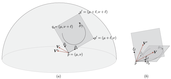
Figure 1: (a). Geometrical interpretation of curvature 2-form. A test vector $\boldsymbol{V}$ is carried around an infinitesimal loop $\delta\gamma$ circling plane $dx^{\mu}\wedge dx^{\nu}$. The resulting vector is $\boldsymbol{V}^{\prime}$, which does not coincide with $\boldsymbol{V}$ if the suface is curved. (b). The rotation bivector and loop orientation in general do not coincide. The test vector $\boldsymbol{V}$ is rotated according to the rotation bivector, with only its component parallel to the plane will get rotated.

$\boldsymbol{F}$ is antisymmetric by the permutation of the base space and section indices:

$$F_{\mu\nu J}^{I}=-F_{\mu\nu I}^{J}=-F_{\nu\mu J}^{I}.$$

If the torsionless condition is satisfied, it satisfies the Bianchi identity:

$$d_{D}\boldsymbol{F}=0,$$ (2)

which states that the second exterior derivative of any general $p$-form $\boldsymbol{\omega}$ is zero:

$$d_{D}^{2}\boldsymbol{\omega}=0.$$

In terms of components, (2) can be written as:

$$d_{D}\boldsymbol{F}=\frac{1}{3!}\left(D_{\mu}F_{\nu\lambda}+D_{\nu}F_{\lambda\mu}+D_{\lambda}F_{\mu\nu}\right)dx^{\mu}\wedge dx^{\nu}\wedge dx^{\lambda}.$$ (3)

Theorem I. The Lie algebra $\mathfrak{so(n)}$ of the rotation group $SO\left(n\right)$ is spanned by antisymmetric tensor.

By Theorem I, for each point $p$ of $E_{p}$, the curvature 2-form carries two planes: the rotation bivector and the loop orientation, where both of them are elements of Lie algebra $\mathfrak{so(n)}$.

Let us consider the components of $\boldsymbol{F}$ for some low-dimensional cases. In dimension two, $\boldsymbol{F}$ has a single non-zero component $F_{xy2}^{1}$ (with its symmetries), written in local coordinate $\left(x,y\right)$ and $\left(1,2\right)$. Therefore, to describe completely the intrinsic curvature of a 2-dimensional surface, one needs a single infinitesimal loop with an $\mathfrak{so(2)}$ algebra attached, on each point of the surface. In dimension three, $\boldsymbol{F}$ has, in general, nine distinct non-zero components (with its symmetries), thus to describe completely a curvature in 3-dimensional space, one needs three infinitesimal loops, with $\mathfrak{so(3)}$ algebras attached on each one of them. Written in coordinates, $F_{xyJ}^{I},$ $F_{yzJ}^{I},$ $F_{zxJ}^{I}$ are $3\times 3$ matrices, elements of $\mathfrak{so(3)}$. Any vector $\boldsymbol{V},$ carried along $\delta\gamma$ circling the $dx\wedge dy$ component of the plane, will be rotated into $\boldsymbol{V}^{\prime}$ by:

$$V^{\prime I}=F_{xyJ}^{I}V^{J}.$$ (4)

$\boldsymbol{F}$ could be defined on a general infinitesimal rectangular loop $\delta\gamma\left(\tau\right)$ circling infinitesimal plane $\boldsymbol{s}_{1}\wedge\boldsymbol{s}_{2}$, with $\boldsymbol{s}_{1}=s_{1}^{\mu}\partial_{\mu}$, as:

$$\boldsymbol{F}\left(\boldsymbol{s}_{1},\boldsymbol{s}_{2}\right)=s_{1}^{\mu}s_{2}^{\nu}F_{\mu\nu J}^{I}\xi_{I}\wedge\xi^{J},$$ (5)

such $\boldsymbol{V}$ carried along $\delta\gamma$, will be rotated into:

$$V^{\prime I} = u^{\mu}v^{\nu}F_{\mu\nu J}^{I}V^{J}.$$

The rotation bivector component $\boldsymbol{F}_{IJ}$ defines a plane of rotation, which are labeled as $\delta\hat{\boldsymbol{J}}$. The ’axis’ of the rotation perpendicular to $\delta\hat{\boldsymbol{J}}$ is labeled as $\star\delta\hat{\boldsymbol{J}}$, where the star $\star$ is used to define the combinatorial (topological) dual of a geometrical quantity; this will be clear in the next section.

The ’axis’ $\star\delta\hat{\boldsymbol{J}}$ is well-defined; we called this, using Regge terminology, as a (infinitesimal) hinge key-33 ; key-34 ; key-55 ; key-57 . The hinge depends on the dimension of the space; if the dimension of space is $n$, then the hinges are $\left(n-2\right)$ forms. This way of viewing the curvature 2-form as pair of planes is important when one consider the curvatures in Regge calculus.

II.2 Gauss-Codazzi Equation in Fibre Bundle

This subsection contains a brief review of Gauss-Codazzi equation, which describe the relation between the curvatures of a manifold with its submanifold. The original Gauss-Codazzi equation is defined on manifold, where, using terminology in general relativity, it is written in a second order formulation. Nevertheless, the concept can be adopted to fibre bundles, such that the Gauss-Codazzi equation can be written in the first order formulation.

The $(n+1)$ split of the fibre bundle of gravity can be done quite similarly to the fibre bundle of a Yang-Mills field, say $E\sim M\times\mathcal{F}$. In Yang-Mills theory, one splits the spacetime $M\sim\mathbb{R}\times\Sigma$ to obtain the electric and magnetic part of the curvature of the fibre, say, $\boldsymbol{E}\wedge dt$ and $\boldsymbol{B}$, which are the curvatures projected on $\mathbb{R}$ and $\Sigma$, respectively. The main difference is, in the Yang-Mills field, one does not split the fibre, because Yang-Mills theory is background-dependent. In the other hand, gravity is a background independent theory where the field and spacetime are indistinguishable entities key-21 ; key-22 . Therefore, spliting the base space will induce the spliting on the fibre.

Let $e$ be a local trivialization, a diffeomorphism map between the trivial vector bundle $M\times\mathbb{R}^{n}$ and the tangent bundle over $M$: $E\sim TM=\cup_{p}\left\{p\times T_{p}M\right\}$. Instead of spliting the base space, one starts with spliting the fibre (which is easier). Let $\xi^{I},$ $I=0,1,2,..,$ be a local coordinate on $\mathbb{R}^{n}.$ The next step is to construct an embedded $n$-dimensional hypersurface $\Sigma\subset M$ by selecting $\xi^{0}$ as a normal to, also, an $n$-dimensional hypersurface $\Omega\subset\mathbb{R}^{n}$. The diffeomorphism $e$ will sends normals $\xi^{0}\in\mathcal{F}\sim\mathbb{R}^{n}$ to $e^{0}=e\left(\xi^{0}\right)\in T_{p}M.$ Then the $(n+1)$ split generated by the normal $\xi^{0}$ on vector space $\mathbb{R}^{n}$ will induce split on $T_{p}M$ generated by $e^{0}=e\left(\xi^{0}\right).$

The following derivation will be based on our previous work key-44a ; $e^{0}$ in general will be a linear combination of coordinate basis vector in $T_{p}M$:

$$e^{0}=e_{\mu}^{0}dx^{\mu}=\underset{N}{\underbrace{e_{0}^{0}}}dx^{0}+\underset{N_{i}}{\underbrace{e_{i}^{0}}}dx^{i},$$

with $N$ and $N_{i}$ are, respectively, the lapse and shift functions. Let us choose a local coordinate in $T_{p}M$ such that:

$$e\left(\xi^{0}\right)=e^{0}=\delta_{\mu}^{0}dx^{\mu}=dx^{0}.$$ (6)

This means one use the time gauge where the lapse $N=1,$ and the shift $N_{i}=0.$

The $n$-dimensional intrinsic curvature of the connection is labeled as:

$$\,{}^{n}\boldsymbol{F}=F_{\mu\nu J}^{I}\xi_{I}\wedge\xi^{J}\otimes dx^{\mu}\wedge dx^{\nu}.$$

In the time gauge, the $(n+1)$ ADM formulation for the curvature 2-form is carried by the spliting $I=0,a,$ and $\mu=0,i$, which are compatible with (6). Therefore, the projection of $\,{}^{n}\boldsymbol{F}$ on $\Sigma$ is:

$$\left.\,{}^{n}\boldsymbol{F}\right|_{\Sigma}=F_{ijb}^{a}\xi_{a}\wedge\xi^{b}\otimes dx^{i}\wedge dx^{j},$$ (7)

written in a local coordinate as:

$$F_{ijb}^{a} = \partial_{i}A_{jb}^{a}-\partial_{j}A_{ib}^{a}+A_{ic}^{a}A_{jb}^{c}-A_{jc}^{a}A_{ib}^{c}+A_{i0}^{a}A_{jb}^{0}-A_{j0}^{a}A_{ib}^{0}.$$

The closed part of $\left.\,{}^{n}\boldsymbol{F}\right|_{\Sigma}$ is clearly the $\left(n-1\right)$-dimensional intrinsic curvature of connection in $\Sigma$, and the rest is the extrinsic curvature part:

$$\,{}^{n-1}\boldsymbol{F} = \,{}^{n-1}F_{ijb}^{a}\xi_{a}\wedge\xi^{b}\otimes dx^{i}\wedge dx^{j}=\left(\partial_{i}A_{jb}^{a}-\partial_{j}A_{ib}^{a}+A_{ic}^{a}A_{jb}^{c}-A_{jc}^{a}A_{ib}^{c}\right)\xi_{a}\wedge\xi^{b}\otimes dx^{i}\wedge dx^{j}$$ (8)

$$\boldsymbol{K} = K_{i}^{a}\xi_{\alpha}\otimes dx^{i}=A_{i0}^{a}\xi_{\alpha}\wedge\xi^{0}\otimes dx^{i}.$$ (9)

As a result, one has the Gauss-Codazzi relation for a fibre bundle of gravity:

$$\left.\,{}^{n}\boldsymbol{F}\right|_{\Sigma}=\,^{n-1}\boldsymbol{F}+\left[\boldsymbol{K},\boldsymbol{K}\right].$$ (10)

The Gauss-Codazzi equation (10) is invariant under coordinate transformation, but it must be kept in mind that the way of writing $\left.\,{}^{n}\boldsymbol{F}\right|_{\Sigma}$, $\,{}^{n-1}\boldsymbol{F}$, and $\boldsymbol{K}$ in (7), (8), and (9) are written in a special gauge condition (6). In a general gauge condition, they do not have such simple forms, for instance, see key-58 .

II.3 Rotations and Holonomies

Another way to describe the curvatures of a manifold is through holonomy. The holonomy $\boldsymbol{H}_{\gamma}\left(\boldsymbol{A},\gamma\left(\tau\right)\right)$ of connection $\boldsymbol{A}$ along a curve $\gamma\left(\tau\right)$ with parameter $\tau$ is defined as a solution to the following equation:

$$D_{\gamma^{\prime}\left(\tau\right)}\boldsymbol{V}\left(\tau\right)=0,\quad\gamma^{\prime}\left(\tau\right)=\frac{d\gamma\left(\tau\right)}{d\tau},\boldsymbol{V}\left(\tau\right)\in T_{p}M,$$

which is:

$$\boldsymbol{V}\left(\tau\right) = \boldsymbol{H}_{\gamma}\left(\boldsymbol{A},\gamma\left(\tau\right)\right)\boldsymbol{V}\left(0\right),$$

$$\boldsymbol{H}_{\gamma}\left(\boldsymbol{A},\gamma\left(\tau\right)\right) = \hat{P}\exp\int_{\gamma\left(\tau\right)}\boldsymbol{A}\left(\gamma\left(\tau\right)\right).$$

$\boldsymbol{A}$ is the spin connection on the fibre bundle $E$, and $\hat{P}$ is the path ordered operator key-21 ; key-22 . It is clear that a holonomy is a subset of the rotation group parallel-transporting vectors while preserving their norms. Its relation with the curvature 2-form can be obtained by considering the holonomy around a closed curve or loop with origin $\mathcal{O}$:

$$\boldsymbol{H}_{\gamma}\left(\boldsymbol{A},\gamma_{\mathcal{O}}\right)=\hat{P}\exp\oint_{\gamma\left(\tau\right)=\partial a}\boldsymbol{A}\left(\gamma\left(\tau\right)\right).$$ (11)

Theorem II (Stokes-Cartan). If $\boldsymbol{\omega}$ is a smooth $\left(n-1\right)$-form with compact support on smooth n-dimensional manifold with boundary $\Omega$, and $\partial\Omega$ labels the boundary of $\Omega$ given the induced orientation, then:

$$\oint_{\partial\Omega}\boldsymbol{\omega}=\int_{\Omega}d_{D}\boldsymbol{\omega},$$

with $d_{D}$ is the exterior covariant derivative.

By Theorem II, (11) could be written as:

$$\boldsymbol{H}_{\gamma}\left(\boldsymbol{A},\gamma_{\mathcal{O}}\right)=\hat{P}\exp\int_{a}d_{D}\boldsymbol{A}=\hat{P}\exp\int_{a}\boldsymbol{F},$$ (12)

using the definition of $\boldsymbol{F}$ as the derivative of the connection (1). A straightforward calculation gives the Taylor expansion of (12), up to the first order:

$$\boldsymbol{H}_{\gamma}\left(\boldsymbol{A},\gamma_{\mathcal{O},a}\right)=\boldsymbol{1}+a\boldsymbol{F}+O\left(a^{2}\right).$$ (13)

The holonomy representation provides a natural way towards the ’finite’ discrete theory: a regularization scheme. One notices that, in contrast with the infinitesimal formulation, there exists only a single plane in the holonomy representation, which is the rotation bivector plane, since the loop orientation is ’summed up’ by the integral in (11). This can be understood through the 1-dimensional analogue: a point, which is an infinitesimal curve, is equipped with a vector, tangent to the curve; but integrating the tangent vectors to obtain an integral curve, will result in losing the vector as an exchange. Returning to our case, as a result of the integration, we have a holonomy on a surface region $a$, instead of a 2-form plane.

One could start to apply a regularization scheme. The idea is the following: Each point $p$ of an arbitrary $n$-dimensional manifold $\mathcal{F}$, is ’blown’ into an (abstract) $n$-simplex, which is an $n$-dimensional analogue to ’triangle’ (and tetrahedron). We label the collections of $n$-simplices connected to each other as $\star\mathcal{F}_{\Delta}$. Each $n$-simplex is constructed from $2$-simplices, which are triangles, unless it is trivial. Let us labe; the triangle (which is a portion of a plane) as $\star\boldsymbol{l}.$ Moreover, one could attach to the triangle a 2-form $\boldsymbol{J}$. $\frac{\boldsymbol{J}}{\left|\boldsymbol{J}\right|}$ is the rotation bivector, or the plane of rotation. As explained earlier, one could define the dual to the plane of rotation as (now, a finite) hinge $\star\hat{\boldsymbol{J}}$, which is attached on segment $\boldsymbol{l}$.

The next step is to define a holonomy $\boldsymbol{H}_{\Delta}$ along the boundary of each triangle $\star\boldsymbol{l}$, which circles the hinge $\star\hat{\boldsymbol{J}}$. Since any $n$-simplex is flat in the interior, we could write $\boldsymbol{H}_{\Delta}$ as a special case of (11) as follows:

$$\boldsymbol{H}_{\Delta}=\exp\boldsymbol{J}\tau=\exp\underset{\hat{\boldsymbol{J}}}{\underbrace{\frac{\boldsymbol{J}}{\left|\boldsymbol{J}\right|}}}\underset{\phi}{\underbrace{\left|\boldsymbol{J}\right|\tau}},$$ (14)

with $\phi$ is the angle of rotation of $\boldsymbol{H}_{\Delta}.$ Finally, one could define an equivalence class of loops by the following statement: any closed loop circling a same hinge are equivalent to one another. Therefore, one obtain a piecewise-linear manifold where the curvatures are only concentrated on the hinges. See FIG. 2.

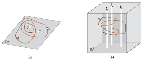
Figure 2: Loops circling a same hinge are equivalent; in both (a) and (b), $\gamma_{\alpha}=\gamma_{\beta}\neq\gamma_{c}$.

The regularization will be discusses in detail in the next section.

III Regge calculus and Discrete Geometry

In this section, we briefly describe discrete geometry as a discretization of a differentiable manifold. The simplest discretization is a simplicial complex, where each discrete element is a simplex. A $p$-simplex is the simplest, flat, $p$-dimensional polytope embedded in an $n$-dimensional space $\mathbb{R}^{n}$, with $n\geq p$. It is constructed from $\left(p+1\right)$ numbers of $\left(p-1\right)$-simplices, such that the lower dimensional simplices are nested into higher dimensional one. The reason for using a simplicial complex as a discretization of a continuous manifold is due to the fact that a simplex is completely determined by their edges key-59 .

The discretization of general relativity had first been studied by Regge, in the second order formulation, this is known as Regge Calculus key-33 ; key-34 . The powerful approach of Regge calculus is in writing the discrete general relativity formulation without the use of coordinate, i.e., using scalar variables such as angle, length, and area, instead of vectorial variables key-33 ; key-34 . It has been shown that discrete gravity will coincide with GR in the classical limit, at the level of the action, when the discrete manifold converges to Riemannian manifold key-33 . However, some aspects of the theory are not entirely complete, for the research in Regge gravity is still continued to grow towards many directions.

III.1 Triangulations: Primal and Dual Lattices.

The works in discrete geometry and Regge calculus mostly use the Delaunay lattice for a discretization, such that the vertex of one polytope is always outside the circumcircles of the others in the lattices key-60 . For this reason, the simplicial complex is sometimes refered as Delaunay triangulation.

A definition of a dual lattice is important for a measurement of the geometric quantities. This, in return, is important if one needs to define the action for the dynamical part of the theory key-55 ; key-57 ; key-61 . Some example of dual lattices commonly used in the literature are circumcentric or barycentric dual lattices, which are defined by connecting their circumcenter and barycenters points key-62 . If the discretization is a Delaunay triangulation, its circumcentric dual is a Voronoi lattice key-62 . Another type of dual lattice, which is important particularly in loop quantum gravity, it the topological / combinatorial, abstract dual lattice. The abstract-dual of a complex could be defined as the circumcentric lattice, but without a fix shape and distance key-63 ; key-64 . In other words, the abstract dual lattice is constructed from graphs, where only the combinatorial aspects of the graph are important. This is similar with the framework adopted in the canonical (loop) quantum gravity key-21 ; key-22 .

In this article, we use the Delaunay triangulation as the primal lattice and an abstract-dual (or combinatorial) lattice as its dual. The reason for this is explained as follows. Let $\mathcal{F}_{\Delta}$ be the primal lattice of a discretization of an $n$-dimensional manifold $\mathcal{F}$, and $\star\mathcal{F}_{\Delta}$ be the circumcentric (or barycentric) dual. Let $\Omega_{\Delta}$ be a discretization of an $\left(n-1\right)$-dimensional hypersurface $\Omega\subset\mathcal{F}$. $\Omega_{\Delta}\subset\mathcal{F}_{\Delta},$ such that the $\left(n-1\right)$-simplices defining $\Omega_{\Delta}$ construct the $n$-simplices of $\mathcal{F}_{\Delta}.$ Moreover, we could define the circumcentric (or barycentric) dual of $\Omega_{\Delta}$, labeled as $\star\Omega_{\Delta}.$ The reason of not using both the circumcentric and barycentric dual, is because it has not been clear if $\star\Omega_{\Delta}\subset\star\mathcal{F}_{\Delta}$, which is important in our construction of the hypersurface slicing. Therefore, it is more convenient to use the combinatorial graph, where the relation $\star\Omega_{\Delta}\subset\star\mathcal{F}_{\Delta}$ could always be defined.

Let us take a specific example of a primal and dual lattice: Suppose $\mathcal{F}_{\Delta}$ is a triangulation of a 3-dimensional manifold $\mathcal{F}.$ $\mathcal{F}_{\Delta}$ is discretized by tetrahedra, which are described using 3-forms. Embedded in $\mathcal{F}_{\Delta}$, one could have lower-dimensional simplices: triangles, segments, and points. With the definition of the abstract-dual lattice, one could define the following terminologies, adopted from the canonical LQG, as described in FIG. 3.

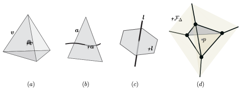
Figure 3: (a) A tetrahedron in a primal lattice $\mathcal{F}_{\Delta}$, labeled by its volume $\boldsymbol{v},$ is dual to the vertex $\star\boldsymbol{v},$ in $\star\mathcal{F}_{\Delta}$. (b) A triangle in $\mathcal{F}_{\Delta}$, labeled by its area $\boldsymbol{a}$ is dual to the edge $\star\boldsymbol{a}$ in $\star\mathcal{F}_{\Delta}.$ (c) A segment $\boldsymbol{l}$ in $\mathcal{F}_{\Delta}$ is dual to the face $\star\boldsymbol{l}$ in $\star\mathcal{F}_{\Delta}.$ (d) A point $p$ in $\mathcal{F}_{\Delta}$ is dual to the 3D-bubble in $\star\mathcal{F}_{\Delta}$.

The introduction of the primal and dual cells will be extremely useful for the rest of this article. In particular, the equivalent class of loops could be defined using a standard loop, which is naturally the boundary of the face, dual to the hinge key-54 . All possible loops circling hinge $\star\hat{\boldsymbol{J}}$ are represented by the standard loop.

III.2 Curvatures

In the framework of Regge calculus, the length of a geometrical object has finite minimal size. This is followed by the finiteness of the size of higher dimensional objects: area, and higher dimensional volumes.

It had been discussed previously that the components of the curvature 2-form are infinitesimal rotations, where the planes of rotation are dual to the infinitesimal hinges. For discrete geometry, the regularization is straightforward: the ’discrete’ curvature 2-form is a finite rotation on a finite hinge. As for finite rotations, it can be represented in two standard ways: the plane-angle (or area-angle key-59 ) and the holonomy representation key-44a .

III.2.1 Plane-angle representation.

In this representation, rotation is describe by a couple $\left(\boldsymbol{J},\delta\phi\right)$, with $\boldsymbol{J}\in\mathfrak{so(n)}$ is an element of Lie algebra as the plane of rotation and one (real) parameter group $\tau$ times the norm of the algebra $\left|\boldsymbol{J}\right|$ for the angle of rotation $\delta\phi$. In the Regge Calculus picture, the intrinsic curvature is represented by the angle of rotation, or the deficit angle, located on the hinge:

$$\delta\phi=2\pi-\sum_{i}\phi_{i}.$$

Non-trivial value of $\delta\phi$ describe the deviation of a space from being flat, see FIG. 4 for a 2-dimensional case.

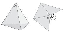
Figure 4: Suppose $\Omega_{\Delta}$ is a 2D surface discretized by three triangles. Point $p$ is the hinge where the deficit angle $\delta\phi$ is located. $\delta\phi$ is the 2D intrinsic curvature of $\Omega_{\Delta}$ at point $p$.

Any components of a test vector $\boldsymbol{V}$ carried around a loop $\gamma$ will be rotated by the deficit angle $\delta\phi$ in the direction of the plane of rotation, which in turns, is perpendicular to the hinge key-54 . The plane-angle representations give a natural definition of curvature in the background independence picture of gravity.

III.2.2 Holonomy Representation, Exponential and Differential Map.

Relation (14), is a map sending the holonomy, which is an element of a rotation group, $\boldsymbol{H}\in SO\left(n\right)$, to the plane-angle representation, commonly refered as the exponential map. As explained earlier, holonomy representation provides a natural way to go from the ’infinitesimal’ continuous to the ’finite’ discrete theory. For a special case where area inside the loop $a$ is chosen to be a square $\boldsymbol{s}_{i}\boldsymbol{s}_{j}$, with $\boldsymbol{s}_{i}=\ell\hat{\boldsymbol{s}}_{i}$ and $\hat{\boldsymbol{s}}_{i}$ is a unit vector, (13) describe a direct ’finite’ version of the curvature 2-form as follows:

$$\boldsymbol{H}_{\gamma}\left(\boldsymbol{A},\gamma_{\mathcal{O},a}\right)=\boldsymbol{1}+\frac{\ell^{2}}{2}\boldsymbol{F}\left(\hat{\boldsymbol{s}}_{i},\hat{\boldsymbol{s}}_{j}\right)+O\left(\ell^{3}\right),$$ (15)

in other words, the curvature 2-form is the holonomy on an infinitesimal loops.

As the inverse of the exponential map, one has the differential map, which sends plane-angle representation to the holonomy representation. This can be obtained from the following procedure: the angle of rotation $\delta\phi$ can be obtained from the trace of the holonomy, which for a special case $\mathcal{G}\sim SO\left(n\right)$, gives:

$$\textrm{tr}\boldsymbol{H}_{\gamma}=n-2\left(1-\cos\delta\phi\right),$$ (16)

with $n$ is the dimension of the rotation matrix, while the plane of rotation $\boldsymbol{J}$ can be obtained from the differential map:

$$\left.\frac{d}{d\delta\phi}\right|_{\delta\phi=0}:\mathcal{G} \rightarrow \mathfrak{g}$$

$$\boldsymbol{H} \mapsto \boldsymbol{J}=\left.\frac{d\boldsymbol{H}}{d\delta\phi}\right|_{\delta\phi=0}.$$

The map from the holonomy to the plane-angle representation is 1-to-1 and onto.

III.2.3 Addition of Two Rotations.

Another important property which is useful is the product of two rotations. In the holonomy representation, the product of two holonomies is simply the matrix multiplication between two holonomies as follows:

$$\boldsymbol{H}_{12}\left(\boldsymbol{A},\gamma_{12}\right)=\boldsymbol{H}_{1}\left(\boldsymbol{A},\gamma_{1}\right)\boldsymbol{H}_{2}\left(\boldsymbol{A},\gamma_{2}\right),$$ (17)

which in general is not commutative: $\boldsymbol{H}_{1}\boldsymbol{H}_{2}\neq\boldsymbol{H}_{2}\boldsymbol{H}_{1}.$ This product defines the piecewise-linear aspect of discrete manifold.

In the plane-angle representation, the product formula is more complicated. The total angle of rotation formula can be obtained by taking trace of (17); this, in particular, depends on the dimension of the space. As an example, for a special case $\mathcal{G}\sim SU\left(2\right)$, the element of the group can be written as follows:

$$\boldsymbol{H}_{i}=\boldsymbol{I}\cos\theta_{i}+\boldsymbol{J}_{i}\sin\theta_{i},$$ (18)

so that it gives the following total angle of rotation formula:

$$\cos\theta_{12}=\cos\theta_{1}\cos\theta_{2}-\cos\bar{\phi}_{12}\sin\theta_{1}\sin\theta_{2},$$ (19)

with $\bar{\phi}_{12}$ is the angle between plane $\boldsymbol{J}_{1}$ and $\boldsymbol{J}_{2}$. The total plane of rotation $\boldsymbol{J}_{12}$ for $\theta_{12}$ can be obtained from the Baker-Campbell-Hausdorff formula. For $\mathcal{G}=SU\left(2\right)$, the total plane formula is the following:

$$\boldsymbol{J}_{12}=\frac{\left(\boldsymbol{I}\cos\theta_{1}+\boldsymbol{J}_{1}\sin\theta_{1}\right)\left(\boldsymbol{I}\cos\theta_{2}+\boldsymbol{J}_{2}\sin\theta_{2}\right)-\boldsymbol{I}_{2\times 2}\cos\theta_{12}}{\sin\theta_{12}}.$$ (20)

III.2.4 Conjugation and Adjoint Representation.

Let $\boldsymbol{g},\boldsymbol{h}\in\mathcal{G}$, then suppose one has the following conjugation induced by $\boldsymbol{g}$ as follows:

$$\boldsymbol{h}^{{}^{\prime}}=\boldsymbol{g}^{-1}\boldsymbol{h}\boldsymbol{g}.$$ (21)

Using the exponential map on $\boldsymbol{h}$ and $\boldsymbol{h}^{\prime}$, one has:

$$\exp\left(\boldsymbol{J}_{h}^{{}^{\prime}}\phi\right)=\boldsymbol{g}^{-1}\exp\left(\boldsymbol{J}_{h}\phi\right)\boldsymbol{g}$$

where $\phi\sim$$\textrm{tr}\boldsymbol{h}=\textrm{tr}\boldsymbol{h}^{\prime}$ is invariant under conjugation. By Taylor expansion up to the first order:

$$\boldsymbol{J}_{h}^{{}^{\prime}}\phi+O\left(\phi^{2}\right)=\boldsymbol{g}^{-1}\boldsymbol{J}_{h}\boldsymbol{g}\phi+\boldsymbol{g}^{-1}O\left(\phi^{2}\right)\boldsymbol{g},$$

for each order $n^{th}$, one has $\boldsymbol{J}_{h}^{{}^{\prime}n}=\boldsymbol{g}^{-1}\boldsymbol{J}_{h}^{n}\boldsymbol{g},$ which is equal to $\boldsymbol{J}_{h}^{{}^{\prime}n}=\left(\boldsymbol{g}^{-1}\boldsymbol{J}_{h}\boldsymbol{g}\right)^{n}.$ Therefore, one obtains:

$$\boldsymbol{J}_{h}^{{}^{\prime}}=\boldsymbol{g}^{-1}\boldsymbol{J}_{h}\boldsymbol{g},$$ (22)

which is the adjoint representation of the Lie group. Conjugation on the group (21) induces a transformation of the Lie algebra by (22). This will be useful when one consider a transformation of planes with different origin.

III.3 Loops, Hinges, and Contractibility

To understand clearly the concept of curvatures in discrete geometry, one needs to include the concept of contractible space. As a simple explanation, a topological space is contractible if it can be continuously shrunk to a point key-65 . Let us consider the following examples: All loops embedded in $\mathbb{R}^{2}$ or $\mathbb{S}^{2}$ are contractible. Some loops living in a torus $\mathbb{T}^{2}$ are non-contractible. Some loops living in $\mathbb{R}^{2}-\left\{0\right\}$ are non-contractible. In higher dimension, all loops living in $\mathbb{R}^{3}-\left\{0\right\}$ are contractible, but some complete closed surface (2-dimensional ’loop’, topologically equivalent to $\mathbb{S}^{2}$) living in $\mathbb{R}^{3}-\left\{0\right\}$ are non-contractible. This can be generalized to any dimension. See FIG. 5.

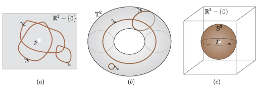
Figure 5: In $\mathbb{R}^{2}-\left\{0\right\}$, with $p$ as the origin (a), and in a 2-dimensional torus $\mathbb{T}^{2}$ (b), $\gamma_{a}$ and $\gamma_{b}$ are non-contractible, $\gamma_{c}$ is contractible. (c) In $\mathbb{R}^{3}-\left\{0\right\}$, a 2-sphere $\mathbb{S}^{2}$ centered at the origin is non-contractible, while any loop $\gamma$ is contractible.

Intuitively, the existence of a ’hole’ contributes to the non-simply connectedness of the manifold. In the context of Regge calculus, the hinge, a $p$-form where the curvature (in the form of deficit angle) is concentrated, acts as a $p$-dimensional ’hole’. To be precise, in 2-dimensional dicrete geometry, the ’hole’ is a point, in 3-dimension, the ’hole’ is an edge, in 4-dimension, is a triangle, in $n$-dimension, the $\left(n-2\right)$ ’hole’, is an $\left(n-2\right)$-simplex. The existence of hinges in discrete manifold defines non-contractible loops. These non-contractible loops are endowed with non-trivial holonomies related to the deficit angles on the hinges, describing the curvature of the discrete manifold. Two different non-contractible loops encircling the same hinges are equivalent through an equivalence class defined earlier in the previous section. Any contractible loop is endowed with trivial holonomy. See FIG. 6.

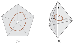
Figure 6: Loop $\gamma$ is non-contractible due to the existence of a hinge, (a) in 2-dimensional triangulation example, and (b) in 3-dimensional triangulation example.

IV 2+1 Regge Calculus

Now we are ready to perform the ADM slicing on a 3-dimensional discrete manifold. The procedure is important, in particular, as a lower dimensional model for the (3+1) ADM slicing of 4-dimensional spacetime, which is the first step to obtain the canonical quantization of gravity key-40 . Works on this field are already developed, for instance, in key-37 ; key-38 ; key-39 ; key-40 ; key-41 ; key-42 ; key-43 ; key-44 ; key-44a . We use the powerful tools of Regge calculus, where the simplices are describe by coordinates-free variables, rather than vectorial elements.

IV.1 The Construction of (2+1) Lattice in First Order Formulation

As a first step, we need to clarify and to gain insight of the geometrical picture of the continuous first order formulation of gravity. Let us use a local coordinate with orthonormal basis $\left(\partial_{x},\partial_{y},\partial_{z}\right)$ to characterize the 3-dimensional base manifold $M$. Let use take point $\mathcal{O}$ as the origin. One could define the planes $dx\wedge dy$, $dy\wedge dz$, $dz\wedge dx$ $\in\Lambda^{2}\left(T_{\mathcal{O}}M\right).$ These are the loop orientation planes, where the three infinitesimal loops $\delta\gamma_{\mu\nu}$ are defined as the (square) boundary of the plane $dx^{\mu}\wedge dx^{\nu},$ See FIG. 7(a).

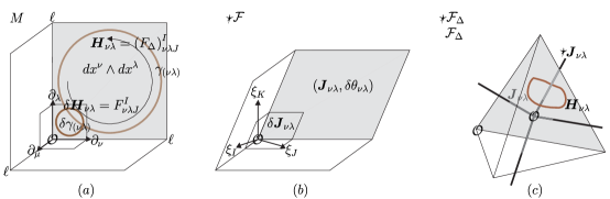
Figure 7: (a) The infinitesimal and finite loop orientation in base space $M$. (b) The infinitesimal and finite plane of rotation in dual fibre $\star\mathcal{F}$. (c) (b) is topologically equivalent with the tetrahedral lattice in (c). Each triangle $\hat{\boldsymbol{J}}_{\mu\nu}$ of the dual lattice is perpendicular to the hinge $\star\hat{\boldsymbol{J}}_{\mu\nu}$.

On these loops, the curvature 2-form components are attached: $F_{xyJ}^{I},$ $F_{yzJ}^{I},$ $F_{zxJ}^{I},$ which describe infinitesimal rotations, namely the rotation bivectors (or plane of rotations). Let use relabel these components as $\delta\hat{\boldsymbol{J}}_{xy}$, $\delta\hat{\boldsymbol{J}}_{yz}$, $\delta\hat{\boldsymbol{J}}_{zx}$ $\in\Lambda^{2}\left(\star\mathcal{F}\sim\mathbb{R}^{3}\right)$. These three rotation bivector planes, in general, are not orthogonal to each other, see FIG. 7(b).

Now, let us clarify the geometrical picture of the first order formulation of Regge calculus. This had been done partially in key-36 . Let us define the finite loop orientation planes $\ell^{2}dx^{\mu}\wedge dx^{\nu}$ $\in\Lambda^{2}\left(T_{\mathcal{O}}M\right),$ with loops $\gamma_{\mu\nu}$ as their boundaries. On these finite loops, the finite curvature 2-form components are attached: $\left(F_{\Delta}\right)_{\mu\nu J}^{I},$ describing finite rotation, which are indeed the holonomy. Relabeling these finite rotation as holonomies $\boldsymbol{H}_{xy}$, $\boldsymbol{H}_{yz}$, $\boldsymbol{H}_{zx}$, it is clear that they satisfy (14), i.e., $\boldsymbol{H}_{\mu\nu}$ are exponential map of $\hat{\boldsymbol{J}}_{\mu\nu}.$ The geometrical interpretation of the finite version is similar with the infinitesimal ones, as compared in FIG. 7(a)-(b).

For each loop defined in $M,$ there exist a corresponding plane of rotation in $\Lambda^{2}\left(\star\mathcal{F}\sim\mathbb{R}^{3}\right)$. The collection of planes of rotation $\hat{\boldsymbol{J}}_{\mu\nu}$ defined an (abstract) dual-lattice $\star\mathcal{F},$ see FIG. 7(c). The corresponding primal lattice of $\star\mathcal{F},$ is (a simplicial complex) $\mathcal{F}$, where dual of the planes of rotations $\hat{\boldsymbol{J}}_{\mu\nu}$ are the hinges $\star\hat{\boldsymbol{J}}_{\mu\nu},$ see FIG. 7(c). For discrete geometry, it is convenient to drop the base manifold picture and focus only on the fibre $\mathcal{F}_{\triangle}$. This includes the ’moving’ of holonomy $\boldsymbol{H}_{\mu\nu}$ (which are located on $M)$ to $\star\mathcal{F}_{\triangle}$, circling hinge $\star\hat{\boldsymbol{J}}_{\mu\nu},$ as in FIG. 7(c). For the next section, we will only focus on the fibre lattice $\mathcal{F}_{\triangle}$ and its dual $\star\mathcal{F}_{\triangle}.$

IV.2 Terminologies of a 4-1 Pachner moves

As already been explained in the previous sections, to describe completely a curvature of a 3-dimensional space, one needs three hinges. On each hinge, which in 3-dimension is a segment, a standard loop is defined as the boundary of the faces in the $\star\mathcal{F}_{\triangle}$, and the holonomy related to the curvature on the hinge is attached on the loop. These three distinct holonomies are the finite version of the three matrices elements of curvature 2-form in 3-dimension. If in the previous section we label the curvature tensor components by the infinitesimal loop orientation planes: $\boldsymbol{F}\left(\partial_{\mu},\partial_{\nu}\right),$ $\boldsymbol{F}\left(\partial_{\nu},\partial_{\lambda}\right),$ $\boldsymbol{F}\left(\partial_{\lambda},\partial_{\nu}\right),$ now we use the hinges to label the finite versions, say $\boldsymbol{H}_{i},$ with $\boldsymbol{l}_{i}$ describing the finite hinge $i$. Therefore, the simplest dicretization in three dimension which yield a complete curvature is the discretization by the 4-1 Pachner move, see FIG. 8(a).

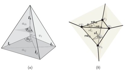
Figure 8: 4-1 Pachner move (a) in primal lattice, and (b) in abstract-dual lattice.

The holonomies in 3-dimension are elements of rotation group $SO\left(3\right),$ but for our work, we use its complex counterpart, which is also its double-cover, the group $SU\left(2\right)$. The reason for this, is because the formulations can be written more compactly using the $SU\left(2\right)$ group.

The 4-1 Pachner move is the boundary of a 4-simplex, where four tetrahedra meet each other on their triangles. A 4-simplex, and similarly, its boundary, can completely and uniquely be described by the length of its ten segments key-59 ; key-66 . These variables are coordinate free, i.e., they are not vectorial. Another different set of a complete coordinate-free variables containing equivalent informations of the move are the length of four internal segments and six internal 2D angles key-66 ; this will be our starting point. We define the terminologies of 4-1 Pachner moves as follows. Each one of the four internal segments of the move are 3-dimensional hinge. We label them with $\boldsymbol{l}_{i}$, with $i=1,..,4$. The six remaining variables are described by the six angles $\phi_{ij}$ between segment $\boldsymbol{l}_{i}$ and $\boldsymbol{l}_{j}$, located at the center point, see FIG. 8(a). These are 2-dimensional angles. Furthermore, a triangle $\boldsymbol{a}_{ij}$ is the plane between segment $\boldsymbol{l}_{i}$ and $\boldsymbol{l}_{j}$. On each segment $\boldsymbol{l}_{k}$, three 3-dimensional (dihedral) angles $\theta_{ij,k}$ are located, which are the angles between plane $\boldsymbol{a}_{ik}$ and $\boldsymbol{a}_{jk}$. The last geometric figures are tetrahedra $\boldsymbol{v}_{i},$ constructed from the three segments $\boldsymbol{l}_{i}$, $\boldsymbol{l}_{j}$, and $\boldsymbol{l}_{k}$. See FIG. 8(a). The abstract dual lattice is described in FIG. 8(b). Vertices $\star\boldsymbol{v}_{i}$ are dual to primal tetrahedra, edges $\star\boldsymbol{a}_{ij}$ are dual to primal triangle, and faces $\star\boldsymbol{l}_{i}$ are dual to primal segments.

The measure of the geometric quantities, such as length, area, and volume, for the moment, is not included in our work, since we are only interested in the cuvatures, which only needs the information of the angles. But for further works including the dynamics of the theory, it is possible to provide our construction with a geometric measure, i.e, attaching ’norms’ on the lattices by a well-defined procedure; in particular, the hybrid cells introduced in key-46 ; key-49 ; key-54 .

IV.3 Curvatures, Closure Constraint, and Bianchi Identity

A 3-dimensional holonomy of connection $\boldsymbol{A}\in\mathfrak{su\left(2\right)}$ along curve $\gamma$ with origin $\mathcal{O}$ is written as:

$$\boldsymbol{H}_{\gamma}=\boldsymbol{H}_{\gamma}\left(\boldsymbol{A},\gamma_{\mathcal{O}}\right).$$

We will simplify the notation as long as the meaning it describe is clear and non-ambiguous.

As a first step, let us define the 3-dimensional holonomy on edge $\star\boldsymbol{a}_{ij}$ between vertex $\star\boldsymbol{v}_{i}$ and $\star\boldsymbol{v}_{j}$ as $\boldsymbol{H}_{ij}$, see FIG. 9(a).

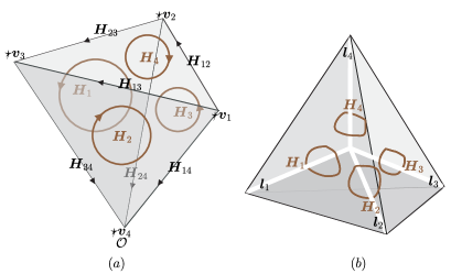
Figure 9: The generalized closure constraint in (a) the dual lattice, topologically equivalent to a tetrahedron, and in (b) the primal lattice.

Notice that $\boldsymbol{H}_{ij}$ is attached on an open curve with the origin $\star\boldsymbol{v}_{i}$ towards $\star\boldsymbol{v}_{j}$, so that it does not satisfies (15). The inverse is:

$$\boldsymbol{H}_{ji}=\boldsymbol{H}_{ij}^{-1},$$

with origin $\star\boldsymbol{v}_{j}$ towards $\star\boldsymbol{v}_{i}$. The next step is to define the 3-dimensional holonomy on a closed loop, where the loop is the boundary of the faces $\star\boldsymbol{l}_{i}$: a standard loop, as follows:

$$\boldsymbol{H}_{i}\left(\boldsymbol{A},\gamma_{i,\star\boldsymbol{v}_{j}}\right)=\boldsymbol{H}_{jk}\boldsymbol{H}_{kl}\boldsymbol{H}_{lj}.$$ (23)

$\boldsymbol{H}_{i}$ is the holonomy around the loop $\gamma_{i}$ circling hinge $\boldsymbol{l}_{i}$ with origin $\star\boldsymbol{v}_{j}$.

IV.3.1 Generalized Closure Constraint.

As already studied in key-67 , a curved tetrahedron satisfies the generalized closure constraint governed by its holonomies. We will use the result in this subsection. The 4-1 Pachner move contains four internal hinges and therefore four planes of rotation dual to the hinges, but only three of them are independent, such that the following ’closure constraint’ is satisfied:

$$\boldsymbol{H}_{1}\boldsymbol{H}_{2}\boldsymbol{H}_{3}\overline{\boldsymbol{H}}_{4}=\boldsymbol{1},$$ (24)

This relation is taken with the vertex $\star\boldsymbol{v}_{4}$ as the origin. More precisely:

$$\boldsymbol{H}_{1}=\boldsymbol{H}_{1}\left(\boldsymbol{A},\gamma_{1,\star\boldsymbol{v}_{4}}\right) = \boldsymbol{H}_{42}\boldsymbol{H}_{23}\boldsymbol{H}_{34},$$

$$\boldsymbol{H}_{2}=\boldsymbol{H}_{2}\left(\boldsymbol{A},\gamma_{2,\star\boldsymbol{v}_{4}}\right) = \boldsymbol{H}_{43}\boldsymbol{H}_{31}\boldsymbol{H}_{14},$$ (25)

$$\boldsymbol{H}_{3}=\boldsymbol{H}_{3}\left(\boldsymbol{A},\gamma_{3,\star\boldsymbol{v}_{4}}\right) = \boldsymbol{H}_{41}\boldsymbol{H}_{12}\boldsymbol{H}_{24},$$

$$\overline{\boldsymbol{H}}_{4}=\overline{\boldsymbol{H}}_{4}\left(\boldsymbol{A},\gamma_{4,\star\boldsymbol{v}_{4}}\right) = \boldsymbol{H}_{42}\underset{\boldsymbol{H}_{4}\left(\boldsymbol{A},\gamma_{4,\star\boldsymbol{v}_{2}}\right)}{\underbrace{\boldsymbol{H}_{21}\boldsymbol{H}_{13}\boldsymbol{H}_{32}}}\boldsymbol{H}_{24}=\boldsymbol{H}_{123}^{-1}.$$

See FIG. 9(a). There is a gauge freedom in choosing path $\overline{\boldsymbol{H}}_{4}$, which in this case, is gauge-fixed by taking the path through $\boldsymbol{H}_{42}$ from the origin. Other paths are possible, see the explanation in key-67 . Any tetrahedral lattice as in FIG. 9(a) will satisfy (24). In the primal lattice point of view, the closure constraint guarantees that a sets of four tetrahedra, connected to each other on their internal faces, construct a closed, (in general) curved tetrahedron. This will be explored in more detail in Subsection V A.

IV.3.2 3D Discrete Intrinsic Curvature.

As explained earlier, one can choose three combinations of distinct holonomies $\boldsymbol{H}_{i},\boldsymbol{H}_{j},\boldsymbol{H}_{k}$ from the four in (25) as the finite version of curvature 2-form. They contain the information of the 3-dimensional discrete curvature as well as the curvature 2-form $\,{}^{3}\boldsymbol{F}_{IJ}$ contains for the continuous space. We label the components of discrete intrinsic 3D curvature as the following three tuples of holonomies:

$$\left(\,{}^{3}\boldsymbol{F}_{\triangle}\right)_{\mu\nu}=\boldsymbol{H}_{\mu\nu}\left(\boldsymbol{A},\gamma_{\mu\nu,\mathcal{O}}\right)=\left(\boldsymbol{H}_{1}\left(\boldsymbol{A},\gamma_{1,\mathcal{O}}\right),\boldsymbol{H}_{2}\left(\boldsymbol{A},\gamma_{2,\mathcal{O}}\right),\boldsymbol{H}_{3}\left(\boldsymbol{A},\gamma_{3,\mathcal{O}}\right)\right).$$ (26)

Furthermore, we will drop the indices $\mu,\nu$ and write the components (26) as $\,{}^{3}\boldsymbol{F}_{\triangle}$ for simplicity. The corresponding plane-angle representation can be obtained from the trace and differential map of (26):

$$\,{}^{3}\boldsymbol{F}_{\triangle}=\left\{\left(\delta\theta_{1},\left.\hat{\boldsymbol{J}}_{1}\right|_{\mathcal{O}}\right),\left(\delta\theta_{2},\left.\hat{\boldsymbol{J}}_{2}\right|_{\mathcal{O}}\right),\left(\delta\theta_{3},\left.\hat{\boldsymbol{J}}_{3}\right|_{\mathcal{O}}\right)\right\},$$

with the deficit angle on hinge $\boldsymbol{l}_{i}$ satisying (16) and:

$$\delta\theta_{i}=2\pi-\left(\sum_{j,k}\theta_{jk,i}\right),\qquad j,k\neq i,\,j<k.$$ (27)

and the rotation bivector with origin $\mathcal{O}$ satisfying:

$$\left.\hat{\boldsymbol{J}}_{i}\right|_{\mathcal{O}}=\left.\frac{d\boldsymbol{H}_{i}}{d\delta\theta_{i}}\right|_{\delta\theta_{i}=0}.$$ (28)

See FIG. 10.

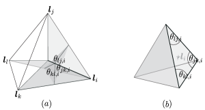
Figure 10: The 3-dimensional discrete intrinsic curvature on hinge in (a) primal lattice, and (b) dual lattice.

IV.3.3 Bianchi Identity.

Before arriving at the discrete version of Bianchi identity, we need to proof an important relation. As explained earlier, any tetrahedral lattice as in FIG. 9(a) always satisfy the generalized closure constraint (24). By a straightforward calculation, (24) can be written as:

$$\boldsymbol{H}_{1}\boldsymbol{H}_{2}\boldsymbol{H}_{3}\overline{\boldsymbol{H}}_{4}=\underset{\boldsymbol{h}_{1}}{\underbrace{\boldsymbol{H}_{42}\boldsymbol{H}_{23}}}\underset{\boldsymbol{h}_{2}}{\underbrace{\boldsymbol{H}_{31}\boldsymbol{H}_{14}}}\underset{\boldsymbol{h}_{3}}{\underbrace{\boldsymbol{H}_{41}\boldsymbol{H}_{12}}}\underset{\boldsymbol{h}_{4}}{\underbrace{\boldsymbol{H}_{21}\boldsymbol{H}_{13}}}\underset{\boldsymbol{h}_{1}^{-1}}{\underbrace{\boldsymbol{H}_{32}\boldsymbol{H}_{24}}.}$$

This immediately gives:

$$\boldsymbol{h}_{1}\boldsymbol{h}_{2}\boldsymbol{h}_{3}\boldsymbol{h}_{4}\boldsymbol{h}_{1}^{-1}=\boldsymbol{1},$$

where the two adjacents holonomies $\boldsymbol{H}_{jk}$ and $\boldsymbol{H}_{kl}$ are collected together as $\boldsymbol{h}_{i}$. In general, for every point $\mathcal{O}$ in the lattice as the origin, the following relation, which we called as ’trivalent condition’, is valid:

$$\boldsymbol{h}_{i}\boldsymbol{h}_{j}\boldsymbol{h}_{k}=\boldsymbol{1},\quad i=1,..4,\>i\neq j\neq k.$$ (29)

Relation (29) could be illustrated by the combinatorics graph in FIG. 11(a).

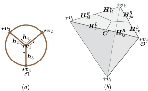
Figure 11: (a) An abstract tetrahedral lattice can be illustrated as above. Holonomies on a trivalent vertex satisfies relation (29), where in this case, is $\boldsymbol{h}_{2}\boldsymbol{h}_{3}\boldsymbol{h}_{4}=\boldsymbol{1}$. (b) Moving the origin from $\mathcal{O}$ to $\mathcal{O}$’.

Holonomies of any trivalent vertex satisfy relation (29). This relation will be important for the derivation of the Bianchi identity in the following paragraph.

Let us split the holonomy $\boldsymbol{H}_{ij}$ as follows:

$$\boldsymbol{H}_{ij}=\boldsymbol{H}_{ij}^{\left(L\right)}\boldsymbol{H}_{ij}^{\left(R\right)},$$ (30)

so that (23) can be rewritten as:

$$\boldsymbol{H}_{i}=\boldsymbol{H}_{jk}^{\left(L\right)}\boldsymbol{H}_{jk}^{\left(R\right)}\boldsymbol{H}_{kl}^{\left(L\right)}\boldsymbol{H}_{kl}^{\left(R\right)}\boldsymbol{H}_{lj}^{\left(L\right)}\boldsymbol{H}_{lj}^{\left(R\right)}.$$

Noted that these holonomies are originated at $\mathcal{O}=\star\boldsymbol{v}_{j}$. Now we move the origin to point $\mathcal{O}^{\prime}$, which is a point on the edge between $\star\boldsymbol{v}_{j}$ and $\star\boldsymbol{v}_{l}$, see FIG. 11(b). $\boldsymbol{H}_{i}$ is transformed into:

$$\boldsymbol{H}_{i}^{{}^{\prime}}\left(\boldsymbol{A},\gamma_{i,\mathcal{O}^{\prime}}\right)=\boldsymbol{H}_{lj}^{\left(R\right)}\boldsymbol{H}_{i}\left(\boldsymbol{A},\gamma_{i,\mathcal{O}}\right)\boldsymbol{H}_{lj}^{\left(R\right)-1}.$$ (31)

Therefore, from point $\mathcal{O}^{\prime}$, the holonomy circling hinge $\boldsymbol{l}_{i}$ is:

$$\boldsymbol{H}_{i}^{{}^{\prime}}=\boldsymbol{H}_{i}^{{}^{\prime}}\left(\boldsymbol{A},\gamma_{i,\mathcal{O}^{\prime}}\right)=\underset{\boldsymbol{h}_{kl,i}}{\underbrace{\boldsymbol{H}_{lj}^{\left(R\right)}\boldsymbol{H}_{jk}^{\left(L\right)}}}\underset{\boldsymbol{h}_{lj,i}}{\underbrace{\boldsymbol{H}_{jk}^{\left(R\right)}\boldsymbol{H}_{kl}^{\left(L\right)}}}\underset{\boldsymbol{h}_{jk,i}}{\underbrace{\boldsymbol{H}_{kl}^{\left(R\right)}\boldsymbol{H}_{lj}^{\left(L\right)}},}$$ (32)

splitted into three holonomies $\boldsymbol{h}_{jk,i}$ on open curves, see FIG. 12(a).

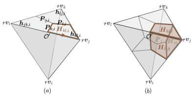
Figure 12: (a). Spliting holonomy into three holonomy on loops. (b) A tetrahedral lattice on a vertex, satisfying the closure and trivalent condition.

The decomposition in (30) is chosen such that $\boldsymbol{h}_{kl,i}$, $\boldsymbol{h}_{jl,i}$, and $\boldsymbol{h}_{jk,i}$, using the trace (16) and differential map (28), satisfy:

$$\boldsymbol{h}_{kl,i} = \exp\left(\boldsymbol{H}_{lj}^{\left(R\right)}\hat{\boldsymbol{J}}_{i}\boldsymbol{H}_{lj}^{\left(R\right)-1}\theta_{kl,i}\right),$$

$$\boldsymbol{h}_{lj,i} = \exp\left(\boldsymbol{H}_{lj}^{\left(R\right)}\hat{\boldsymbol{J}}_{i}\boldsymbol{H}_{lj}^{\left(R\right)-1}\theta_{lj,i}\right),$$ (33)

$$\boldsymbol{h}_{jk,i} = \exp\left(\boldsymbol{H}_{lj}^{\left(R\right)}\hat{\boldsymbol{J}}_{i}\boldsymbol{H}_{lj}^{\left(R\right)-1}\theta_{jk,i}\right).$$

The origin of the rotation bivector plane $\hat{\boldsymbol{J}}_{i}$ is moved from $\mathcal{O}$ to $\mathcal{O}^{\prime}$ using the adjoint representation induced by (31).

The next step is to split $\boldsymbol{H}_{i}^{{}^{\prime}}$ into three holonomies on a loop, with origin $\mathcal{O}^{\prime}$, as follows:

$$\boldsymbol{H}_{i}^{{}^{\prime}}=\boldsymbol{H}_{kl,i}\boldsymbol{H}_{lj,i}\boldsymbol{H}_{jk,i},$$

such that:

$$\boldsymbol{H}_{kl,i} = \boldsymbol{h}_{kl,i}\boldsymbol{P}_{l,i}\boldsymbol{P}_{k,i},$$

$$\boldsymbol{H}_{lj,i} = \boldsymbol{P}_{k,i}^{-1}\boldsymbol{P}_{l,i}^{-1}\boldsymbol{h}_{lj,i}\boldsymbol{P}_{j,i}\boldsymbol{P}_{k,i},$$

$$\boldsymbol{H}_{jk,i} = \boldsymbol{P}_{k,i}^{-1}\boldsymbol{P}_{j,i}^{-1}\boldsymbol{h}_{jk,i},$$

see FIG. 12(a). $\boldsymbol{P}_{k,i}$ are the gauge freedom which can be fixed arbitrarily. Notice that on each vertex $\star\boldsymbol{v}$, there exist a tetrahedral lattice defined by three holonomies on different faces, see FIG. 12(b). The existence of the tetrahedral lattice on each vertex is guaranteed as long as the decomposition (30) satisfies (33). The tetrahedral lattice in vertex $\star\boldsymbol{v}_{j}$, needs to satisfy the closure condition:

$$\boldsymbol{H}_{kl,i}\overline{\boldsymbol{H}}_{ik,l}\boldsymbol{P}_{j}\boldsymbol{H}_{li,k}=1,$$

with:

$$\overline{\boldsymbol{H}}_{ik,l} = \boldsymbol{P}_{k,i}^{-1}\boldsymbol{P}_{l,i}^{-1}\underset{\boldsymbol{h}_{ik,l}\boldsymbol{P}_{k,l}\boldsymbol{P}_{i,l}}{\underbrace{\boldsymbol{H}_{ik,l}}}\boldsymbol{P}_{l,i}\boldsymbol{P}_{k,i},$$

$$\boldsymbol{P}_{j} = \boldsymbol{P}_{k,i}^{-1}\boldsymbol{P}_{l,i}^{-1}\boldsymbol{P}_{i,l}^{-1}\boldsymbol{P}_{k,l}^{-1}\boldsymbol{P}_{l,k}\boldsymbol{P}_{i,k},$$

$$\boldsymbol{H}_{li,k} = \boldsymbol{P}_{l,k}^{-1}\boldsymbol{P}_{i,k}^{-1}\boldsymbol{h}_{li,k}.$$

Since each tetrahedron on the 4-1 Pachner move is a flat 3-simplex, we have:

$$\boldsymbol{P}_{j}=1,$$ (34)

this will be clear in Subsection V A. Moreover, the holonomies meeting on vertex $\star\boldsymbol{v}_{j}$ also needs to satisfies the trivalent condition:

$$\boldsymbol{h}_{kl,i}\boldsymbol{h}_{ik,l}\boldsymbol{h}_{li,k}=\boldsymbol{h}_{kl,i}\left(\boldsymbol{A},\gamma_{i,\mathcal{O}^{{}^{\prime}}}\right)\boldsymbol{h}_{ik,l}\left(\boldsymbol{A},\gamma_{l,\mathcal{O}^{{}^{\prime}}}\right)\boldsymbol{h}_{li,k}\left(\boldsymbol{A},\gamma_{k,\mathcal{O}^{{}^{\prime}}}\right)=1,$$ (35)

which is valid for every point on the lattice. We will show in Subsection V A that (35) is indeed the discrete version of Bianchi identity. This is consistent with a more general version of discrete Bianchi identity defined by the product of $n$ holonomies in key-51 . The Bianchi identity is satisfied universally in any dimension, and in Subsection V A, we will show that in the discrete picture, it is related to the spherical law of cosine and the dihedral angle relation on a simplex.

IV.3.4 2D Intrinsic Curvature.

Inside a 4-1 Pachner move, there exists four natural slicings of the 2-dimensional submanifold, see FIG. 13(a). These 2-dimensional surfaces consist three triangles.

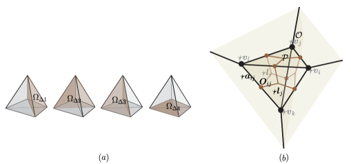
Figure 13: (a). 2-dimensional possible slicings of the 4-1 Pachner moves. (b). The holonomy on each loops of the possible 2-dimensional slices.

The 2-dimensional intrinsic curvature on each of these possible surfaces contains a single rotation matrix and a plane, and therefore, contains a single loop. To label the holonomy, we use similar terminologies with the 3D version, but in one dimension lower: primal triangles are dual to vertices, primal segments are dual to edges, both these edges and vertices are called, respectively, as nodes and links, to distinguish them from the edges and links of the 3D dual lattice.

A 2-dimensional holonomy of connection $\boldsymbol{a}\in\mathfrak{so\left(2\right)}$ along curve $\lambda$ with origin $\mathcal{P}$ is written as:

$$\boldsymbol{O}_{\lambda}=\boldsymbol{O}_{\lambda}\left(\boldsymbol{a},\lambda_{\mathcal{P}}\right).$$

Let us define the 2-dimensional holonomy on a link crossing edge $\star\boldsymbol{a}_{ij}$ (embedded on the half of face $\star\boldsymbol{l}_{i}$ and $\star\boldsymbol{l}_{j}$, in the direction from $\star\boldsymbol{l}_{i}$ to $\star\boldsymbol{l}_{j}$) as $\boldsymbol{O}_{ij}\in\rho_{3}\left(SO(2)\right),$ an element of representation of $SO\left(2\right)$ in three dimension, see FIG. 13(b). The holonomy around a loop, circling the 2D hinge which is the center point $p$, is defined as:

$$\boldsymbol{O}_{i}=\boldsymbol{O}_{jk}\boldsymbol{O}_{kl}\boldsymbol{O}_{lj}.$$

Each $\boldsymbol{O}_{i}$ represents loop on different slice $\Omega_{i}.$ The four loops are connected to each other, and similar with (24), they also satisfy the closure constraint, where $\star\boldsymbol{l}_{4}$ is chosen to be the origin $\mathcal{P}$:

$$\boldsymbol{O}_{1}\boldsymbol{O}_{2}\boldsymbol{O}_{3}\overline{\boldsymbol{O}}_{4}=1,$$ (36)

with:

$$\boldsymbol{O}_{1}=\boldsymbol{O}_{1}\left(\boldsymbol{a},\lambda_{1,\star\boldsymbol{l}_{4}}\right) = \boldsymbol{O}_{42}\boldsymbol{O}_{23}\boldsymbol{O}_{34},$$

$$\boldsymbol{O}_{2}=\boldsymbol{O}_{2}\left(\boldsymbol{a},\lambda_{2,\star\boldsymbol{l}_{4}}\right) = \boldsymbol{O}_{43}\boldsymbol{O}_{31}\boldsymbol{O}_{14},$$

$$\boldsymbol{O}_{3}=\boldsymbol{O}_{3}\left(\boldsymbol{a},\lambda_{3,\star\boldsymbol{l}_{4}}\right) = \boldsymbol{O}_{41}\boldsymbol{O}_{12}\boldsymbol{O}_{24},$$ (37)

$$\overline{\boldsymbol{O}}_{4}=\overline{\boldsymbol{O}}_{4}\left(\boldsymbol{a},\lambda_{4,\star\boldsymbol{l}_{4}}\right) = \boldsymbol{O}_{42}\underset{\boldsymbol{O}_{4}\left(\boldsymbol{a},\lambda_{4,\star\boldsymbol{l}_{2}}\right)}{\underbrace{\boldsymbol{O}_{21}\boldsymbol{O}_{13}\boldsymbol{O}_{32}}}\boldsymbol{O}_{24}=\boldsymbol{O}_{123}^{-1}.$$

See FIG. 13(b).

Let us choose a specific slicing, orthogonal to the hinge $\boldsymbol{l}_{4}$, which is labeled as $\Omega_{4}$. The 2-dimensional intrinsic curvature of $\Omega_{4}$ has a single components, written as follows:

$$\,{}^{2}\boldsymbol{F}_{\triangle}=\overline{\boldsymbol{O}}_{4}=\overline{\boldsymbol{O}}_{4}\left(\boldsymbol{a},\lambda_{4,\mathcal{P}}\right).$$ (38)

The corresponding plane-angle representation is:

$$\,{}^{2}\boldsymbol{F}_{\Delta}=\left(\delta\phi_{4},\left.\boldsymbol{j}_{4}\right|_{\mathcal{P}}\right)=\left(\delta\phi_{4},\boldsymbol{O}_{42}\left.\frac{d\boldsymbol{O}_{4}}{d\delta\phi_{4}}\right|_{\delta\phi_{4}=0}\boldsymbol{O}_{24}\right),$$ (39)

with the deficit angle on hinge $p$ satisying (16) and:

$$\delta\phi_{4}=2\pi-\left(\sum_{j,k}\phi_{jk}\right),\qquad j,k\neq 4,\,j<k.$$

and the rotation bivector with origin $\mathcal{P}$ as:

$$\left.\boldsymbol{j}_{4}\right|_{\mathcal{P}}=\left.\frac{d\overline{\boldsymbol{O}}_{4}}{d\delta\phi_{4}}\right|_{\delta\phi_{4}=0}.$$

As for the trivalent condition, we split holonomy $\boldsymbol{O}_{ij}$ in a similar way with the 3D holonomy as follows:

$$\boldsymbol{O}_{ij}=\boldsymbol{O}_{ij}^{\left(L\right)}\boldsymbol{O}_{ij}^{\left(R\right)},$$

so that (36) can be rewritten as:

$$\boldsymbol{O}_{i}=\boldsymbol{O}_{jk}^{\left(L\right)}\boldsymbol{O}_{jk}^{\left(R\right)}\boldsymbol{O}_{kl}^{\left(L\right)}\boldsymbol{O}_{kl}^{\left(R\right)}\boldsymbol{O}_{lj}^{\left(L\right)}\boldsymbol{O}_{lj}^{\left(R\right)}.$$

The next step is to move the origin from point $\mathcal{P}$ to point $\mathcal{O}^{\prime}$, which is, as explained earlier, a point between $\star\boldsymbol{v}_{j}$ and $\star\boldsymbol{v}_{l}$, see FIG. 14(a). $\boldsymbol{O}_{i}$ is transformed into:

$$\boldsymbol{O}_{i}^{{}^{\prime}}=\boldsymbol{O}_{lj}^{\left(R\right)}\boldsymbol{O}_{i}\boldsymbol{O}_{lj}^{\left(R\right)-1}$$

Therefore, in a similar way with the 3D holonomy, the holonomy circling hinge $p$ according to $\mathcal{O}^{\prime}$ is:

$$\boldsymbol{O}_{i}^{{}^{\prime}}=\underset{\boldsymbol{o}_{kl,i}}{\underbrace{\boldsymbol{O}_{lj}^{\left(R\right)}\boldsymbol{O}_{jk}^{\left(L\right)}}}\underset{\boldsymbol{o}_{jl,i}}{\underbrace{\boldsymbol{O}_{jk}^{\left(R\right)}\boldsymbol{O}_{kl}^{\left(L\right)}}}\underset{\boldsymbol{o}_{jk,i}}{\underbrace{\boldsymbol{O}_{kl}^{\left(R\right)}\boldsymbol{O}_{lj}^{\left(L\right)}},}$$ (40)

splitted into three holonomies $\boldsymbol{o}_{jk,i}$ on open curves, see FIG. 14(b).

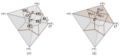
Figure 14: (a). Transformation from $\mathcal{O}$ to $\mathcal{O}^{\prime}$ to $\mathcal{P}$ . (b) Trivalent condition for 2D holonomies.

As a representation of $SU\left(2\right)$ in 3-dimension, the 2D holonomies satisfy the trivalent condition:

$$\boldsymbol{o}_{kl,i}\boldsymbol{o}_{ik,l}\boldsymbol{o}_{li,k}=\boldsymbol{o}_{kl,i}\left(\boldsymbol{a},\gamma_{i,\mathcal{O}^{{}^{\prime}}}\right)\boldsymbol{o}_{ik,l}\left(\boldsymbol{a},\gamma_{l,\mathcal{O}^{{}^{\prime}}}\right)\boldsymbol{o}_{li,k}\left(\boldsymbol{a},\gamma_{k,\mathcal{O}^{{}^{\prime}}}\right)=1,$$ (41)

see FIG. 14(b).

IV.3.5 Extrinsic Curvature.

The definition of extrinsic curvature in discrete geometry is not entirely clear key-29 ; key-44a . Attempts had been done to give it a well-defined definition, in particular, key-48 , and more recently, key-49 ; key-50 . Nevertheless, we choose a different approach for the definition of extrinsic curvature as follows.

The extrinsic curvature (9) of a given slice $\Omega$, in a general gauge condition, is defined as follows:

$$\boldsymbol{K}\left(\boldsymbol{s},\boldsymbol{V}\right)=g\left(D_{\boldsymbol{s}}\tilde{\boldsymbol{n}},\boldsymbol{V}\right),$$ (42)

with $\boldsymbol{s}\in T_{p}M$, $\tilde{\boldsymbol{n}},\boldsymbol{V}\in E_{p}$. $\tilde{\boldsymbol{n}}$, which is a section of a bundle, is a vector normal to the fibre hypersurface $\Omega\subset\mathcal{F}$, moreover, $\boldsymbol{K}\left(\boldsymbol{s},\boldsymbol{V}\right)$ can be geometrically interpreted as the change of normal $\tilde{\boldsymbol{n}}$ in the direction of $\boldsymbol{s}$. One could construct the Lie derivative of the extrinsic curvature, which is an element of $\mathfrak{so\left(n\right)}$ by Theorem I:

$$\boldsymbol{k} = \left[\boldsymbol{K},\boldsymbol{K}\right]=\left(K_{\mu}^{I}K_{\nu}^{J}-K_{\nu}^{I}K_{\mu}^{J}\right)\>\xi_{I}\wedge\xi_{J}\otimes dx^{\mu}\wedge dx^{\nu},$$

$$K_{\mu}^{I} = \boldsymbol{K}\left(\partial_{\mu},\xi^{I}\right)=g\left(D_{\mu}\tilde{\boldsymbol{n}},\xi^{I}\right).$$

$\boldsymbol{k}$ is an infinitesimal rotation on the boundary of plane $a=\ell^{2}dx^{\mu}\wedge dx^{\nu}$. Therefore, we could define the holonomy of extrinsic curvature $\boldsymbol{k}$ along the loop, by (12) as follows:

$$\mathcal{\boldsymbol{K}}=\hat{P}\exp\int_{a}\boldsymbol{k},$$ (43)

but it is not clear if $\boldsymbol{k}$ comes from a connection, i.e., if $\boldsymbol{k}$ is a differential of a 1-form $\boldsymbol{a}_{k}$ such that $d_{D}\boldsymbol{a}_{k}=\boldsymbol{k}$. (43) can be expanded into:

$$\mathcal{\boldsymbol{K}}\left(\gamma_{\mathcal{O}}\right)=\boldsymbol{1}+\ell^{2}\boldsymbol{k}+O\left(\ell^{3}\right).$$ (44)

We could obtain a discrete version of $\mathcal{\boldsymbol{K}}$ as follows. For the first step, we will obtain the corresponding angle of rotation. Given a prefered slicing $\Omega_{4}$, relation (27), which describe the 3-dimensional deficit angle $\delta\theta_{i}$ on each internal segment of the move, can be rewritten as follows:

$$\delta\theta_{i}=2\pi-\left(\underset{\theta_{i}}{\underbrace{\theta_{jk,i}}}+\underset{\bar{\theta}_{i}}{\underbrace{\theta_{j4,i}+\theta_{k4,i}}}\right),\qquad i,j,k=1,2,3,\>i\neq j\neq k,$$ (45)

where $\theta_{i}$, with respect to tetrahedron $\boldsymbol{v}_{4}$, is the internal dihedral angle, and $\bar{\theta}_{i}$ is the external dihedral angle coming from the dihedral angles of other tetrahedra key-44a , see FIG. 15.

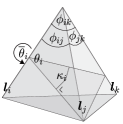
Figure 15: Internal and external dihedral angles. From the dihedral angle relation, we could obtain the internal dihedral angle $\theta_{i}$ on a segment. $\bar{\theta}_{i}$ is the external dihedral angle, while $\kappa_{i}$ is the angle between normals of the two triangles.

Following the definition in our previous work key-44a , let us introduce the quantity:

$$\kappa_{i}=\bar{\theta}_{i}-\pi.$$ (46)

For the case where $\mathcal{F}_{\Delta}$ is flat, $\delta\theta_{i}=0$. This causes $\theta_{i}+\bar{\theta}_{i}=2\pi,$ and using definition (46), we obtain:

$$\theta_{i}+\kappa_{i}=\pi.$$

In this flat case, it is clear that $\kappa_{i}$ is the angle between the normals of two triangles, see FIG. 15.

We can write $\kappa_{i}$ as:

$$\kappa_{i}=\pi-\left(\delta\theta_{i}+\theta_{i}\right),$$ (47)

with $\theta_{i}$ is the internal dihedral angle. Therefore, we define $\kappa_{i}$ as the 2-dimensional deficit angle of the extrinsic curvature, because it is in accordance with the definition of extrinsic curvature (42), where $\boldsymbol{\mathcal{K}}$ is defined as the covariant derivative of the normal $\tilde{\boldsymbol{n}}$ to the hypersurface $\Omega$. It will inherit the curvature of the 3-dimensional manifold.

The discrete holonomy of extrinsic curvature on hinge $\boldsymbol{l}_{i}$ can be written as:

$$\mathcal{\boldsymbol{K}}_{\Delta i}\left(\gamma_{\mathcal{O}}\right)=\exp\left(\left.\boldsymbol{J}_{i}\right|_{\mathcal{O}}\kappa_{i}\right),$$ (48)

with $\left.\boldsymbol{J}_{i}\right|_{\mathcal{O}}$ satisfying (28) and $\kappa_{i}$ satisfying (47).

Another way to obtain the discrete extrinsic curvature exist, which yields the following relation:

$$\boldsymbol{\mathcal{K}}_{ij,k}\left(\gamma_{\mathcal{O}^{\prime}}\right)=\boldsymbol{h}_{kj,i}^{{}^{\prime}}\boldsymbol{O}_{ij}^{{}^{\prime}-1}\boldsymbol{h}_{ik,j}.$$ (49)

(49) is a consequence of the Gauss-Codazzi equation. In the next sections, we will show that (48) and (49) yields similar deficit angles, but located on different hinges; and both of these definitions will coincide in the continuum limit.

IV.4 The Discrete Gauss-Codazzi Equation

IV.4.1 Geometrical Settings

The continuous Gauss-Codazzi equation is defined on each point on an arbitrary manifold $\mathcal{F}$. By introducing a regulator which ’blows’ a points into $n$-dimensional ’bubbles’ (that is, an $n$-dimensional simplex in the dual lattice $\star\mathcal{F}_{\triangle}$, see FIG. 3(d)), and using the fact that bubbles is constructed from several loops meeting together, we could define the discrete Gauss-Codazzi equation on each loop of triangulation $\mathcal{F}_{\Delta}$. To do this, we need to choose a specific loop lying on the submanifold $\Omega_{\Delta}$, see FIG. 16.

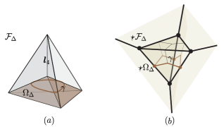
Figure 16: Suppose we have a 3-dimensional curved manifold $\mathcal{F}_{\triangle}$ discretized by four tetrahedron in the figure (a) (in flat case it is known as 1-4 Pachner move). Then we take an embedded slice $\Omega_{\triangle}$ as the surface of one tetrahedron (the dark blue surface discretized by three triangle). Embedded on $\Omega_{\triangle},$ we take a loop $\gamma$ circling a point of a tetrahedron. Attached to $\gamma$, are the $SU(2)$ and $SO(2)$ holonomy, which are related to the 3D and 2D intrinsic curvature, respectively. (b) is the dual lattice of (a). The use of abstract combinatorial dual guarantees $\star\Omega_{\Delta}$ to be embedded in $\star\mathcal{F}.$

The first step is to define the holonomy of the projected 3-dimensional and 2-dimensional intrinsic curvature along the loop. The following are several quantities we had on the simplicial complex, each of them will be illustrated geometrically on the primal and dual lattices.

IV.4.2 The Curvatures

Projected 3D intrinsic curvature: deficit angle on segment $\boldsymbol{l}_{4}$.

Loop $\gamma_{4}$ circles hinges $\boldsymbol{l}_{1}$, $\boldsymbol{l}_{2}$, and $\boldsymbol{l}_{3}$, and therefore, the total 3-dimensional holonomy on $\gamma_{4}$ is the product of holonomies on each hinge it contains. By (25), it is clear that the 3-dimensional holonomy around loop $\gamma_{4}$ on $\Omega_{4}$ with origin $\mathcal{O}=\star\boldsymbol{v}_{4}$, is:

$$\boldsymbol{H}_{123}\left(\boldsymbol{A},\gamma_{4,\mathcal{O}}\right)=\boldsymbol{H}_{42}\boldsymbol{H}_{4}^{-1}\boldsymbol{H}_{24}.$$

Therefore, the projected 3D intrinsic curvature on $\Omega_{4}$ in the holonomy representation, is:

$$\left.\,{}^{3}\boldsymbol{F}_{\Delta}\right|_{\Sigma}=\boldsymbol{H}_{123}\left(\boldsymbol{A},\gamma_{4,\mathcal{O}}\right).$$

Written in the plane-angle representation, we have the deficit angle and plane which are functions of $\delta\theta_{i},\boldsymbol{l}_{i}$, $i=1,2,3$ by the closure constraint (24):

$\displaystyle\left.\,{}^{3}\boldsymbol{F}_{\Delta}\right|_{\Sigma}$ $\displaystyle=$ $\displaystyle\left(\delta\theta_{4},\left.\hat{\boldsymbol{J}}_{4}\right|_{\mathcal{O}}\right)=\left(\delta\theta_{4},\boldsymbol{H}_{42}\left.\frac{d\boldsymbol{H}_{4}}{d\delta\theta_{4}}\right|_{\delta\theta_{4}=0}\boldsymbol{H}_{24}\right),$ $\displaystyle\delta\theta_{4}$ $\displaystyle=$ $\displaystyle 2\pi-\left(\theta_{ij,4}+\theta_{ik,4}+\theta_{jk,4}\right),\,i,j,k\neq 4,i<j<k,$ $\displaystyle\left.\hat{\boldsymbol{J}}_{4}\right|_{\mathcal{O}}$ $\displaystyle=$ $\displaystyle\left.\frac{d\boldsymbol{\overline{H}}_{4}}{d\delta\theta_{4}}\right|_{\delta\theta_{4}=0}.$

see FIG. 17.

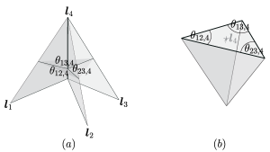
Figure 17: a) the projected 3D intrinsic curvature in primal lattice, (b) the projected 3D intrinsic curvature in dual lattice.

2D intrinsic curvature: deficit angle on point $p$.

It is clear from (39) that the 2-dimensional holonomy around loop $\gamma_{4}$ on $\Omega_{4}$ with origin $\mathcal{P}$, is:

$$\,{}^{2}\boldsymbol{F}_{\triangle}=\boldsymbol{O}_{4}\left(\boldsymbol{a},\gamma_{4,\mathcal{P}}\right),$$

with the plane-angle representation as:

$\,{}^{2}\boldsymbol{F}_{\Delta}$ $\displaystyle=$ $\displaystyle\left(\delta\phi_{4},\left.\boldsymbol{\hat{j}}_{4}\right|_{\mathcal{P}}\right),$ $\displaystyle\delta\phi_{4}$ $\displaystyle=$ $\displaystyle 2\pi-\left(\phi_{ij}+\phi_{ik}+\phi_{jk}\right),\,i,j,k\neq 4,i<j<k,$

see FIG. 18.

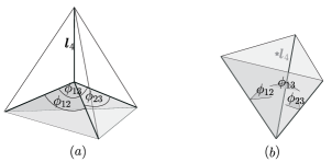
Figure 18: (a) the 2D intrinsic curvature in primal lattice, (b) the 2D intrinsic curvature in dual lattice.

2D extrinsic curvature.

The total extrinsic curvature circling loop $\gamma_{4}$ on slice $\Omega_{4}$ with origin $\mathcal{O}$, is the product of $\boldsymbol{\mathcal{K}}_{i}$ on the three hinge it crosses:

$$\boldsymbol{\mathcal{K}}_{123}=\boldsymbol{\mathcal{K}}_{1}\boldsymbol{\mathcal{K}}_{2}\boldsymbol{\mathcal{K}}_{3},$$

Each $\boldsymbol{\mathcal{K}}_{i}$ satisfies (46) and (48), where each external dihedral angles, from (45), are:

$$\bar{\theta}_{i}=\theta_{j4,i}+\theta_{k4,i},\qquad i,j,k=1,2,3,\>i\neq j\neq k,$$ (50)

see FIG. 19.

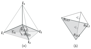
Figure 19: (a) the 2D extrinsic curvature in primal lattice, (b) the 2D extrinsic curvature in dual lattice.

Therefore, the 2D extrinsic curvature, written in holonomy and plane-angle representation, are:

$$\,{}^{2}\boldsymbol{K}_{\triangle} = \boldsymbol{\mathcal{K}}_{123}\left(\gamma_{4,\mathcal{O}}\right),$$

$$\,{}^{2}\boldsymbol{K}_{\Delta} = \left(\delta\kappa_{123}\sim\textrm{tr $\boldsymbol{\mathcal{K}}_{123}$},\left.\frac{d\boldsymbol{\mathcal{K}}_{123}}{d\delta\kappa_{123}}\right|_{\delta\kappa_{123}=0}\right)$$

These definitions of discrete curvatures are natural, in the sense that we did not use any assumption to derive them, besides the assumption of small loop approximation. An important fact that arise from these definition is that the extrinsic and intrinsic curvature can not be obtained simultaneously; which will be clear in the next subsection.

IV.4.3 Dihedral Angle Relation as the Discrete Gauss-Codazzi Equation

To derive the Gauss-Codazzi equation, we need these following quantities: 3D curvature, 2D curvature, and the Bianchi identity. The holonomies of these three quantities have different ’natural’ points of origin; the origin $\mathcal{O}$ of 3D holonomy is naturally located at the vertex, the origin $\mathcal{P}$ of 2D holonomy at (the middle of) the face, while the origin $\mathcal{O}^{\prime}$ of the trivalent loops on (the middle of) the edge. To obtain the correct relation, all of them need to have a same origin. The following transformation of an arbitrary holonomy $\boldsymbol{H}_{\gamma}$ on loop $\gamma$ will be useful:

$$\boldsymbol{H}_{\gamma}\left(\gamma_{\mathcal{P}}\right)=\boldsymbol{O}_{ik}^{\left(R\right)-1}\boldsymbol{H}_{\gamma}\left(\gamma_{\mathcal{O}^{\prime}}\right)\boldsymbol{O}_{ik}^{\left(R\right)}=\boldsymbol{O}_{ik}^{\left(R\right)-1}\boldsymbol{H}_{lj}^{\left(R\right)}\boldsymbol{H}_{\gamma}\left(\gamma_{\mathcal{O}}\right)\boldsymbol{H}_{lj}^{\left(R\right)-1}\boldsymbol{O}_{ik}^{\left(R\right)}.$$ (51)

See FIG. 14(a).

From the discrete Bianchi identity, we could write:

$$\boldsymbol{h}_{ij,k}\left(\boldsymbol{A},\gamma_{k,\mathcal{O}^{{}^{\prime}}}\right)=\boldsymbol{h}_{kj,i}\left(\boldsymbol{A},\gamma_{i,\mathcal{O}^{{}^{\prime}}}\right)\boldsymbol{h}_{ik,j}\left(\boldsymbol{A},\gamma_{j,\mathcal{O}^{{}^{\prime}}}\right),$$ (52)

with point $\mathcal{O}^{\prime}$ as the origin. There exist a beautiful geometrical interpretation of relation (52) as follows. Since they are 3D holonomies, $\boldsymbol{h}_{ij,k}$’s are elements of $SU\left(2\right)$, and therefore, could be written explicitly by (18). Taking the trace of (52), gives exactly the following relation:

$$\cos\theta_{ij,k}=\cos\theta_{ik,j}\cos\theta_{kj,i}-\cos\bar{\phi}_{ij}\sin\theta_{ik,j}\sin\theta_{kj,i},$$ (53)

which is indeed the total angle relation formula (19). The $\theta_{ij,k}$’s are the angle of rotation of holonomy $\boldsymbol{h}_{ij,k}$’s, while $\bar{\phi}_{ij}$ is the angle between plane of rotation $\hat{\boldsymbol{J}}_{i}$ and $\hat{\boldsymbol{J}}_{j}$:

$$\left.\hat{\boldsymbol{J}}_{i}\right|_{\mathcal{O}^{{}^{\prime}}} = \left.\frac{d\boldsymbol{h}_{kj,i}}{d\theta_{kj,i}}\right|_{d\theta_{kj,i}=0},$$

$$\left.\hat{\boldsymbol{J}}_{j}\right|_{\mathcal{O}^{{}^{\prime}}} = \left.\frac{d\boldsymbol{h}_{ik,j}}{d\theta_{ik,j}}\right|_{d\theta_{ik,j}=0},$$

which are (28) parallel-transported to $\mathcal{O}^{{}^{\prime}}$ (remember that $\boldsymbol{H}_{k}$ and $\boldsymbol{h}_{ij,k}$ share the same hinge $\boldsymbol{l}_{k},$and therefore share the same plane of rotation $\boldsymbol{J}_{k}$, but different angle of rotation). In the vectorial picture viewed from $\mathcal{O}^{\prime}$, plane of rotation $\boldsymbol{J}_{i}$ and $\boldsymbol{J}_{j}$ are indeed dual to segment $\boldsymbol{l}_{i}$ and $\boldsymbol{l}_{j}$. With $\phi_{ij}=\pi-\bar{\phi}_{ij}$ as the angle between hinge $\boldsymbol{l}_{i}$ and $\boldsymbol{l}_{j}$, we could write (53) as the dihedral angle formula, which is a relation between $\phi$, the 2D angles between segments of a Euclidean tetrahedron, and $\theta,$ the 3D angles between planes of the same tetrahedron:

$$\cos\phi_{ij}=\frac{\cos\theta_{ij,k}-\cos\theta_{ik,j}\cos\theta_{kj,i}}{\sin\theta_{ik,j}\sin\theta_{kj,i}}.$$ (54)

see FIG. 20.

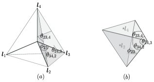
Figure 20: (a) Given angles $\phi_{ij}$, $\phi_{ik}$, $\phi_{jk}$ at point $p$ of a tetrahedron, we could obtain the dihedral angle $\theta{}_{ij,k}$. In fact, $\theta{}_{ij,k}$ is only $\phi_{ij}$ projected on the plane normal to segment $\boldsymbol{l}_{k}$. (b) In the dual lattice.

Remarkably, as shown in key-59 , the dihedral angle formula is valid for any dimension, relating $p$-dimensional angle (the angle between $\left(p-1\right)$-simplices) with $\left(p-1\right)$-dimensional angle (the angle between $\left(p-2\right)$-simplices). The formula can also be written in the inverse form:

$$\cos\theta{}_{ij,k}=\frac{\cos\phi{}_{ij}-\cos\phi_{ik}\cos\phi_{kj}}{\sin\phi_{ik}\sin\phi_{kj}},$$ (55)

We will show that this formula is the discrete Gauss-Codazzi relation for angles, which will give the continuous Gauss-Codazzi relation (10) in the continuum limit.

Since $\theta_{ij,k}$ and $\phi_{ij}$ are, respectively, the parts of 3D and 2D intrinsic curvature, the dihedral angle formula relates these intrinsic curvatures together. Therefore, it is reasonable to expect the remaining term to be the extrinsic curvature; we will check if it coincides with our definition in (48).

The next step, is to write the elements of 3D and 2D curvature in the point of view of $\mathcal{O}^{\prime}$ as the origin. For the 3D curvature, it is done by equation (32), while for 2D, it is done by (40). Returning to relation (52), an important remarks we need to emphasize is: the $\boldsymbol{h}$’s are the holonomy circling segments, which is a 3-dimensional properties. The 2-dimensional property $\bar{\phi}_{ij}$ comes implicitly from the relation between two 3D holonomies $\boldsymbol{h}_{kj,i}$ and $\boldsymbol{h}_{ik,j}$. We could explicitly insert the 2-dimensional property by gauge fixing: sending one of the holonomy, say $\boldsymbol{h}_{kj,i}$ at hinge $\boldsymbol{l}_{i}$ to $\boldsymbol{l}_{j}$. The corresponding 2D holonomy connecting these two hinges is:

$$\boldsymbol{O}_{ij}=\boldsymbol{O}_{ij}\left(\boldsymbol{a},\gamma_{\mathcal{P}}\right)=\exp\left(\left.\frac{d\boldsymbol{O}_{ij}}{d\phi_{ij}}\right|_{\phi_{ij}=0}\phi_{ij}\right),$$

which can be written in $\mathcal{O}^{{}^{\prime}}$ point of view, using transformation (51):

$$\boldsymbol{O}_{ij}^{{}^{\prime}} = \boldsymbol{O}_{ij}^{{}^{\prime}}\left(\boldsymbol{a},\gamma_{\mathcal{O}^{\prime}}\right)=\exp\left(\boldsymbol{O}^{\left(R\right)}\left.\frac{d\boldsymbol{O}_{ij}}{d\phi_{ij}}\right|_{\phi_{ij}=0}\boldsymbol{O}^{\left(R\right)-1}\phi_{ij}\right).$$ (56)

Relation (52) can be rewritten as:

$$\boldsymbol{h}_{ij,k}\left(\boldsymbol{A},\gamma_{\mathcal{O}^{\prime}}\right)=\boldsymbol{O}_{ij}^{{}^{\prime}}\left(\boldsymbol{a},\gamma_{\mathcal{O}^{\prime}}\right)\underset{\boldsymbol{h}_{kj,i}^{{}^{\prime}}\left(\boldsymbol{A},\gamma_{\mathcal{O}^{\prime}}\right)}{\underbrace{\boldsymbol{O}_{ij}^{{}^{\prime}-1}\left(\boldsymbol{a},\gamma_{\mathcal{O}^{\prime}}\right)\boldsymbol{h}_{kj,i}\left(\boldsymbol{A},\gamma_{\mathcal{O}^{\prime}}\right)\boldsymbol{O}_{ij}^{{}^{\prime}}\left(\boldsymbol{a},\gamma_{\mathcal{O}^{\prime}}\right)}}\boldsymbol{O}_{ij}^{{}^{\prime}-1}\left(\boldsymbol{a},\gamma_{\mathcal{O}^{\prime}}\right)\boldsymbol{h}_{ik,j}\left(\boldsymbol{A},\gamma_{\mathcal{O}^{\prime}}\right).$$ (57)

with:

$$\boldsymbol{h}_{kj,i}^{{}^{\prime}} = \boldsymbol{O}_{ij}^{{}^{\prime}-1}\boldsymbol{h}_{kj,i}\boldsymbol{O}_{ij}^{{}^{\prime}}=\boldsymbol{O}_{ij}^{{}^{\prime}-1}\exp\left(\left.\boldsymbol{J}_{i}\right|_{\mathcal{O}^{{}^{\prime}}}\theta_{kj,i}\right)\boldsymbol{O}_{ij}^{{}^{\prime}},$$ (58)

$$= \exp\left(\boldsymbol{O}_{ij}^{{}^{\prime}-1}\left.\boldsymbol{J}_{i}\right|_{\mathcal{O}^{{}^{\prime}}}\boldsymbol{O}_{ij}^{{}^{\prime}}\theta_{kj,i}\right),$$

$$= \exp\left(\left.\boldsymbol{J}_{j}\right|_{\mathcal{O}^{{}^{\prime}}}\theta_{kj,i}\right).$$

$\boldsymbol{h}_{kj,i}^{{}^{\prime}}$ is the holonomy $\boldsymbol{h}_{kj,i}$ at hinge $\boldsymbol{l}_{i}$, sent to $\boldsymbol{l}_{j}$. Therefore, (57) can be written as:

$$\boldsymbol{h}_{ij,k}\left(\boldsymbol{A},\gamma_{\mathcal{O}^{\prime}}\right)=\boldsymbol{O}_{ij}^{{}^{\prime}}\left(\boldsymbol{a},\gamma_{\mathcal{O}^{\prime}}\right)\boldsymbol{h}_{kj,i}^{{}^{\prime}}\left(\boldsymbol{A},\gamma_{\mathcal{O}^{\prime}}\right)\boldsymbol{O}_{ij}^{{}^{\prime}-1}\left(\boldsymbol{A},\gamma_{\mathcal{O}^{\prime}}\right)\boldsymbol{h}_{ik,j}\left(\boldsymbol{A},\gamma_{\mathcal{O}^{\prime}}\right),$$ (59)

with $\boldsymbol{O}{}_{ij}^{{}^{\prime}}$ satisfying (56) and $\boldsymbol{h}_{kj,i}^{{}^{\prime}}$ satisfying (58).

If $\boldsymbol{h}_{ij,k}$ and $\boldsymbol{O}_{ij}^{{}^{\prime}}$ describe the 3D and 2D intrinsic curvature, then the extrinsic curvature term should be:

$$\boldsymbol{\mathcal{K}}_{ij,k}\left(\gamma_{\mathcal{O}^{\prime}}\right)=\boldsymbol{h}_{kj,i}^{{}^{\prime}}\boldsymbol{O}_{ij}^{{}^{\prime}-1}\boldsymbol{h}_{ik,j},$$ (60)

which define the extrinsic curvature of triangle $\boldsymbol{a}_{ij}$, located at $\boldsymbol{l}_{i}$. (59) can be written as:

$$\boldsymbol{h}_{ij,k}=\boldsymbol{O}_{ij}^{{}^{\prime}}\boldsymbol{\mathcal{K}}_{ij,k}.$$ (61)

Notice that $\boldsymbol{\mathcal{K}}_{ij,k}$ and $\boldsymbol{O}_{ij}^{{}^{\prime}}$ do not commute in general. Another way of writting (61) exist, which is a consequence of the freedom in choosing the order of $\boldsymbol{\mathcal{K}}_{ij,k}$ and $\boldsymbol{O}_{ij}^{{}^{\prime}}$, and the freedom in choosing a fixed hinge $\boldsymbol{l}_{i}$ or $\boldsymbol{l}_{j}$.

If (53) is the discrete Gauss-Codazzi in terms of angle, then (61) is the discrete Gauss-Codazzi in terms of holonomy. It must be kept in mind that (61) is not the Gauss-Codazzi equation on a full loop $\gamma$, but on the third half of the loop (or the red tetrahedral lattice in FIG. 12(b)).

Now let us check if $\boldsymbol{\mathcal{K}}_{ij,k}$ coincides with our definition of extrinsic curvature $\boldsymbol{\mathcal{K}}_{i\Delta}$ in (48), or at least, with the external dihedral angle $\bar{\theta}_{i}$ in (50). Taking trace of (60) (and using the fact that $\textrm{tr}ABC=\textrm{tr}CAB,$ together with equation (18), (19), and some trigonometric identities) gives:

$$\cos\kappa_{ij,k}=\cos\left(\underset{\theta_{j}^{{}^{\prime}}}{\underbrace{\theta_{ik,j}+\theta_{kj,i}}}\right)\cos\phi_{ij}.$$ (62)

Comparing (50) and (62), it is clear that they are not equivalent, with the geometrical picture illustrated in FIG. 21 as follows.

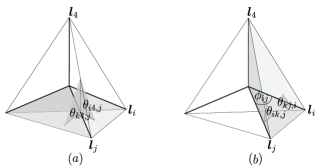
Figure 21: (a) The discrete extrinsic curvature from its continuous counterpart, (50), (b) The extrinsic curvature from discrete Gauss-Codazzi equation, (62).

The discrepancy is caused by the different natural location of the extrinsic and intrinsic curvature. The extrinsic curvature is located naturally on segment $\boldsymbol{l}$ (FIG. 21(a), where the extrinsic curvature is defined by the external angle $\bar{\theta}$ of (50)), while the 2D intrinsic curvature lies naturally on point $p$. Since the Gauss-Codazzi relation needs to be defined on a same (part) of the loop, the extrinsic curvature is forced to be located at a same place where the intrinsic curvature lies. This is illustrated in FIG. 21(b), where the extrinsic curvature is defined by angle $\theta^{{}^{\prime}}$ of (62), on different hinge $i,j$, which defines the tetrahedron. The factor $\cos\phi_{ij}$ describe the relation between different parts of extrinsic curvature. It is impossible to obtain the intrinsic and extrinsic curvature simultaneously, in the sense, the sharpness of one of them will cause the spread in other, since they live in different hinges. This ’non-commutativity’ occurs because of the discreteness. Nevertheless, it is clear that if we refine the discretization, in the continuum limit where $\phi\rightarrow 0$, the tetrahedron will shrink to a single point, thus the intrinsic and extrinsic curvature will be located on the same place and $\bar{\theta}\approx\theta^{{}^{\prime}}$. The ’non-commutativity’ between the quantities will dissapear.

V The Continuum Limit and Discussions

V.1 Recovering the Continuum Limit

Let us collect all together the results obtained from the previous sections in the following table:

2D discrete curvature 2-form	$\,{}^{2}\boldsymbol{F}_{\triangle}=\boldsymbol{O}_{4}\left(\boldsymbol{a},\lambda_{4,\mathcal{P}}\right)$
3D discrete curvature 2-form	$\,{}^{3}\boldsymbol{F}_{\triangle}=\left(\boldsymbol{H}_{1}\left(\boldsymbol{A},\gamma_{1,\mathcal{O}}\right),\boldsymbol{H}_{2}\left(\boldsymbol{A},\gamma_{2,\mathcal{O}}\right),\boldsymbol{H}_{3}\left(\boldsymbol{A},\gamma_{3,\mathcal{O}}\right)\right).$
Closure constraint	$\boldsymbol{H}_{1}\left(\boldsymbol{A},\gamma_{1,\mathcal{O}}\right)\boldsymbol{H}_{2}\left(\boldsymbol{A},\gamma_{2,\mathcal{O}}\right)\boldsymbol{H}_{3}\left(\boldsymbol{A},\gamma_{3,\mathcal{O}}\right)\overline{\boldsymbol{H}}_{4}\left(\boldsymbol{A},\gamma_{4,\mathcal{O}}\right)=\boldsymbol{1},$
Bianchi identity	$\boldsymbol{h}_{kl,i}\left(\boldsymbol{A},\gamma_{i,\mathcal{O}^{{}^{\prime}}}\right)\boldsymbol{h}_{ik,l}\left(\boldsymbol{A},\gamma_{l,\mathcal{O}^{{}^{\prime}}}\right)\boldsymbol{h}_{li,k}\left(\boldsymbol{A},\gamma_{k,\mathcal{O}^{{}^{\prime}}}\right)=1,$
Gauss-Codazzi equation	$\boldsymbol{h}_{ij,k}\left(\boldsymbol{A},\gamma_{i,\mathcal{O}^{{}^{\prime}}}\right)=\boldsymbol{O}_{ij}^{{}^{\prime}}\left(\boldsymbol{A},\gamma_{i,\mathcal{O}^{{}^{\prime}}}\right)\boldsymbol{\mathcal{K}}_{ij,k}\left(\boldsymbol{A},\gamma_{i,\mathcal{O}^{{}^{\prime}}}\right).$

Table 1: The discrete geometrical quantities and relations.

We will show that these discrete geometrical variables and relations will yield their standard infinitesimal and continuous counterparts.

V.1.1 Recovering the Infinitesimal Curvature 2-Form

The 3D discrete curvature 2-form is written as follows:

$$\left(\,{}^{3}\boldsymbol{F}_{\triangle}\right)_{\mu\nu}=\boldsymbol{H}_{\mu\nu}\left(\boldsymbol{A},\gamma_{\mu\nu,\mathcal{O}}\right)=\left(\boldsymbol{H}_{1}\left(\boldsymbol{A},\gamma_{1,\mathcal{O}}\right),\boldsymbol{H}_{2}\left(\boldsymbol{A},\gamma_{2,\mathcal{O}}\right),\boldsymbol{H}_{3}\left(\boldsymbol{A},\gamma_{3,\mathcal{O}}\right)\right),$$ (63)

where we recover the indices $\mu\nu$ which had been dropped for simplicity in the previous section. The first step is to expand (63) near the origin $\mathcal{O}$ in the direction $\ell dx^{\mu}\times\ell dx^{\nu}$. By relation (13), the holonomies can be written as:

$$\boldsymbol{H}_{\mu\nu}\left(\boldsymbol{A},\gamma_{a,\mathcal{O},\partial_{\mu}\partial_{\nu}}\right)=1+\frac{\ell^{2}}{2}\boldsymbol{F}\left(\partial_{\mu},\partial_{\nu}\right)+O\left(\ell^{3}\right).$$

Therefore, (63) can be written as:

$$\left(\,{}^{3}\boldsymbol{F}_{\triangle}\right)_{\mu\nu} = 1+\frac{\ell^{2}}{2}\boldsymbol{F}\left(\partial_{\mu},\partial_{\nu}\right)+O\left(\ell^{3}\right),$$

$$= \left(1+\frac{\ell^{2}}{2}\boldsymbol{F}\left(\partial_{2},\partial_{3}\right)+O\left(\ell^{3}\right),1+\frac{\ell^{2}}{2}\boldsymbol{F}\left(\partial_{3},\partial_{1}\right)+O\left(\ell^{3}\right),1+\frac{\ell^{2}}{2}\boldsymbol{F}\left(\partial_{1},\partial_{2}\right)+O\left(\ell^{3}\right)\right).$$

Taking only the first order terms, which is equivalent with taking a small loop by setting $\ell\ll 1$, we have:

$$\left(\,{}^{3}\boldsymbol{F}_{\triangle}\right)_{\mu\nu}\approx 1+\frac{\ell^{2}}{2}\boldsymbol{F}\left(\partial_{\mu},\partial_{\nu}\right)=\left(1+\frac{\ell^{2}}{2}\boldsymbol{F}\left(\partial_{2},\partial_{3}\right),1+\frac{\ell^{2}}{2}\boldsymbol{F}\left(\partial_{3},\partial_{1}\right),1+\frac{\ell^{2}}{2}\boldsymbol{F}\left(\partial_{1},\partial_{2}\right)\right).$$

Now, to take the continuum limit, we differentiate $\,{}^{3}\boldsymbol{F}_{\triangle}$ with respect to a parameter, which we choose to be the norm of the vector, $\ell$. This is analog to a differentiation of a curve by a differential operator to obtain a vector:

$$\frac{d\left(\,{}^{3}\boldsymbol{F}_{\triangle}\right)_{\mu\nu}}{d\ell}\approx\ell\boldsymbol{F}\left(\partial_{\mu},\partial_{\nu}\right)=\ell\left(\boldsymbol{F}\left(\partial_{2},\partial_{3}\right),\left(\partial_{3},\partial_{1}\right),\left(\partial_{1},\partial_{2}\right)\right).$$ (64)

Moreover, (64) can be written as:

$$\frac{1}{\ell}\frac{d\,^{3}\boldsymbol{F}_{\triangle}}{d\ell}\approx\boldsymbol{F}.$$ (65)

with $\,{}^{3}\boldsymbol{F}_{\triangle}$ is the discrete curvature 2-form and $\boldsymbol{F}$ is its continuous counterpart. The same procedure could be applied to $\,{}^{2}\boldsymbol{F}_{\triangle}$ and $\,{}^{2}\boldsymbol{K}_{\triangle}$.

V.1.2 Recovering the Closure Constraint of a Flat Tetrahedron

The generalized closure constraint:

$$\boldsymbol{H}_{1}\boldsymbol{H}_{2}\boldsymbol{H}_{3}\overline{\boldsymbol{H}}_{4}=1,$$ (66)

guarantees the closure of, in general, a curved tetrahedron key-67 . For a special case where the gauge group $\mathcal{G}=SU\left(2\right)$, (66) can be written in the plane-angle representation using (18), which in general, does not gives zero for the total summations of the planes. But according to key-29 ; key-67 , in a small loop approximation, the Taylor expansion of (11), will give:

$$\boldsymbol{H}\left(\boldsymbol{A},\gamma_{\mathcal{O},\ell}\right)=\boldsymbol{1}+\ell\boldsymbol{A}+O\left(\ell^{2}\right),$$ (67)

such that (66) gives the closure of a flat tetrahedron:

$$\sum_{i=1}^{4}\boldsymbol{A}_{i}=0,$$ (68)

with $\boldsymbol{A}_{i}$ define the hinges of a flat 4-1 Pachner move.

Let us take one of the planes in (68), say $\boldsymbol{A}_{4}$, to be zero. This will give:

$$\sum_{i=1}^{3}\boldsymbol{A}_{i}=0,$$ (69)

which is geometrically interpreted as a closure of a flat triangle. Thus we could conclude that a special case of (68), where one of the plane is trivial, is a condition for a flat tetrahedron with a zero volume, practically, a flat triangle. Now let us take a special case of (66), where one of the holonomy, say $\overline{\boldsymbol{H}}_{4}$, is trivial. This gives: $\boldsymbol{H}_{1}\boldsymbol{H}_{2}\boldsymbol{H}_{3}=1,$ which is the Bianchi identity. Following the analogy with the small loop approximation case, a special case of (66), where one of the holonomy is trivial, is a condition for a curved tetrahedron with a zero volume: a curved triangle. But a curved triangle can always be constructed from three flat triangles meeting one another on their segments, which is an open portion of a surface of a flat tetrahedron.

Another fact which strengthen our claim is, (69), which can be written as $-\boldsymbol{A}_{3}=\boldsymbol{A}_{1}+\boldsymbol{A}_{2},$ gives:

$$\left|\boldsymbol{A}_{3}\right|^{2}=\left|\boldsymbol{A}_{1}+\boldsymbol{A}_{2}\right|^{2}=\left|\boldsymbol{A}_{1}\right|^{2}+\left|\boldsymbol{A}_{2}\right|^{2}+2\left\langle\boldsymbol{A}_{1},\boldsymbol{A}_{2}\right\rangle,$$ (70)

as their norms relation (by taking traces), which is clearly the flat law of cosine. The curved version of this, is remarkably the trace of Bianchi identity, namely relation (53), which is the spherical law of cosine. Taking small angle (which is equivalent with taking small loop) approximation, (53) becomes:

$$\theta_{ij,k}^{2}\approx\theta_{ik,j}^{2}+\theta_{kj,i}^{2}+2\theta_{ik,j}\theta_{kj,i}\cos\bar{\phi}_{ij},$$

which is clearly the flat law of cosine in the form of (70).

V.1.3 Recovering the Bianchi Identity

Let us consider the tetrahedral lattice in FIG. 11(a) and 12(b). Since we assume the tetrahedra are flat in the interior, relation (34) is satisfied, and the generalized closure constraint reduces to Bianchi identity, which we rewrite as follows:

$$\boldsymbol{h}_{\mu\nu,\lambda}\boldsymbol{h}_{\lambda\mu,\nu}\boldsymbol{h}_{\nu\lambda,\mu}=1.$$ (71)

The total holonomy $P_{j}$ is trivial so that the loop can be shrunk into a point, such that it gives lattice in FIG. 22(b).

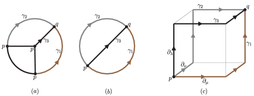
Figure 22: (a). A tetrahedral lattice where one of the four loop has trivial holonomy such that it can be shrunk to a point $p$. (b) Figure (a) is topologically equivalent with (b). (c) Figure (b) is topologically equivalent with (c).

FIG. 22(a), usually called as the theta-graph key-22 , is topologically equivalent to holonomies on the segments of the cube, see FIG. 22(c). Let us define the holonomies on the segments of the cube as follows, see FIG. 23.

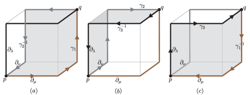
Figure 23: Three path of the holonomies on the bones of the cube.

The holonomy on path $\gamma_{\mu}\gamma_{\nu}^{-1}$ is written as:

$$\boldsymbol{h}_{\mu\nu,\lambda}=\boldsymbol{h}_{\mu\nu,\lambda}\left(\boldsymbol{A},\gamma_{\mu}\gamma_{\nu,\mathcal{O}^{{}^{\prime}}}^{-1}\right).$$

For path $\gamma_{\mu}\gamma_{\nu}^{-1}$ , the holonomy could be Taylor expand near point $p$, in the direction of plane $\ell dx^{\mu}\times\ell dx^{\nu}$, up to the third order, as:

$$\boldsymbol{h}_{\mu\nu,\lambda}\left(\boldsymbol{A},\gamma_{\mu}\gamma_{\nu,\mathcal{O}^{{}^{\prime}},\partial_{\mu}\partial_{\nu}}^{-1}\right)=1-\frac{\ell^{2}}{2}F_{\mu\nu}+\frac{\ell^{2}}{2}F_{\nu\lambda}+\frac{\ell^{3}}{3!}D_{\nu}F_{\lambda\mu}+O\left(\ell^{4}\right).$$

It is clear that the holonomies on the three paths in FIG. 21 satisfy the Bianchi identity (71). Inserting the expansion to the discrete Bianchi identity yields:

$$\boldsymbol{h}_{\mu\nu,\lambda}\boldsymbol{h}_{\lambda\mu,\nu}\boldsymbol{h}_{\nu\lambda,\mu}=1+\frac{\ell^{3}}{3!}\left(D_{\mu}F_{\nu\lambda}+D_{\nu}F_{\lambda\mu}+D_{\lambda}F_{\mu\nu}\right)+O\left(\ell^{4}\right)=1.$$

Taking the small loop limit, which is equal with neglecting the terms up to the fourth order, gives:

$$1+\frac{\ell^{3}}{3!}\left(D_{\mu}F_{\nu\lambda}+D_{\nu}F_{\lambda\mu}+D_{\lambda}F_{\mu\nu}\right)\approx 1,$$

or:

$$\left(D_{\mu}F_{\nu\lambda}+D_{\nu}F_{\lambda\mu}+D_{\lambda}F_{\mu\nu}\right)\approx 0,$$

which is exactly relation (3), or geometrically, (2). (3) could also be written as the Jacobi identity:

$$\left[D_{\mu},\left[D_{\nu},D_{\lambda}\right]\right]+\left[D_{\nu},\left[D_{\lambda},D_{\mu}\right]\right]+\left[D_{\lambda},\left[D_{\mu},D_{\nu}\right]\right]=0.$$

The geometrical interpretation of Jacobi identity is the altitude of a trihedron have three planes meeting in a line key-1.14 , which guarantees the flat law of cosine to be satisfied for a triangle. This is in accordance with the fact that the Bianchi identity for angles (53) is indeed the dihedral angle relation, or the spherical law of cosine, which is satisfied by a curved triangle.

V.1.4 Recovering the Gauss-Codazzi equation

Let us take the discrete Gauss-Codazzi relation (61) as follows:

$$\boldsymbol{h}_{ij,k}\left(\boldsymbol{A},\gamma_{i,\mathcal{O}^{{}^{\prime}}}\right)=\boldsymbol{O}_{ij}^{{}^{\prime}}\left(\boldsymbol{A},\gamma_{i,\mathcal{O}^{{}^{\prime}}}\right)\boldsymbol{\mathcal{K}}_{ij,k}\left(\boldsymbol{A},\gamma_{i,\mathcal{O}^{{}^{\prime}}}\right).$$

This relation is defined only on a third half part of loop $\gamma_{4}$. To obtain the full relation on loop $\gamma_{4}$, one need to take the piecewise linear product of all parts of $\gamma_{4}$. Following relation (32), the total 3D holonomy on $\gamma_{4}$ is:

$$\left.\,{}^{3}\boldsymbol{H}\right|_{\Sigma_{4}}=\boldsymbol{h}_{ij,4}\boldsymbol{h}_{jl,4}\boldsymbol{h}_{li,4}.$$

Inserting the Gauss-Codazzi relation (61) to the previous equation, we have:

$$\left.\,{}^{3}\boldsymbol{H}\right|_{\Sigma_{4}}=\boldsymbol{O}_{ij}^{{}^{\prime}}\boldsymbol{\mathcal{K}}_{ij,4}\boldsymbol{O}_{jl}^{{}^{\prime}}\boldsymbol{\mathcal{K}}_{jl,4}\boldsymbol{O}_{li}^{{}^{\prime}}\boldsymbol{\mathcal{K}}_{li,4}.$$ (72)

Notice that it is impossible to explicitly obtain $\left.\,{}^{3}\boldsymbol{H}\right|_{\Sigma}$ simultaneously as a function of $\boldsymbol{O}$ or/and $\boldsymbol{\mathcal{K}}$, where:

$$\boldsymbol{O}^{{}^{\prime}} = \boldsymbol{O}^{\prime}_{ij}\boldsymbol{O}^{\prime}_{jl}\boldsymbol{O}^{\prime}_{li},$$

$$\boldsymbol{\mathcal{K}} = \boldsymbol{\mathcal{K}}_{ij,4}\boldsymbol{\mathcal{K}}_{jl,4}\boldsymbol{\mathcal{K}}_{li,4}.$$

because of the non-commutativity between $\boldsymbol{O}_{ij}^{{}^{\prime}}$ and $\boldsymbol{\mathcal{K}}_{ij,4}$.

But as explained earlier, taking the continuum limit, i.e., taking small loop approximation, will give simplification. Using (15) and (44), we can write (72) as:

$$\boldsymbol{1}-\frac{\ell^{2}}{2}\left.\,{}^{3}\boldsymbol{F}\right|_{\Sigma}+O\left(\ell^{3}\right)=\prod_{l=1}^{3}\left(1-\frac{\ell^{2}}{2}\,^{2}\boldsymbol{F}_{l}+O\left(\ell^{3}\right)\right)\left(1-\frac{\ell^{2}}{2}\boldsymbol{k}_{l}+O\left(\ell^{3}\right)\right),$$

where:

$$\,{}^{2}\boldsymbol{F}_{l} = \,{}^{2}\boldsymbol{F}\left(\hat{\boldsymbol{s}}_{i},\hat{\boldsymbol{s}}_{j}\right),\quad l\neq i,j,k.$$

$$\boldsymbol{k}_{l} = \left[\mathcal{\boldsymbol{K}}_{l},\mathcal{\boldsymbol{K}}_{l}\right].$$

Neglecting up to the third order terms (which is equivalent with using small loop) gives:

$$\boldsymbol{1}-\ell^{2}\left.\,{}^{3}\boldsymbol{F}\right|_{\Sigma}\approx 1-\ell^{2}\left(\left[\mathcal{\boldsymbol{K}}_{1},\mathcal{\boldsymbol{K}}_{1}\right]+\left[\mathcal{\boldsymbol{K}}_{2},\mathcal{\boldsymbol{K}}_{2}\right]+\left[\mathcal{\boldsymbol{K}}_{3},\mathcal{\boldsymbol{K}}_{3}\right]\right)-\ell^{2}\left(\,{}^{2}\boldsymbol{F}\left(\hat{\boldsymbol{s}}_{1},\hat{\boldsymbol{s}}_{2}\right)+\,^{2}\boldsymbol{F}\left(\hat{\boldsymbol{s}}_{2},\hat{\boldsymbol{s}}_{3}\right)+\,^{2}\boldsymbol{F}\left(\hat{\boldsymbol{s}}_{3},\hat{\boldsymbol{s}}_{1}\right)\right),$$

and writing in terms of coordinates gives:

$$\boldsymbol{1}-\ell^{2}\left.\,{}^{3}\boldsymbol{F}\right|_{\Sigma}\approx 1-\ell^{2}\left(\left[\mathcal{\boldsymbol{K}},\boldsymbol{\mathcal{K}}\right]+\underset{a_{123}^{\mu\nu}}{\underbrace{\left(s_{1}^{\mu}s_{2}^{\nu}+s_{2}^{\mu}s_{3}^{\nu}+s_{3}^{\mu}s_{1}^{\nu}\right)}}\,^{2}F_{\mu\nu}\right).$$

Using the fact that $a_{123}^{\mu\nu}\,{}^{2}F_{\mu\nu}$ is the curvature of $\Omega_{4}$, namely, $\,{}^{2}\boldsymbol{F}$, finally we have:

$$\left.\,{}^{3}\boldsymbol{F}\right|_{\Sigma}=\,^{2}\boldsymbol{F}+\left[\mathcal{\boldsymbol{K}},\boldsymbol{\mathcal{K}}\right],$$

which is exactly the Gauss-Codazzi equation (10) for $\left(2+1\right)$-dimension.

V.2 The Fundamental Fuzziness in Discrete Geometry

A careful reader will notice an ambiguity arise in the choice of the loop used in construction IV C1. Loop $\gamma_{4}$ contains two holonomies, the trivial one, which is $\boldsymbol{P}_{j}$ from relation (34), and the non-trivial one, which is the projection of the 3D holonomy $\left.\,{}^{3}\boldsymbol{F}\right|_{\Sigma}$. In other words, the loop is simultaneously contractible and non-contractible. How could this be possible? We try to remove this ambiguity by the explanation as follows.

First, the loop is embedded on a 2D slice, while the 2D slice is constructed by three triangles meeting each other on their edges, which in turn, are the 3D hinges, see Fig 24(a).

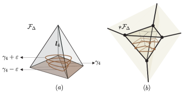
Figure 24: (a) Three loops $\gamma_{4}+\varepsilon$, $\gamma_{4}$, and $\gamma_{4}-\varepsilon$ in the primal lattice and (b) in the dual lattice.

We choose the loop such that it circles a point where these 3D hinges meet, say, point $p,$ which is the 2D hinge. In other words, our choice of loop will always cross these three hinges, so that the 3D hinges in neither ’outside’ nor ’inside’ the loop (or both outside and inside). This is the origin of the ambiguity arise in our construction.

To solve this, let us define other loops, which is $\gamma_{4}+\varepsilon$ and $\gamma_{4}-\varepsilon$ through a homotopy map, with $\varepsilon$ is small. See FIG. 24. The loop $\gamma+\varepsilon$ is non-contractible, since it circles the three 3D hinges, while the loop $\gamma_{4}-\varepsilon$ is contractible. It is clear that $\gamma_{4}+\varepsilon$ is the loop where $\left.\,{}^{3}\boldsymbol{F}\right|_{\Sigma}$ is located, while $\gamma_{4}-\varepsilon$ is the loop satisfying relation (34).

Both of these argument are equally correct and well-defined, so it force us to interpret that there exist a fundamental fuzziness, that is, an impossibility to obtain sharps variables simultaneously, in discrete geometry. In particular, it is impossible to obtain the 2D and 3D holonomy simultaneously; to obtain the sharp 2D holonomy, one need to place the loop on the 2D surface, that is, loop $\gamma_{4}$, and this will lead to ambiguity in the holonomy of the 3D curvature. Meanwhile, to obtain a sharp 3D holonomy, one need to move the loop sligthly outside the 2D surface, which is $\gamma_{4}+\varepsilon$. Both of these holonomy can not be placed together on a same loop.

We interpret this as a fundamental fuzziness or ’non-commutativity’, which occurs due to the discrete nature of the geometries. In the (asymptotical) continuum limit, where the hinges become infinitesimal, $\varepsilon\sim 0$, and the two loops will coincide, therefore, the non-commutativity trait between the 3D and 2D curvature will dissapear, which is reflected through the continuous Gauss-Codazzi equation.

Another fact which strengthen our argument about the existence of the fundamental fuzziness in discrete geometry is already explained in Subsection IV C, which is the impossibility in obtaining the discrete 2D intrinsic and extrinsic curvature simultaneously.

V.3 Recovering the Second Order Formulation

To obtain the second order formulation of gravity, one needs the triads $e$ coming from the local trivialization between the bundle and its standard. With the triads satisfying torsionless condition:

$$d_{D}e=0,$$

one could obtain the following relation:

$$e\left(\boldsymbol{F}\right)=\boldsymbol{R},$$

with $\boldsymbol{R}$ are the Riemann curvature tensor of the base manifold $M$.

The torsionless condition guarantees the Bianchi identity (35). With the torsionless triads, one could obtain the second order variables of general relativity. It must be kept in mind that the triads maps alter the coordinate of the plane or rotation, but not the angles relation, since the trace of holonomy is invariant under diffeomorphism. The torsionless condition also reduce the degrees of freedom in the 3-dimensional system, from nine components of $F_{\mu\nu J}^{I}$ to six components of $R_{\mu\nu\beta}^{\alpha}$.

But even in the second order formulation point of view, we still have a similar geometrical interpretation as explained in Subsection IV A, but with all geometrical quantities embedded in the base space $M.$ This is due to the fact that the loop orientation plane and the rotation bivector in general do not coincide. In fact, using a specific coordinate, one could write the Riemann tensor such that all the components are zero, except $R_{\nu\mu\nu}^{\mu}.$ This means there exist a coordinate where the two planes coincide. As a consequence, in discrete geometry, it is convenient to treat the loop orientation plane purely as a coordinate property, or a pure gauge. The use of the base space is cumbersome in discrete geometries, which may indicate that the base space is related to a dependent background structure.

V.4 Conclusions

We have clarified the definitions and the geometrical interpretation of curvatures, Bianchi identity, and Gauss-Codazzi equation in the first order Regge calculus setting. Our variables and relations converge to their continuous counterparts in the continuum limit. The case studied in this work is $\left(2+1\right)$-dimensional. A generalization to higher dimension of these results is possible and highly encouraged. In particular, it is interesting to see if it is possible to obtain a compactly written formula for a $\left(3+1\right)$-dimensional case. Furthermore, as a more ambitious goal, the trivalent condition could be geometrically interpreted as a spherical triangle, which could be use as a building blocks for higher dimensional spherical simplex.

References

- (1) C. Rovelli. Notes for a brief history of quantum gravity. Marcel Grossmann Meeting on Recent Developments in Theoretical and Experimental General Relativity. arXiv:gr-qc/0006061.
- (2) S. Carlip, D. Chiou, W. Ni, R. Woodard. Quantum Gravity: A Brief History of Ideas and Some Prospects. Int. J. Mod. Phys. D 24. No. 11 (2015). arXiv:gr-qc/1507.08194
- (3) R. Arnowitt, S. Deser, C. Misner. Dynamical Structure and Definition of Energy in General Relativity. Phys. Rev. 116 (5): 1322-1330. (1959).
- (4) R. Arnowitt, S. Deser, C. Misner. The Dynamics of General Relativity. Gen. Rel. Grav. 40 (9): 1997–2027. (2004). arXiv:gr-qc/0405109.
- (5) P. A. M. Dirac. Generalized Hamiltonian Dynamics. Proceedings of the Royal Society of London A 246 (1246): 326–332. (1958).
- (6) P. A. M. Dirac. The Theory of Gravitation in Hamiltonian Form. Proceedings of the Royal Society of London A 246 (1246): 333–343. (1958).
- (7) P. A. M. Dirac. Fixation of Coordinates in the Hamiltonian Theory of Gravitation. Phys. Rev. 114 (3): 924–930. (1959).
- (8) P. Bergmann. Hamilton–Jacobi and Schrodinger Theory in Theories with First-Class Hamiltonian Constraints. Phys. Rev. 144 (4): 1078–1080. (1966).
- (9) P. A. M. Dirac. The Fundamental Equations of Quantum Mechanics. Proceedings of the Royal Society A: Mathematical, Physical and Engineering Sciences 109 (752): 642. (1925).
- (10) P. A. M. Dirac. Lectures on Quantum Mechanics. Snowball Publishing. ISBN-13: 978-1607964322. (2012).
- (11) B. S. DeWitt. Quantum Theory of Gravity. I. The Canonical Theory. Phys. Rev. 160 (5): 1113–1148. (1967).
- (12) J. B. Hartle, S. W. Hawking. Wave function of the Universe. Phys. Rev. D 28: 2960–2975. (1983).
- (13) E. Cartan. Sur une généralisation de la notion de courbure de Riemann et les espaces á torsion. C. R. Acad. Sci. 174: 593-595. (1922).
- (14) A. Ashtekar. New Hamiltonian formulation for general relativity. Phys. Rev. D 36: 6. (1987). PRD36p1587_1987.pdf
- (15) A. Ashtekar. Lectures on non-perturbative canonical gravity. Bibliopolis. Naples. (1998).
- (16) S. Holst. S. Barbero’s Hamilitonian derived from a generalized Hilbert-Palatini action. Phys. Rev. D 53: 5966-5969. (1996).
- (17) G. Barbero. Real Ashtekar variables for Lorentzian signature space-times. Phys. Rev. D 51 (10): 5507-5510. (1995).
- (18) G. Immirzi. Real and complex connections for canonical gravity. Class. Quantum Grav. 14: L177-L181. (1997).
- (19) C. Rovelli, L. Smolin. Loop space representation of quantum general relativity. Nucl. Phys. B 331 (1): 80-152. (1990).
- (20) C. Rovelli, L. Smolin. Knot Theory and Quantum Gravity. Phys. Rev. Lett. 61 (10): 1155–1958. (1988).
- (21) C. Rovelli. Loop Quantum Gravity. Living Rev. Relativity 1. (1998). http://www.livingreviews.org/lrr-1998-1.
- (22) C. Rovelli. Quantum Gravity. Cambridge Monographs on Mathematical Physics. (2004).
- (23) T. Thiemann. Introduction to Modern Canonical Quantum General Relativity. (2001). arXiv:gr-qc/0110034.
- (24) C. Rovelli, L. Smolin. Discreteness of area and volume in quantum gravity. Nucl. Phys. B 442: 593–622. (1995). arXiv:gr-qc/9411005
- (25) A. Ashtekar, J. Lewandowski. Quantum theory of geometry. I: Area operators. Class. Quant. Grav. 14: A55–A82. (1997). arXiv:gr-qc/9602046.
- (26) A. Ashtekar, J. Lewandowski. Quantum theory of geometry. II: Volume operators. Adv. Theor. Math. Phys. 1: 388-429. (1998).arXiv:gr-qc/9711031.
- (27) H. Sahlmann, T. Thiemann, O. Winkler. Coherent states for canonical quantum general relativity and the infinite tensor product extension. Nucl. Phys. B 606: 401–440. (2001). arXiv:gr-qc/0102038.
- (28) B. Dittrich. The continuum limit of loop quantum gravity -a framework for solving the theory. (2014). arXiv:gr-qc/1409.1450.
- (29) B. Dittrich. From the discrete to the continuous - towards a cylindrically consistent dynamics. New Journal of Physics 14. (2012). arXiv:gr-qc/1205.6127.
- (30) C. Kiefer. The semiclassical approximation to quantum gravity. arXiv:gr-qc/9312015.
- (31) J. W. Barrett, T. J. Foxon. Semiclassical limits of simplicial quantum gravity. Class. Quant. Grav. 11 (3).arXiv:gr-qc/1409.1450
- (32) E. R. Livine. Some Remarks on the Semi-Classical Limit of Quantum Gravity. arXiv:gr-qc/0501076
- (33) T. Regge. General relativity without coordinates. Nuovo Cim. 19 (1961) 558. http://www.signalscience.net/files/Regge.pdf.
- (34) T. Regge, R. M. Williams. Discrete structures in gravity. J. Math. Phys. 41, 3964 (2000). arXiv:gr-qc/0012035v1.
- (35) J. W. Barrett and I. Naish-Guzman. The Ponzano-Regge model. Class. Quant. Grav. 26: 155014 (2009). arXiv:gr-qc/0803.3319.
- (36) J. W. Barrett. First order Regge calculus. Class. Quant. Grav. 11: 2723-2730. (1994). arXiv:hep-th/9404124.
- (37) H. Waelbroeck. 2+1 lattice gravity. Class. Quant. Grav. 7 (5). (1990). http://iopscience.iop.org/article/10.1088
- (38) G. t’Hooft. Causality in 2+1 Dimension. Class. Quant. Grav. 9 (5). (1992).
- (39) H. Waelbroeck, J. A. Zapata. A Hamiltonian lattice formulation of topological gravity. Class. Quant. Grav. 11 (4). (1994).
- (40) A. Ashtekar, V. Husain, C. Rovelli, J. Samuel, L. Smolin. 2+1 quantum gravity as a toy model for the 3+1 theory. Class. Quant. Grav. 6 (10). (1989).
- (41) V. Khatsymovsky. Regge calculus in the canonical form. Gen. Rel. Grav. 27: 583-603. (1995). arXiv:gr-qc/9310004
- (42) L. Brewin. The Gauss-Codacci equation on a Regge spacetime. Class. Quant. Grav. 5 (9). (1988).
- (43) L. Brewin. The Gauss-Codacci equation on a Regge spacetime II. Class. Quant. Grav. 10 (5). (1993).
- (44) P. A. Hoehn. Canonical linearized Regge Calculus: counting lattice gravitons with Pachner moves. Phys. Rev. D 91: 124034. (2015). arXiv:gr-qc/1411.5672.
- (45) S. Ariwahjoedi, J. S. Kosasih, C. Rovelli, F. P. Zen. Curvatures and discrete Gauss-Codazzi equation in (2+1)-dimensional loop quantum gravity. IJGMMP 12: 1550112. (2015). arXiv:gr-qc/1503.05943
- (46) L. Brewin. The Riemann and extrinsic curvature tensors in the Regge calculus. Class. Quant. Grav. 5 (9). (1988).
- (47) J. R. McDonald, W. A. Miller. A geometric construction of the Riemann scalar curvature in Regge calculus. Class. Quant. Grav. 25: 195017. (2008). arXiv:gr-qc/0805.2411
- (48) J. W. Barret. The geometry of classical Regge calculus. Class. Quant. Grav. 4 (6). (1987). http://cds.cern.ch/record/173023
- (49) B. Bahr, B. Dittrich. Regge calculus from a new angle. New J. Phys. 12: 033010. (2010). arXiv:gr-qc/0907.4325.
- (50) R. Conboye, W. A. Miller, S. Ray. Distributed mean curvature on a discrete manifold for Regge calculus. Class. Quantum Grav. 32: 185009. (2015). arXiv:math-dg/1502.07782
- (51) R. Conboye. Piecewise Flat Extrinsic Curvature. arXiv:math-dg/1612.07753
- (52) H. W. Hamber, G. Kagel. Exact Bianchi identity in Regge gravity. Class. Quantum Grav. 21: 5915–5947. (2004).
- (53) A. P. Gentle, A. Kheyfets, J. R. McDonald, W. A. Miller. A Kirchhoff-like conservation law in Regge calculus. Class. Quant. Grav. 26: 015005. (2009). arXiv:gr-qc/0807.3041
- (54) R. M. Williams. The contracted Bianchi identities in Regge calculus. Class. Quant. Grav. 29 (9). (2012).
- (55) F. Luo. Rigidity of Polyhedral Surfaces. (2006). arXiv:math-GT/0612714.
- (56) J. R. McDonald, W. A. Miller. A Discrete Representation of Einstein’s Geometric Theory of Gravitation: The Fundamental Role of Dual Tessellations in Regge Calculus. arXiv:gr-qc/0804.0279.
- (57) H. W. Hamber. Quantum Gravitation: The Feynman Path Integral Approach. Springer-Verlag. ISBN 978-3-540-85292-6. (2009).
- (58) H. W. Hamber. Quantum gravity on the lattice. Gen. Rel. Grav. 41: 817-876. (2019).
- (59) E. Gourgoulhon. 3+1 Formalism and Bases of Numerical Relativity. arXiv:gr-qc/0703035.
- (60) B. Dittrich, S. Speziale. Area-angle variables for general relativity. New. J. Phys. 10: 083006. (2008). arXiv:gr-qc/0802.0864.
- (61) B. Delaunay. Sur la sphere vide. Bulletin de l’Academie des Sciences de l’URSS, Classe des sciences mathematiques et naturelles 6: 793–800. (1934).
- (62) W. A. Miller. The Hilbert Action in Regge Calculus. Class. Quant. Grav. 14: L199-L204. (1997). arXiv:gr-qc/9708011
- (63) G. Calcagni, D. Oriti, J. Thurigen. Laplacians on discrete and quantum geometries. Class. Quantum Grav. 30: 125006. (2013) arXiv:gr-qc/1208.0354
- (64) J. A. Zapata. Topological lattice gravity using self-dual variables. Class. Quant. Grav. 13: 2617-2634. (1996). arXiv:gr-qc/9603030
- (65) J. A. Zapata. Combinatorial space from loop quantum gravity. Gen. Rel. Grav. 30: 1229-1245. (1998). arXiv:gr-qc/9703038
- (66) J. R. Munkres. Topology ( edition). Prentice Hall. ISBN 0-13-181629-2. (2000).
- (67) S. Ariwahjoedi, J. S. Kosasih, C. Rovelli, F. P. Zen. Degrees of freedom in discrete geometry. arXiv:gr-qc/1607.07963
- (68) H. M. Haggard, M. Han, A. Riello. Encoding Curved Tetrahedra in Face Holonomies: a Phase Space of Shapes from Group-Valued Moment Maps. Annales Henri Poincare 17 (8): 2001-2048. (2016). arXiv:math-ph/1506.03053.
- (69) A. E. Fekete. Real Linear Algebra. CRC Press. (1985).