Ferromagnetic Potts models with multi-site interaction

Abstract

We study the $q$ states Potts model with four site interaction on the square lattice. Based on the asymptotic behaviour of lattice animals, it is argued that when $q\leq 4$ the system exhibits a second-order phase transition, and when $q>4$ the transition is first order. The $q=4$ model is borderline. We find ${1}/{\ln q}$ to be an upper bound on $T_{c}$, the exact critical temperature. Using a low-temperature expansion, we show that $1/(\theta\ln q)$, where $\theta>1$ is a $q$-dependent geometrical term, is an improved upper bound on $T_{c}$. In fact, our findings support $T_{c}=1/(\theta\ln q)$. This expression is used to estimate the finite correlation length in first-order transition systems. These results can be extended to other lattices. Our theoretical predictions are confirmed numerically by an extensive study of the four-site interaction model using the Wang-Landau entropic sampling method for $q=3,4,5$. In particular, the $q=4$ model shows an ambiguous finite-size pseudocritical behaviour.

I Introduction

The Potts model Potts and Domb (1952); Wu (1982) has been widely explored in the literature for the last few decades. While many analytical and numerical results exist for the traditional two-site interaction model in various geometries and dimensions Wu (1982), little is yet known about models with multisite interactions Baxter et al. (1978); Enting and Wu (1982); Baxter et al. (1978); Wu (1979); Wu and Lin (1980); Wu and Zia (1981). Baxter $et~{}al.$ Baxter et al. (1978) and Wu $et~{}al.$ Wu (1979); Wu and Lin (1980); Wu and Zia (1981) obtained the exact transition point for the three-site interaction model on the triangular lattice. The four-spin interaction model has been studied by several authors Giri et al. (1977); Kunz and Wu (1978); Burkhardt (1979). Specifically, it has been shown Giri et al. (1977); Kunz and Wu (1978) that the site percolation problem on the square lattice can be formulated as a four site interaction Potts model in the limit $q\to 1$. Burkhardt Burkhardt (1979) argued that the four-site Hamiltonian $\cal H$, with interaction strength $K$ defined for every other square of the lattice (chequerboard), can be mapped onto another four-site Hamiltonian $\tilde{\cal H}$ with strength $\tilde{K}$, defined for every elementary square in the dual lattice. This mapping yielded the transformation

$$(e^{K}-1)(e^{\tilde{K}}-1)=q^{3},$$ (1)

in agreement with a more general expression Essam (1979); Wu (1982)

$$(e^{K_{\gamma}}-1)(e^{\tilde{K}_{\gamma}}-1)=q^{\gamma-1},$$ (2)

which assumes arbitrary $\gamma$ site interaction. Results like (1) and (2) may be conveniently obtained if one equivalently represents the Potts spin configurations as graphs on regular lattices Wu (1982); Baxter (1973a, b). However, the set of monochromatic graphs associated with non-zero interaction terms in the checkerboard Hamiltonian, is small compared to the set of monochromatic graphs involved in the partition sum of a problem where every elementary square is considered. Therefore, (1) suggests that the transition point (if it exists) should be rather different from that of a four site interaction model defined for every elementary square.

In this paper we consider a four site interaction model described by a Hamiltonian with a partition sum that exhausts all the elementary squares of the lattice. We propose a simple equilibrium argument that results in a critical condition for the transition point. This condition is in fact a zeroth-order approximation to the exact point. It relies on the observation that tracing out spin states in the partition sum is equivalent to the enumeration of large scale lattice animals at the vicinity of the transition point. Using a self consistent low temperature approximation, we obtain a more general condition which may allow one to approach the exact point up to an arbitrarily small distance by means of the first-order finite correlation length, at least when $q>4$. It is argued that these considerations can be applied to other lattices. To demonstrate the generalization, we briefly also discuss the triangular lattice. We next test our analytical predictions by an extensive numerical study of the four-site interaction Potts model on the square lattice (FPS) with $q=3,4,5$ states per spin. For that purpose we use the Wang-Landau (WL) Wang and Landau (2001a, b) entropic sampling method. The simulations results, together with finite size scaling (FSS) analysis, enable us to approximate the infinite lattice transition point for each of the three models. An estimate of the correlation length for the $q=5$ model, which according to the simulations exhibits a strong first-order transition, is additionally made. It should be noted that another microcanonical-ensemble-based approach that may be useful in simulating the first-order transition FPS has been introduced in Martin-Mayor (2007).

The rest of the paper is organized as follows. In Sec. II we present the model and describe the role of lattice animals in determining the order of the phase transition. We find the (seemingly) exact transition point and show it is related to the finite correlation length in the first-order transition case. In Sec. III we present the WL simulations results and FSS analysis. Our conclusions are drawn in Sec. IV.

II Analytical results

We consider the FPS, defined by the Hamiltonian

$$-\beta{\mathcal{H}}=K\sum_{\square}\delta_{\sigma_{\square}},$$ (3)

where $\beta=1/k_{B}T$ and $K=\beta J$ is the dimensionless coupling strength (for convenience we will assume from now on $k_{B}=J=1$). Each spin can take an integer value $1,2,...,q$. The $\delta_{\sigma_{\square}}$ symbol assigns $1$ if all the four spins in a unit cell $\square$ are equal and $0$ otherwise. The summation is taken over all the unit cells. It is convenient to write the partition function for the Hamiltonian (3) (Baxter, 2013)

$$Z_{N}=\sum_{\sigma_{\square}}\prod_{\square}(1+v\delta_{\sigma_{\square}})\sim q^{N}\sum_{G}q^{c(G)-\nu(G)}v^{f(G)},$$ (4)

where $v=e^{K}-1$ and $G$ is a graph made of $f(G)$ unit cell faces placed on the edges of the lattice. The faces are grouped into $c(G)$ clusters with a total number of $\nu(G)$ nodes. The $\sim$ sign is due to contributions to the partition sum from perimeter terms $o(N)$, which are omitted. Clusters with perimeters of size $O(N)$ (snakelike, snail-like, etc.) are energetically unfavourable and also assumed to be poor in entropy; therefore their corresponding graph contributions are absent. An illustration of a graph $G$ is given in Fig. 1. Provided all the interacting spins are shown in the figure, $G$ is associated with a $q^{N-39}v^{18}$ term in (4).

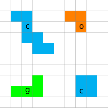
Figure 1: A portion of the square lattice showing a graph $G$ with $c(G)=4$ monochromatic clusters, $f(G)=18$ faces (coloured squares), and $\nu(G)=43$ nodes residing in the corners of these squares. The three different colours (also denoted by c,g,o) represent a model with $q\geq 3$.

We now consider a low temperature expansion ($v\approx u=e^{K}$) in which we assume only $k$ clusters exist. That is, for each $k$ large enough we assume a single cluster [$c(G)=1$] with $f(G)=k$ faces and $\nu(G)=m_{k}$ sites. It is conjectured that in a typical $k$ cluster $m_{k}\approx k$. In terms of the new variables, the low temperature partition function may take the form

$$Z_{N}^{\rm low}\propto q^{N}\sum_{k}\sum_{m_{k}}{\cal G}(k,m_{k})q^{-m_{k}}u^{k},$$ (5)

where ${\cal G}(k,m_{k})$ is the number of configurations with $k$ faces and $m_{k}$ sites, associated with a $k$ cluster. It is known Barequet et al. (2016); Klarner and Rivest (1973); Jensen (2003) that the combinatorial term $g_{k}=\sum_{m_{k}}{\cal G}(k,m_{k})$ for large $k$ is the asymptotic number of lattice animals $g_{k}\approx c\lambda^{k}/k$, where $\lambda\approx 4.0626$ and $c\approx 0.3169$. This observation distinguishes between $q>4$ and $q\leq 4$. Making a $k$ cluster (animal) monochromatic, the total change in entropy if an asymptotic number of site configurations is exhausted, can be written, to leading order, as

$$\Delta S_{\text{tot}}=k\ln(\lambda/q).$$ (6)

Thus, when $q>\lambda>4$, it is energetically disadvantageous for the system to occupy animals at the asymptotic rate. Instead, to optimize the energy gain to entropy loss ratio, it possesses a giant component (GC), typically at the system size, that may be distorted from a perfect square in shape. This mechanism is usually associated with systems which exhibit a first-order phase transition. In the case that $q\leq 4$, since $\lambda>q$, the entropy of the system increases. To avoid this, the system will again form a GC but this time with a fractal dimension rather than a simple component as in the $q>4$ case. This scenario is typical to second-order transitions, where the correlation length at criticality diverges. A single monochromatic GC approximately reduces the entropy in the amount of $\Delta S=-\ln q^{k_{GC}+h.o.t}\approx-\ln q^{k_{GC}}$. The resulting gain in energy is $\Delta E=-k_{GC}$. Thus, $\Delta F=\Delta E-T\Delta S<0$ if and only if $T<1/\ln q$, yielding the zeroth-order bound on the critical point

$$\tilde{T}_{c}=\frac{1}{\ln q}.$$ (7)

Consider for a first-order $q$ the class (denoted by $\hat{A}$) of large $k$ animals with perimeters proportional (to leading order) to $\sqrt{N}$. Higher order contributions to (6) from the simple GC may then be depicted by writing

$$\theta=\sup_{k}\left(\sup_{m_{k}}\frac{m_{k}}{k}\right),$$ (8)

where $m_{k}$ are now site variables of animals in $\hat{A}$. Replacing $q^{-m_{k}}$ in (5) with $q^{-\theta k}$, it can be shown (see Appendix A) that

$$\Lambda=\lim_{N\to\infty}(Z_{N}^{\rm low})^{1/N}=uq^{1-\theta}.$$ (9)

The (minus) dimensionless free energy $-\beta f^{\rm low}=\ln\Lambda$ is then maximal if and only if $uq^{-\theta}>1$, leading to the critical condition

$$u_{c}=q^{\theta},$$ (10)

or equivalently to the critical temperature

$$\hat{T}_{c}=\frac{1}{\theta\ln q}.$$ (11)

Note that if one does not adopt the low temperature approximation, one has to add the term $\ln(1-1/u)$ to $-\beta f^{\rm low}$, hence does not violate the critical condition (10). Note also that long range order is uniquely controlled by large animals. These two observations imply that the critical temperature (11) is exact. Observe also the approximation $m_{k}=k$ (in the exponent) in (5) results in the critical condition $u_{c}=q$ and likewise (7). Equation (11) can be used to relate the critical point to the finite correlation length through

$$\theta=1+c_{1}/\xi+...,$$ (12)

where $\xi$ is a typical length for clusters that are not $k$ clusters. For instance, for the square lattice, it can be easily shown that the simple GC consists of $k$ faces and $m_{k}$ sites satisfying

$$\frac{m_{k}}{k}\leq 1+\frac{\hat{c}}{\sqrt{k}}+...$$ (13)

with $\hat{c}\geq 2$ constant. It follows from (12),(13) (see Appendix B) that $c_{1}=\hat{c}$. With the further aid of (11), one readily obtains

$$\hat{T}_{c}(q,\xi)=\frac{1}{\ln q}\left(1-\frac{\hat{c}}{\xi}\right)+O(1/\xi^{2}).$$ (14)

Finally, we address the issue of the lattice structure. In agreement with ref. Delfino and Tartaglia (2017), the formation mechanism of a GC, either simple or fractal, which controls the critical properties of the model, applies also to other systems. Specifically, the zeroth-order approximation (7) is expected to be valid (up to a constant multiplicative factor) for other lattices. In the first- order transition case, the lattice structure is captured by means of the constant term in  (14). For example, in the triangular lattice, a simple GC consisting of $m_{k}=k/2+O(\sqrt{k})$ sites, satisfies (14) with $\hat{c}\geq 1$. The lower bound corresponds to the marginal case where the GC, when embedded in the square lattice, forms a perfect monochromatic square with no vacancies.

III Simulations

To test our analytical predictions, we study the FPS for three different models, namely, with $q=3,4$ and $q=5$ states per spin. The Wang-Landau (WL) Wang and Landau (2001a, b) entropic sampling method is chosen for this purpose since it enables one to accurately compute canonical averages at any desired temperature. We use lattices with linear size $L=4,8,12,...,68$ and periodic boundary conditions are imposed. For each lattice size, we compute $\Omega(E)$, the number of states with energy $E$. These quantities allow us to calculate energy-dependent moments $\langle E^{n}\rangle\propto\sum_{E}E^{n}\Omega(E)e^{-\beta E}$. In particular, we are interested in the specific heat per spin given by Newman and Barkema (1999); Stanley (1987)

$$c_{L}=L^{-d}\beta^{2}(\langle E^{2}\rangle-\langle E\rangle^{2}).$$ (15)

A plot of the specific heat for the three models is given in Fig. 2. For each model, the location of the peak serves as $L$-dependent pseudo-critical temperature and is defined as $T_{L}\equiv T_{C_{L}^{\rm max}}$. Indeed, in agreement with (11), the pseudo-critical temperatures increase with $q$.

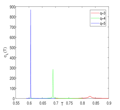
Figure 2: Variation of the specific heat of each model against temperature for $L=44$. While the $q=4$ model and especially the $q=5$ model display sharp and narrow peaks at the $q$-dependent position of the specific-heat maximum $T_{L}(q)$, the $q=3$ peak is an order of magnitude smaller and rather broad.

To determine the order of the transition for each model we are simultaneously also interested in the energy probability density. The latter may be written

$$P_{L}(\epsilon)\propto g_{L}(\epsilon)e^{-\beta L^{d}\epsilon}\approx L^{d}\Omega(E)e^{-\beta E},$$ (16)

with $\epsilon=L^{-d}E$ and $g_{L}(\epsilon)$ is the energy density of states. In Fig.  3a we display the probability density at $T_{L}(q)$. The $q=3,4$ models apparently suffer from significant finite-size effects. Specifically, the $q=4$ model has a double-peaked shape, usually seen in first-order transitions Janke (1993). Evidently, there is a large dip between the peaks, but (unlike in the $q=5$ case) also a domain where the two humps overlap. A fit of the minimal density between the peaks to a power law, generates a slope $-1.09\pm 0.19$. This may indicate finite-size interface contributions to the PDF. Either way, the dip does not exponentially vanish as expected from systems which undergo a discontinuous transition. When $q=5$, the energy is narrowly distributed in the vicinity of the ordered and disordered states’ energies (denoted by $\epsilon_{-}$ and $\epsilon_{+}$ respectively), and has a typical width $1/L$.

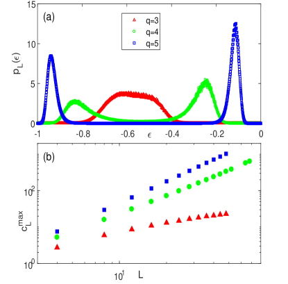
Figure 3: (a) Pseudo-critical canonical energy distribution computed at $T_{L}(q)$ for $q=3,4,5$ and $L=44$. Note the peaks width $1/L$ behaviour when $q=5$, typical to normal distributions. Conversely, the distributions for the $q=4$ (and of course the $q=3$) models are essentially not normal. (b) Scaling of the specific heat maximum $c_{L}^{\max}(q)$ with $L$ on a log-log scale for $q=3$ (${\color[rgb]{1,0,0}\blacktriangle}$), $q=4$ (${\color[rgb]{0,1,0}\bullet}$) and $q=5$ (${\color[rgb]{0,0,1}\blacksquare}$).

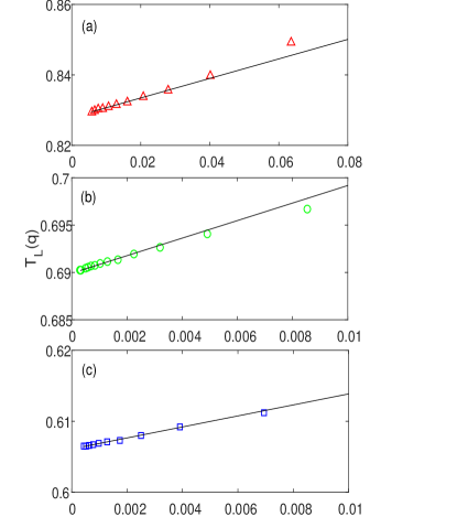
Figure 4: Scaling of the position [temperature $T_{L}(q)$] of the specific heat maximum with $L$, for the three models: (a) $q=3$ and $T_{L}-T_{c}\propto L^{-1/\nu}(\ln L)^{\alpha/\nu}$. (b) $q=4$ and $T_{L}-T_{c}\propto L^{-1/\nu+\text{h.o.t}}$. (c) $q=5$ and $T_{L}-T_{c}\propto L^{-d}$. Solid lines are presented to guide the eye.

Armed with these= observations we next perform a FSS analysis to each of the models. For each $q$ we locate $c_{L}^{\max}(q)$ and $T_{L}(q)$. We fit these observables to linear models according to conventional scaling laws. We then vary $L_{\min}$, the smallest lattice size used in the fit, simultaneously, and consider the intercept term in the $T_{L}(q)$ fit and the deviations of $T_{L}(q)$ ($L=L_{\min},...$) from the intercept, in a $\chi^{2}$ test Herdan (1955); Evans (1982). The best fit is determined for $L_{\min}>4$ from which the $p$ value becomes monotonically increasing. The corresponding $L_{\min}$ is denoted by $L_{\min}^{\text{best}}$. Since it is assumed [and evidently from Figs. 3b and 4 correct] that the exponents involved in the scaling laws of $c_{L}^{\max}(q)$ and $T_{L}(q)$ are not independent, it is reasonable that $L_{\min}^{\text{best}}$ simultaneously serves for the best fit of $c_{L}^{\max}(q)$. As observed in Fig. 3b, for $q=3$ it is plausible to try the ansatz $c_{L}^{\max}\approx(\ln L)^{\alpha/\nu}$ for the specific heat maximum. For the distance between $T_{L}$ and the infinite volume critical point, we use $T_{L}-T_{c}\propto L^{-1/\nu}(\ln L)^{\alpha/\nu}$ Kenna et al. (2006) and assume $\alpha,\nu$ satisfy the hyperscaling relation

$$d\nu=2-\alpha.$$ (17)

The goodness-of-fit test yields $\chi^{2}/\text{d.o.f}=1.14/7$, a $p$ value of 0.021 and $L_{\min}^{\text{best}}=20$ [from now on we will give for each $T_{L}(q)$ fit its corresponding $\chi^{2}/\text{d.o.f}$, followed by the $p$ value and $L_{\min}^{\text{best}}$, in parenthesis]. The intercept term in the $T_{L}(3)$ fit [Fig. 4a] is $0.827(9)$ and $\alpha/\nu\approx 2.197(5)$. The $q=4$ model displays a pronounced power-law scaling. Assuming a second order scaling law $c_{L}^{\rm max}\propto L^{\alpha/\nu}(1+AL^{-\omega}+o(L^{-\omega}))$, we focus on a correction to the leading order term. The distance between $T_{L}(4)$ and $T_{c}$ scales (to leading order) as $L^{-1/\nu}$. Again, next-to-leading-order unknown correction terms apparently involved. A fit to a power-law decay of $L$ yields an intercept term $0.689(9)$ ($1.72/7,0.044,32$). The specific heat maximum scales as $L^{1.832(7)}$. The picture is different when $q=5$. The rather asymptotic behaviour of the energy PDF as shown in Fig. 3a suggests the $q=5$ data are compatible with the first-order transition volume dependent scaling laws. The conventional $T_{L}-T_{c}\propto L^{-d}$ fit gives $T_{c}(5)\approx 0.606(1)$ ($2.08/8,0.033,16$). A log-log fit to $c_{L}^{\max}$ against $L$, for $L\geq 16$ gives a slope $1.992(6)$, so a volume-dependent scaling for the specific heat maximum is indeed conceivable. To further support a second-order behaviour when $q=4$ we consider the universal scaling form

$$c_{L}=L^{\alpha/\nu}{\cal F}(tL^{1/\nu}),$$ (18)

where ${\cal F}(x)$ is a universal scaling function of the dimensionless variable $x=tL^{1/\nu}$ and $t=(T-T_{c})/T_{c}$ is the reduced temperature. As clearly shown in Fig. 5, the specific heat, normalized by $L^{\alpha/\nu}$, collapses on a single curve as follows from (18). Thus, it is reasonable to assume the hyperscaling relation indeed holds, in consistency with the scaling relations we use.

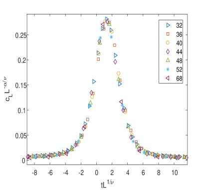
Figure 5: The specific heat universal scaling function ${\cal F}(x)$ for several lattice sizes $L$. The estimated values $T_{c}(4)\approx 0.689(9)$ and $\alpha/\nu\approx 1.832(7)$ are used in all the plots.

Another manifestation of the $q=5$ discontinuous transition is the latent heat, estimated in two different ways. First, by measuring the distance between the locations of the peaks in a Gaussian fit to the energy PDF (Fig. 6) and then trying the ansatz $\Delta\epsilon_{L}^{\rm PDF}\approx\Delta\epsilon^{\rm PDF}_{\infty}+\text{const}\times L^{-d}$, and second, using Challa et al. (1986)

$$c_{L}^{\max}\approx\frac{(\epsilon_{+}-\epsilon_{-})^{2}}{4T_{c}^{2}}L^{d}+\frac{c_{+}+c_{-}}{2},$$ (19)

where $c_{+},c_{-}$ are temperature independent terms.

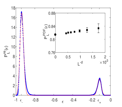
Figure 6: Reweighted PDF Janke (1993) (blue symbols) together with a double Gaussian fit for $L=44$. Note that the peaks are centred at points satisfying $P_{L}(\epsilon_{-})\approx qP_{L}(\epsilon_{+})$. The inset shows the difference between these points, as a function of $L^{-d}$ (closed squares). Absent error bars are smaller than the symbols. The estimated infinite volume $\Delta\epsilon_{\infty}^{\rm PDF}\approx 0.813(9)$ is denoted by the closed circle. Lattices with $L<24$ have too noisy distributions around the peaks and are therefore omitted.

The PDF fit, for $L\geq 24$, produces $\Delta\epsilon^{\rm PDF}_{\infty}=\epsilon_{+}^{\rm PDF}-\epsilon_{-}^{\rm PDF}\approx 0.813(9)$ ($\chi^{2}/\text{d.o.f}=1.35/6,p=0.058$) while (19), choosing $T_{c}(5)\approx 0.606(1)$, yields $\Delta\epsilon=\epsilon_{+}-\epsilon_{-}\approx 0.809(5)$. The two results reasonably agree.

To conclude, we turn to test our analytical predictions against some of the simulations results. First we compare the zeroth-order bounds with the simulations predictions. The results are summarized in Table 1. As expected, (7) becomes a better approximation as $q$ grows. Next, having in mind that for $q=5$ the transition is first order, we give a lower bound on the correlation length $\xi(5)$ with the help of (13) and (14). Taking $\hat{T}_{c}\approx 0.606(1)$ we obtain $\xi(5)>81$. This result justifies our FSS analysis in the sense that the lattice sizes we use are compatible with $\xi(5)$.

Table 1: Estimates of the transition temperatures for the three models, using the zeroth-order bound (7) and the simulations results. The relative error is given in the last column. The supplementary $q=10$ result is based on additional simulations for lattices with $4\leq L\leq 36$ and a $T_{L}-T_{c}\propto L^{-d}$ fit ($2.75/7,0.084,8$).

$q$	Bound	Simulations	Error (%)
3	0.910(2)	0.827(9)	9.9
4	0.721(3)	0.689(9)	4.6
5	0.621(3)	0.606(1)	2.5
10	0.434(2)	0.432(4)	0.4

IV conclusions

The transition nature of the FPS is controlled by large scale lattice animals. Based on the lattice animals asymptotic growth, the transition is found continuous for $q\leq 4$ and discontinuous for $q>4$. The $q=4$ is borderline. In the case in which the assumption that typical large clusters have (to leading order) the same number of sites and faces breaks down (e.g., when the number of clusters satisfying $\lim_{k\to\infty}\frac{m_{k}}{k}>1$ is sufficiently large), the $q=4$ model might undergo a first-order transition. It is expected that large animals growth controls the transition order in other lattices as well. Specifically, it is known Barequet et al. (2017) that the asymptotic number of triangular animals (polyamonds) of size $k$, $a_{k}$, satisfies $\lim_{k\to\infty}\sqrt[k]{a}_{k}=\lambda_{t}$ with $2.8424<\lambda_{t}<3.6050$. The number of faces in a typical large cluster is (to leading order) twice the number of sites. Thus, the transition is continuous $\it at~{}least$ for $q\leq 4$. Moreover, it can be easily shown the transition point is no larger than $2/\ln q$. The WL simulations and FSS analysis confirm our analytical predictions. That is, the $q=3$ model displays a scaling behaviour typical to a second-order transition and the $q=5$ numerical footprints are significantly first order. While the $q=3$ FSS shows a very slow approach to the asymptotic regime, the $q=5$ sample sizes are compatible with $\xi(5)$. The $\chi^{2}$ goodness-of-fit tests support the scaling laws we use. In particular, for $q=3$ it follows that the free-energy is homogeneous in the small-$L$ regime, since the critical indices apparently obey (up to small corrections) (17). The $q=4$ model is rather unique. The double-peaked shape of the energy distribution is also observed in models exhibiting a relatively weak first-order transition such as the $q=8$ usual Potts model, [see Fig. 1c in Janke (1993)]. On the other hand, Fig. 5 remarkably confirms (18), suggesting a divergence of the correlation length $\xi(4)\propto|t|^{-\nu}$ as $t\to 0$. The indefiniteness of the four-state model manifested both analytically and numerically, is in agreement with renormaliztion group (RG) predictions. The dynamics of models lying in the universality class of the two-site interaction $q=4$ Potts model (TSP) flows towards the multicritical point $q_{c}=4$ Nienhuis et al. (1979); Nauenberg and Scalapino (1980); Cardy et al. (1980). However, a certain choice of parameters Blöte et al. (2017) may drive the dynamics in some of these models away from $q_{c}$, to the first-order domain. In other words, in the marginal $q=4$ case, the transition nature (first versus second order) is sensitive to the model’s details Blöte et al. (2017). The lattice animals mechanism suggests that FPS may belong to the TSP universality class. Nevertheless, it leaves room for a first-order-like RG description. It should be emphasized that unlike the RG method which makes assumptions on the model under scaling, our approach is direct and fundamental, building on first principles, and thus, we think, is preferable to RG for the studied question. As a concluding remark, we believe that being general, our theoretical framework can be extended to other lattices, more complicated Hamiltonians and higher dimensions.

Appendix A The critical point

A.1 Derivation of equation (9)

We give a detailed derivation of (9) yielding the critical temperature (11). Since (11) is also useful in estimating the finite correlation length in the first-order case [see. (12) and Appendix B], the derivation concerns with this class of models. However, it is stressed that (11) holds for arbitrary $q$.

Let $\epsilon_{n}$ be a sequence of positive small numbers. Then there exist a sequence $k(\epsilon_{n})$ and sets

$$\kappa_{n}=\left\{~{}k>k(\epsilon_{n})~{}:~{}\left|\frac{\sum_{m_{k}}{\cal G}(k,m_{k})}{c\lambda^{k}/k}-1\right|<\epsilon_{n}\right\},$$ (20)

associated with animals ${\cal G}(k,m_{k})$ with $k$ faces and $m_{k}$ sites in the asymptotic regime. Consider further, for every $n$, the set $A_{n}$ of all the animals with an asymptotic $k$

$$A_{n}=\left\{~{}{\cal G}(k,m_{k})~{}:~{}k\in\kappa_{n}\right\}.$$ (21)

We now define the (small) class of large-$k$ simple animals

$$\hat{A}=\left\{{\cal G}(k,m_{k})\in\bigcup_{n}A_{n}~{}:~{}\frac{m_{k}-k}{\sqrt{k}}\leq B\right\},$$ (22)

where $B$ is a positive constant. Equations (20)-(22) allow us to define

$$\theta=\sup_{k}\left(\sup_{m_{k}:~{}{\cal G}(k,m_{k})\in\hat{A}}\frac{m_{k}}{k}\right).$$ (23)

Next, let $r_{j},~{}j=1,2,...,j_{\max}\leq{\cal N},~{}{\cal N}\in\bigcup_{n}\kappa_{n}$ be a sequence satisfying $\frac{1}{{\cal N}}<r_{j}<\frac{2}{{\cal N}}$. Construct another sequence with $j_{\max}$ integers $k_{j}\leq{\cal N}$ from $\bigcup_{n}\kappa_{n}$. Define now for every $1\leq j\leq j_{\max}$

$$\hat{A_{j}}=\left\{{\cal G}(k_{j},m_{k_{j}})\in\hat{A}~{}\text{s.t}~{}\frac{m_{k_{j}}}{k_{j}}>\theta-r_{j}\right\}.$$ (24)

Take $Z_{N}^{\rm low}\leq\hat{Z}_{{\cal N}}^{\rm low}$ where

$$\hat{Z}_{{\cal N}}^{\rm low}\propto q^{{\cal N}}\sum_{j}\sum_{m_{k_{j}}}{\cal G}(k_{j},m_{k_{j}})q^{-m_{k_{j}}}u^{k_{j}}$$

$$\leq q^{{\cal N}}\sum_{j}\sum_{m_{k_{j}}}{\cal G}(k_{j},m_{k_{j}})\left(\frac{u}{q^{\theta-r_{j}}}\right)^{k_{j}}$$

$$\leq q^{{\cal N}}\sum_{j}\hat{g}_{k_{j}}\left(\frac{u}{q^{\theta-2/{{\cal N}}}}\right)^{k_{j}}$$

$$\leq q^{{\cal N}}\left[K{\cal N}\binom{{\cal N}}{a\sqrt{{\cal N}}}\left(\frac{u}{q^{\theta-2/{{\cal N}}}}\right)^{{\cal N}}+o(\lambda^{\cal N})\right].$$ (25)

The $m_{k_{j}}$ summations in (A.1) taken over site variables of animals in $\hat{A_{j}}$, satisfy

$$\sum_{m_{k_{j}}}{\cal G}(k_{j},m_{k_{j}})\leq\hat{g}_{k_{j}}.$$ (26)

Since $\hat{g}_{k_{j}}$ count simple animals, their contributions to the leading order term are no larger than $K\binom{{\cal N}}{a\sqrt{{\cal N}}}$ where $K,a$ are constants. It follows immediately from (A.1) that

$$\lim_{{\cal N}\to\infty}(\hat{Z}_{{\cal N}}^{\rm low})^{1/{{\cal N}}}=\lim_{N\to\infty}(Z_{N}^{\rm low})^{1/N}=uq^{1-\theta}.$$ (27)

A.2 Equation (8) and first-order transitions

When the system undergoes a first-order phase transition, $q$ ordered states coexist with a single disordered state at the critical point. In (8) we utilize this as follows. Consider a simple large animal with $k=\alpha N~{}(\alpha<1)$ faces and $m_{k}$ sites. Then, the change in the free energy when making a macroscopic number of finite clusters monochromatic may be written

$$\Delta F(k,m_{k},T)=N[-(1-\alpha)+\sigma(1-\alpha)$$

$$+(1-\alpha\text{\footnotesize$\frac{m_{k}}{k}$})T\ln q]+\text{h.o.t},$$ (28)

where $0<\sigma<1$ controls the energy loss due to boundary interactions of the finite clusters. Applying now (23) to (A.2) gives $\Delta F_{u}(T)\leq\Delta F(k,m_{k},T)$ with

$$\Delta F_{u}(T)=N[-(1-\alpha)(1-\sigma)$$

$$+(1-\alpha\theta)T\ln q]+\text{h.o.t}.$$ (29)

Equation (A.2) holds provided the leading order term vanishes at the critical point. In addition, (A.2) should be unstable in some left neighbourhood of $T_{c}$. These can be established first by taking $\Delta F_{u}(T_{c})=\text{h.o.t}$ for $T_{c}=\hat{T}_{c}=1/(\theta\ln q)$, leading to

$$\theta=\frac{1}{1-\sigma(1-\alpha)}.$$ (30)

Second, consider $\Delta F_{s}(T)$, the free energy change due to the formation of a single giant component, given by

$$\Delta F_{s}(T)=N(-\alpha+\alpha\theta T\ln q)+\text{h.o.t}.$$ (31)

Plugging (30) into (A.2) and (31) it follows that $\Delta F_{s}(T_{c}^{-})<\Delta F_{u}(T_{c}^{-})$ if and only if

$$\alpha>\frac{1}{2\theta}.$$ (32)

Equations (A.2)-(32) assert that when a (first-order) phase transition occurs, the fraction of faces constructing a monochromatic GC is no smaller than $1/2\theta$. It should be noted that the critical threshold $\alpha_{c}=1/2\theta$ increases with $q$ (see Appendix B) in accordance with the system’s attempt to reduce entropy.

We conclude by stating that (9) [and so (11)] holds for the second-order models as well In order that the number of animals with $k$ faces to be maximal, the system picks those with a maximal number of sites. Equation (8) then immediately follows. In addition, constructing $\theta$, fractal animal are involved so that $\hat{A}$ in (23) may be replaced with ${\cal\hat{A}}\subseteq\bigcup_{n}A_{n}$ .

Appendix B The correlation length

In the following, we derive the relation between the first-order model finite correlation length and the critical temperature, formulated by (12). Observe that for animals in $\hat{A}$, (22) implies

$$\frac{m_{k}}{k}\leq 1+\frac{\hat{c}}{\sqrt{k}}+...$$ (33)

Hence there exist a sequence $\hat{k}_{n}\leq k(\epsilon_{n})$ such that

$$\theta\leq 1+\frac{\hat{c}}{\sqrt{\hat{k}_{n}}}+...,$$ (34)

leading to

$$\theta=1+\frac{c_{1}}{\xi}+...=\inf_{n}\left(1+\frac{\hat{c}}{\sqrt{\hat{k}_{n}}}+...\right),$$ (35)

with $[\xi^{2}]=\max_{n}(\hat{k}_{n})$ and $c_{1}=\hat{c}$. The correlation length, as follows from (35), may be interpreted as a typical length measuring large finite domains. Writing the RHS of (12) as a power series $\sum_{n=0}^{\infty}c_{n}x^{n}$ at $x=\xi^{-1}$, it follows from (30) that $\lim_{n\to\infty}\sqrt[n]{c_{n}}=\xi\sigma(1-\alpha)$ so the series indeed converges to $\theta$.

Observe that the above analysis can be extended to arbitrary $q$ first-order systems. We expect that as $q$ grows the deviations from a perfect square critical giant component become smaller. This may be formulated by constructing subclasses $\hat{A}(q)\subseteq\hat{A}$ with animals ${\cal G}(k,m_{k})$ satisfying $\sup_{k}\frac{m_{k}-k}{\sqrt{k}}=B(q)$, where the constants $B(q)$ are expected to decrease with $q$. Replacing $\hat{A}$ in (23) with $\hat{A}(q)$, $\theta$ essentially becomes $q$ dependent. It acquires lower values as $q$ grows, as also realized in Table 1, where the simulated temperature approaches better the bound $1/\ln q$, when $q$ changes from $q=5$ to $q=10$.

References

- Potts and Domb (1952) R. B. Potts and C. Domb, Mathematical Proceedings of the Cambridge Philosophical Society 48, 106 (1952).
- Wu (1982) F. Y. Wu, Reviews of Modern Physics 54, 235 (1982).
- Baxter et al. (1978) R. J. Baxter, H. N. V. Temperley, and S. E. Ashley, Proceedings of the Royal Society A: Mathematical, Physical and Engineering Sciences 358, 535 (1978).
- Enting and Wu (1982) I. G. Enting and F. Y. Wu, Journal of Statistical Physics 28, 351 (1982).
- Wu (1979) F. Y. Wu, Journal of Physics C: Solid State Physics 12, L645 (1979).
- Wu and Lin (1980) F. Y. Wu and K. Y. Lin, Journal of Physics A: Mathematical and General 13, 629 (1980).
- Wu and Zia (1981) F. Y. Wu and R. K. P. Zia, Journal of Physics A: Mathematical and General 14, 721 (1981).
- Giri et al. (1977) M. R. Giri, M. J. Stephen, and G. S. Grest, Physical Review B 16, 4971 (1977).
- Kunz and Wu (1978) H. Kunz and F. Y. Wu, Journal of Physics C: Solid State Physics 11, L357 (1978).
- Burkhardt (1979) T. W. Burkhardt, Physical Review B 20, 2905 (1979).
- Essam (1979) J. W. Essam, Journal of Mathematical Physics 20, 1769 (1979).
- Baxter (1973a) R. J. Baxter, Journal of Physics C: Solid State Physics 6, L445 (1973a).
- Baxter (1973b) R. J. Baxter, Journal of Statistical Physics 9, 145 (1973b).
- Wang and Landau (2001a) F. Wang and D. P. Landau, Physical Review Letters 86, 2050 (2001a).
- Wang and Landau (2001b) F. Wang and D. P. Landau, Physical Review E 64, 6101 (2001b).
- Martin-Mayor (2007) V. Martin-Mayor, Physical Review Letters 98, 7207 (2007).
- Baxter (2013) R. J. Baxter, Exactly Solved Models in Statistical Mechanics (Dover Books on Physics) (Dover Publications, 2013).
- Barequet et al. (2016) G. Barequet, G. Rote, and M. Shalah, Communications of the ACM 59, 88 (2016).
- Klarner and Rivest (1973) D. A. Klarner and R. L. Rivest, Journal canadien de mathématiques 25, 585 (1973).
- Jensen (2003) I. Jensen, in Lecture Notes in Computer Science (Springer Berlin Heidelberg, 2003) pp. 203–212.
- Note (1) It can be shown that clusters and clusters of size do not share mutual ”corner” sites, asymptotically almost surely.
- Delfino and Tartaglia (2017) G. Delfino and E. Tartaglia, Physical Review E 96, 2137 (2017).
- Newman and Barkema (1999) M. E. J. Newman and G. T. Barkema, Monte Carlo Methods in Statistical Physics (Clarendon Press, 1999).
- Stanley (1987) H. E. Stanley, Introduction to Phase Transitions and Critical Phenomena (International Series of Monographs on Physics) (Oxford University Press, 1987).
- Janke (1993) W. Janke, Physical Review B 47, 14757 (1993).
- Herdan (1955) G. Herdan, Journal of Polymer Science 17, 315 (1955).
- Evans (1982) R. D. Evans, Atomic Nucleus (Krieger Pub Co, 1982).
- Kenna et al. (2006) R. Kenna, D. A. Johnston, and W. Janke, Physical Review Letters 96, 5701 (2006).
- Challa et al. (1986) M. S. S. Challa, D. P. Landau, and K. Binder, Physical Review B 34, 1841 (1986).
- Barequet et al. (2017) G. Barequet, M. Shalah, and Y. Zheng, in Lecture Notes in Computer Science (Springer International Publishing, 2017) pp. 50–61.
- Nienhuis et al. (1979) B. Nienhuis, A. N. Berker, E. K. Riedel, and M. Schick, Physical Review Letters 43, 737 (1979).
- Nauenberg and Scalapino (1980) M. Nauenberg and D. J. Scalapino, Physical Review Letters 44, 837 (1980).
- Cardy et al. (1980) J. L. Cardy, M. Nauenberg, and D. J. Scalapino, Physical Review B 22, 2560 (1980).
- Blöte et al. (2017) H. W. J. Blöte, W. Guo, and M. P. Nightingale, Journal of Physics A: Mathematical and Theoretical 50, 4001 (2017).
- Note (2) We take to make sure the inner supremum in (23) exists.