Non-iterative triples excitations in equation-of-motion coupled-cluster theory for electron attachment with applications to bound and temporary anions

Abstract

The impact of residual electron correlation beyond the equation-of-motion coupled-cluster singles and doubles approximation (EOM-CCSD) on positions and widths of electronic resonances is investigated. To establish a method that accomplishes this task in an economical manner, several approaches proposed for the approximate treatment of triples excitations are reviewed with respect to their performance in the electron attachment (EA) variant of EOM-CC theory.

The recently introduced EOM-CCSD(T)(a)* method, which includes non-iterative corrections to the reference and the target states, reliably reproduces vertical attachment energies from EOM-EA-CC calculations with singles, doubles, and full triples excitations in contrast to schemes in which non-iterative corrections are applied only to the target states.

Applications of EOM-EA-CCSD(T)(a)* augmented by a complex absorbing potential (CAP) to several temporary anions illustrate that shape resonances are well described by EOM-EA-CCSD, but that residual electron correlation often makes a non-negligible impact on their positions and widths. The positions of Feshbach resonances, on the other hand, are significantly improved when going from CAP-EOM-EA-CCSD to CAP-EOM-EA-CCSD(T)(a)*, but the correct energetic order of the relevant electronic states is still not achieved.

I Introduction

Quantum chemistry of bound electronic states has reached a level where quantitative agreement between theory and experiment is possible for many observables.elstbook The same has so far not been achieved for processes involving electronic resonances,jagau17 i.e., autoionizing states with finite lifetime embedded in the continuum. Although theoretical methods for resonances possess considerable predictive power,jagau17 sizable discrepancies between theory and experiment often still exist. Sources of uncertainty on the side of theory are manifold and can include errors introduced by improper handling of the resonance character, neglect of structural relaxation and vibrational effects, insufficient basis-set convergence, and incomplete treatment of electron correlation.

The latter issue motivates this article. While the general importance of electron correlation for resonances is well established,jagau17 ; sommerfeld98 ; white17 a quantification of higher-order correlation effects as routinely possible for bound states, has never been done for resonances. This is because their theoretical treatment is more demanding than that of bound states. Electronic resonances do not represent discrete $L^{2}$ integrable states in Hermitian quantum mechanics and only in a non-Hermitian formalism is it possible to treat them as discrete states with complex energy.nhqmbook ; jagau17 Strategies to compute complex resonance energies with bound-state electronic-structure methods include stabilization methods,hazi70 ; nestmann85 , analytic continuation of the coupling constant,horacek10 and especially complex-variable techniques such as complex scaling,aguilar71 ; balslev71 ; simon79 ; moiseyev79 , complex basis functions, mccurdy78 and complex absorbing potentials (CAPs).jolicard85 ; riss93 Particular advantages of the latter approach are its compatibility with the Born-Oppenheimer approximation and the possibility to extend techniques for computing molecular properties jagau16 and analytic energy gradients benda17 to electronic resonances.

When aiming at a high-accuracy treatment of electronic resonances in polyatomic molecules, the combination of complex-variable techniques with equation-of-motion coupled-cluster (EOM-CC) theory offers several formal advantages and is also numerically promising.ghosh12 ; bravaya13 ; zuev14 ; jagau16b ; white17 The EOM-CC formalism emrich80 ; geertsen89 ; stanton93 ; ccbook ; krylov08 ; sneskov12 allows to treat electronically excited stanton93 (EOM-EE), ionized stanton94 (EOM-IP), and electron-attached nooijen95 (EOM-EA) states as eigenfunctions of the same effective Hamiltonian, which is crucial for electronic resonances because it enables a consistent description of a resonance relative to the ionization and detachment continua.jagau14 Furthermore, EOM-CC treats states with different character on an equal footing and by including higher excitations in the ansatz for the wave function, the description can be systematically improved up to the full configuration interaction limit.

Whereas electronic resonances so far have not been studied beyond the EOM-CC singles and doubles (EOM-CCSD) approximation, the use of more accurate schemes is commonplace for bound states. EOM-CCSD enables a reliable treatment of many systems –provided that the reference state has single-reference character– but it has become clear that higher excitations significantly impact energies and molecular properties and cannot be neglected if quantitative accuracy is sought. Besides the EOM-CCSDT family of methods,kucharski01 ; musial03a ; musial03b general CC implementations that allow to consider arbitrarily high orders in the EOM-CC hierarchy hirata00a ; hirata00b ; hirata04 ; kallay04 are especially noteworthy. Since already the CCSDT method scales as $\mathcal{O}(N^{8})$ with $N$ as the size of the basis set (compared to $\mathcal{O}(N^{6})$ for CCSD), numerous approaches for the approximate consideration of triples excitations have been proposed. In particular, EOM-CC3 christiansen95 ; koch97 has been established as an intermediate method between EOM-CCSD and EOM-CCSDT entailing iterative $\mathcal{O}(N^{7})$ cost. It should be also mentioned in this context that an implementation of a particular EOM-EE-CC method provides access to the corresponding EOM-IP and EOM-EA states by means of the continuum-orbital trick stanton99 albeit such an approach entails higher than necessary computational cost.

There have also been many efforts watts95 ; watts96 ; christiansen96 ; stanton96 ; saeh99 ; hirata01 ; kowalski04 ; manohar08 ; manohar09 ; matthews16 to devise EOM-CC methods that account for the effect of triples excitations in a non-iterative fashion similar to CCSD(T) raghavachari89 ; bartlett90 for ground-state energies and properties. It has become apparent, however, that a balanced correction of several states is more difficult to achieve than that of a single state. Consequently, non-iterative triples corrections clearly improve the description of the target states, whereas results for energy differences are mixed. Also, while there have been several benchmark studies on excitation energies,sauer09 ; watson13 ; kannar17 and also systematic investigations of ionized states saeh99 ; manohar09 ; matthews16 , none of the non-iterative triples corrections has been used within the EA variant of EOM-CC.

EOM-EA-CC is well suited for radical anions and such species often have resonance character.simons08 Since all complex-variable techniques entail considerably increased computational cost compared to the corresponding bound-state methods,jagau17 non-iterative triples corrections to EOM-EA-CCSD appear as an attractive approach for studying the impact of higher excitations on electronic resonances.

The purpose of this article is hence twofold: Establishing a method for the economical treatment of triples excitations in EOM-EA-CC and applying that method to investigate the impact of residual electron correlation beyond EOM-EA-CCSD on resonance positions and widths. As for the first objective, EOM-CCSD* stanton96 ; saeh99 and EOM-CCSD(fT) manohar08 ; manohar09 are investigated as examples of methods that correct only the target state and the novel EOM-CCSD(T)(a)* method matthews16 is considered because it includes a correction to the CCSD reference state as well. As for the second objective, different effects can be anticipated for shape and Feshbach resonances. Radical anions of the former type are of single-attachment character and should be well described by EOM-EA-CCSD, whereas those of the second type are dominated by double excitations and their description should be improved significantly when going beyond EOM-EA-CCSD.

The remainder of the article is structured as follows: Section II presents a brief revision of the relevant parts of EOM-CC theory and the non-iterative triples corrections investigated here with a special focus on their EA variants and the application to resonance states using CAPs. In Section III, the performance of the various approximate methods is assessed via application to a test set of bound electron-attached states and comparison to full EOM-EA-CCSDT. Sections IV and V present a number of illustrative applications to shape and Feshbach resonances, respectively, while Section VI gives some concluding remarks.

II Theory

In EOM-CC theory, ccbook ; krylov08 ; sneskov12 the wave function of a target state $|\Psi\rangle$ is parametrized as

$$|\Psi\rangle =R\,e^{T}|\Phi_{0}\rangle$$ (1)

$$\langle\Psi| =\langle\Phi_{0}|L\,e^{-T}$$ (2)

with $e^{T}|\Phi_{0}\rangle$ as the CC reference state and $|\Phi_{0}\rangle$ as a single Slater determinant that usually fulfills the Hartree-Fock (HF) equations. The cluster operator $T$ is defined as

$$T=T_{1}+T_{2}+T_{3}+\dots=\sum_{ai}t_{i}^{a}\,a^{\dagger}_{a}a_{i}+\frac{1}{4}\sum_{abij}t_{ij}^{ab}\,a^{\dagger}_{a}a_{i}a^{\dagger}_{b}a_{j}+\frac{1}{36}\sum_{abcijk}t_{ijk}^{abc}\,a^{\dagger}_{a}a_{i}a^{\dagger}_{b}a_{j}a^{\dagger}_{c}a_{k}+\dots$$ (3)

where the indices $a,b,c,\dots$ and $i,j,k,\dots$ denote virtual and occupied spin orbitals and $a^{\dagger}$ and $a$ represent second-quantized creation and annihilation operators. $T$ is determined from the CC equations

$$\langle\Phi_{ijk\dots}^{abc\dots}|e^{-T}He^{T}|\Phi_{0}\rangle =0,$$ (4)

$$\langle\Phi_{0}|e^{-T}He^{T}|\Phi_{0}\rangle =E_{\text{ref}}$$ (5)

with $E_{\text{ref}}$ as the energy of the CC reference state.

The excitation operator $R$ and its de-excitation counterpart $L$ are chosen in different ways depending on the desired target states. In this article, the focus is on the EA variant of EOM-CC, where $R$ and $L$ are chosen as

$$R =R_{1}+R_{2}+R_{3}+\dots=\sum_{a}r^{a}a^{\dagger}_{a}+\frac{1}{2}\sum_{abi}r_{i}^{ab}a^{\dagger}_{a}a_{i}a^{\dagger}_{b}+\frac{1}{12}\sum_{abcij}r_{ij}^{abc}a^{\dagger}_{a}a_{i}a^{\dagger}_{b}a_{j}a^{\dagger}_{c}+\dots~{},$$ (6)

$$L =L_{1}+L_{2}+L_{3}+\dots=\sum_{a}l_{a}a_{a}+\frac{1}{2}\sum_{abi}l_{ab}^{i}a_{i}^{\dagger}a_{a}a_{b}+\frac{1}{12}\sum_{abcij}l_{abc}^{ij}a_{i}^{\dagger}a_{a}a_{j}^{\dagger}a_{b}a_{c}+\dots$$ (7)

i.e., they describe the addition of an electron to the system and yield attachment energies. Other choices of $R$ and $L$ provide access to electronic excitations, ionization, double ionization, double attachment as well as spin-flipping manifolds.krylov08

To determine the energy of the target state and the amplitudes in the operator $R$, Eq. (1) is plugged into the Schrödinger equation, premultiplied by $e^{-T}$ and projected onto the set of determinants $\langle\Phi_{ij\dots}^{abc\dots}|$. This yields the eigenvalue equation

$$\langle\Phi^{a}|\overline{H}\,R|\Phi_{0}\rangle =\omega\,r^{a}~{}\forall\;\langle\Phi^{a}|~{},$$ (8)

$$\langle\Phi_{i}^{ab}|\overline{H}\,R|\Phi_{0}\rangle =\omega\,r_{i}^{ab}~{}\forall\;\langle\Phi_{i}^{ab}|~{},$$

$$\dots$$

for the similarity-transformed Hamiltonian $\overline{H}=e^{-T}He^{T}-E_{\text{ref}}$ with $\omega=E-E_{\text{ref}}$. The corresponding eigenvalue equation for the left-hand side reads

$$\langle\Phi_{0}|L\,\overline{H}|\Phi^{a}\rangle =\omega\,l_{a}~{}\forall\;|\Phi^{a}\rangle~{},$$ (9)

$$\langle\Phi_{0}|L\,\overline{H}|\Phi_{i}^{ab}\rangle =\omega\,l_{ab}^{i}~{}\forall\;|\Phi_{i}^{ab}\rangle~{},$$

$$\dots$$

Since $\overline{H}$ is not Hermitian, its right and left eigenstates are not complex conjugates of each other, but they can be chosen to be biorthonormal.

Truncating $T=T_{1}+T_{2}$, $R=R_{1}+R_{2}$, $L=L_{1}+L_{2}$ together with corresponding truncations of the projection manifolds defines the EOM-CCSD model. As outlined in Section I, different strategies can be pursued to take account of triples excitations in a non-iterative manner. For the approaches that are investigated here, i.e., EOM-CCSD*, EOM-CCSD(fT), and EOM-CCSD(T)(a)*, working equations have been derived previously in the context of EOM-EE-CC and EOM-IP-CC and the reader is referred to the original articles stanton96 ; saeh99 ; manohar08 ; manohar09 ; matthews16 for a comprehensive discussion.

The adaptation to EOM-EA-CC is straightforward; in particular, the EOM-EA-CCSD* and EOM-EA-CCSD(fT) energy corrections take on the form

$$\Delta E=\frac{1}{12}\,\sum_{abcij}\,\frac{l_{abc}^{ij}\cdot r_{ij}^{abc}}{\varepsilon_{i}+\varepsilon_{j}-\varepsilon_{a}-\varepsilon_{b}-\varepsilon_{c}+\omega}$$ (10)

with $\varepsilon_{i},\varepsilon_{j},\dots$ as orbital energies. Explicit expressions for the approximate triples amplitudes $r_{ij}^{abc}$ and $l_{abc}^{ij}$ are obtained for EOM-EA-CCSD(fT) as

$$r^{abc}_{ij} =\langle\Phi_{ij}^{abc}|\,\overline{H}\,(R_{1}+R_{2})|\Phi_{0}\rangle~{},$$ (11)

$$l_{abc}^{ij} =\langle\Phi_{0}|(L_{1}+L_{2})\,\overline{H}\,|\Phi_{ij}^{abc}\rangle~{}.$$ (12)

In EOM-EA-CCSD*, $r^{abc}_{ij}$ and $l_{abc}^{ij}$ are further approximated by considering only those terms in Eqs. (11) and (12) that contribute to $\Delta E$ in third order of the correlation perturbation.stanton96 ; saeh99 Evaluation of Eq. (10) scales as $\mathcal{O}(N^{6})$ for both approaches and is thus not a rate limiting step since the determination of the CCSD reference state already entails $\mathcal{O}(N^{6})$ cost and Eqs. (8) and (9) scale as $\mathcal{O}(N^{5})$ in EOM-EA-CCSD.

The EOM-EA-CCSD(T)(a)* approach is more elaborate than EOM-EA-CCSD* and EOM-EA-CCSD(fT) in that it involves a correction to the cluster operator $T$ from which $\overline{H}$ is constructed. matthews16 Specifically, an approximate $T_{3}$ is obtained from a lowest-order triples amplitude equation

$$0=\langle\Phi_{ijk}^{abc}|[W,T_{2}]+[F,T_{3}^{[2]}]|\Phi_{0}\rangle$$ (13)

with $F$ and $W$ as one-particle and two-particle parts of the Hamiltonian. These approximate triples amplitudes are then used to correct the converged CCSD $T_{1}$ and $T_{2}$ amplitudes for the effect of $T_{3}$ according to

$$t_{i}^{a\,\text{corr}} =t_{i}^{a}+\frac{\langle\Phi_{i}^{a}|[W,T_{3}^{[2]}]|\Phi_{0}\rangle}{\varepsilon_{i}-\varepsilon_{a}}~{},$$ (14)

$$t_{ij}^{ab\,\text{corr}} =t_{ij}^{ab}+\frac{\langle\Phi_{ij}^{ab}|[W,T_{3}^{[2]}]|\Phi_{0}\rangle}{\varepsilon_{i}+\varepsilon_{j}-\varepsilon_{a}-\varepsilon_{b}}~{}.$$ (15)

$E_{\text{ref}}$ is evaluated from Eq. (5) using $T_{1}^{\text{corr}}$ and $T_{2}^{\text{corr}}$. The EOM amplitudes are determined via Eqs. (8) and (9) from $\overline{H}^{\text{corr}}=e^{-T_{1}^{\text{corr}}-T_{2}^{\text{corr}}}(H-E_{\text{ref}})\,e^{T_{1}^{\text{corr}}+T_{2}^{\text{corr}}}$ including an additional direct contribution of $T_{3}^{[2]}$, which in EOM-EA-CC takes on the form

$$\langle\Phi_{i}^{ab}|\overline{H}R_{1}|\Phi_{0}\rangle \Leftarrow\langle\Phi_{i}^{ab}|[W,T_{3}^{[2]}]R_{1}|\Phi_{0}\rangle~{},$$ (16)

$$\langle\Phi_{0}|L_{2}\overline{H}|\Phi^{a}\rangle \Leftarrow\langle\Phi_{0}|L_{2}[W,T_{3}^{[2]}]|\Phi^{a}\rangle~{}.$$ (17)

The final EOM-EA-CCSD(T)(a)* energy is obtained by invoking Eq. (10) in analogy to EOM-EA-CCSD*.matthews16 However, in contrast to the latter method, the overall scaling of EOM-EA-CCSD(T)(a)* is determined by Eq. (13) and thus non-iterative $\mathcal{O}(N^{7})$.

In EOM-EA-CC, all of the non-iterative triples corrections are size-intensive because the target states are decoupled from the reference state. Also, the energy correction obtained through Eq. (10) is invariant to rotations among occupied and virtual orbitals for all methods. It should be added, however, that canonical HF orbitals were assumed in all equations and additional terms may appear if other orbitals are used.

To extend the scope of EOM-CC theory to electronic resonances, a CAP is added to the molecular Hamiltonian jolicard85 ; riss93 :

$$H(\eta)=H_{0}-i\,\eta\,W~{}.$$ (18)

$H(\eta)$ has complex eigenvalues $E-i\,\Gamma/2$, from which the resonance positions $E$ and resonance widths $\Gamma$ are obtained.jagau17 Although the form of the working equations need not be modified if the CAP is added at the HF stage as it is the case in the present implementation, all wave function parameters become complex-valued and, moreover, one needs to replace the usual scalar product by the c-product in all equations because $H(\eta)$ is not Hermitian but complex-symmetric. moiseyev78 $W$ is chosen as a shifted quadratic potential here and the optimal value of the CAP strength $\eta$ is determined by a perturbative analysis of $E(\eta)$.riss93 This entails recalculating the energy for many values of $\eta$ and is the main reason for the increased computational cost of CAP methods. The lowest order of perturbation theory yields the criterion $\text{min}[\eta\,dE/d\eta]$, but superior results are obtained when removing this term from the energy and considering the corrected energy riss93 ; jagau13

$$U=E-\eta\,dE/d\eta~{}.$$ (19)

The optimal $\eta$ is then determined from $\text{min}[\eta\,dU/d\eta]$. For EOM-CCSD, $U$ can be computed analytically through $dE/d\eta=\text{Tr}[\gamma\,W]$ with $\gamma$ as one-particle density matrix.jagau13 As density matrices are not available for CAP-EOM-CCSD(T)(a)*, $U$ is computed via numerical differentiation of the energy at this level of theory. A formal inconsistency between CAP-EOM-CCSD and CAP-EOM-CCSD(T)(a)* arises because using a density matrix excluding orbital and amplitude response in the analytical evaluation of $U$ as proposed in Ref. 58 corresponds to numerical differentiation of the energy with the CAP included only in the EOM-CC calculation. Some test calculations with a fully relaxed density matrix available from the CAP-EOM-CCSD analytic gradient code benda17 show, however, that this inconsistency is negligible in the computational practice.

EOM-EA-CCSD*, EOM-EA-CCSD(fT), EOM-EA-CCSD(T)(a)* and their CAP-augmented variants have been implemented into the Q-Chem program package.qchem In addition, corresponding expressions for the EE and SF flavors of CAP-EOM-CC theory have been implemented. The implementation builds on the general implementation of CAP-EOM-CCSD in Q-Chem zuev14 and uses the libtensor library epifanovsky13 for high-performance tensor operations.

III Application to Bound States

In order to establish a method for the cost-effective treatment of radical anions beyond the EOM-EA-CCSD approximation, the various non-iterative triples corrections discussed in Section II as well as the EOM-EA-CCSD and EOM-EA-CC3 methods were employed to calculate vertical attachment energies of a test set of 22 molecules with bound EA states. Here, a rigorous assessment of the numerical performance is possible by comparing to EOM-EA-CCSDT results. While there are several test sets for the computation of electron affinities available from the literature curtiss98 ; boese01 ; curtiss05 , they typically comprise closed-shell and open-shell species and are therefore not well suited in the present context because EOM-EA-CC methods are preferably used starting from a closed-shell reference state.ccbook

The test set put together for the present study comprises 13 neutral molecules (BH, LiH, ClF, Cl₂, CH₂, SiH₂, CHF, CHCl, CH₃Li, CH₂S, SO₂, S₂O, O₃) and 9 cations (CH⁺, CF⁺, NO⁺, NO${}_{2}^{+}$, NH${}_{2}^{+}$, PH${}_{2}^{+}$, CH${}_{3}^{+}$, HCNH⁺, CH₂NH${}_{2}^{+}$). All these species have a closed-shell ground state and support a vertically bound electron-attached valence state at their equilibrium geometry. Remarkably, there are not many neutral species that share these two features as most small molecules with a closed-shell ground state either do not support a vertically bound radical anion at all or only a dipole-bound anion simons08 . In contrast, medium-size organic molecules feature bound valence radical anions more often, but are beyond the reach of EOM-EA-CCSDT and were for this reason not included here.

All calculations were done at the equilibrium structures of the closed-shell reference states with the aug-cc-pVXZ (X=D, T, Q) basis sets kendall92 ; woon93 not including core electrons in the correlation treatment. Equilibrium structures were optimized at the CCSD/aug-cc-pCVTZ level of theory. EOM-EA-CCSD, -CCSD*, -CCSD(fT), and -CCSD(T)(a)* calculations were performed with a modified version of the Q-Chem program package qchem while EOM-EA-CC3 and EOM-EA-CCSDT calculations were carried out with the implementations of the corresponding EOM-EE-CC methods in the Cfour program package cfour including a continuum orbital in the basis set.stanton99

Table 1 compiles mean and maximum deviations from EOM-EA-CCSDT obtained for the vertical attachment energies of the test set. Results for individual molecules are available in the supplementary material. Table 1 illustrates that EOM-EA-CCSD* and EOM-EA-CCSD(fT) deviate roughly twice as much from EOM-EA-CCSDT as EOM-EA-CCSD and therefore cannot be recommended in the present context. A closer look at individual results reveals that both methods systematically overestimate the energy difference between the reference and the EA state since only the energy of the latter is corrected, whereas that of the former is still computed at the CCSD level. In contrast, EOM-EA-CCSD(T)(a)* reduces the mean absolute and maximum deviations from EOM-EA-CCSDT by 60-70% and 80%, respectively, compared to EOM-EA-CCSD and is of similar quality as or potentially slightly superior to EOM-EA-CC3, which treats triples excitations iteratively. Also, other than the EOM-EA-CCSD* and -CCSD(fT) corrections, the latter two methods do not deviate systematically in one direction from EOM-EA-CCSDT indicating a more balanced treatment of correlation in the reference and the target state.

The present study demonstrates that the attachment energy of most molecules increases when going from EOM-EA-CCSD to EOM-EA-CCSDT. This is expected since inclusion of triples excitations should in general improve the description of the EOM state more than that of the reference state. There are, however, 6 species (O${}_{3}^{-}$, SO${}_{2}^{-}$, NO, NO₂, CF, HCNH) for which the opposite trend is observed. EOM-EA-CCSD(T)(a)* and EOM-EA-CC3 capture this behavior for all cases but O${}_{3}^{-}$ where all approximate triples methods do not improve upon EOM-EA-CCSD. This failure may be related to the sizable multiconfigurational character of the O₃ reference state hino06 ; its description is significantly improved at the CCSDT level.

Overall, Table 1 suggests that EOM-EA-CCSD(T)(a)* offers a good balance between numerical accuracy and computational cost for vertical attachment energies of bound states beyond EOM-EA-CCSD. Since their electronic structure is similar, one can expect comparable performance for temporary radical anions of valence character, whereas dipole-bound simons08 and correlation-bound sommerfeld10 anions as well as dipole-stabilized resonances jagau15 may behave differently.

Also, it is difficult to assess the performance of all EOM-EA-CC variants for doubly excited states because bound states of such character are exotic. In contrast, their temporary counterparts, that is, Feshbach resonances are of greater importance;jagau17 a respective pilot application is presented in Section V.

IV Application to Shape Resonances

To illustrate the impact of triples excitation on positions and widths of shape resonances, several temporary anions of $\pi^{*}$ (N${}_{2}^{-}$, CO^-, C₂H${}_{2}^{-}$, CH₂O^-, CO${}_{2}^{-}$) and $\sigma^{*}$ (CH₂Cl${}_{2}^{-}$) type were computed with CAP-EOM-EA-CCSD and -CCSD(T)(a)*. All calculations were carried out using the aug-cc-pVXZ (X = D, T, Q) basis sets augmented by additional even-tempered diffuse functions.zuev14 These extra basis functions were placed in the center of the molecule (denoted (C) in Table 2) in the cases of N${}_{2}^{-}$, CO^-, C₂H${}_{2}^{-}$, and CH₂O^- where the electron is attached to an isolated double bond and at all heavy atoms for CO${}_{2}^{-}$ and CH₂Cl${}_{2}^{-}$ (denoted (A) in Table 2). Core electrons were frozen in all calculations. Molecular structures and further computational details such as CAP onsets and optimal CAP strengths are documented in the supplementary material.

The results in Table 2 show that CAP-EOM-EA-CCSD(T)(a)* in general yields lower resonance positions than CAP-EOM-EA-CCSD. This agrees well with the change in the same direction when going from CAP-HF to CAP-EOM-EA-CCSD jagau17 and also with the opposite trend observed for the attachment energies of most bound EA states (cf. Section III). The extent of the lowering is similar for uncorrected and first-order corrected values, but varies between different resonances. For N${}_{2}^{-}$, CH₂O^-, and CH₂Cl${}_{2}^{-}$ it amounts to about 0.05 eV and is thus comparable to the size of the first-order correction for the CAP (cf. Eq. (19)). For CO^-, C₂H${}_{2}^{-}$, and CO${}_{2}^{-}$ on the other hand, the difference is at the order of 0.01 eV and therefore negligible for most practical purposes.

Table 2 also demonstrates that going from CAP-EOM-EA-CCSD to CAP-EOM-EA-CCSD(T)(a)* lowers the widths of all six resonances studied here. This is somewhat counterintuitive since CAP-EOM-EA-CCSD yields significantly larger resonance widths than CAP-HF jagau17 and one might infer that a more complete description of electron correlation further increases the resonance width. As for resonance positions, the lowering is similar for uncorrected and first-order corrected values, but not for the different species. Notably, the difference between the two methods is largest for CO^- (about 0.05 eV) whose position changes only to a negligible extent. For N${}_{2}^{-}$ and CH₂O^- the difference is also not entirely insignificant, whereas almost identical resonance widths are obtained in the cases of C₂H${}_{2}^{-}$, CO${}_{2}^{-}$, and CH₂Cl${}_{2}^{-}$.

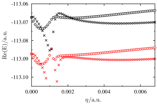
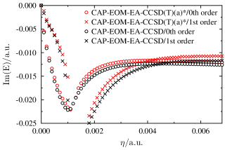
Figure 1: Real (left) and imaginary (right) energy of the ${}^{2}\Pi$ shape resonance of CO^- as a function of CAP strength computed at the CAP-EOM-EA-CCSD and -CCSD(T)(a)* levels of theory using the aug-cc-pVTZ+6s6p6d(C) basis set.

Since triples excitations do not change the positions and widths of shape resonance substantially, one may wonder if it possible to save computer time by determining the optimal CAP strength at the EOM-EA-CCSD level of theory followed by a single CAP-EOM-EA-CCSD(T)(a)* calculation. This is appears to be a valid approach given the very similar optimal CAP strengths obtained with CAP-EOM-EA-CCSD and -CCSD(T)(a)* (see supplementary material) and is further substantiated by the fact that both methods produce similar $\eta$-trajectories. This is documented in Figure 1, which displays $\eta$-trajectories for CO^- as a representative example.

Overall, one can conclude from Table 2 that triples excitations make a minor but in many cases non-negligible impact on positions and widths of shape resonances. In particular, resonance positions change to a similar extent as attachment energies of bound EA states but in the opposite direction. These numerical findings confirm the expectation that resonances with dominant single-attachment character should be described accurately within the EOM-EA-CCSD approximation.

Further trends observed in Table 2, i.e., with respect to basis-set size and the first-order correction are in line with previous findings and need not be discussed in detail. It is, however, worth noting that there are considerable discrepancies between the best theoretical estimates in Table 2 and the corresponding experimental values. For example, the CAP-EOM-EA-CCSD(T)(a)*/aug-cc-pVQZ+6s6p6d(C) results for N${}_{2}^{-}$ including the first-order correction are still 0.1 eV and 0.14 eV away from the fixed-nuclei estimate obtained through a fit to experimental data (E = 2.32 eV, $\Gamma$ = 0.41 eV).berman83 For CO^-, the difference is even larger: The CAP-EOM-EA-CCSD(T)(a)*/aug-cc-pVQZ+6s6p6d(C) values are E = 1.915 eV and $\Gamma$ = 0.657 eV whereas a fit to experimental data yielded E = 1.50 eV and $\Gamma$ = 0.75–0.80 eV.zubek77 ; zubek79 The situation is similar for the other resonances, but the comparison is more difficult for polyatomic species where fixed-nuclei estimates are harder to deduce from experimental data. From Table 2 it is clear that higher-order electron correlation does not provide a sufficient explanation for these discrepancies. Rather, incompleteness of the one-electron basis set may explain part of the difference as resonance positions and widths obtained with the modified aug-cc-pVQZ basis set are likely not yet converged. Also, results obtained at the same level of correlation treatment but using other techniques than CAPs, for example, complex basis functions white17 or the stabilization method falcetta14 are significantly different in some cases.

As a final remark to Table 2, an ambiguity in the determination of the optimal CAP strength for N${}_{2}^{-}$/aug-cc-pVTZ+6s6p6d(C) should be addressed. Two minima in both $\eta\,dE/d\eta$ and $\eta\,dU/d\eta$ are found for this particular system and basis set. The values included in Table 2 conform to results obtained with the other basis sets, but the other set of values, i.e., the ones included as a footnote to Table 2, are closer to the estimate inferred from experimental data and were also reported in Ref. 16. A rigorous solution to this ambiguity would demand the use of another basis set, but for the present purpose, i.e., investigating the impact of triples excitations, this did not seem to be necessary.

As a further application, the potential energy curve of the $\sigma^{*}$ resonance of F${}_{2}^{-}$ and its conversion into a bound anion were studied at the CAP-EOM-EA-CCSD and -CCSD(T)(a)* levels of theory. The bound part of the potential energy curve was additionally computed with EOM-EA-CCSDT. This is documented in Figure 2. While triples excitations do not change the description of F${}_{2}^{-}$ qualitatively, this application illustrates some further aspects of the CAP-EOM-CCSD(T)(a)* method. First, the conversion from temporary to bound anion is not described consistently. At R(FF) = 1.4 Å, the anion is computed to be lower in energy than the neutral molecule, but one still obtains a finite resonance width of about 0.03 eV. If the Schrödinger equation was solved exactly, the resonance width would become zero at the same bond distance where the potential curves of F${}_{2}^{-}$ and F₂ cross. This feature is preserved in CAP-EOM-CCSD where a temporary anion and its parent state are obtained as eigenfunctions of the same Hamiltonian jagau14 , but not in CAP-EOM-CCSD(T)(a)* due to the correction of the target-state energy according to Eq. (10).

Moreover, the bound part of the F${}_{2}^{-}$ potential energy curve in Figure 2 demonstrates that EOM-EA-CCSD(T)(a)* reproduces EOM-EA-CCSDT total energies well, but it is also seen that the deviation grows with increasing bond length. In fact, at R(FF) = 1.6 Å EOM-EA-CCSD(T)(a)* overestimates the attachment energy already by about 0.09 eV relative to EOM-EA-CCSDT, whereas the methods agree up to 0.01 eV at R(FF) = 1.4 Å. This indicates that the increasing multiconfigurational character of neutral F₂ at stretched bond lengths is not fully captured within the CCSD(T)(a) approximation.

V Application to Feshbach Resonances

As an example of a Feshbach resonance, the ${}^{2}\Sigma^{+}$ state of CO^- at around 10 eV was investigated. This resonance arises through attachment of a $3s\,\sigma_{g}$ electron to the $b\;^{3}\Sigma^{+}$ or the $B\;^{1}\Sigma^{+}$ Rydberg state of neutral CO, but lies energetically below both these parent states so that it can decay only through a two-electron process. In a CAP-EOM-CC treatment based on the ground state of neutral CO as reference, the resonance wave function is dominated by a double excitation and it can be anticipated that CAP-EOM-EA-CCSD places the resonance significantly too high in energy, i.e., above its parent states turning it into a core-excited shape resonance. Whether CAP-EOM-EA-CCSD(T)(a)* produces the correct energetic order is less clear and investigated here.

For a number of reasons, the ${}^{2}\Sigma^{+}$ resonance of CO^- represents a good test case for exploratory calculations: Firstly, reliable experimental data about its position (10.04 eV) and width (0.04 eV) have been reported schulz73 and, secondly, its wave function is largely dominated by the aforementioned single configuration. This is in contrast to Feshbach resonances in medium-sized molecules where configuration mixing can entail appreciable single-attachment character. However, describing electron attachment to Rydberg states requires some changes to the computational protocol established for valence shape resonances:zuev14 The d-aug-cc-pVXZ basis sets woon94 have to be used instead of aug-cc-pVXZ to obtain converged energies for the parent Rydberg states and moreover, the CAP onset has to be chosen much larger than the spatial extent of the neutral ground state and also that of the parent states in order to limit the perturbation of the latter states to an acceptable level.

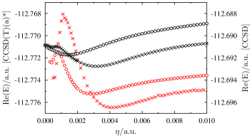
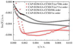
Figure 3: Real (left) and imaginary (right) energy of the ${}^{2}\Sigma^{+}$ Feshbach resonance of CO^- as a function of CAP strength computed at the CAP-EOM-EA-CCSD and -CCSD(T)(a)* levels of theory using the d-aug-cc-pVTZ+6s6p(C) basis set. Note the different energy scales for the two methods in the left panel.

Figure 3 displays $\eta$-trajectories for the ${}^{2}\Sigma^{+}$ resonance of CO^- obtained with CAP-EOM-EA-CCSD and CAP-EOM-EA-CCSD(T)(a)* using the d-aug-cc-pVTZ+6s6p(C) basis set. The differences between the curves illustrate that including triples excitations changes the description of this system qualitatively. At the CAP-EOM-EA-CCSD level, the resonance position and width are obtained as 12.38 eV and 0.17 eV. Since the $b\;^{3}\Sigma^{+}$ parent state is placed at 10.54 eV by EOM-EE-CCSD, the decay via a one-electron process is possible, which explains the unphysically large width. At the CAP-EOM-EA-CCSD(T)(a)* level, the resonance position drops to 10.58 eV and the deviation from the experimental value decreases from over 2 eV to 0.54 eV. However, despite this improvement, the description is still qualitatively wrong because the resonance is above its parent state, which is placed at 10.32 eV by EOM-EE-CCSD(T)(a)*. Consequently, the resonance width is again unphysically large (0.33 eV).

This failure illustrates that CAP-EOM-EA-CCSD(T)(a)* results cannot be trusted when triples excitations induce a qualitative change in the wave function. It is, however, not surprising because the method is explicitly designed for the treatment of states with single excitation/attachment character.matthews16 The perturbative analysis of $\Delta E$ (Eqs. (10)–(12)) assumes that $R_{1}$ contributes at zeroth order but $R_{2}$ only at first order, which is not the case for Feshbach resonances.

A consistent solution to this problem is likely afforded by the full inclusion of triples excitations, i.e., by CAP-EOM-EA-CCSDT. This entails, however, considerably increased computational cost and is beyond the scope of the present work. Alternatively, the parent triplet Rydberg state could be used as reference state in an EOM-CCSD treatment similar to what has been done for resonances of DNA bases in the context of the stabilization method.fennimore16 Such an approach would provide a more balanced treatment as the Feshbach resonance is of single-attachment character and the ground state of the neutral molecule is described through a spin-flipping single excitation, but it is state-specific in the sense that different resonances of the same system are described based on different reference states.

VI Concluding Remarks

In this article, electronic resonances have been studied for the first time beyond the EOM-CCSD approximation. To avoid the high cost of full EOM-CCSDT, triples excitations are taken into account in a non-iterative manner. Since none of the methods proposed for doing so has been applied previously to the EA variant of EOM-CC, benchmark calculations for several bound electron-attached states were carried out first with EOM-EA-CCSDT as reference point.

EOM-EA-CCSD* and EOM-EA-CCSD(fT), which correct only target states, do not yield accurate attachment energies, although significant improvements over EOM-CCSD have been reported for vertical ionization potentials manohar09 and energy differences between EOM-SF states manohar08 . In contrast, the EOM-EA-CCSD(T)(a)* method, in which the CCSD reference state is corrected for the effect of triples excitations before constructing the similarity-transformed Hamiltonian, reliably improves upon EOM-EA-CCSD attachment energies and is comparable in accuracy to EOM-EA-CC3.

Selected applications of EOM-EA-CCSD(T)(a)* augmented by a CAP to temporary anions with shape-resonance character illustrate that higher-order electron correlation uniformly lowers their positions and widths somewhat, in the case of F${}_{2}^{-}$ even by more than 0.1 eV. The present work thus confirms that CAP-EOM-EA-CCSD describes shape resonances rather accurately, but also demonstrates that the effect of higher excitations is not insignificant in many cases but of similar magnitude as the first-order correction for the CAP perturbation.

While CAP-EOM-EA-CCSD(T)(a)* allows to reliably assess higher-order correlation effects in shape resonances at acceptable computational cost (non-iterative $\mathcal{O}(N^{7})$), results for Feshbach resonances are not satisfactory. As these states are doubly excited with respect to the CC reference state, inclusion of triples excitations changes their wave function qualitatively, which is not captured by CAP-EOM-EA-CCSD(T)(a)*: Feshbach resonances are substantially lowered in energy compared to CAP-EOM-EA-CCSD, but still appear above their parent states and thus described incorrectly as core-excited shape resonances. This demonstrates that a more complete treatment of triples excitations is required to achieve a consistent description of Feshbach resonances and their parent states in the context of EOM-CC.

In sum, CAP-free and CAP-augmented EOM-EA-CCSD(T)(a)* could be established as reliable methods for bound and temporary anions of single-attachment character. Exemplary applications illustrate that triples excitations lower resonance positions and widths and confirm the validity of the CAP-EOM-EA-CCSD approach.

Supplementary Material

See supplementary material for computational details such as molecular structures, and CAP parameters as well as results corresponding to Table 1 and Figure 2.

VII Tables

Table 1: Absolute deviations, mean absolute deviations, and maximum deviations in eV of vertical attachment energies of a test set of 22 molecules computed at various levels of EOM-EA-CC theory from the corresponding EOM-EA-CCSDT values.

	EOM-EA-
basis	CCSD	CCSD*	CCSD(fT)	CCSD(T)(a)*	CC3
	mean deviation
aug-cc-pVDZ	0.021	-0.103	-0.078	-0.006	-0.003
aug-cc-pVTZ	0.014	-0.118	-0.088	-0.008	-0.002
aug-cc-pVQZ	0.011	-0.123	-0.092	-0.011	-0.002
	mean absolute deviation
aug-cc-pVDZ	0.036	0.104	0.082	0.013	0.020
aug-cc-pVTZ	0.041	0.118	0.091	0.014	0.019
aug-cc-pVQZ	0.042	0.123	0.095	0.016	0.018
	maximum deviationa
aug-cc-pVDZ	0.114	0.286	0.271	0.022	0.048
aug-cc-pVTZ	0.147	0.320	0.297	0.025	0.063
aug-cc-pVQZ	0.157	0.329	0.304	0.030	0.067

Table 2: Resonance positions and widths in eV of several valence shape resonances computed with CAP-EOM-EA-CCSD and CAP-EOM-EA-CCSD(T)(a)* using different basis sets.

		Resonance positions				Resonance widths
		without correction for CAP		including first-order		without correction for CAP		including first-order
				correction for CAP				correction for CAP
		CAP-EOM-EA-		CAP-EOM-EA-		CAP-EOM-EA-		CAP-EOM-EA-
Molecule	Basis	CCSD	CCSD(T)(a)*	CCSD	CCSD(T)(a)*	CCSD	CCSD(T)(a)*	CCSD	CCSD(T)(a)*
N${}_{2}^{-}$	aug-cc-pVDZ+6s6p6d(C)	2.782	2.718	2.735	2.674	0.397	0.382	0.267	0.243
N${}_{2}^{-}$	aug-cc-pVTZ+6s6p6d(C)a	2.608	2.556	2.567	2.517	0.373	0.359	0.283	0.259
N${}_{2}^{-}$	aug-cc-pVQZ+6s6p6d(C)	2.510	2.467	2.461	2.412	0.359	0.340	0.300	0.273
CO-	aug-cc-pVDZ+6s6p6d(C)	2.292	2.249	2.161	2.155	0.728	0.697	0.695	0.635
CO-	aug-cc-pVTZ+6s6p6d(C)	2.114	2.105	2.021	2.018	0.675	0.631	0.646	0.591
CO-	aug-cc-pVQZ+6s6p6d(C)	2.023	2.021	1.903	1.915	0.710	0.660	0.715	0.657
C2H${}_{2}^{-}$	aug-cc-pVDZ+6s6p6d(C)	2.871	2.860	2.792	2.786	0.878	0.870	0.613	0.599
C2H${}_{2}^{-}$	aug-cc-pVTZ+6s6p6d(C)	2.689	2.683	2.507	2.505	0.968	0.947	0.863	0.847
C2H${}_{2}^{-}$	aug-cc-pVQZ+6s6p6d(C)	2.452	2.455	2.202	2.207	1.135	1.118	1.009	1.009
CH2O-	aug-cc-pVTZ+6s6p6d(C)	1.256	1.206	1.208	1.163	0.328	0.292	0.279	0.239
CO${}_{2}^{-}$	aug-cc-pVTZ+6s6p6d(A)	4.008	3.997	3.983	3.970	0.214	0.216	0.190	0.182
CH2Cl${}_{2}^{-}$	aug-cc-pVTZ+6s6p(A)	1.941	1.902	2.019	1.975	0.732	0.726	0.565	0.572

VIII Figures

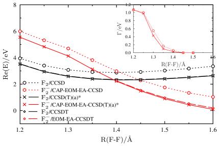
Figure 2: Potential energy curves of F${}_{2}^{-}$ computed at the CAP-EOM-EA-CCSD and -CCSD(T)(a)* levels of theory using the aug-cc-pVTZ+6s6p(A) basis set including first-order correction for the CAP. The corresponding curves of neutral F₂ computed with CCSD and CCSD(T)(a) are also shown.

IX References

References

- (1) T. Helgaker, P. Jørgensen, and J. Olsen, Molecular Electronic Structure Theory (Wiley and Sons, 2000).
- (2) T.-C. Jagau, K.B. Bravaya, and A.I. Krylov, Annu. Rev. Phys. Chem. 68, 525 (2017).
- (3) T. Sommerfeld, U.V. Riss, H.-D. Meyer, L.S. Cederbaum, B. Engels, and H.U. Suter, J. Phys. B 31, 4107 (1998).
- (4) A.F. White, E. Epifanovsky, C.W. McCurdy, and M. Head-Gordon, J. Chem. Phys. 146, 234107 (2017).
- (5) N. Moiseyev, Non-Hermitian Quantum Mechanics (Cambridge University Press, Cambridge, UK, 2011).
- (6) A.U. Hazi and H.S. Taylor, Phys. Rev. A 1, 1109 (1970).
- (7) M. Nestmann and S.D. Peyerimhoff, J. Phys. B 18, 615 (1985).
- (8) J. Horáček, P. Mach, and J. Urban, Phys. Rev. A 82, 032713 (2010).
- (9) J. Aguilar and J.M. Combes, Commun. Math. Phys. 22, 269 (1971).
- (10) E. Balslev and J.M. Combes, Commun. Math. Phys. 22, 280 (1971).
- (11) B. Simon, Phys. Lett. A 71, 211 (1979).
- (12) N. Moiseyev and C. Corcoran, Phys. Rev. A 20, 814 (1979).
- (13) C.W. McCurdy and T. Rescigno, Phys. Rev. Lett. 41, 1364 (1978).
- (14) G. Jolicard and E.J. Austin, Chem. Phys. Lett. 121, 106 (1985).
- (15) U.V. Riss and H.-D. Meyer, J. Phys. B 26, 4503 (1993).
- (16) T.-C. Jagau and A.I. Krylov, J. Chem. Phys. 144, 054113 (2016).
- (17) Z. Benda and T.-C. Jagau, J. Chem. Phys. 146, 031101 (2017).
- (18) A. Ghosh, N. Vaval, and S. Pal, J. Chem. Phys. 136, 234110 (2012).
- (19) K.B. Bravaya, D. Zuev, E. Epifanovsky, and A.I. Krylov, J. Chem. Phys. 138, 124106 (2013).
- (20) D. Zuev, T.-C. Jagau, K.B. Bravaya, E. Epifanovsky, Y. Shao, E. Sundstrom, M. Head-Gordon, and A.I. Krylov, J. Chem. Phys. 141, 024102 (2014). Erratum: 143, 149901 (2015).
- (21) T.-C. Jagau, J. Chem. Phys. 145, 204115 (2016).
- (22) K. Emrich, Nucl. Phys. A 351, 379 (1980).
- (23) J. Geertsen, M. Rittby, and R.J. Bartlett, Chem. Phys. Lett. 164, 57 (1989).
- (24) J.F. Stanton and R.J. Bartlett, J. Chem. Phys. 98, 7029 (1993).
- (25) I. Shavitt and R.J. Bartlett, Many-Body Methods in Chemistry and Physics: MBPT and Coupled-Cluster Theory (Cambridge University Press, Cambridge, 2009).
- (26) A. I. Krylov, Anna. Rev. Phys. Chem. 59, 433 (2008).
- (27) K. Sneskov and O. Christiansen, WIREs: Comput. Mol. Sci. 2, 566 (2012).
- (28) J.F. Stanton and J. Gauss, J. Chem. Phys. 101, 8938 (1994).
- (29) M. Nooijen and R.J. Bartlett, J. Chem. Phys. 102, 3629 (1995).
- (30) T.-C. Jagau and A.I. Krylov, J. Chem. Phys. Lett. 5, 3078 (2014).
- (31) S.A. Kucharski, M. Włoch, M. Musiał, and R.J. Bartlett, 115, 8263 (2001).
- (32) M. Musiałand R.J. Bartlett, J. Chem. Phys. 118, 1128 (2003).
- (33) M. Musiał, S.A. Kucharski, and R.J. Bartlett, J. Chem. Phys. 119, 1901 (2003).
- (34) S. Hirata, M. Nooijen, and R.J. Bartlett, Chem. Phys. Lett. 326, 255 (2000).
- (35) S. Hirata, M. Nooijen, and R.J. Bartlett, Chem. Phys. Lett. 328, 459 (2000).
- (36) S. Hirata, J. Chem. Phys. 121, 51 (2004).
- (37) M. Kállay and J. Gauss, J. Chem. Phys. 121, 9257 (2004).
- (38) O. Christiansen, H. Koch, and P. Jørgensen, J. Chem. Phys. 103, 7429 (1995).
- (39) H. Koch, O. Christiansen, P. Jørgensen, A.M. Sanchez de Merás, and T. Helgaker, J. Chem. Phys. 106, 1808 (1997).
- (40) J.F. Stanton and J. Gauss, J. Chem. Phys. 111, 8785 (1999).
- (41) J.D. Watts and R.J. Bartlett, Chem. Phys. Lett. 233, 81 (1995).
- (42) J.D. Watts and R.J. Bartlett, Chem. Phys. Lett. 258, 581 (1996).
- (43) O. Christiansen, H. Koch, and P. Jørgensen, J. Chem. Phys. 105, 1451 (1996).
- (44) J.F. Stanton and J. Gauss, Theor. Chim. Acta 93, 303 (1996).
- (45) J.C. Saeh and J.F. Stanton, J. Chem Phys. 111, 8275 (1999).
- (46) S. Hirata, M. Nooijen, I. Grabowski, and R.J. Bartlett, J. Chem. Phys. 114, 3919 (2001).
- (47) K. Kowalski and P. Piecuch, J. Chem. Phys. 120, 1715 (2004).
- (48) P.U. Manohar and A.I. Krylov, J. Chem. Phys. 129, 194105 (2008).
- (49) P.U. Manohar, J.F. Stanton, and A.I. Krylov, J. Chem. Phys. 131, 114112 (2009).
- (50) D.A. Matthews and J.F. Stanton, J. Chem. Phys. 145, 124102 (2016).
- (51) K. Raghavachari, G.W. Trucks, J.A. Pople, and M. Head-Gordon, Chem. Phys. Lett. 157, 479 (1989).
- (52) R.J. Bartlett, J.D. Watts, S.A. Kucharski, and J. Noga, Chem. Phys. Lett. 165, 513 (1990).
- (53) S.P.A. Sauer, M. Schreiber, M.R. Silva-Junior, and W. Thiel, J. Chem. Theory Comput. 5, 555 (2009).
- (54) T.J. Watson, V.F. Lotrich, P.G. Szalay, A. Perera, and R.J. Bartlett, J. Phys. Chem. A 117, 2569 (2013).
- (55) D. Kánnár, A. Tajti, and P.G. Szalay, J. Chem. Theory Comput. 13, 202 (2017).
- (56) J. Simons, J. Phys. Chem. A 112, 6401 (2008).
- (57) N. Moiseyev, P.R. Certain, and F. Weinhold, Mol. Phys. 36, 1613 (1978).
- (58) T.-C. Jagau, D. Zuev, K.B. Bravaya, E. Epifanovsky, and A.I. Krylov, J. Phys. Chem. Lett. 5, 310 (2014). Erratum: 6, 3866 (2015).
- (59) Y. Shao, Z. Gan, E. Epifanovsky, A.T.B. Gilbert, M. Wormit, et al., Mol. Phys. 113, 184 (2015).
- (60) E. Epifanovsky, M. Wormit, T. Kuś, A. Landau, D. Zuev, K. Khistyaev, P. Manohar, I. Kaliman, A. Dreuw, and A.I. Krylov, J. Comput. Chem. 34, 2293 (2013).
- (61) L.A. Curtiss, P.C. Redfern, K. Raghavachari, and J.A. Pople, J. Chem. Phys. 109, 42 (1998).
- (62) A.D. Boese and N.C. Handy, J. Chem. Phys. 114, 5497 (2001).
- (63) L.A. Curtiss, P.C. Redfern, and K. Raghavachari, J. Chem. Phys. 123, 124107 (2005).
- (64) R.A. Kendall, T.H. Dunning, and R.J. Harrison, J. Chem. Phys. 96, 6796 (1992).
- (65) D.E. Woon and T.H. Dunning, J. Chem. Phys. 98, 1358 (1993).
- (66) Cfour, a quantum chemical program package written by J.F. Stanton, J. Gauss, L. Cheng, M.E. Harding, D.A. Matthews, P.G. Szalay with contributions from A.A. Auer, R.J. Bartlett, U. Benedikt, C. Berger, D.E. Bernholdt, Y.J. Bomble, O. Christiansen, F. Engel, R. Faber, M. Heckert, O. Heun, C. Huber, T.-C. Jagau, D. Jonsson, J. Jusélius, K. Klein, W.J. Lauderdale, F. Lipparini, T. Metzroth, L.A. M ck, D.P. O’Neill, D.R. Price, E. Prochnow, C. Puzzarini, K. Ruud, F. Schiffmann, W. Schwalbach, C. Simmons, S. Stopkowicz, A. Tajti, J. Vázquez, F. Wang, J.D. Watts and the integral packages MOLECULE (J. Almlöf and P.R. Taylor), Props (P.R. Taylor), Abacus (T. Helgaker, H.J. Aa. Jensen, P. Jørgensen, and J. Olsen), and ECP routines by A. V. Mitin and C. van Wüllen. For the current version, see http://www.cfour.de.
- (67) O. Hino, T. Kinoshita, G. K.-L. Chan, and R.J. Bartlett, J. Chem. Phys. 124, 114311 (2006).
- (68) T. Sommerfeld, B. Bhattarai, V.P. Vysotskiy, and L.S. Cederbaum, J. Chem. Phys. 133, 114301 (2010).
- (69) T.-C. Jagau, D.B. Dao, N.S. Holtgrewe, A.I. Krylov, and R. Mabbs, J. Phys. Chem. Lett. 6, 2786 (2015).
- (70) M. Berman, H. Estrada, L.S. Cederbaum, and W. Domcke, Phys. Rev. A 28, 1363 (1983).
- (71) M. Zubek and C. Szmytkowski, J. Phys. B 10, L27 (1977).
- (72) M. Zubek and C. Szmytkowski, Phys. Lett. 74A, 60 (1979).
- (73) M.F. Falcetta, L.A. Di Falco, D.S. Ackerman, J.C. Barlow, and K.D. Jordan, J. Phys. Chem. A 118, 7489 (2014).
- (74) G.J. Schulz, Rev. Mod. Phys. 45, 423 (1973).
- (75) D.E. Woon and T.H. Dunning, J. Chem. Phys. 100, 2975 (1994).
- (76) M.A. Fennimore and S. Matsika, Phys. Chem. Chem. Phys. 18, 30536 (2016).