Prediction of the CP asymmetry $C_{00}$ in $B^{0}\to D^{0}\overline{D^{0}}$ decay

Abstract

Of all $B\to D\overline{D}$ decays, the $B^{0}\to D^{0}\overline{D^{0}}$ decay has the smallest observed branching ratio as it takes place primarily via the suppressed $W$-exchange diagram. The CP asymmetry for this mode is yet to be measured experimentally. By exploiting the relationship among the decay amplitudes of $B\to D\overline{D}$ decays (using isospin and topological amplitudes) we are able to relate the CP asymmetries and branching ratios by a simple expression. This enables us to predict the CP asymmetry $C_{00}$ in $B^{0}\to D^{0}\overline{D^{0}}$. While the predicted central values of $C_{00}$ are outside the physically allowed region, they are currently associated with large uncertainties owing to the large errors in the measurements of the $B^{0}\to D^{0}\overline{D^{0}}$ branching ratio ($B_{00}$), the other CP asymmetries $C_{+-}$ (of $B^{0}\to D^{+}D^{-}$) and $A_{\text{CP}}$ (of $B^{+}\to D^{+}\overline{D^{0}}$). With a precise determination of $B_{00}$, $C_{+-}$ and $A_{\text{CP}}$, one can use our analytical result to predict $C_{00}$ with a reduced error and compare it with the experimental measurement when it becomes available. The correlation between $B_{00}$ and $C_{00}$ is an interesting aspect that can be probed in ongoing and future particle physics experiments such as LHCb and Belle II.

1 Introduction

It is very well known that violation of CP symmetry, the combined symmetry of charge conjugation (C) and parity (P), is essential for the matter-antimatter asymmetry observed in our Universe Sakharov:1967dj . All observed CP violation in $K$ and $B$ meson decays are successfully explained by the Cabibbo-Kobayashi-Maskawa (CKM) matrix Cabibbo:1963yz ; Kobayashi:1973fv which is a cornerstone of the standard model (SM) of particle physics. However, CP violation as we know in the SM is not sufficient to account for the observed baryon asymmetry in our Universe Gavela:1993ts ; Gavela:1994dt ; Huet:1994jb . Therefore, experimental searches are still going on to find out possibly new sources of CP violation beyond the SM. In this context, study of decays of heavy flavor mesons, especially the $B$ mesons, has played an important role (see Refs. Antonelli:2009ws ; Hocker:2006xb ; Artuso:2015swg ; Gershon:2016fda for some recent reviews). In this work we shall analyze the $B\to D\overline{D}$ decays, in particular $B^{+}\to D^{+}\overline{D^{0}}$, $B^{0}\to D^{0}\overline{D^{0}}$, $B^{0}\to D^{+}D^{-}$ and their CP conjugate processes, with a view to predict the CP-violating parameter $C_{00}$ for $B^{0}\to D^{0}\overline{D^{0}}$, which has not yet been measured experimentally.

In our analysis we shall exploit the isospin symmetry, which is known to be a very useful symmetry in the study of various hadronic decays, most notably in many $B$ meson decays. The existing literature is replete with many interesting studies of double charm decays of the $B$ mesons Bel:2015wha ; Jung:2014jfa ; Mohammadi:2011zz ; Lu:2010gg ; Li:2009xf ; Kim:2008ex ; Gronau:2008ed ; Li:2007rk ; Fleischer:2007zn ; Chen:2005rp ; Datta:2003va ; Xing:1999yx ; Pham:1999fy ; Fleischer:1999nz ; Xing:1998ca ; Sanda:1997pm ; Gronau:1995hm ; Kramer:1994in ; Aleksan:1993qk . Some of these works Jung:2014jfa ; Gronau:2008ed ; Xing:1999yx ; Sanda:1997pm ; Gronau:1995hm also analyze the $B\to D\kern 1.99997pt\overline{\kern-1.99997ptD}{}$ decays in terms of isospin symmetry. The $B\to D\kern 1.99997pt\overline{\kern-1.99997ptD}{}$ decays get contributions from currents that change isospin by $1/2$ and $3/2$. Without making any assumptions regarding the sizes of these contributions, we find out their upper and lower limits. Another useful method to study various hadronic decays of the $B$ and $D$ mesons is the topological diagram approach Zeppenfeld:1980ex ; Chau:1982da ; Chau:1986du ; Chau:1987tk ; Chau:1990ay ; Kim:1998sh ; Chiang:2003jn ; Chiang:2003rb ; Chiang:2003pm ; Chiang:2004nm ; Chiang:2006ih ; Chiang:2007qh ; Chiang:2008vc ; Cheng:2010ry ; Cheng:2010vk ; Cheng:2011qh ; Cheng:2012wr ; Cheng:2012xb ; Cheng:2016ejf . We have used this approach in conjunction with the isospin symmetry to derive a simple expression relating all the branching ratios and CP asymmetries under consideration. This enables us to predict the CP asymmetry $C_{00}$ of the $B^{0}\to D^{0}{\kern-1.60004pt\overline{D^{0}}}$ mode.

This paper is structured as follows. In Sec. 2, we do the isospin decomposition of the concerned decay amplitudes, keeping both $\Delta I=1/2$ and $3/2$ contributions, and provide the upper and lower limits on them. The decay amplitudes are then analyzed from the perspective of topological amplitudes in Sec. 3. This leads to an expression for $C_{00}$ in Sec. 4. It is followed by a relevant numerical analysis in Sec. 5, showing how precision measurements can improve our predictions in the future. Finally we conclude in Sec. 6, highlighting the important results of our analysis.

2 Isospin analysis of $B\to D\overline{D}$ decay amplitudes

2.1 Isospin decomposition of the decay amplitudes

In the $B\to D\kern 1.99997pt\overline{\kern-1.99997ptD}{}$ decays, the initial $B$ meson has isospin $I=\frac{1}{2}$ and the final $D\kern 1.99997pt\overline{\kern-1.99997ptD}{}$ state has isospin $I=0,1$. The effective weak interaction Hamiltonian driving these decays has currents which change the isospin by $1/2$ and $3/2$. Thus the decay amplitudes for the various $B\to D\kern 1.99997pt\overline{\kern-1.99997ptD}{}$ decays can be decomposed under isospin consideration as follows:

$$A_{+-} \equiv\textrm{A}(\kern 1.79993pt\overline{\kern-1.79993ptB}{}^{0}\to D^{+}D^{-})=\frac{1}{\sqrt{2}}\left(A_{1}+B_{1}+A_{0}\right),$$ (1a)

$$A_{00} \equiv\textrm{A}(\kern 1.79993pt\overline{\kern-1.79993ptB}{}^{0}\to D^{0}\overline{D^{0}})=\frac{1}{\sqrt{2}}\left(A_{1}+B_{1}-A_{0}\right),$$ (1b)

$$A_{0-} \equiv\textrm{A}(B^{-}\to D^{0}D^{-})=\frac{1}{\sqrt{2}}\left(2A_{1}-B_{1}\right),$$ (1c)

where $A_{0}$ and $A_{1}$ are the isospin amplitudes facilitated by $\Delta I=1/2$ current to the isospin $I=0,1$ final states respectively and $B_{1}$ denotes the isospin amplitude with $\Delta I=3/2$ current to $I=1$ final state. The conjugate amplitudes are defined as:

$$\overline{A}_{+-} \equiv\textrm{A}(B^{0}\to D^{+}D^{-})=\frac{1}{\sqrt{2}}\left(\overline{A}_{1}+\overline{B}_{1}+\overline{A}_{0}\right),$$ (2a)

$$\overline{A}_{00} \equiv\textrm{A}(B^{0}\to D^{0}\overline{D^{0}})=\frac{1}{\sqrt{2}}\left(\overline{A}_{1}+\overline{B}_{1}-\overline{A}_{0}\right),$$ (2b)

$$\overline{A}_{+0} \equiv\textrm{A}(B^{+}\to D^{+}\overline{D^{0}})=\frac{1}{\sqrt{2}}\left(2\overline{A}_{1}-\overline{B}_{1}\right).$$ (2c)

It is easy to notice from Eqs. (1) and (2) that the amplitudes satisfy the following relations:

$$A_{+-}-A_{00} =\sqrt{2}~{}A_{0},$$ (3a)

$$\overline{A}_{+-}-\overline{A}_{00} =\sqrt{2}~{}\overline{A}_{0},$$ (3b)

$$A_{+-}+A_{00}+2A_{0-} =3\sqrt{2}~{}A_{1},$$ (3c)

$$\overline{A}_{+-}+\overline{A}_{00}+2\overline{A}_{0-} =3\sqrt{2}~{}\overline{A}_{1},$$ (3d)

$$A_{+-}+A_{00}-A_{0-} =\frac{3}{\sqrt{2}}B_{1},$$ (3e)

$$\overline{A}_{+-}+\overline{A}_{00}-\overline{A}_{+0} =\frac{3}{\sqrt{2}}\overline{B}_{1}.$$ (3f)

If one were to neglect $B_{1}$ altogether, one would get the relations $A_{+-}+A_{00}=A_{0-}$ and $\overline{A}_{+-}+\overline{A}_{00}=\overline{A}_{+0}$ as given by Sanda and Xing Sanda:1997pm .

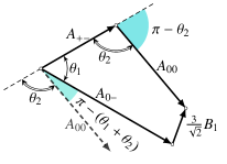
Figure 1: A representative quadrilateral formed by $A_{+-}$, $A_{00}$, $A_{0-}$ and $\frac{3}{\sqrt{2}}B_{1}$, depicting Eq. (3e) graphically (not drawn to scale). Another quadrilateral can be drawn similarly for the conjugate amplitudes, for which we denote the analogous angles by $\theta^{\prime}_{1}$, $\theta^{\prime}_{2}$. The angles $\theta^{\prime}_{1}$ and $\theta^{\prime}_{2}$ can generally be different from $\theta_{1}$ and $\theta_{2}$.

Since amplitudes are complex quantities, they are denoted by vectors in the complex plane. The amplitudes $A_{+-}$, $A_{00}$ and $A_{0-}$ along with $\frac{3}{\sqrt{2}}B_{1}$ (see Eq. (3e)) form a quadrilateral as shown in Fig. 1. Depending on the values for angles $\theta_{1}$ and $\theta_{2}$, the quadrilateral can be either a simple quadrilateral or a self-intersecting quadrilateral. Once again, if $B_{1}=0$, we would get back to the triangles of Sanda and Xing Sanda:1997pm . It is, therefore, interesting to find out how large the magnitudes of $B_{1}$ and $\overline{B}_{1}$ can be per the current experimental observations. Before we get into finding out the limits on $\left|B_{1}\right|$ and $\left|\overline{B}_{1}\right|$, let us first write down the expressions for the experimental observables.

2.2 The experimental observables

The experimental observables we shall use in our analysis are the branching ratios and CP asymmetries which are defined as,

$$B_{+-} =\frac{1}{2}\tau_{0}\frac{\sqrt{\lambda\left(m_{B^{0}}^{2},m_{D^{+}}^{2},m_{D^{+}}^{2}\right)}}{16\pi\,m_{B^{0}}^{3}}\left(\left|A_{+-}\right|^{2}+\left|\overline{A}_{+-}\right|^{2}\right),$$ (4a)

$$B_{00} =\frac{1}{2}\tau_{0}\frac{\sqrt{\lambda\left(m_{B^{0}}^{2},m_{D^{0}}^{2},m_{D^{0}}^{2}\right)}}{16\pi\,m_{B^{0}}^{3}}\left(\left|A_{00}\right|^{2}+\left|\overline{A}_{00}\right|^{2}\right),$$ (4b)

$$B_{\text{ch}} =\frac{1}{2}\tau_{+}\frac{\sqrt{\lambda\left(m_{B^{+}}^{2},m_{D^{+}}^{2},m_{D^{0}}^{2}\right)}}{16\pi\,m_{B^{+}}^{3}}\left(\left|A_{0-}\right|^{2}+\left|\overline{A}_{+0}\right|^{2}\right),$$ (4c)

$$C_{+-} =\frac{\left|A_{+-}\right|^{2}-\left|\overline{A}_{+-}\right|^{2}}{\left|A_{+-}\right|^{2}+\left|\overline{A}_{+-}\right|^{2}},$$ (4d)

$$C_{00} =\frac{\left|A_{00}\right|^{2}-\left|\overline{A}_{00}\right|^{2}}{\left|A_{00}\right|^{2}+\left|\overline{A}_{00}\right|^{2}},$$ (4e)

$$A_{\text{CP}} =\frac{\left|A_{0-}\right|^{2}-\left|\overline{A}_{+0}\right|^{2}}{\left|A_{0-}\right|^{2}+\left|\overline{A}_{+0}\right|^{2}},$$ (4f)

where $m_{i}$ represents the mass of particle $i$, $\tau_{0}$, $\tau_{+}$ are the mean lifetimes of $B^{0}$, $B^{+}$, respectively, and

$$\lambda(x,y,z)=x^{2}+y^{2}+z^{2}-2xy-2yz-2zx~{}.$$

The subscript in $B_{\text{ch}}$ denotes the fact that we are dealing with the decay of a charged $B$ meson in this case.

For simplicity we shall define the ‘scaled’ branching ratios (which have mass dimension 2) and express the CP asymmetries in terms of them as shown below:

$$\mathscr{B}_{+-} =\frac{16\pi m_{B^{0}}^{3}}{\tau_{0}\sqrt{\lambda\left(m_{B^{0}}^{2},m_{D^{+}}^{2},m_{D^{+}}^{2}\right)}}B_{+-}=\frac{1}{2}\left(\left|A_{+-}\right|^{2}+\left|\overline{A}_{+-}\right|^{2}\right),$$ (5a)

$$\mathscr{B}_{00} =\frac{16\pi m_{B^{0}}^{3}}{\tau_{0}\sqrt{\lambda\left(m_{B^{0}}^{2},m_{D^{0}}^{2},m_{D^{0}}^{2}\right)}}B_{00}=\frac{1}{2}\left(\left|A_{00}\right|^{2}+\left|\overline{A}_{00}\right|^{2}\right),$$ (5b)

$$\mathscr{B}_{\text{ch}} =\frac{16\pi m_{B^{+}}^{3}}{\tau_{+}\sqrt{\lambda\left(m_{B^{+}}^{2},m_{D^{+}}^{2},m_{D^{0}}^{2}\right)}}B_{\text{ch}}=\frac{1}{2}\left(\left|A_{0-}\right|^{2}+\left|\overline{A}_{+0}\right|^{2}\right),$$ (5c)

$$C_{+-} =\frac{1}{2\mathscr{B}_{+-}}\left(\left|A_{+-}\right|^{2}-\left|\overline{A}_{+-}\right|^{2}\right),$$ (5d)

$$C_{00} =\frac{1}{2\mathscr{B}_{00}}\left(\left|A_{00}\right|^{2}-\left|\overline{A}_{00}\right|^{2}\right),$$ (5e)

$$A_{\text{CP}} =\frac{1}{2\mathscr{B}_{\text{ch}}}\left(\left|A_{0-}\right|^{2}-\left|\overline{A}_{+0}\right|^{2}\right).$$ (5f)

From the definitions of the observables given in Eq. (5), we can easily obtain the following relations:

$$\left|A_{+-}\right| =\sqrt{\mathscr{B}_{+-}\left(1+C_{+-}\right)}~{},$$ (6a)

$$\left|A_{00}\right| =\sqrt{\mathscr{B}_{00}\left(1+C_{00}\right)}~{},$$ (6b)

$$\left|A_{0-}\right| =\sqrt{\mathscr{B}_{\text{ch}}\left(1+A_{\text{CP}}\right)}~{},$$ (6c)

$$\left|\overline{A}_{+-}\right| =\sqrt{\mathscr{B}_{+-}\left(1-C_{+-}\right)}~{},$$ (6d)

$$\left|\overline{A}_{00}\right| =\sqrt{\mathscr{B}_{00}\left(1-C_{00}\right)}~{},$$ (6e)

$$\left|\overline{A}_{+0}\right| =\sqrt{\mathscr{B}_{\text{ch}}\left(1-A_{\text{CP}}\right)}~{}.$$ (6f)

Since the CP asymmetries must always lie between $-1$ and $1$, i.e., $-1\leqslant C_{00},C_{+-},A_{\text{CP}}\leqslant 1$, the moduli of the amplitudes are always ensured to be positive and real by definition.

2.3 Upper and lower limits on the magnitudes of isospin amplitudes

From Fig. 1 it is easy to show that

$$\left|B_{1}\right|^{2} =\frac{2}{9}\Big{(}\left|A_{+-}\right|^{2}+\left|A_{00}\right|^{2}+\left|A_{0-}\right|^{2}-2\left|A_{+-}\right|\left|A_{00}\right|\cos\theta_{2}$$

$$~{}+2\left|A_{00}\right|\left|A_{0-}\right|\cos\left(\theta_{1}+\theta_{2}\right)-2\left|A_{0-}\right|\left|A_{+-}\right|\cos\theta_{1}\Big{)}.$$ (7)

Considering the conjugate amplitudes, we would get

$$\left|\overline{B}_{1}\right|^{2} =\frac{2}{9}\Big{(}\left|\overline{A}_{+-}\right|^{2}+\left|\overline{A}_{00}\right|^{2}+\left|\overline{A}_{+0}\right|^{2}-2\left|\overline{A}_{+-}\right|\left|\overline{A}_{00}\right|\cos\theta^{\prime}_{2}$$

$$~{}+2\left|\overline{A}_{00}\right|\left|\overline{A}_{+0}\right|\cos\left(\theta^{\prime}_{1}+\theta^{\prime}_{2}\right)-2\left|\overline{A}_{+0}\right|\left|\overline{A}_{+-}\right|\cos\theta^{\prime}_{1}\Big{)},$$ (8)

where the angles $\theta^{\prime}_{1}$, $\theta^{\prime}_{2}$ denote the fact that they are necessarily different from the analogous angles $\theta_{1}$, $\theta_{2}$. Now the limits on $\left|B_{1}\right|$ (and $\left|\overline{B}_{1}\right|$) can be obtained by taking some specific values for the angles $\theta_{1}$ and $\theta_{2}$ of Fig. 1 (or $\theta^{\prime}_{1}$ and $\theta^{\prime}_{2}$), as well as for the moduli of the decay amplitudes, as shown below.

Maximum

The maximum value for $\left|B_{1}\right|$ is obtained when $A_{+-}$, $A_{00}$ and $-A_{0-}$ are all directed along the same direction, i.e., when the angles in Fig. 1 are set to the values $\theta_{1}=\pi=\theta_{2}$,

$$\left|B_{1}\right|^{2}_{\textrm{max}}=\frac{2}{9}\Big{(}\left|A_{+-}\right|+\left|A_{00}\right|+\left|A_{0-}\right|\Big{)}^{2}.$$ (9)

We can consider all the conjugate amplitudes in a similar manner, and this would lead to the maximum for $\left|\overline{B}_{1}\right|$,

$$\left|\overline{B}_{1}\right|^{2}_{\textrm{max}}=\frac{2}{9}\Big{(}\left|\overline{A}_{+-}\right|+\left|\overline{A}_{00}\right|+\left|\overline{A}_{+0}\right|\Big{)}^{2}.$$ (10)

Minimum

There are two interesting scenarios for finding the minimum of $\left|B_{1}\right|^{2}$. In the first case, the quadrilateral is squashed into a straight line (analogous to the situation for maximum), while in the later case, for $\left|B_{1}\right|_{\text{min}}=0$, the quadrilateral is transformed into a triangle. These two cases can be easily distinguished from each other by first arranging the three amplitude moduli in either increasing or decreasing order. Then we take the sum of the two smaller moduli. If the largest modulus is greater than the sum of the two smaller moduli, then the amplitudes can never form a triangle, i.e. $\left|B_{1}\right|_{\textrm{min}}\neq 0$. In the case where the largest modulus is smaller than the sum of the two smaller moduli, the amplitudes can form a triangle resulting in $\left|B_{1}\right|_{\textrm{min}}=0$. When $\left|B_{1}\right|_{\textrm{min}}\neq 0$ we have the following three possibilities,

$$\left|B_{1}\right|^{2}_{\textrm{min}}=\begin{cases}\frac{2}{9}\Big{(}-\left|A_{+-}\right|+\left|A_{00}\right|+\left|A_{0-}\right|\Big{)}^{2}&\textrm{for }\theta_{1}=0=\theta_{2},\\ \frac{2}{9}\Big{(}\left|A_{+-}\right|+\left|A_{00}\right|-\left|A_{0-}\right|\Big{)}^{2}&\textrm{for }\theta_{1}=0,\theta_{2}=\pi,\\ \frac{2}{9}\Big{(}\left|A_{+-}\right|-\left|A_{00}\right|+\left|A_{0-}\right|\Big{)}^{2}&\textrm{for }\theta_{1}=\pi,\theta_{2}=0.\end{cases}$$ (11)

Once again, considering the conjugate amplitudes would give the set of three minima for $\left|\overline{B}_{1}\right|$,

$$\left|\overline{B}_{1}\right|^{2}_{\textrm{min}}=\begin{cases}\frac{2}{9}\Big{(}-\left|\overline{A}_{+-}\right|+\left|\overline{A}_{00}\right|+\left|\overline{A}_{+0}\right|\Big{)}^{2}&\textrm{for }\theta^{\prime}_{1}=0=\theta^{\prime}_{2},\\ \frac{2}{9}\Big{(}\left|\overline{A}_{+-}\right|+\left|\overline{A}_{00}\right|-\left|\overline{A}_{+0}\right|\Big{)}^{2}&\textrm{for }\theta^{\prime}_{1}=0,\theta^{\prime}_{2}=\pi,\\ \frac{2}{9}\Big{(}\left|\overline{A}_{+-}\right|-\left|\overline{A}_{00}\right|+\left|\overline{A}_{+0}\right|\Big{)}^{2}&\textrm{for }\theta^{\prime}_{1}=\pi,\theta^{\prime}_{2}=0.\end{cases}$$ (12)

It is important to note that following steps similar to the ones presented here, it is also possible to give expressions for maximum and minimum of $\left|A_{1}\right|$ and $\left|\overline{A}_{1}\right|$ as follows,

$$\left|A_{1}\right|^{2}_{\textrm{max}} =\frac{1}{18}\Big{(}\left|A_{+-}\right|+\left|A_{00}\right|+2\left|A_{0-}\right|\Big{)}^{2},$$ (13a)

$$\left|\overline{A}_{1}\right|^{2}_{\textrm{max}} =\frac{1}{18}\Big{(}\left|\overline{A}_{+-}\right|+\left|\overline{A}_{00}\right|+2\left|\overline{A}_{+0}\right|\Big{)}^{2},$$ (13b)

$$\left|A_{1}\right|^{2}_{\textrm{min}} =\begin{cases}\frac{1}{18}\Big{(}-\left|A_{+-}\right|+\left|A_{00}\right|+2\left|A_{0-}\right|\Big{)}^{2},\\ \frac{1}{18}\Big{(}\left|A_{+-}\right|+\left|A_{00}\right|-2\left|A_{0-}\right|\Big{)}^{2},\\ \frac{1}{18}\Big{(}\left|A_{+-}\right|-\left|A_{00}\right|+2\left|A_{0-}\right|\Big{)}^{2},\end{cases}$$ (13c)

$$\left|\overline{A}_{1}\right|^{2}_{\textrm{min}} =\begin{cases}\frac{1}{18}\Big{(}-\left|\overline{A}_{+-}\right|+\left|\overline{A}_{00}\right|+2\left|\overline{A}_{+0}\right|\Big{)}^{2},\\ \frac{1}{18}\Big{(}\left|\overline{A}_{+-}\right|+\left|\overline{A}_{00}\right|-2\left|\overline{A}_{+0}\right|\Big{)}^{2},\\ \frac{1}{18}\Big{(}\left|\overline{A}_{+-}\right|-\left|\overline{A}_{00}\right|+2\left|\overline{A}_{+0}\right|\Big{)}^{2}.\end{cases}$$ (13d)

Furthermore, it is trivial to find out the maximum and minimum of $\left|A_{0}\right|$ and $\left|\overline{A}_{0}\right|$,

$$\left|A_{0}\right|^{2}_{\text{max}} =\frac{1}{2}\Big{(}\left|A_{+-}\right|+\left|A_{00}\right|\Big{)}^{2},$$ (14a)

$$\left|A_{0}\right|^{2}_{\text{min}} =\frac{1}{2}\Big{(}\left|A_{+-}\right|-\left|A_{00}\right|\Big{)}^{2},$$ (14b)

$$\left|\overline{A}_{0}\right|^{2}_{\text{max}} =\frac{1}{2}\Big{(}\left|\overline{A}_{+-}\right|+\left|\overline{A}_{00}\right|\Big{)}^{2},$$ (14c)

$$\left|\overline{A}_{0}\right|^{2}_{\text{min}} =\frac{1}{2}\Big{(}\left|\overline{A}_{+-}\right|-\left|\overline{A}_{00}\right|\Big{)}^{2}.$$ (14d)

We shall provide a numerical comparison of the allowed maximum and minimum values for $\left|A_{0}\right|$, $\left|A_{1}\right|$, $\left|B_{1}\right|$, $\left|\overline{A}_{0}\right|$, $\left|\overline{A}_{1}\right|$, $\left|\overline{B}_{1}\right|$ in Sec. 5.

Thus far, we have considered the two possible quadrilaterals separately. However, the amplitudes and their CP conjugate amplitudes are related to one another via the strong and weak phases. In order to do an analysis keeping both strong and weak phases into account, we shall consider the various quark diagrams (also known as topological diagrams) contributing to the $B\to D\kern 1.99997pt\overline{\kern-1.99997ptD}{}$ decays under our consideration.

3 Analysis of $B\to D\overline{D}$ decay amplitudes under diagrammatic approach

3.1 Contributing topological diagrams

The $B\to D\kern 1.99997pt\overline{\kern-1.99997ptD}{}$ decays are facilitated by various topological diagrams, which are enunciated below.

1. The $B^{+}\to D^{+}\overline{D^{0}}$ decay gets contributions from color-allowed tree, $W$-annihilation, QCD-penguin, QCD-penguin exchange, color-suppressed electroweak-penguin and electroweak-penguin exchange diagrams.

2. The $B^{0}\to D^{+}D^{-}$ decay gets contributions from color-allowed tree, $W$-exchange, QCD-penguin, QCD-penguin exchange, QCD-penguin annihilation, color-suppressed electroweak-penguin, electroweak-penguin exchange and electroweak-penguin annihilation diagrams.

3. The $B^{0}\to D^{0}\overline{D^{0}}$ decay gets contributions from $W$-exchange, QCD-penguin annihilation and electroweak-penguin annihilation diagrams.

Therefore, theoretically the branching ratio for $B^{0}\to D^{0}\overline{D^{0}}$ is expected to be smaller than those for $B^{+}\to D^{+}\overline{D^{0}}$ and $B^{0}\to D^{+}D^{-}$ Li:2007rk . Contribution of each topological diagram is denoted by an amplitude, the topological amplitude, multiplied by appropriate CKM matrix elements. All $B\to D\kern 1.99997pt\overline{\kern-1.99997ptD}{}$ decay amplitudes under our consideration are proportional to $V_{Ub}^{*}V_{Ud}$ where $U$ can be $u,c,t$ and $V$ denotes the CKM matrix. The relevant CKM unitarity condition for $B\to D\kern 1.99997pt\overline{\kern-1.99997ptD}{}$ decays is

$$V^{*}_{ub}V_{ud}+V^{*}_{cb}V_{cd}+V^{*}_{tb}V_{td}=0.$$ (15)

In our subsequent discussions, we shall use the weak phase $\beta$ which is an angle of the unitarity triangle associated with Eq. (15) and defined as

$$\beta=\text{arg}\left(-\frac{V^{*}_{cb}V_{cd}}{V^{*}_{tb}V_{td}}\right).$$ (16)

3.2 Decomposition of decay amplitudes in terms of topological diagrams

If we break up our decay amplitudes by using the topological amplitudes with relevant CKM matrix elements, then we can relate the isospin amplitudes with combinations of topological amplitudes. In general, we can use the unitarity condition and the definition of weak phase $\beta$ to write down the decay amplitudes as follows,

$$A_{+-} =A^{\prime}_{+-}+A^{\prime\prime}_{+-}~{}e^{i\beta},$$ (17a)

$$A_{00} =A^{\prime}_{00}+A^{\prime\prime}_{00}~{}e^{i\beta},$$ (17b)

$$A_{0-} =A^{\prime}_{0-}+A^{\prime\prime}_{0-}~{}e^{i\beta},$$ (17c)

where

$$A^{\prime}_{+-} =\frac{1}{\sqrt{2}}\left(\left|A^{\prime}_{1}\right|e^{i\delta_{1}}+\left|A^{\prime}_{0}\right|e^{i\delta_{0}}+\left|B^{\prime}_{1}\right|\right),$$ (18a)

$$A^{\prime\prime}_{+-} =\frac{1}{\sqrt{2}}\left(\left|A^{\prime\prime}_{1}\right|e^{i\delta_{1}}+\left|A^{\prime\prime}_{0}\right|e^{i\delta_{0}}+\left|B^{\prime\prime}_{1}\right|\right),$$ (18b)

$$A^{\prime}_{00} =\frac{1}{\sqrt{2}}\left(\left|A^{\prime}_{1}\right|e^{i\delta_{1}}-\left|A^{\prime}_{0}\right|e^{i\delta_{0}}+\left|B^{\prime}_{1}\right|\right),$$ (18c)

$$A^{\prime\prime}_{00} =\frac{1}{\sqrt{2}}\left(\left|A^{\prime\prime}_{1}\right|e^{i\delta_{1}}-\left|A^{\prime\prime}_{0}\right|e^{i\delta_{0}}+\left|B^{\prime\prime}_{1}\right|\right),$$ (18d)

$$A^{\prime}_{0-} =\frac{1}{\sqrt{2}}\left(2\left|A^{\prime}_{1}\right|e^{i\delta_{1}}-\left|B^{\prime}_{1}\right|\right),$$ (18e)

$$A^{\prime\prime}_{0-} =\frac{1}{\sqrt{2}}\left(2\left|A^{\prime\prime}_{1}\right|e^{i\delta_{1}}-\left|B^{\prime\prime}_{1}\right|\right),$$ (18f)

with $A^{\prime}_{0}$, $A^{\prime\prime}_{0}$, $A^{\prime}_{1}$, $A^{\prime\prime}_{1}$, $B^{\prime}_{1}$, $B^{\prime\prime}_{1}$ being various components of the isospin amplitudes, each with a distinct decomposition in terms of the contributing topological amplitudes, and $\delta_{1}$, $\delta_{0}$ being the strong phases measured with respect to $B_{1}$. The decomposition of various components of the isospin amplitudes of Eq. (18) in terms of the topological amplitudes are as follows:

$$A^{\prime}_{0} =\frac{1}{\sqrt{2}}\left(-T_{c}+E_{c}\right),$$ (19a)

$$A^{\prime\prime}_{0} =\frac{1}{3\sqrt{2}}\Big{(}3E_{t}+3P+2P^{C}_{EW}+3P\!E-P\!E_{EW}-12P\!A-5P\!A_{EW}\Big{)},$$ (19b)

$$A^{\prime}_{1} =\frac{1}{3\sqrt{2}}\left(-3T_{c}+E_{c}+2A_{c}\right),$$ (19c)

$$A^{\prime\prime}_{1} =\frac{1}{3\sqrt{2}}\Big{(}-E_{t}-2A_{t}+3P+2P^{C}_{EW}+3P\!E+P\!E_{EW}+P\!A_{EW}\Big{)},$$ (19d)

$$B^{\prime}_{1} =\frac{\sqrt{2}}{3}\left(E_{c}-A_{c}\right),$$ (19e)

$$B^{\prime\prime}_{1} =\frac{\sqrt{2}}{3}\left(-E_{t}+A_{t}+P\!A_{EW}-P\!E_{EW}\right),$$ (19f)

where the tree $T$, $W$-annihilation $A$, $W$-exchange $E$ are the topologies with no quark loop, and QCD-penguin $P$, QCD-penguin annihilation $P\!A$, QCD-penguin exchange $P\!E$, color-suppressed electroweak-penguin $P^{C}_{EW}$, electroweak-penguin annihilation $P\!A_{EW}$ and electroweak-penguin exchange $P\!E_{EW}$ are the dominant one loop topologies with top quark in the loop. Note that for the no-loop topologies $N\in\{T,E,A\}$ the subscript in Eq. (19) has the meaning that $N_{x}=NV_{xb}^{*}V_{xd}$, and in the one loop topologies $L\in\{P,P\!A,P\!E,P^{C}_{EW},P\!A_{EW},P\!E_{EW}\}$ in Eq. (19) the factor $V_{tb}^{*}V_{td}$ is implicitly present. The up and charm quark contributions to one loop topologies can also be considered in a similar manner. However, they do not affect our analysis. Finally, the decay amplitudes for the conjugate processes are obtained by switching the sign of the weak phase $\beta$ in Eq. (17),

$$\overline{A}_{+-} =A^{\prime}_{+-}+A^{\prime\prime}_{+-}e^{-i\beta},$$ (20a)

$$\overline{A}_{00} =A^{\prime}_{00}+A^{\prime\prime}_{00}e^{-i\beta},$$ (20b)

$$\overline{A}_{0-} =A^{\prime}_{0-}+A^{\prime\prime}_{0-}e^{-i\beta}.$$ (20c)

We shall now look at the consequences of the two amplitude decompositions we have carried out.

4 Consequence of decomposition of amplitudes using isospin and topological diagrams

Starting from Eqs. (17), (18) and (20) one can write down the observables $\mathscr{B}_{+-}$, $C_{+-}$, $\mathscr{B}_{00}$, $C_{00}$, $\mathscr{B}_{\text{ch}}$ and $A_{\text{CP}}$ in terms of the various isospin amplitudes, strong and weak phases. The expressions for the CP asymmetries are given by

$$C_{+-} =\frac{\sin\beta}{\mathscr{B}_{+-}}\Bigg{(}-\left(\left|A^{\prime\prime}_{0}\right|\left|B^{\prime}_{1}\right|-\left|A^{\prime}_{0}\right|\left|B^{\prime\prime}_{1}\right|\right)\sin\delta_{0}-\left(\left|A^{\prime\prime}_{1}\right|\left|B^{\prime}_{1}\right|-\left|A^{\prime}_{1}\right|\left|B^{\prime\prime}_{1}\right|\right)\sin\delta_{1}$$

$$\hskip 170.71652pt-\left(\left|A^{\prime\prime}_{0}\right|\left|A^{\prime}_{1}\right|-\left|A^{\prime}_{0}\right|\left|A^{\prime\prime}_{1}\right|\right)\sin\left(\delta_{0}-\delta_{1}\right)\Bigg{)},$$ (21a)

$$C_{00} =\frac{\sin\beta}{\mathscr{B}_{00}}\Bigg{(}\left(\left|A^{\prime\prime}_{0}\right|\left|B^{\prime}_{1}\right|-\left|A^{\prime}_{0}\right|\left|B^{\prime\prime}_{1}\right|\right)\sin\delta_{0}-\left(\left|A^{\prime\prime}_{1}\right|\left|B^{\prime}_{1}\right|-\left|A^{\prime}_{1}\right|\left|B^{\prime\prime}_{1}\right|\right)\sin\delta_{1}$$

$$\hskip 170.71652pt+\left(\left|A^{\prime\prime}_{0}\right|\left|A^{\prime}_{1}\right|-\left|A^{\prime}_{0}\right|\left|A^{\prime\prime}_{1}\right|\right)\sin\left(\delta_{0}-\delta_{1}\right)\Bigg{)},$$ (21b)

$$A_{\text{CP}} =\frac{2\sin\beta}{\mathscr{B}_{\text{ch}}}\left(\left|A^{\prime\prime}_{1}\right|\left|B^{\prime}_{1}\right|-\left|A^{\prime}_{1}\right|\left|B^{\prime\prime}_{1}\right|\right)~{}\sin\delta_{1}.$$ (21c)

With these results, it is straightforward to obtain the following important expression which relates all the known branching ratios and CP asymmetries for the $B\to D\kern 1.99997pt\overline{\kern-1.99997ptD}{}$ decays:

$$\mathscr{B}_{+-}~{}C_{+-}+\mathscr{B}_{00}~{}C_{00}+\mathscr{B}_{\text{ch}}~{}A_{\text{CP}}=0.$$ (22)

This simple relation can be used to predict $C_{00}$ which is currently not measured experimentally,

$$C_{00} =-\frac{1}{\mathscr{B}_{00}}\bigg{(}\mathscr{B}_{+-}~{}C_{+-}+\mathscr{B}_{\text{ch}}~{}A_{\text{CP}}\bigg{)}$$

$$=-\frac{\sqrt{\lambda\left(m_{B^{0}}^{2},m_{D^{0}}^{2},m_{D^{0}}^{2}\right)}}{B_{00}}\left(\frac{B_{+-}C_{+-}}{\displaystyle\sqrt{\lambda\left(m_{B^{0}}^{2},m_{D^{+}}^{2},m_{D^{+}}^{2}\right)}}+\frac{B_{\text{ch}}A_{\text{CP}}}{\displaystyle\sqrt{\lambda\left(m_{B^{+}}^{2},m_{D^{+}}^{2},m_{D^{0}}^{2}\right)}}\left(\frac{m_{B^{+}}^{3}}{m_{B^{0}}^{3}}\frac{\tau_{0}}{\tau_{+}}\right)\right).$$ (23)

We note that this result arises when both isospin amplitudes and topological amplitudes are considered together. After getting the expression for $C_{00}$ it is pertinent that we do the required numerical analysis taking the current experimental data into account.

5 Numerical analysis

5.1 Experimental data

For $B\to D\kern 1.99997pt\overline{\kern-1.99997ptD}{}$ decays, we have results from many experiments Aaij:2016yip ; Aaij:2013fha ; Rohrken:2012ta ; Fratina:2007zk ; Aubert:2008ah ; Adachi:2008cj ; Aubert:2006ia . But for consistency, we consider the PDG PDG data in this paper and for comparison we take into account the recent results on $C_{+-}$ by LHCb Aaij:2016yip and by the heavy flavor averaging group, HFLAV Amhis:2016xyh as well. The experimental data are,

$$B_{+-} =(2.11\pm 0.18)\times 10^{-4},$$ (24a)

$$C_{+-} =\begin{cases}-0.22\pm 0.24&\text{(PDG)},\\ 0.26^{+0.18}_{-0.17}(\textrm{stat})\pm 0.02(\textrm{syst})&\text{(LHCb)},\\ -0.13\pm 0.10&\text{(HFLAV)},\end{cases}$$ (24b)

$$B_{00} =(1.4\pm 0.7)\times 10^{-5},$$ (24c)

$$B_{\text{ch}} =(3.8\pm 0.4)\times 10^{-4},$$ (24d)

$$A_{\text{CP}} =-0.03\pm 0.07.$$ (24e)

It is important to note that the errors in $B_{00}$, $C_{+-}$ and $A_{\text{CP}}$ are large enough to make them consistent with $0$ within $2\sigma$, and the CP asymmetry $C_{00}$ is not yet measured experimentally. It must be noted that in the averaging done by PDG for $C_{+-}$ both 2007 Fratina:2007zk and 2012 Rohrken:2012ta Belle results are considered, while the HFLAV averaging for $C_{+-}$ considers only 2012 Rohrken:2012ta Belle result. Since, the 2012 Belle result supersedes the 2007 Belle result (see Ref. Rohrken:2012ta ), we consider the HFLAV averaging of $C_{+-}$ to be more reliable than the one done by PDG.

5.2 Estimates of magnitudes of decay amplitudes

Using the experimental data from Eq. (24) in the expressions for the moduli of the various amplitudes as given in Eq. (6) we get the following estimates, with the errors combined in quadrature,

$$\left|A_{+-}\right| =\begin{cases}\left(1.637\pm 0.261\right)\times 10^{-4}\textrm{ eV}&\text{(PDG)},\\ \left(2.080\pm 0.174\right)\times 10^{-4}\textrm{ eV}&\text{(LHCb)},\\ \left(1.729\pm 0.124\right)\times 10^{-4}\textrm{ eV}&\text{(HFLAV)},\end{cases}$$ (25a)

$$\left|\overline{A}_{+-}\right| =\begin{cases}\left(2.047\pm 0.261\right)\times 10^{-4}\textrm{ eV}&\text{(PDG)},\\ \left(1.594\pm 0.174\right)\times 10^{-4}\textrm{ eV}&\text{(LHCb)},\\ \left(1.970\pm 0.124\right)\times 10^{-4}\textrm{ eV}&\text{(HFLAV)},\end{cases}$$ (25b)

$$\left|A_{0-}\right| =\left(2.358\pm 0.150\right)\times 10^{-4}\textrm{ eV},$$ (25c)

$$\left|\overline{A}_{+0}\right| =\left(2.430\pm 0.152\right)\times 10^{-4}\textrm{ eV}.$$ (25d)

Since $C_{00}$ is not yet known experimentally, we can only predict $\left|A_{00}\right|$ and $\left|\overline{A}_{00}\right|$ in the physically allowed range of $C_{00}$. This is shown in Fig. 2. We find that

$$0\leqslant\left|A_{00}\right|,\left|\overline{A}_{00}\right|\leqslant\left(0.674\pm 0.168\right)\times 10^{-4}\textrm{ eV}.$$ (26)

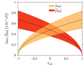
Figure 2: Predictions of $\left|A_{00}\right|$ and $\left|\overline{A}_{00}\right|$ over the physically allowed range of $C_{00}$. The colored band denotes the $1\sigma$ error.

5.3 Numerical limits on magnitudes of isospin amplitudes

The shaded regions in Figs. 3, 4 and 5 show the allowed maxima and minima of the magnitudes of isospin amplitudes: $\left|A_{0}\right|$, $\left|\overline{A}_{0}\right|$, $\left|A_{1}\right|$, $\left|\overline{A}_{1}\right|$, $\left|B_{1}\right|$ and $\left|\overline{B}_{1}\right|$, in the physically allowed range of $C_{00}$, and as permitted by the current experimental data taken from PDG PDG , LHCb Aaij:2016yip and HFLAV Amhis:2016xyh respectively. We have used Eqs. (9) and (10) to find out the maximum values of $\left|B_{1}\right|$ and $\left|\overline{B}_{1}\right|$ respectively. For the minimum values we have three cases for both Eq. (11) and Eq. (12) and we have shown in the plots the absolute minimum out of the three minima possibilities for both $\left|B_{1}\right|$ and $\left|\overline{B}_{1}\right|$. The maxima and minima of $\left|A_{1}\right|$ and $\left|\overline{A}_{1}\right|$ were evaluated in a similar manner using Eq. (13). Finally, for the maxima and minima of $\left|A_{0}\right|$ and $\left|\overline{A}_{0}\right|$, we have made use of Eq. (14).

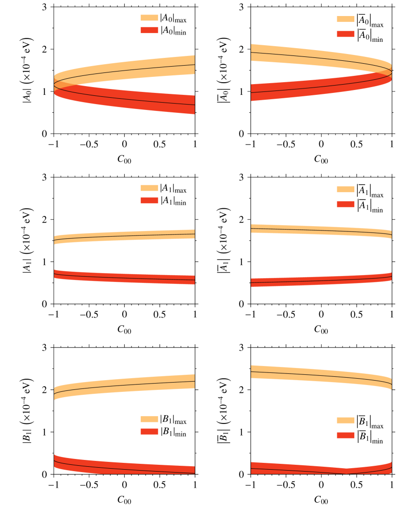
Figure 3: Comparison of upper and lower limits on $\left|A_{0}\right|$, $\left|\overline{A}_{0}\right|$, $\left|A_{1}\right|$, $\left|\overline{A}_{1}\right|$, $\left|B_{1}\right|$ and $\left|\overline{B}_{1}\right|$ assuming that $C_{00}$ lies between $-1$ and $1$. Here we have used the PDG data PDG for $C_{+-}$. It is easy to notice that the allowed ranges for $\left|B_{1}\right|$ and $\left|\overline{B}_{1}\right|$ are comparable with that of $\left|A_{1}\right|$ and $\left|\overline{A}_{1}\right|$ respectively.

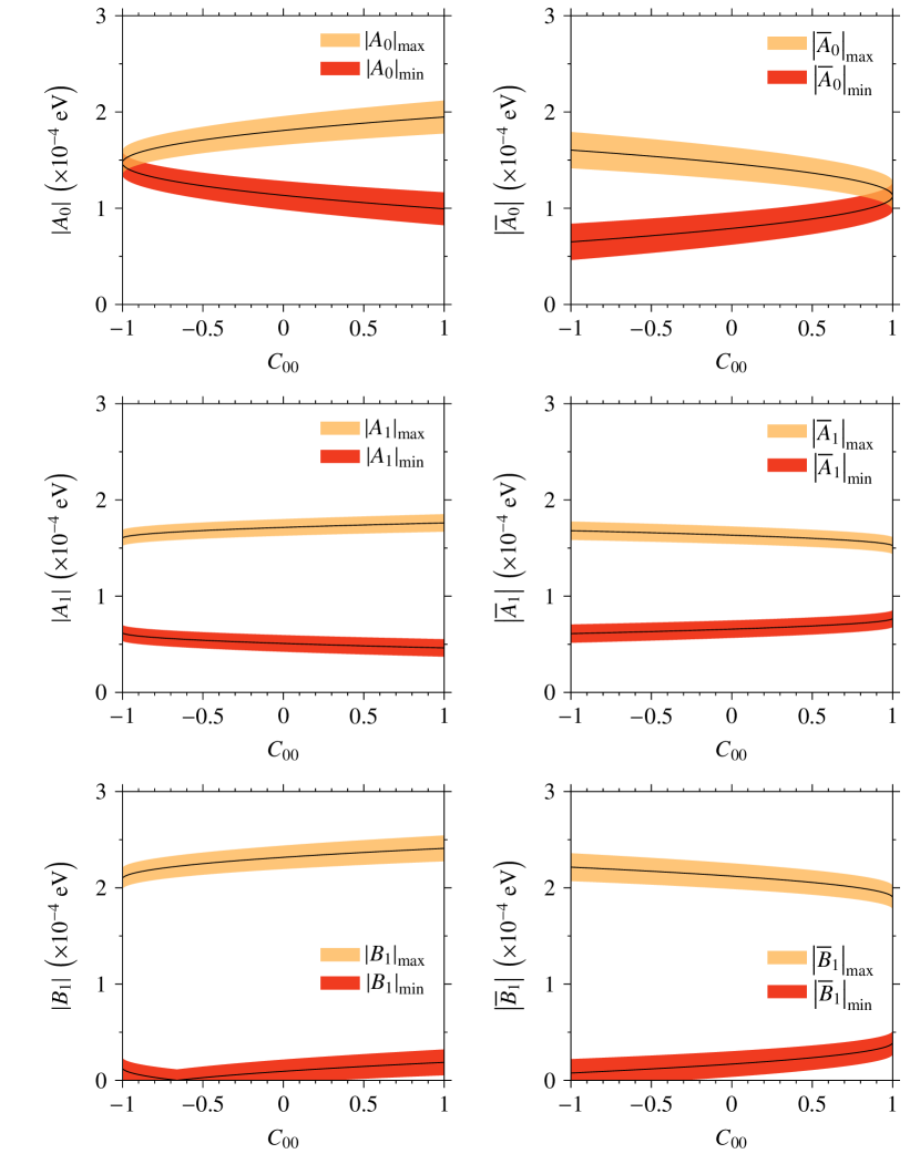
Figure 4: Same as Fig. 3 except for using $C_{+-}$ as reported by the LHCb collaboration Aaij:2016yip .

Figure 5: Same as Fig. 3 except for using $C_{+-}$ as reported by the HFLAV Amhis:2016xyh .

5.4 Predictions for $C_{00}$

In the absence of an experimental measurement, we can use Eq. (23) to predict a value for $C_{00}$, which with current experimental data is

$$C_{00}=\begin{cases}4.081\pm 4.530&\textrm{(using PDG data)},\\ -3.172\pm 3.638&\textrm{(using LHCb data)},\\ 2.721\pm 2.699&\textrm{(using HFLAV result)}.\end{cases}$$ (27)

Clearly, the central value of the predicted $C_{00}$ lies outside the physically allowed region for $C_{00}$: $-1\leqslant C_{00}\leqslant 1$. However, the large error in $C_{00}$ essentially owes its origin to the fact that $B_{00}$, $C_{+-}$ and $A_{\text{CP}}$ are consistent with zero within $2\sigma$. Therefore, precise measurements of $B_{00}$, $C_{+-}$, $A_{\text{CP}}$ and an experimental determination of the CP asymmetry $C_{00}$ would be very interesting.

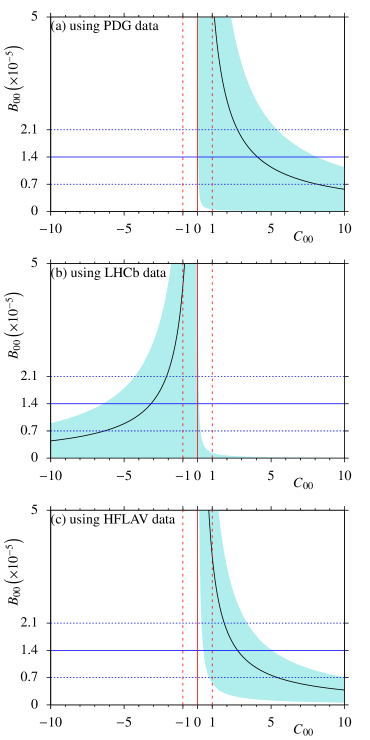
Figure 6: Comparison of predicted value of $B_{00}$ from Eq. (28) with the measured value of $B_{00}=(1.4\pm 0.7)\times 10^{-5}$, with $C_{+-}$ taken from the PDG average, LHCb measurement and the HFLAV average. The shaded region shows the $1\sigma$ error on the predicted mean value of $B_{00}$ given by the black curve. The experimental value of $B_{00}$ lies within the blue dashed lines at $1\sigma$. Here for the purpose of illustration, we have included the unphysical regions of $C_{00}$. The physically allowed region for $C_{00}$ is within the red dashed lines.

From Eq. (23), one can write down the following expression for $B_{00}$:

$$B_{00}=-\frac{\sqrt{\lambda\left(m_{B^{0}}^{2},m_{D^{0}}^{2},m_{D^{0}}^{2}\right)}}{C_{00}}\left(\frac{B_{+-}C_{+-}}{\displaystyle\sqrt{\lambda\left(m_{B^{0}}^{2},m_{D^{+}}^{2},m_{D^{+}}^{2}\right)}}+\frac{B_{\text{ch}}A_{\text{CP}}}{\displaystyle\sqrt{\lambda\left(m_{B^{+}}^{2},m_{D^{+}}^{2},m_{D^{0}}^{2}\right)}}\left(\frac{m_{B^{+}}^{3}}{m_{B^{0}}^{3}}\frac{\tau_{0}}{\tau_{+}}\right)\right).$$ (28)

Using Eq. (28) we can predict the value of $B_{00}$ in the physically allowed region of $C_{00}$. In Fig. 6 we provide a comparison of the predicted behaviour of $B_{00}$ with the experimental measurement.

5.5 Discussion on numerical analysis

If we consider the mean values alone in Eq. (25) and the upper limit from Eq. (26), then we can arrange the moduli of decay amplitudes in the following order,

$$\left|A_{0-}\right|>\left|A_{+-}\right|>\left|A_{00}\right|,~{}\text{and}~{}\left|\overline{A}_{+0}\right|>\left|\overline{A}_{+-}\right|>\left|\overline{A}_{00}\right|,$$

consistent with the observation that $B_{\text{ch}}>B_{+-}>B_{00}$. Moreover, considering the mean values again we find that,

$$\left|A_{+-}\right|+\left|A_{00}\right|<\left|A_{0-}\right| \text{(for PDG data)},$$

$$\left|A_{+-}\right|+\left|A_{00}\right|>\left|A_{0-}\right| \text{(for LHCb and HFLAV data)},$$

$$\left|\overline{A}_{+-}\right|+\left|\overline{A}_{00}\right|<\left|\overline{A}_{+0}\right| \text{(for LHCb data)},$$

$$\left|\overline{A}_{+-}\right|+\left|\overline{A}_{00}\right|>\left|\overline{A}_{+0}\right|$$ (for PDG and HFLAV data)

which lead to the possibilities $\left|B_{1}\right|\neq 0$, $\left|B_{1}\right|=0$, $\left|\overline{B}_{1}\right|\neq 0$ and $\left|\overline{B}_{1}\right|=0$ respectively. However, if we consider the $1\sigma$ errors, both $\left|B_{1}\right|$ and $\left|\overline{B}_{1}\right|$ can vanish for all cases under our consideration. This can be easily seen from Figs. 3, 4 and 5. From these figures we also observe that the allowed ranges for $\left|A_{1}\right|$, $\left|\overline{A}_{1}\right|$, $\left|B_{1}\right|$ and $\left|\overline{B}_{1}\right|$ are all very similar. It must be noted that we have $9$ free parameters in our formalism ($A^{\prime}_{0}$, $A^{\prime\prime}_{0}$, $A^{\prime}_{1}$, $A^{\prime\prime}_{1}$, $B^{\prime}_{1}$, $B^{\prime\prime}_{1}$, $\delta_{0}$, $\delta_{1}$, $\beta$) and currently we have experimental information about $\sin\beta$ and $5$ out of the $6$ observables (viz., $B_{+-}$, $B_{00}$, $B_{\text{ch}}$, $C_{+-}$, $A_{\text{CP}}$ and not yet $C_{00}$). Therefore, it is not possible, at current, to do a meaningful $\chi^{2}$-analysis and look for best fit values of the isospin amplitudes in order to make a comparison. Even adding the observable $S_{+-}$ (and $S_{00}$ which is not yet measured) does not make any difference, since the addition of these observables also leads to consideration of additional free parameters. Nevertheless, as experimental data becomes available in the future for all possible observables related to the decay modes under our consideration, it would eventually be possible to do a meaningful $\chi^{2}$-analysis and study the individual isospin amplitudes and strong phases in a clear manner.

As we have noted earlier the predicted value of $C_{00}$ (see Eq. (27)) has the mean value completely outside the physically allowed region with large error which makes it consistent with zero within about $1\sigma$. However, if we analyze Fig. 6 we find that by looking in the window of observed range for $B_{00}$, within $1\sigma$ standard deviation, the region $C_{00}\geqslant 0$ is favoured by both PDG and HFLAV data, while both positive and negative values of $C_{00}$ are allowed if we consider LHCb data alone. If we go to higher standard deviations, the full physical range of $C_{00}$ is allowed by the existing data, consistent with Eq. (27). It must be noted that, from Eq. (28) as well as from Fig. 6 it is clear that the prediction for $B_{00}$ has a singularity at $C_{00}=0$. Thus, if $C_{00}$ is experimentally measured to be non-zero, then we expect $B_{00}$ to have larger value than the currently measured value which is consistent with zero at $2\sigma$ level. This is by assuming that the other measurements, as given in Eq. (24), remain unchanged. A larger $B_{00}$ would imply significant contribution from diagrams such as the $W$-exchange diagrams. Thus, this interplay of $B_{00}$ and $C_{00}$ measurements could lead to some potential search for new physics.

We would like to emphasize that the large errors in Eq. (27) can be reduced if we have precise measurements of $B_{00}$, $C_{+-}$ and $A_{\text{CP}}$ which are all currently consistent with zero within $2\sigma$. To illustrate this point, let us consider a scenario in which future experimental analyses with larger data sets give us values of $B_{00}$, $C_{+-}$ and $A_{\text{CP}}$ with their central values unchanged but with reduced errors. This scenario is hypothetical because future experiments will not only shrink the errors but also shift the central values in general. Nevertheless, to put our emphasis on precise measurement of $B_{00}$, $C_{+-}$ and $A_{\text{CP}}$ on a quantitative basis, we can probe the prospect of Belle II experiment which is expected to have 50 times larger integrated luminosity than Belle Belle:2017wmf . In such a scenario, we can naïvely expect the errors on $B_{00}$, $C_{+-}$ and $A_{\text{CP}}$ (taking the HFLAV averages as an example) to get scaled down by a factor of roughly $1/\sqrt{50}$. Using our method, such reduced errors on the above-mentioned observables will render an error of about $0.4$ for $C_{00}$. If the central value of $C_{00}$ is still significantly larger than 1 compared to this new error, it will be an interesting hint of new physics at work. It is also important to note that as $B^{0}\to D^{0}{\kern-1.60004pt\overline{D^{0}}}$ involves the $W$-exchange, QCD-penguin annihilation and electroweak-penguin annihilation diagrams, a more precise determination of observables related to this mode provides an ideal means to probe the strong dynamics in these topological amplitudes.

6 Conclusions

In this paper we have analyzed the $B\to D\kern 1.99997pt\overline{\kern-1.99997ptD}{}$ decay modes in terms of isospin amplitudes and the topological amplitudes. This leads us to predict the value of the CP asymmetry $C_{00}$ in $B^{0}\to D^{0}\overline{D^{0}}$ mode to be $4.081\pm 4.530$, or $-3.172\pm 3.638$, or $2.721\pm 2.699$ depending on whether we use the $C_{+-}$ value as reported by PDG, or LHCb, or HFLAV, respectively. Though the central values are all outside the physically allowed range for $C_{00}$, the predictions are consistent with zero due to large errors. The errors in $C_{00}$ predictions are large because of very large errors in $B_{00}$, $C_{+-}$ and $A_{\text{CP}}$ all of which enter the expression for $C_{00}$. With more precise measurements of $B_{00}$, $C_{+-}$ and $A_{\text{CP}}$, and an experimental observation of $C_{00}$ it would be possible to make a better comparison of the observation with prediction using Eq. (23). Further experimental results from the time-dependent decay rates for the modes $B^{0}\to D^{0}\overline{D^{0}}$ and $B^{0}\to D^{+}D^{-}$ would pave the way for a complete meaningful $\chi^{2}$-analysis which can be used to determine the contributions of various isospin amplitudes, as well as strong phases that take part in the $B\to D\kern 1.99997pt\overline{\kern-1.99997ptD}{}$ decays under consideration. Furthermore, the correlation between $B_{00}$ and $C_{00}$ is an interesting aspect that can be probed in ongoing and future particle physics experiments such as LHCb and Belle II.

- (1) A. D. Sakharov, “Violation of CP invariance, C asymmetry, and baryon asymmetry of the universe,” Pisma Zh. Eksp. Teor. Fiz. 5, 32 (1967) [JETP Lett. 5, 24 (1967)] [Sov. Phys. Usp. 34, 392 (1991)] [Usp. Fiz. Nauk 161, 61 (1991)].
- (2) N. Cabibbo, “Unitary Symmetry and Leptonic Decays,” Phys. Rev. Lett. 10, 531 (1963).
- (3) M. Kobayashi and T. Maskawa, “CP Violation in the Renormalizable Theory of Weak Interaction,” Prog. Theor. Phys. 49, 652 (1973).
- (4) M. B. Gavela, P. Hernandez, J. Orloff and O. Pene, “Standard model CP violation and baryon asymmetry,” Mod. Phys. Lett. A 9, 795 (1994).
- (5) M. B. Gavela, P. Hernandez, J. Orloff, O. Pene and C. Quimbay, “Standard model CP violation and baryon asymmetry. Part 2: Finite temperature,” Nucl. Phys. B 430, 382 (1994) doi:10.1016/0550-3213(94)00410-2 [hep-ph/9406289].
- (6) P. Huet and E. Sather, “Electroweak baryogenesis and standard model CP violation,” Phys. Rev. D 51, 379 (1995).
- (7) M. Antonelli et al., “Flavor Physics in the Quark Sector,” Phys. Rept. 494, 197 (2010).
- (8) A. Hocker and Z. Ligeti, “CP violation and the CKM matrix,” Ann. Rev. Nucl. Part. Sci. 56, 501 (2006).
- (9) M. Artuso, G. Borissov and A. Lenz, “CP violation in the system,” Rev. Mod. Phys. 88, no. 4, 045002 (2016).
- (10) T. Gershon and V. V. Gligorov, “ violation in the system,” Rept. Prog. Phys. 80, no. 4, 046201 (2017).
- (11) L. Bel, K. De Bruyn, R. Fleischer, M. Mulder and N. Tuning, “Anatomy of decays,” JHEP 1507, 108 (2015).
- (12) M. Jung and S. Schacht, “Standard model predictions and new physics sensitivity in decays,” Phys. Rev. D 91, no. 3, 034027 (2015).
- (13) B. Mohammadi and H. Mehraban, “Final state interaction in ,” JHEP 1107, 089 (2011).
- (14) L. X. Lu, Z. J. Xiao, S. W. Wang and W. J. Li, “The Double charm decays of B Mesons in the mSUGRA model,” Commun. Theor. Phys. 56, 125 (2011).
- (15) R. H. Li, X. X. Wang, A. I. Sanda and C. D. Lu, “Decays of meson to two charmed mesons,” Phys. Rev. D 81, 034006 (2010).
- (16) C. S. Kim, R. M. Wang and Y. D. Yang, “Studying Double Charm Decays of and Mesons in the MSSM with -parity Violation,” Phys. Rev. D 79, 055004 (2009).
- (17) M. Gronau, J. L. Rosner and D. Pirjol, “Small amplitude effects in and related decays,” Phys. Rev. D 78, 033011 (2008).
- (18) Y. Li and J. Hua, “Study of pure annihilation decays ,” Chin. Phys. C 32, 781 (2008).
- (19) R. Fleischer, “Exploring violation and penguin effects through and ,” Eur. Phys. J. C 51, 849 (2007).
- (20) C. H. Chen, C. Q. Geng and Z. T. Wei, “Factorization and polarization in two charmed-meson decays,” Eur. Phys. J. C 46, 367 (2006).
- (21) A. Datta and D. London, “Extracting from and decays,” Phys. Lett. B 584, 81 (2004).
- (22) Z. z. Xing, “ violation in and decays,” Phys. Rev. D 61, 014010 (1999).
- (23) X. Y. Pham and Z. z. Xing, “ asymmetries in and : wave dilution, penguin and rescattering effects,” Phys. Lett. B 458, 375 (1999).
- (24) R. Fleischer, “Extracting from and ,” Eur. Phys. J. C 10, 299 (1999).
- (25) Z. z. Xing, “Measuring violation and testing factorization in and decays,” Phys. Lett. B 443, 365 (1998).
- (26) A. I. Sanda and Z. z. Xing, “Towards determining with ,” Phys. Rev. D 56, 341 (1997).
- (27) M. Gronau, O. F. Hernandez, D. London and J. L. Rosner, “Decays of mesons to two pseudoscalars in broken symmetry,” Phys. Rev. D 52, 6356 (1995).
- (28) G. Kramer, W. F. Palmer and H. Simma, “ violation and strong phases from penguins in and decays,” Z. Phys. C 66, 429 (1995).
- (29) R. Aleksan, A. Le Yaouanc, L. Oliver, O. Pene and J. C. Raynal, “The Decay in the heavy quark limit and tests of violation,” Phys. Lett. B 317, 173 (1993).
- (30) D. Zeppenfeld, “ Relations for Meson Decays,” Z. Phys. C 8, 77 (1981).
- (31) L. L. Chau, “Quark Mixing in Weak Interactions,” Phys. Rept. 95, 1 (1983).
- (32) L. L. Chau and H. Y. Cheng, “Quark Diagram Analysis of Two-body Charm Decays,” Phys. Rev. Lett. 56, 1655 (1986).
- (33) L. L. Chau and H. Y. Cheng, “Analysis of Exclusive Two-Body Decays of Charm Mesons Using the Quark Diagram Scheme,” Phys. Rev. D 36, 137 (1987).
- (34) L. L. Chau, H. Y. Cheng, W. K. Sze, H. Yao and B. Tseng, “Charmless nonleptonic rare decays of mesons,” Phys. Rev. D 43, 2176 (1991) Erratum: [Phys. Rev. D 58, 019902 (1998)].
- (35) C. S. Kim, D. London and T. Yoshikawa, “Using decays to determine the angles and ,” Phys. Rev. D 57, 4010 (1998).
- (36) C. W. Chiang and J. L. Rosner, “New physics contributions to the decay,” Phys. Rev. D 68, 014007 (2003).
- (37) C. W. Chiang, M. Gronau and J. L. Rosner, “Two body charmless B decays involving eta and eta-prime,” Phys. Rev. D 68, 074012 (2003).
- (38) C. W. Chiang, M. Gronau, Z. Luo, J. L. Rosner and D. A. Suprun, “Charmless decays using flavor SU(3) symmetry,” Phys. Rev. D 69, 034001 (2004).
- (39) C. W. Chiang, M. Gronau, J. L. Rosner and D. A. Suprun, “Charmless decays using flavor SU(3) symmetry,” Phys. Rev. D 70, 034020 (2004).
- (40) C. W. Chiang and Y. F. Zhou, “Flavor SU(3) analysis of charmless meson decays to two pseudoscalar mesons,” JHEP 0612, 027 (2006).
- (41) C. W. Chiang and Y. F. Zhou, “Flavor SU(3) analysis of charmless decays,” J. Phys. Conf. Ser. 110, 052056 (2008).
- (42) C. W. Chiang, M. Gronau and J. L. Rosner, “Examination of Flavor SU(3) in , Decays,” Phys. Lett. B 664, 169 (2008).
- (43) H. Y. Cheng and C. W. Chiang, “Two-body hadronic charmed meson decays,” Phys. Rev. D 81, 074021 (2010)
- (44) H. Y. Cheng and C. W. Chiang, “Hadronic D decays involving even-parity light mesons,” Phys. Rev. D 81, 074031 (2010).
- (45) H. Y. Cheng and S. Oh, “Flavor symmetry and QCD factorization in and decays,” JHEP 1109, 024 (2011).
- (46) H. Y. Cheng and C. W. Chiang, “Direct CP violation in two-body hadronic charmed meson decays,” Phys. Rev. D 85, 034036 (2012) Erratum: [Phys. Rev. D 85, 079903 (2012)].
- (47) H. Y. Cheng and C. W. Chiang, “SU(3) symmetry breaking and CP violation in decays,” Phys. Rev. D 86, 014014 (2012).
- (48) H. Y. Cheng, C. W. Chiang and A. L. Kuo, “Global analysis of two-body decays within the framework of flavor symmetry,” Phys. Rev. D 93, no. 11, 114010 (2016).
- (49) R. Aaij et al. [LHCb Collaboration], “Measurement of violation in decays,” Phys. Rev. Lett. 117, no. 26, 261801 (2016).
- (50) R. Aaij et al. [LHCb Collaboration], “First observations of , and decays,” Phys. Rev. D 87, no. 9, 092007 (2013).
- (51) M. Rohrken et al. [Belle Collaboration], “Measurements of Branching Fractions and Time-dependent CP Violating Asymmetries in Decays,” Phys. Rev. D 85, 091106 (2012).
- (52) S. Fratina et al. [Belle Collaboration], “Evidence for CP violation in decays,” Phys. Rev. Lett. 98, 221802 (2007).
- (53) B. Aubert et al. [BaBar Collaboration], “Measurements of time-dependent CP asymmetries in - decays,” Phys. Rev. D 79, 032002 (2009).
- (54) I. Adachi et al. [Belle Collaboration], “Measurement of the branching fraction and charge asymmetry of the decay and search for ,” Phys. Rev. D 77, 091101 (2008).
- (55) B. Aubert et al. [BaBar Collaboration], “Measurement of branching fractions and -violating charge asymmetries for -meson decays to , and implications for the Cabibbo-Kobayashi-Maskawa angle ,” Phys. Rev. D 73, 112004 (2006).
- (56) C. Patrignani et al. (Particle Data Group), Chin. Phys. C, 40, 100001 (2016) and 2017 update.
- (57) Y. Amhis et al., “Averages of -hadron, -hadron, and -lepton properties as of summer 2016,” arXiv:1612.07233 [hep-ex].
- (58) L. Li Gioi [Belle and Belle II Collaborations], “Belle achievements and Belle II prospects for CP violation,” J. Phys. Conf. Ser. 873, no. 1, 012022 (2017).