Coexistence of antiferromagnetism and topological superconductivity on the honeycomb lattice Hubbard model

Abstract

Motivated by the recent numerical simulations for doped $t$-$J$ model on the honeycomb lattice, we study superconductivity of singlet and triplet pairing on the honeycomb lattice Hubbard model. We show that a superconducting state with coexisting spin-singlet and spin-triplet pairings is induced by the antiferromagnetic order near half filling. The superconducting state we obtain has a topological phase transition that separates a topologically trivial state and a nontrivial state with Chern number two. Possible experimental realization of such a topological superconductivity is also discussed.

I Introduction

Antiferromagnetism and superconductivity are two key phenomena that appear in high temperature superconductors such as cuprates and iron pnictides [1, 2, 3, 4, 5, 6, 7, 8, 9, 10, 11, 12]. In these systems, interaction creates strong magnetic correlations between electrons and leads to a Mott insulator with antiferromagnetic (AFM) order for undoped cuprates and a bad metal with spin density wave (SDW) order for undoped iron pnictides. Upon doping, the magnetic order disappears and superconductivity (SC) takes place. There have been many discussions on the roles played by these two different orders in the phase diagram. On one hand, it has been argued that magnetic fluctuations play an essential role for the mechanism of high temperature superconductivity, especially in a class of theory based on the novel concept of spin-charge separation and RVB scenario [1, 2, 13, 4], where the metastable spin liquid state(which has a short-range AFM order and is energetically close to the AFM state) naturally leads to SC order upon doping. On the other hand, the concept of quantum criticality suggests that the AFM order or the SDW order is a competing order that suppresses SC order [3, 14, 15, 16, 17, 18, 19]. Although the strongly coupling pictures seem to be very elegant and attractive, so far there is no controlled way to perform microscopic calculations starting from realistic models, e.g., Hubbard model with strong repulsive interactions. Therefore, to understand the interplay between AFM order and SC order is still an open question and it plays a crucial role for understanding the underlying physics in these systems.

In this paper, we propose an effective Ginzburg-Landau theory to study the interplay between AFM order and SC order in the honeycomb lattice Hubbard model, which has been intensively studied recently. At half filling, antiferromagnetism in the undoped honeycomb lattice has been studied using quantum Monte Carlo and other analytical methods [20, 21, 22]. In these studies an AFM phase is found above a critical on-site repulsion $U_{c}$. Upon doping, SC order has been found in the doped model using various methods [23, 24, 25, 26, 27], where different pairing symmetries have been found, including spin-singlet $s$-wave, $d+id$-wave pairing and spin-triplet $p$-wave, $f$-wave pairing.

In a recent Grassmann tensor product state(GTPS) numerical study of the honeycomb lattice $t$-$J$ model [28], a phase with coexisting AFM and SC orders has been found at low doping levels. Particularly, the superconducting state that coexists with AFM order has both $d+id$ spin-singlet and $p+ip$ spin-triplet pairings. However, the GTPS numerical study could not tell us whether the $d+id$/$p+ip$ SC state is topologically trivial or nontrivial, since the numerical results can not distinguish strong pairing and weak pairing cases. We find that the proposed Ginzburg-Landau theory can naturally explain such a result based on the trilinear term which naturally couples AFM, $d+id$ spin-singlet pairing and $p+ip$ spin-triplet pairing. Moreover, the proposed trilinear term also suggests a topological phase transition that separates a topologically trivial state and a nontrivial state with Chern number two. Although the microscopical origin of such a trilinear term is still unclear, we believe that it serves as a starting point for honeycomb lattice $t$-$J$ and has the potential to reveal the key mechanism for the emergence of SC order in honeycomb lattice $t$-$J$ and Hubbard models.

In Sec. II, we study the AFM order in the honeycomb lattice Hubbard model using mean field theory. At half filling, the band structure has two Dirac cones, and the on-site Coulomb repulsion favors a commensurate AFM order. Due to the vanishing density of states of the Dirac cones, a finite interaction strength is required to open an AFM gap on the Dirac cones. At finite doping, the Dirac points grow into small pocket-like Fermi surfaces. We first calculated the magnetic susceptibility and show that the magnetic order is still commensurate. We then calculated the phase diagram of the AFM phase in mean field approximation. A highlight of the phase diagram is that at finite doping the AFM order is suppressed at low temperature due to the fact that the commensurate order does not gap the Fermi surface, and at large enough doping the system reenters a paramagnetic state at low temperature while there is an AFM phase at intermediate temperatures. In Sec. III we study the coexistence of AFM order and SC order using Ginzburg-Landau theory. We first show that because of the symmetry of the honeycomb lattice, a spin-singlet pairing and a spin-triplet pairing actually has the same lattice symmetry transformation. Consequently the three order parameters of AFM and spin-singlet and triplet SC can together form a trilinear coupling term in the low energy effective Hamiltonian. Therefore when there is a coexistence of AFM and SC orders, the pairing naturally has both spin-singlet and spin-triplet pairings. Moreover, in the presence of an AFM order, the trilinear term becomes a quadratic coupling between two SC order parameters and therefore the AFM order enhances SC order. In Sec. IV we discuss the topological classification of the three-order coexisting state. We first identify a possible topological phase transition point where the quasiparticle gap vanishes on one Dirac node. Then by calculating the change of Berry phase connection near the nodal point across the phase transition, we conclude that the Chern number of the SC state indeed changes across the transition point and it separates two topologically different SC states, which are topologically trivial and nontrivial respectively.

II Antiferromagnetic order

In this section we study the AFM order in the honeycomb lattice Hubbard model using mean field approximation. We start with the following model,

$$H=-t\sum_{\langle ij\rangle\alpha}\left(c_{i\alpha}^{\dagger}c_{j\alpha}+\text{h. c.}\right)+U\sum_{i}n_{i\uparrow}n_{i\downarrow}.$$ (1)

The first term in the above Hamiltonian can be diagonalized in Fourier space as the following,

$$H_{t}=-t\sum_{k\alpha}\bar{c}_{k\alpha}^{\dagger}\begin{pmatrix}0&\xi_{k}^{\ast}\\ \xi_{k}&0\end{pmatrix}\bar{c}_{k\alpha},$$ (2)

where $\bar{c}_{k\alpha}=\begin{pmatrix}c_{Ak\alpha}&c_{Bk\alpha}\end{pmatrix}^{T}$ represents electron operators on two sites A and B in a unit cell (see Fig. 1), and $\alpha=\uparrow,\downarrow$ denotes the electron spin. The function $\xi_{k}=1+e^{ik_{1}}+e^{ik_{2}}$, and $k_{i}=\bm{k}\cdot\bm{a}_{i}$ is the $i$-th component of the momentum with respect to the two primitive translation vector $\bm{G}_{1,2}$ of the triangular lattice, as shown in Fig. 1. (Here, the superscript $T$ denotes matrix transpose.) It is well-known that this represents a band structure with two Dirac cones located at $\pm\bm{K}=\pm\left(\frac{2\pi}{3},-\frac{2\pi}{3}\right)$ (the momentum is given in the reciprocal basis of $\bm{G}_{1,2}$). The second term provides an on-site Coulomb repulsion and when $U$ is much greater than $t$ one can restrict oneself in the single-occupied subspace and obtain a $t$-$J$ model with antiferromagnetic interaction on nearest neighbor bonds as a low-energy effective model. Hence at large enough $U$ the system has an antiferromagnetic ground state.

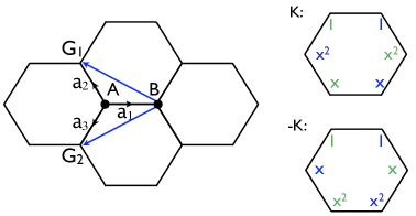
Figure 1: Structure of honeycomb lattice. In the left panel the three vectors $\bm{a}_{i}$ shows the direction of nearest neighbor bonds, and $\bm{G}_{1,2}$ are two primitive vectors of the triangular Bravais lattice. In the right panel the pairing symmetries at two Dirac points are shown, where $x=e^{i2\pi/3}$, and blue and green letters represent positive and negative phases respectively.

Here we study this AFM order in mean field approximation. We introduce the following SDW order parameter,

$$\bm{M}_{i}=\left<\bm{S}_{i}\right>$$ (3)

Plugging this into equation (1), the $U$ term can be decomposed into the following form in mean field approximation,

$$Un_{i\uparrow}\cdot n_{i\downarrow}=\frac{U}{2}n_{i}-2\bm{M}_{i}\cdot\bm{S}_{i}+\frac{\bm{M}_{i}^{2}}{U}$$ (4)

Note, that the first term merely shifts the chemical potential of the system by $\frac{U}{2}$ and shall be ignored.

As discussed in Appendix A, we consider a commensurate order

$$\bm{M}_{i}=(-)^{i}M_{0}\bm{e}_{z}$$ (5)

where $(-)^{i}$ equals to 1 on sublattice A and $-1$ on sublattice B. With the mean field decomposition in equation (4), the Hamiltonian can be written in momentum space as

$$H_{\text{MFT}}=\sum_{k\alpha}\bar{c}_{k\alpha}^{\dagger}\begin{pmatrix}-\mu+\alpha M_{0}&-t\xi_{k}^{\ast}\\ -t\xi_{k}&-\mu-\alpha M_{0}\end{pmatrix}\bar{c}_{k\alpha}+\frac{N}{U}M_{0}^{2},$$ (6)

Using the Hamiltonian described in equation (6), we plot the mean field phase diagram through numerically minimizing the Hamiltonian with respect to the AFM order parameter $M_{z}$ at a fixed doping $x$. Results of $M_{z}$ as a function of temperature at different doping levels are plotted in Fig. 2, and the phase diagram determined from this self-consistent calculation is plotted in Fig. 3.

Figure 2: AFM order parameter as a function of temperature at different doping levels. The plot was calculated with $U=3t$. Both $T$ and $M_{z}$ axes are in units of $t$.

Figure 3: Mean field phase diagram of the Hubbard model. The solid line is where the AFM order parameter $M_{z}$ vanishes, and it separates the AFM phase and the paramagnetic (PM) phase. The dashed line is where $M_{z}=\mu$, and it separates the two superconducting phases with different topological classifications in the weak coupling limit. This is discussed in Sec. IV.

At zero doping, the $M_{z}$ curve has a typical parabolic shape, showing a paramagnetic high temperature phase and an antiferromagnetic low temperature phase separated by a continuous phase transition. At finite doping, the AFM order is generally suppressed as the commensurate order cannot gap the Fermi surface. The suppression is stronger at low temperature and weaker at high temperature, since at high temperature the Fermi surface is not quite clear when $T\geq T_{F}$. At doping levels $x=0.02$ and $x=0.025$, the magnetic order is completely suppressed at low temperatures and the system reenters the paramagnetic phase at a lower critical temperature. For these two dopings, the antiferromagnetic phase only exists between two critical temperatures. At the doping level $x=0.0256$, the antiferromagnetic phase disappears as the two critical temperatures merge. Of course, according to the Mermin-Wagner theorem, the AFM order will be killed by quantum fluctuation at finite temperature for strictly 2D systems. However, for realistic material, the interlayer coupling will always stabilize AFM order at finite temperature. Therefore, the above phase diagram is still reasonable for realistic systems and can be improved by considering both quantum fluctuations and interlayer couplings.

III Coexistence of three orders

In the previous section, we see that the Hubbard model on the honeycomb lattice develops commensurate AFM order at zero and small dopings. In this section, we argue that this AFM order will induce superconducting order with mixed singlet and triplet pairings.

One interesting feature observed in the numerical study of Ref. 28 is that the superconducting state has both spin-singlet and spin-triplet pairings. In a lattice with inversion symmetry, singlet and triplet pairing order parameters have even and odd parity under inversion symmetry operation respectively and therefore do not mix. However, the honeycomb lattice does not have inversion symmetry and therefore in general allows the mixing of singlet and triplet pairing order parameters. Both the singlet and triplet pairing order parameters found in the aforementioned numerical study have a 120-degree spatial pattern: The phase on the bonds of the honeycomb lattice rotates by 120 degrees around the center of each hexagon, as shown in Fig. 4. The singlet pairing symmetry is the same as the $d+id$ pairing obtained in other researches [29, 25].

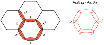
(a) Spin-singlet pairing.

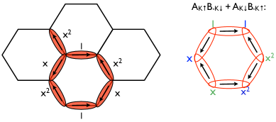
(b) Spin-triplet pairing.

Figure 4: Spin-singlet and spin-triplet pairing symmetry. The complex pairing amplitudes are noted along the bonds, where $x=e^{i2\pi/3}$.

The same spatial pattern of the two pairing symmetries implies the mixing of spin-singlet and spin-triplet pairing in the presence of AFM order. Since the spin-singlet and spin-triplet pairings have the same spatial pattern, they transform in the same way under three-fold rotation. Therefore it is easy to check that the following combination of the three order parameters is invariant under all symmetry transformations including spin rotation, time reversal lattice symmetry transformations, and electromagnetic U(1) gauge symmetry transformation,

$$H_{3}=\lambda_{3}\bm{M}\cdot\Delta_{s}^{\ast}\bm{\Delta}_{t}+\text{h. c.},$$ (7)

and therefore is allowed to appear in the low-energy effective Hamiltonian of the system. In Eq. (7) $\Delta_{s}$ and $\bm{\Delta}_{t}$ denote the superconducting order parameter of spin-singlet and spin-triplet pairing respectively, where the latter is a spin-1 vector. The presence of this trilinear term implies that once two of the three order parameters become nonzero, the third one will be automatically induced, as the symmetry that the third order breaks has already been broken by the other two orders. Therefore in the honeycomb lattice if there is a coexisting state of AFM and SC, the SC order parameter naturally contains both spin-singlet and spin-triplet components.

Moreover, the trilinear term also implies that the presence of AFM order helps the formation of SC order. In an AFM state, one can replace the $\bm{M}$ order parameter by its expectation value and the trilinear term in Eq. (7) becomes a quadratic term that couples the two SC order parameters $\Delta_{s}$ and $\bm{\Delta}_{t}$. The sign of the trilinear term will determine the relative orientation of the AFM order parameter and the d-vector of the triplet pairing, but the resulting quadratic term always favors SC ordering. In the rest of this section we study this effect using a concrete model.

At mean field level, the onsite repulsive interaction in the Hubbard model cannot be decomposed in the superconducting channel. Therefore a naive mean field analysis of the Hubbard model does not reveal a superconducting order. However, we expect that in the Mott insulating phase the onsite repulsive interaction introduces a nearest-neighbor Heisenberg interaction through second-order virtual processes, and this interaction can lead to SC order. Hence in this section we only calculate the susceptibility of the superconducting operator from the kinetic energy. Once the susceptibility diverges as $T$ goes to zero, a superconducting order will raise once we add the appropriate interaction.

Our goal is to study the quadratic terms of the superconducting order parameter in the Hamiltonian,

$$H_{\text{quad}}=\frac{1}{2}\lambda_{ab}\Delta_{a}\Delta_{b},$$ (8)

where $a,b=s,t$ stands for singlet and triplet pairings, respectively. Here, we only consider the $z$ component of the triplet pairing, and use $\Delta^{t}$ to denote $\Delta_{t}^{z}$, since we assume the magnetization is in the $z$ direction, which only couples to $\Delta_{t}^{z}$ through the trilinear term in Eq. (7). To study the superconducting order induced by antiferromagnetism, we assume that there is an AFM order parameter calculated self-consistently from the mean field Hamiltonian, and study the coupling constant $\lambda$ in equation (8) diagrammatically. We use only the kinetic energy term in equation (4), and add the coupling between the SC order parameters and the electrons,

$$H=\sum_{k\alpha}\bar{c}_{k\alpha}^{\dagger}T_{k\alpha}\bar{c}_{k\alpha}+\frac{2}{3}\Delta_{s}^{\ast}\sum_{k}\bar{c}_{k\uparrow}^{T}\Gamma^{s}_{k}\bar{c}_{-k\downarrow}+\frac{2}{3}\Delta_{t}^{\ast}\sum_{k}\bar{c}_{k\uparrow}^{T}\Gamma^{t}_{k}\bar{c}_{-k\downarrow}+\text{h. c.},$$ (9)

where $\bar{c}_{k\alpha}=(c_{Ak\alpha},c_{Bk\alpha})^{T}$, and the matrices $T_{k}$ and $\Gamma_{s,t}$ are defined as the following,

$$T_{k\alpha}=\begin{pmatrix}-\mu+\alpha M^{z}&-t\xi_{k}\\ -t\xi_{k}^{\ast}&-\mu-\alpha M^{z}\end{pmatrix},\quad\Gamma^{s,t}_{k}=\begin{pmatrix}0&\gamma_{k}\\ \pm\gamma_{-k}&0\end{pmatrix},$$ (10)

where $\gamma_{k}=1+e^{-i(k_{1}+2\pi/3)}+e^{-i(k_{2}+4\pi/3)}$. We notice that $\Gamma_{s}(-\bm{k})=\Gamma_{s}(\bm{k})^{T}$, and $\Gamma_{t}(-\bm{k})=-\Gamma_{t}(\bm{k})^{T}$. Thus, $\Delta_{s,t}$ couples to electron pairings $c_{k\uparrow}c_{-k\downarrow}\mp c_{-k\uparrow}c_{k\downarrow}$, respectively, consistent with the singlet and triplet pairing symmetries. As we discussed before, here we only consider the $z$ component of the vector $\bm{\Delta}_{t}$, which couples to electron operators in the following general form, $\bm{\Delta}_{t}\cdot c_{k\alpha}i\sigma^{y}_{\beta\gamma}\bm{\sigma}_{\gamma\delta}c_{-k\delta}$. Therefore, the $z$ component of $\bm{\Delta}_{t}$ couples to the symmetric pairing channel $c_{k\uparrow}c_{-k\downarrow}+c_{-k\uparrow}c_{k\downarrow}$.

From this effective Hamiltonian, the coefficient $\lambda$ can be calculated as following,

$$\lambda_{ab}=-\frac{1}{\beta V}\sum_{\omega_{n}}\sum_{k}\operatorname{tr}\left[\frac{2}{3}\Gamma^{a}_{k}G_{\uparrow}(k,i\omega_{n})\frac{2}{3}(\Gamma^{b}_{k})^{\dagger}G_{\downarrow}(-k,-i\omega_{n})\right],$$ (11)

where the Green’s function $G_{\alpha}(k,i\omega_{n})$ is derived from the first term in equation (9),

$$G_{\alpha}(k,i\omega_{n})=(i\omega_{n}-T_{k\alpha})^{-1}.$$ (12)

Plugging equation (12) into equation (11), we get the following result after some manipulations,

$$\lambda_{st}=-\frac{16}{9}\mu M^{z}\frac{1}{\beta V}\sum_{k,\omega_{n}}\frac{|\gamma_{k}|^{2}}{[(i\omega_{n}+\mu)^{2}-E_{k}^{2}][(-i\omega_{n}+\mu)^{2}-E_{k}^{2}]},$$ (13)

$$\lambda_{ss,tt}=\frac{4}{9}\frac{1}{\beta V}\sum_{k,\omega_{n}}\frac{(|\gamma_{k}|^{2}+|\gamma_{-k}|^{2})(\omega_{n}^{2}+\mu^{2}+(M^{z})^{2})\pm 2\gamma_{k}^{\ast}\gamma_{-k}t^{2}|\xi_{k}|^{2}}{[(i\omega_{n}+\mu)^{2}-E_{k}^{2}][(i\omega_{n}-\mu)^{2}-E_{k}^{2}]}.$$ (14)

where $E_{k}=\sqrt{(M^{z})^{2}+|\xi_{k}|^{2}}$ is the quasiparticle energy. Now we can evaluate the frequency summation and get

$$\begin{split}\lambda_{st}=\frac{16}{9}\mu M^{z}\int\frac{d^{2}k}{(2\pi)^{2}}|\gamma_{k}|^{2}\left[\frac{1}{8\mu E_{k}(E_{k}+\mu)}(2n_{F}(E_{k}+\mu)-1)-\right.\\ \left.\frac{1}{8\mu E_{k}(E_{k}-\mu)}(2n_{F}(E_{k}-\mu)-1)\right]\end{split},$$ (15)

where $n_{F}(z)=(e^{\beta z}+1)^{-1}$ is the Fermi occupation number, and

$$\begin{split}\lambda_{ss,tt}=\frac{4}{9}\int\frac{d^{2}k}{(2\pi)^{2}}\left[\frac{2\mu E_{k}(|\gamma_{k}|^{2}+|\gamma_{-k}|^{2})+|\xi_{k}|^{2}|\gamma_{k}\pm\gamma_{-k}|^{2}}{8\mu E_{k}(E_{k}+\mu)}(2n_{F}(E_{k}+\mu)-1)-\right.\\ \left.\frac{-2\mu E_{k}(|\gamma_{k}|^{2}+|\gamma_{-k}|^{2})+|\xi_{k}|^{2}|\gamma_{k}\pm\gamma_{-k}|^{2}}{8\mu E_{k}(E_{k}-\mu)}(2n_{F}(E_{k}-\mu)-1)\right]\end{split},$$ (16)

Now we show some plots of $\lambda$ calculated from equations (15) and (16). In Fig. 5 we show $\lambda_{ss}$, $\lambda_{tt}$ and $\lambda_{st}$ at doping $x=0.05$ with and without a magnetic gap. In the plot we see that without magnetic gap, $\lambda_{ss}$ and $\lambda_{tt}$ (black diamonds and red crosses) are flat at high temperatures and only diverge at $T\ll T_{F}$. Also without a magnetic order $\lambda_{st}=0$ (this is not shown in the plot, but we know this because a nonvanishing $\lambda_{st}$ in the absence of magnetic order would break spin rotation symmetry). Hence without magnetic order, the system is going superconducting only when it is cooled down below Fermi temperature. With magnetic gap, however, $\lambda_{ss}$, $\lambda_{tt}$, and $\lambda_{st}$ (blue squares, yellow crosses, and green circles) all diverge in a similar manner at much higher temperature, showing a tendency towards SC order at temperature even higher than the Fermi temperature. We notice that, in addition to the susceptibility, the interaction strength also affects the SC transition temperature. Here, we assume that the interaction strength, arising from virtual antiferromagnetic spin exchanges in the limit of $U\gg t$, does not have a strong dependence on doping. Therefore, the interaction strength can be treated as a constant across the antiferromagnetic transition point. Comparing to the case without magnetic order, we conclude that this SC order is induced by the AFM order.

Figure 5: Plot of $\lambda_{ss}$, $\lambda_{tt}$, and $\lambda_{st}$. The system is at doping $x=0.05$.

Then we show some plots of $\lambda_{st}$ calculated from equation (15) with magnetic order calculated self-consistently. In Figs. 6 and 7 we plot $\lambda_{st}$ as a function of temperature at certain doping levels. The calculation is based on the mean field result of $M_{z}$ shown in Fig. 2. At $x=0.02$, in the antiferromagnetic phase $\lambda$ increases as temperature drops and eventually diverges as $T$ goes to zero. At $x=0.025$, $\lambda$ also increases as temperature drops when first entering the antiferromagnetic phase, but $\lambda$ eventually drops to zero as the magnetic order disappears at lower temperature.

Figure 6: Plot of $\lambda_{st}$ as a function of temperature at doping $x=0.02$.

Figure 7: Plot of $\lambda_{st}$ as a function of temperature at doping $x=0.025$.

In summary, in this section we see that on the honeycomb lattice, a trilinear term that couples the AFM order and two SC orders of different pairing symmetries is allowed by symmetry and in general exists in the effective Hamiltonian. This term induces SC order in the AFM phase. This argument qualitatively explains the three-order coexisting phase observed in the numerical study [28].

IV Topological phase transition

In this section we study the topological classification of the coexisting order phase discussed in Sec. III. This phase has both superconducting and AFM orders, and therefore it has neither time reversal nor U(1) charge symmetry and such systems in two dimensions are classified by an integer topological invariant [30], which can be calculated from the Chern number of the Bogolyubov-de Gennes (BdG) Hamiltonian [31].

One interesting feature of the coexisting order state is that it can be either topologically trivial or nontrivial in different parameter ranges, and there is a topological phase transition separating the two regimes. We start with identifying this topological phase transition in the phase diagram. Analogous to topological insulators, topological superconductors have gapped fermionic quasiparticle excitations described by a gapped BdG Hamiltonian, and it cannot be smoothly tuned to a topologically trivial state without closing the gap of quasiparticle excitations, or the superconducting gap. Hence a necessary condition of a topological phase transition is the closing of the quasiparticle gap.

Without losing generality, in this section we assume the SC pairing is in the weak coupling limit, or the SC gap is much smaller than the AFM gap. In this limit, we first study the AFM state using mean field theory as in Sec. II and obtain the band structure with a AFM mean field gap $M_{z}$. Secondly, as discussed in Sec. III, the AFM order induces a SC order with coexisting spin-singlet and spin-triplet pairings. Here to discuss the topological classifications and the topological phase transition, we only consider a weak SC pairing on top of the mean field band structure of the AFM state and ignore the feedback of the SC order on the AFM order parameter. For superconductors in the weak coupling limit, their topological classification is determined by the normal state band structure and pairing symmetry. In our case, the topological classification of superconducting states with coexisting spin-singlet and spin-triplet pairing symmetries is determined by the mean field band structure of the AFM state.

In the coexisting order phase, the quasiparticle gap indeed closes at a particular point in the phase diagram, because the spin-singlet and spin-triplet superconducting order parameters have nodes at one of the two Dirac cones. From the form of the gap function in Eq. (10) we can see that the gap functions take the following form at the two Dirac points $k=\pm K$,

$$\Gamma_{K}^{s,t}=\begin{pmatrix}0&0\\ \pm 1&0\end{pmatrix},\quad\Gamma_{-K}^{s,t}=\begin{pmatrix}0&1\\ 0&0\end{pmatrix}.$$ (17)

This means that in both pairing symmetries, the A sublattice state at $K$ is paired up with the B sublattice state at $-K$, while the B sublattice state at $K$ is not paired up with the A sublattice state at $-K$. It can be simply understood from the Bloch wavefunctions: As shown in Fig. 4, the $A_{K}$-$B_{-K}$ pairing immediately leads to the 120 degree pattern, whereas the $B_{K}$-$A_{-k}$ pairing leads to the $-120$ degree pattern. Hence the superconducting gap function vanishes at the latter point if we take the 120 degree pairing pattern. When the SC order coexists with the AFM order, the total quasiparticle gap is the sum of the SC gap and AFM gap. Consequently the quasiparticle gap vanishes if the AFM gap vanishes at the Dirac nodes, which happens when the Fermi level touches the bottom of the band in the AFM state, or $\mu=M_{z}$ as shown in Eq. (6).

Next, we argue that the superconducting state indeed goes through a topological phase transition when the gap opens a node at $\mu=M_{z}$. At the transition point, the gap function vanishes for pairing between the A sublattice state at $K$ and B sublattice state at $-K$, while other states remain gapped. Hence across the transition point the change in the Chern number comes from the change of the Berry curvature of the A sublattice states near $K$ and B sublattice states at $-K$. To calculate this change we can use a simplified model of these states. Considering only the spin-up states of the A sublattice near $K$ and spin-down states of B sublattice near $-K$, we can expand the mean field Hamiltonian in Eq. (9) and get the following effective two-band BdG Hamiltonian,

$$H_{\text{eff}}=\begin{pmatrix}c_{\delta kA\uparrow}^{\dagger}&c_{\delta kB\downarrow}\end{pmatrix}\begin{pmatrix}-\mu+M_{z}+t\delta k^{2}&(\Delta^{s}+\Delta^{t})(\delta k_{x}+i\delta k_{y})\\ (\Delta^{s}+\Delta^{t})(\delta k_{x}-i\delta k_{y})&\mu-M_{z}-t\delta k^{2}\end{pmatrix}\begin{pmatrix}c_{\delta kA\uparrow}\\ c_{\delta kB\downarrow}^{\dagger}\end{pmatrix},$$ (18)

where $\delta\bm{k}=\bm{k}-\bm{K}$ is the momentum measured from the Dirac point $K$, and $\delta k_{x}$ and $\delta k_{y}$ are two orthogonal components of $\delta\bm{k}$. The Chern number of this simplified BdG Hamiltonian is calculated in Ref. 31, and it is topologically trivial if $\mu<M_{z}$, and it has a nontrivial Chern number of two if $\mu>M_{z}$. From this simplified model we conclude that at the transition point of $\mu=M_{z}$, the total Chern number of the system changes by two, and therefore it is indeed a topological phase transition separating two different superconducting states with different topological classifications. The change in Chern number can be obtained from an effective model near the nodal point, but the total Chern number of the complete BdG Hamiltonian can only be determined by integrating over the full Brillouin zone and summing over all bands. However, using a simple argument we can see that the state of $\mu<M_{z}$ is indeed topologically trivial with Chern number zero, because one can smoothly connect this state to vacuum state but sending $M_{z}$ to infinite without closing the quasiparticle gap. Therefore the superconducting state at the other side of the transition, with $\mu>M_{z}$, must be a topologically nontrivial state with Chern number equal to two. This result can be checked by calculating the Chern number using the full mean field Hamiltonian in Eq. (9).

In the weak coupling limit, the sign of $\mu-M_{z}$ can be calculated self-consistently using the mean field theory described in Sec. II as we ignore the feedback of SC order on the AFM order. The phase boundary of the aforementioned topological phase transition is plotted in Fig. 3 by a dashed line. The region enclosed by the dashed line has $\mu<M_{z}$ and the SC state is topologically trivial, and the region between the dashed line and the solid line has $\mu>M_{z}$ and the SC state is topologically nontrivial.

V Conclusions

In this work we study the AFM and SC orders in the doped Hubbard model on the honeycomb lattice. A phase diagram of the AFM order is obtained by self-consistent mean field calculation, and a commensurate AFM order is found at low temperature and small dopings. Using symmetry analysis, we show that a trilinear term that couples together AFM order and both spin-singlet/spin-triplet SC orders is allowed by symmetry, and such a term implies that the AFM order induces the two SC orders and gives rise to a phase with coexisting AFM and SC orders with both pairing symmetries. At last, we show that the three-order coexisting phase is separated by a topological phase transition to a topologically trivial SC phase and a topologically nontrivial SC phase with Chern number equals to two.

Of course, it will be of great interest to examine the proposed effective field theory in experiment. The recently discovered spin $1/2$ honeycomb lattice Mott-insulator InV_1/3Cu_2/3O₃ [32] would be an appealing candidate if it could be doped experimentally. The recent ultra cold Fermi gas in the honeycomb optical lattice [33] is another way to realize the honeycomb lattice $t-J$ model.

Appendix A Commensurability of the AFM order

Here we study the commensurability of the antiferromagnetic order in the system. In the large-$U$ limit, superexchange processes create an antiferromagnetic interaction between nearest-neighbor spins. At half filling, the ground state of the Heisenberg model with nearest-neighbor interaction is a commensurate Néel order with antiparallel spins on two sublattices. After doping, the AFM order may become incommensurate, as it does on a square lattice. In this section we study this possibility through evaluating the spin susceptibility. The peak momentum of the susceptibility will point out the commensurability of the order.

We consider the following static spin susceptibility at a finite wave vector $\bm{Q}$, which is defined as

$$\chi^{ij}_{ab}(\bm{Q},\omega=0)=\int d\tau\sum_{kk^{\prime}}\bar{c}_{k+Q}^{\dagger}(\tau)\sigma^{i}\otimes\mu_{a}\bar{c}_{k}(\tau)\bar{c}_{k^{\prime}-Q}^{\dagger}(0)\sigma^{j}\otimes\mu_{b}\bar{c}_{k^{\prime}}(0),$$ (19)

where $a,b=A$ or $B$ denotes the two sublattices, and the matrices $\mu_{a}$ are defined as

$$\mu_{A}=\begin{pmatrix}1&0\\ 0&0\end{pmatrix},\quad\mu_{B}=\begin{pmatrix}0&0\\ 0&1\end{pmatrix}.$$ (20)

Without losing generality, we consider $\chi^{zz}$, which can be evaluated using Green’s function as following

$$\chi_{ab}^{zz}(\bm{Q})=\frac{1}{\beta}\sum_{\omega_{n}}\sum_{k}\operatorname{tr}\left(\bar{G}(\bm{k}+\bm{Q},\omega_{n})\sigma^{z}\otimes\mu_{a}\bar{G}(\bm{k},\omega_{n})\sigma^{z}\otimes\mu_{b}\right),$$ (21)

where $\bm{G}$ is derived from the kinetic energy in equation (1),

$$\bar{G}^{-1}(\bm{k},\omega_{n})=i\omega_{n}-\begin{pmatrix}-\mu&-t\xi_{k}^{\ast}\\ -t\xi_{k}&-\mu\end{pmatrix}.$$ (22)

First, we study the spin susceptibility between two sublattices $\chi_{AB}^{zz}$. At zero temperature and assuming $\mu\geq 0$, equation (21) becomes

$$\begin{split}\chi_{AB}^{zz}(\bm{Q})=&-\sum_{k}\frac{\xi_{k+Q}^{\ast}\xi_{k}}{2|\xi_{k}||\xi_{k+Q}|(|\xi_{k}|+|\xi_{k+Q}|)}\\ &-\sum_{k}\frac{\xi_{k+Q}^{\ast}\xi_{k}[|\xi_{k+Q}|\theta(\mu-|\xi_{k}|)-|\xi_{k}|\theta(\mu-|\xi_{k+Q}|)]}{2|\xi_{k}||\xi_{k+Q}|(|\xi_{k}|+|\xi_{k+Q}|)(|\xi_{k}|-|\xi_{k+Q}|)}.\end{split}$$ (23)

Similarly for the susceptibility of the same sublattice, we get

$$\begin{split}\chi_{AA}^{zz}(\bm{Q})=&\sum_{k}\frac{1}{2(|\xi_{k}|+|\xi_{k+Q}|)}\\ &+\sum_{k}\frac{|\xi_{k}|\theta(\mu-|\xi_{k}|)-|\xi_{k+Q}|\theta(\mu-|\xi_{k+Q}|)}{2(|\xi_{k}|+|\xi_{k+Q}|)(|\xi_{k}|-|\xi_{k+Q}|)}.\end{split}$$ (24)

(a) Intersublattice susceptibility $|\chi_{AB}^{zz}|$.

(b) Intrasublattice susceptibility $\chi_{AB}^{zz}$.

Figure 8: Inter- and intrasublattice susceptibility. The conducting-band contribution shown by red curves is scaled differently from the other curves: The former uses the scale on the right and the latter uses the scale on the left.

Figure 9: Total susceptibility $|\chi_{AB}^{zz}|+\chi_{AB}^{zz}$.

Figure 10: Quadratic term in $|\chi_{AB}^{zz}|$.

The susceptibility obtained in equation (23) and (24) can be separated into two terms: The first two terms in the two equations come from the filled valence band, and the second two terms come from the conducting band in which the Fermi level sits. The contribution from the valence band does not depend on doping and has a maximum at commensurate wave vector, while the contribution from the conducting band has a maximum at incommensurate wave vector which connects the two sides of the Fermi surface. The intersublattice and intrasublattice susceptibilities are ploted as a function of $\bm{Q}$ in Fig. 8. As discussed before, the contribution from valence band and conducting band has maxima at commensurate and incommensurate wave vectors respectively, but the total susceptibility peaks at $(0,0)$ for the intersublattice case, and the intrasublattice susceptibility is almost level near $(0,0)$ but it is slightly higher at incommensurate position. When added together, the total susceptibility favors commensurate susceptibility, as shown in Fig. 9. In fact, this behavior is observed at different values of $\mu$, as Fig. 10 shows that $\chi_{AB}^{zz}$ has a maximum at $Q=0$ for all values of $\mu$. Because of this result, we only consider commensurate AFM order in the main text.

References

- Anderson [1987] P. W. Anderson, Science 235, 1196 (1987).
- Baskaran et al. [1987] G. Baskaran, Z. Zou, and P. Anderson, Solid State Commun. 63, 973 (1987).
- Demler et al. [2001] E. Demler, S. Sachdev, and Y. Zhang, Phys. Rev. Lett. 87, 067202 (2001).
- Lee et al. [2006] P. A. Lee, N. Nagaosa, and X.-G. Wen, Rev. Mod. Phys. 78, 17 (2006).
- Demler et al. [2004] E. Demler, W. Hanke, and S.-C. Zhang, Rev. Mod. Phys. 76, 909 (2004).
- Kamihara et al. [2008] Y. Kamihara, T. Watanabe, M. Hirano, and H. Hosono, J. Am. Chem. Soc. 130, 3296 (2008).
- de la Cruz et al. [2008] C. de la Cruz, Q. Huang, J. W. Lynn, J. Li, W. R. II, J. L. Zarestky, H. A. Mook, G. F. Chen, J. L. Luo, N. L. Wang, and P. Dai, Nature 453, 899 (2008).
- Chen et al. [2008a] G. F. Chen, Z. Li, D. Wu, G. Li, W. Z. Hu, J. Dong, P. Zheng, J. L. Luo, and N. L. Wang, Phys. Rev. Lett. 100, 247002 (2008a).
- Chen et al. [2008b] X. H. Chen, T. Wu, G. Wu, R. H. Liu, H. Chen, and D. F. Fang, Nature 453, 761 (2008b).
- Stewart [2011] G. R. Stewart, Rev. Mod. Phys. 83, 1589 (2011).
- Xu and Sachdev [2008] C. Xu and S. Sachdev, Nat. Phys. 4, 898 (2008).
- Dai et al. [2009] J. Dai, Q. Si, J.-X. Zhu, and E. Abrahams, Proc. Natl. Acad. Sci. 106, 4118 (2009).
- Zou and Anderson [1988] Z. Zou and P. W. Anderson, Phys. Rev. B 37, 627 (1988).
- Zhang et al. [2002] Y. Zhang, E. Demler, and S. Sachdev, Phys. Rev. B 66, 094501 (2002).
- Kivelson et al. [2002] S. A. Kivelson, D.-H. Lee, E. Fradkin, and V. Oganesyan, Phys. Rev. B 66, 144516 (2002).
- Sachdev [2003] S. Sachdev, Rev. Mod. Phys. 75, 913 (2003).
- Moon and Sachdev [2009] E. G. Moon and S. Sachdev, Phys. Rev. B 80, 035117 (2009).
- She et al. [2010] J.-H. She, J. Zaanen, A. R. Bishop, and A. V. Balatsky, Phys. Rev. B 82, 165128 (2010).
- Black-Schaffer and Le Hur [2015] A. M. Black-Schaffer and K. Le Hur, Phys. Rev. B 92, 140503(R) (2015).
- Sorella and Tosatti [1992] S. Sorella and E. Tosatti, Europhys. Lett. 19, 699 (1992).
- Furukawa [2001] N. Furukawa, J. Phys. Soc. Japan 70, 1483 (2001).
- Singh and Gegenwart [2010] Y. Singh and P. Gegenwart, Phys. Rev. B 82, 064412 (2010).
- Uchoa and Castro Neto [2007] B. Uchoa and A. H. Castro Neto, Phys. Rev. Lett. 98, 146801 (2007).
- Kuroki [2008] K. Kuroki, Sci. Technol. Adv. Mater. 9, 044202 (2008).
- Wu et al. [2013] W. Wu, M. M. Scherer, C. Honerkamp, and K. Le Hur, Phys. Rev. B 87, 094521 (2013).
- Black-Schaffer and Doniach [2007] A. M. Black-Schaffer and S. Doniach, Phys. Rev. B 75, 134512 (2007).
- Pathak et al. [2010] S. Pathak, V. B. Shenoy, and G. Baskaran, Phys. Rev. B 81, 085431 (2010).
- Gu et al. [2013] Z.-C. Gu, H.-C. Jiang, D. N. Sheng, H. Yao, L. Balents, and X.-G. Wen, Phys. Rev. B 88, 155112 (2013).
- Honerkamp [2008] C. Honerkamp, Phys. Rev. Lett. 100, 146404 (2008).
- Kitaev [2009] A. Kitaev, AIP Conf. Proc. 1134, 22 (2009).
- Qi et al. [2010] X.-L. Qi, T. L. Hughes, and S.-C. Zhang, Phys. Rev. B 82, 184516 (2010).
- Möller et al. [2008] A. Möller, U. Löw, T. Taetz, M. Kriener, G. André, F. Damay, O. Heyer, M. Braden, and J. A. Mydosh, Phys. Rev. B 78, 024420 (2008).
- Tarruell et al. [2012] L. Tarruell, D. Greif, T. Uehlinger, G. Jotzu, and T. Esslinger, Nature 483, 302 (2012).