Numerical solution of stochastic master equations using stochastic interacting wave functions
Abstract
We develop a new approach for solving stochastic quantum master equations with mixed initial states. First, we obtain that the solution of the jump-diffusion stochastic master equation is represented by a mixture of pure states satisfying a system of stochastic differential equations of Schrödinger type. Then, we design three exponential schemes for these coupled stochastic Schrödinger equations, which are driven by Brownian motions and jump processes. Hence, we have constructed efficient numerical methods for the stochastic master equations based on quantum trajectories. The good performance of the new numerical integrators is illustrated by simulations of two quantum measurement processes.
keywords:
Stochastic quantum master equation , quantum measurement process , stochastic Schrödinger equation , numerical solution , stochastic differential equation , exponential schemes , quantum trajectories.MSC:
[2010] 60H35 , 60J75 , 65C05 , 65C30 , 81Q05 , 81Q20.PACS:
02.60.Cb , 02.70.-c , 02.70.Uu , 03.65.Yz , 03.65.Ta , 06.20.Dk , 42.50.Lc , 42.50.Pq.1 Introduction
This paper addresses the numerical simulation of open quantum systems. We consider a small quantum system described by the time-dependent Hamiltonian that interacts with the environment via the Gorini-Kossakowski-Sudarshan-Lindblad operators and (see, e.g., [3, 14, 15, 25]). Here, for any , the linear operators , and act on the complex Hilbert space . The main goal of this article is to develop the numerical solution of the stochastic master equation
| (1) | ||||
where is a random density operator (i.e., a random non-negative operator on with unit trace), are independent real Brownian motions, the ’s are doubly stochastic Poisson processes (also known as Cox processes) with predictable compensator (see, e.g., [12, 31, 46]) such that have no common jumps, and
with
| (2) |
It is worth pointing out that the unknown is an -valued adapted stochastic process on the underlying filtered complete probability space , where stands for the space of all linear operators from to , and that is a symmetric operator. In this paper, we design efficient numerical methods for the stochastic evolution equation (1).
The stochastic operator equation (1) describes the dynamics of several quantum systems interacting with the environment under the Born approximation. In the quantum measurement process, represents the system density operator conditioned on the measurement outcomes (see, e.g., [6, 7, 8, 10, 14, 58]). Moreover, is the number of detections registered up to time by the counter associated to the observable , and the integral from to of the photocurrent in the homodyne or heterodyne measurement of the observable is proporcional to (see, e.g, [6, 7, 8, 14, 58]). Since (1) describes the continuous weak measurements on the small quantum system, the stochastic master equation (1) and its versions have been used to study and design quantum feedback control systems (see, e.g., [8, 21, 38, 51, 52, 57, 58]).
Let be a random pure state, which means, in the the Dirac notation, that , where is a -measurable random variable taking values in such that . Then
| (3) |
(see, e.g., Remark 1 given below), where is an adapted stochastic process taking values in that satisfies the non-linear stochastic differential equation (SDEs)
| (4) | ||||
with initial datum , the predictable compensator of , and
In case (4) does not include the doubly stochastic Poisson noises (i.e., and ), the non-linear stochastic Schrödinger equation (4) has been solved by combining finite-dimensional approximations and projections on the unit sphere with one of the following numerical methods:
- 1.
- 2.
-
3.
An exponential scheme [40].
On the other hand, if (4) does not involve Brownian motions (i.e., and ), then has been approximated numerically by simulating the quantum jumps and solving ordinary differential equations (see, e.g, [15, 49, 58]).
In addition to the applications of (1), the non-linear stochastic Schrödinger equation (4) plays a key role in the computation of the mean values of the quantum observables (see, e.g., [14, 13, 25, 48, 53, 58]). The mean value of the observable at time is given by the trace of the operator , where satisfies the quantum master equation
| (5) |
The numerical solution of (5) by schemes for ordinary differential equations presents drawbacks when the dimension of the Hilbert space required for representing accurately the solution of (5) is not small with respect to the available computational resource (see, e.g., [25, 40, 48, 53, 58]). For instance, a current notebook can compute the explicit solution of (5) using Padé approximants only when is in the range of tens. It is a common practice to obtain by computing the solution to (4), and using the fact that
whenever is such that (see, e.g., [7, 42, 43, 48]). This method is called unraveling of (5). Two advantages of solving (4) rather than (5) are the following: (i) the number of unknown complex functions in (5) is the square of the components of the vector ; and (ii) in many physical systems the values of are localized into small time-dependent regions of (see, e.g, [48, 53]). For instance, using a current desktop computer we can get , with , even if the required basis has thousand of elements.
Now, suppose that the dimension of is finite, i.e., , and that is a random mixed state, i.e., is not a random pure state. We can transform (1) into a system of complex SDEs, and hence we can compute by applying classical numerical schemes for SDEs with multiplicative noise (see, e.g., [24, 33, 37]). Worse than the mentioned approach of solving (5), this procedure presents scale issues if is not in the range of tens, together with difficulties to yield semi-positive definite numerical solutions. In the pure diffusive case (i.e., ), Amini, Mirrahimi and Rouchon [4] introduced Scheme 5 given in Section 4.1 that is a numerical method tailored to the specific characteristics of (1) (see also [51]). Scheme 5 preserves the positivity of , but is inaccurate and slow in our numerical experiments with high dimensional physical systems (see, e.g., Section 4.1).
This paper develops a quantum trajectory approach for solving (1) with . This makes possible not only the simulation of quantum systems with finite dimensional state spaces but also the approximate solution of infinite dimensional stochastic master equations (see, e.g., Remark 3). In Section 2, we extend the representation (3) to random mixed initial states. Roughly speaking, we deduce that
where the -valued stochastic processes ’s satisfy a system of weakly coupled complex stochastic differential equations of type (4). In Section 3, we design exponential schemes for computing the ’s, which are novel even for (4). Section 4 illustrates the very good numerical performance of the new exponential methods by simulating a quantized electromagnetic field coupled to a two-level system, which interact among them and with the reservoir. Section 5 is devoted to the proofs of our theoretical results, and Section 6 presents the conclusions.
2 Representation of the solution to the stochastic master equation
For simplicity, we here assume that the dimension of the space state is finite (see, e.g., Remark 3), and that are continuous functions. Let
| (6) |
where and are -measurable -valued random variables satisfying . In practice, there is no loss of generality in assuming (6). In many situations, using the physical meaning of we obtain
| (7) |
with , , and , that is, can be represented as the mixture of the quantum states with probability . Taking we obtain (6). Otherwise, conditioning on leads to solve (1) with the initial density operator deterministic, and so applying the spectral decomposition of yields (7), where is less than or equal to the dimension of , are the positive eigenvalues of the non-negative operator and are the orthonormal eigenvectors of .
We associate to (6) the following system of classical stochastic differential equations in :
| (8) | ||||
where , , the ’s are doubly stochastic Poisson processes with predictable compensator ,
and . The equations of (8) are coupled by the functions and . We next represent the solution of (1) by means of the generalized non-linear stochastic Schrödinger equations (8).
Theorem 2.1.
Proof.
Deferred to Subsection 5.1. ∎
Remark 1.
Remark 2.
Using Girsanov’s theorem, we can obtain one solution of (1), also called Belavkin equation, as the normalized solution to certain linear SDE after changing the original probability measure (see, e.g., [9] for details). Pellegrini [46, 47] proves the existence and uniqueness of the solution to the following version of (1):
where are independent adapted Poisson point processes of intensity that are independent of . Here, satisfies (1) with . Analysis similar to that in [46, 47] yields the existence and uniqueness of the following version of (8): for all ,
Remark 3.
The dynamics of quantum physical systems with infinite-dimensional state space can be approximated by finite-dimensional stochastic quantum master equations. Indeed, we can approximate (1) with by finite-dimensional stochastic master equations in a similar way to that of the numerical solution of the quantum master equations (see, e.g., [41]). To this end, we should find a finite dimensional subspace of such that , and , where is the orthogonal projection of onto . Then is approximated by the solution of (1) with initial datum and , , replaced by the operators , , .
3 Numerical solution of the quantum master equations
3.1 The Euler-exponential scheme
In this section we develop the numerical solution of the system of non-linear stochastic Schrödinger equations (8) with finite-dimensional. To this end, we consider the time discretization of the interval , where the ’s are stopping times. Suppose that . Decomposing we obtain from (8) that
where and
with Hence
(see, e.g., [50]). This gives
| (10) | ||||
We now approximate the terms in (10). Applying the Euler approximation yields
| (11) | ||||
and
| (12) | ||||
Moreover, in case we have
| (13) | ||||
If , then for all , and so
| (14) |
Suppose that we are able to get the approximations of the solution of (8) at time . To make this more precise we use the symbol to denote the approximation in the weak sense (see, e.g., [24, 33, 37]), that is, means, roughly speaking, that the distributions of the random variables , approximate each other. Then, we actually assume that are -measurable random variables such that and for any . Therefore, and for all .
Next, we simulate numerically the right-hand side of (13) and (14). In order to approximate the increments and , we consider the random variables , , , , which are conditionally independent relative to (see, e.g., [17, 18]), such that: (i) are identically distributed symmetric random variables with variance that are independent of ; and (ii) the conditional distribution of given is the Poisson law with parameter for any . Since
. Hence, combining (13) with (14) gives
| (15) | ||||
where, for simplicity of notation, we define to be provided that .
Using (10), (11), (12), (15), together with
we deduce that for all , where
with . Therefore,
and so Theorem 2.1 yields .
In order to preserve the important physical property , we normalize by . Thus, using we deduce that
Summarizing, we have obtained the following numerical scheme of exponential type.
Scheme 1.
Suppose that the random variables with values in satisfy . Let be i.i.d. symmetric real random variables with variance that are independent of . For any , we approximate by where the -valued random vectors , together with the real random variables , , are defined recursively as follows:
-
1.
Generate the random variables such that:
- (i)
-
, are conditionally independent relative to the -algebra generated by , , , , .
- (ii)
-
are independent of the -algebra generated by , .
- (iii)
-
For any , the conditional distribution of given is the Poisson law with parameter , where .
-
2.
For any we choose
with where
and .
Remark 4.
Remark 5.
An analysis of the derivation of Scheme 1 suggests us that the rate of weak convergence of Scheme 1 is equal to , that is, for any regular function we expect that whenever and . The rigorous proof of this convergence property is in progress; by combining techniques from [40] and [44] we have actually proved that for any linear operator , which is consistent with Table 3 given in Section 4.2.
Remark 6.
In general, it cannot be guaranteed that unless , and so the quantity may not be preserved. If and are symmetric operators, then for all . In this interesting particular case, which is not the focus of the paper, (1) comes down to the linear stochastic master equation , and (8) becomes the system of uncoupled linear stochastic Schrödinger equations
| (16) |
which satisfy . As an alternative to Scheme 1, we can solve (16) by schemes preserving quadratic invariants (see, e.g., [1, 5, 29] and [16, 19, 32]). Since is a symmetric operator, according to (16) we have
| (17) |
where denotes the Stratonovich integral. Applying the midpoint rule to 17 yields the recursive algorithm
with . Here, are i.i.d. symmetric real random variables with variance that are independent of . From the symmetry of it follows that for all . Hence,
and is invertible. Therefore, is well-defined and conserves the norm of .
3.2 Variants of the Euler-exponential scheme
In this subsection we adopt the notation and approximations of Section 3.1, except the relation (11). We will design exponential schemes for (8) by computing
in two different ways.
First, for all . Hence
| (18) | ||||
This implies
Using
(see, e.g., [55]), we get and by evaluating just one matrix exponential. As in Scheme 1, normalizing by the trace of the approximation of we deduce the following numerical integrator.
Scheme 2.
Second, we suppose that is continuously differentiable. Then for all Therefore
| (19) | ||||
which becomes an alternative to the approximations (11) and (18). It is worth pointing out that (19) becomes (18) whenever . Since
(see, e.g., [55]), using (10), (12) and (15) we construct the next numerical method for (1).
Scheme 3.
Remark 7.
Remark 8.
On the other hand, is a positive-definite matrix, and so we deduce from (2) that is a nonsingular matrix, where stands for the identity matrix. Using we transform Scheme 1 into the following semi-implicit Euler scheme, which avoids the solution of nonlinear equations.
Scheme 4.
Adopt the setup of Scheme 1 with substituted by
3.3 Implementation issues
Schemes 1, 2 and 3 involve the computation of matrix exponentials times vectors, which can be accomplished in many ways (see, e.g., [39]). If is a large and sparse matrix and is a vector, then we can get by Krylov subspace iterative methods (see, e.g., [22, 28, 56]). In case the dimension of is less than a few thousand, we use the standard scaling and squaring method with Padé approximants for computing the exponential of on a current computer (see, e.g., [20, 26, 27, 39]). In the latter method, is chosen such that is of order of magnitude and is approximated by the rational function , where and for any matrix we define
| (20) |
Thus, .
We next obtain simple algebraic expressions for the Padé approximants to the matrix exponentials appearing in Schemes 2 and 3. Hence, Schemes 2 and 3 increasing slightly the computational cost of Scheme 1. At each recursive step, Scheme 2 computes
where for any , is a fixed matrix and , depend on the statistical sample. According to Theorem 3.1 given below, we can reduce evaluations of
to the operations required essentially to evaluate , together with the multiplication of a deterministic -matrix by sample vectors . Thus, Schemes 1 and 2 involve similar number of floating point multiplications.
Theorem 3.1.
Suppose that with and . Fix and . For any matrix we set , where and are as in (20). Then is equal to
where for any matrix , and
Proof.
Deferred to Subsection 5.2. ∎
Every integration step of Scheme 3 involves the computation of a matrix exponential times a random vector, where the matrix exponential function is evaluated at with , deterministic matrices and , random vectors. Similarly to Scheme 2, Theorem 3.2 allows us to implement efficiently Scheme 3, at a computational cost not substantially greater than that of Scheme 1.
Theorem 3.2.
Proof.
Deferred to Subsection 5.3. ∎
In the next remark we show how to change the time scale of (1).
Remark 9.
We can consider (1) with normalized physical constants. For a given , we define , where . Then satisfies (1) with and replaced by and , respectively. Indeed, from (1) we obtain that
| (22) | ||||
where , and are adapted stochastic process with respect to the new filtration (see, e.g., Chapter X of [30] or [34]). Since are independent -Brownian motions and the ’s are -doubly stochastic Poisson processes with intensity , (22) becomes (1) with and in place of and , respectively.
4 Simulation results
This section illustrates the performance of Schemes 1 through 4. For this purpose, as a “small quantum system” we select a single-mode quantized electromagnetic field interacting with a two-level system. The internal dynamics of this coupled system is governed by the Rabi Hamiltonian
| (23) |
which acts upon the tensor product space (see, e.g., [2, 11, 45, 59]). Here, is the transition frequency between the ground state of the two-level system and its upper level , is the angular frequency of the electromagnetic field mode and is the dipole coupling constant. As usual, the Pauli matrices , , are defined by
and the creation and annihilation operators , are closed operators on given by
where denotes the canonical orthonormal basis of .
4.1 Autonomous stochastic quantum master equation of diffusive type
In this subsection, and , are constant functions. Therefore, we will compute the solution of the autonomous stochastic quantum master equation
| (24) |
where
and are linear operators on with . We will compare the performance of Schemes 1, 2, 4 and the following numerical method designed by [4] for solving (24).
Scheme 5.
Let be a random variable with values in . Suppose that , , are i.i.d. symmetric real random variables with variance that are independent of . Define recursively
where and
with .
We will simulate computationally the next physical system.
System 1.
The internal dynamics of the small quantum system is determined by the Hamiltonian acting upon the quantum state space , where is as in (23). The interaction of the small system with two independent non-zero temperature baths is described by the Gorini-Kossakowski-Sudarshan-Lindblad operators , , , and , where and , are defined by
(see, e.g., [25]). The continuous monitoring of the radiation field is characterized by
The above generic model describes important physical phenomena. In circuit quantum electrodynamics, for instance, the two-level system is realized by an artificial atom (superconducting qubit) and the field represents a microwave resonator. Moreover, the channel characterizes a quantum non-demolition measurement of the squeezed quadrature observable of the cavity microwave mode with detection efficiency (see, e.g., [2, 23, 45, 54, 59]), the channel represents the loss light in the detection of the field quadrature.
| Scheme 1 | 5.8448 | 4.8383 | 4.0076 | 2.9131 | 1.8881 | 0.9954 | 0.6367 | |
|---|---|---|---|---|---|---|---|---|
| Scheme 2 | 6.0139 | 4.6793 | 3.9311 | 2.7937 | 1.6056 | 0.8887 | 0.6130 | |
| Scheme 4 | 8.1782 | 7.7518 | 7.2824 | 6.6006 | 6.0178 | 5.1713 | 4.4519 | |
| Scheme 5 | 7.4041 | 10.174 | 8.6682 | 11.792 | 15.868 | 12.446 | 9.8675 | |
| Scheme 1 | ||||||||
| Scheme 2 | ||||||||
| Scheme 4 | ||||||||
| Scheme 5 |
The time is given in nanoseconds. The resonator frequency of the field is set at (see, e.g., [45]), and so (see Remark 9). We choose the qubit transition frequency such that . Moreover, we select the qubit-mode coupling strength equal to , and hence the small quantum system reach the ultrastrong-coupling regime (see, e.g., [45]). The measurement strength is set to , the quadrature angle is and the detection efficiency has been assumed to be . Furthermore, we take The initial density operator is the mixed state described by
that is, is given by (6) with , and . As usual, the coherent state is defined by .
Following Remark 3 we approximate System 1 by the finite-dimensional stochastic quantum master equation described in System 2.
System 2.
Consider the stochastic quantum master equation (1) with , where stands for the linear span of for any . Take
where is the orthogonal projection of onto . Moreover, set , , , , ,
and .
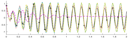
Adopt the framework of System 2. By pondering the computational time for running Scheme 5 and the match between System 1 and 2, we take . First, we test Schemes 1, 2, 4 and 5 by computing with . For any , . Since satisfies the quantum master equation (5) and is in the range of a few ten, we get the reference values of by calculating the explicit solution of (5). Second, we compute , the variance of . The reference values for the variance have been calculated by sampling times Scheme 2 with . It is worth pointing out that the maximal gap between the variances of produced by Schemes 1 and 2 with is of order of , while the maximal difference for Schemes 1 and 4 is .
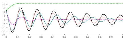
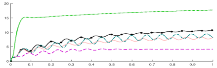
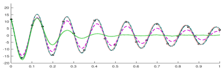
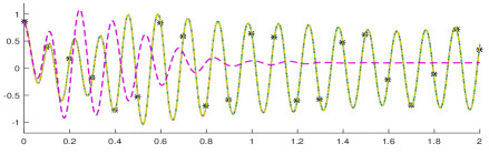
Figure 1 displays estimations of and obtained from sampling times Schemes 1, 2, 4 and 5 with step sizes equal to , and . Figure 1 shows that Schemes 1 and 2 reproduce very well the oscillatory behavior of . The first part of Table 1 provides the errors
where each numerical method is sampled times. Figure 1 together with Table 1, point out the superior accuracy of the exponential numerical methods Schemes 1 and 2 over Schemes 4 and 5. Furthermore, Scheme 5 has experienced serious difficulties in approximating System 2.
The second part of Table 1 presents the relative mean CPU time used for processing realizations of Schemes 1, 2, 4 and 5 with step size . Each has been estimated by averaging batches of numerical approximations. For a given , we report the ratio of the CPU time for each numerical method to the minimum of all CPU times, which corresponds to Scheme 4 with . Table 1 shows the advantages of solving (1) by means of the representation (9). In particular, the computational costs of Schemes 1, 2 and 4 are significantly lower than the one of Scheme 5. Moreover, the CPU time used by Scheme 2 is close to that of Scheme 1, thanks to Theorem 3.1.
Remark 10.
We examined the dimensions for which System 2 can be simulated running Scheme 1 on a current basic computer. To this end, we ran Scheme 1 with on a 3,3 GHz Intel Core i5 with 32 GB RAM. Recall that the dimension of the state space of System 2 is , and so here the density operators have elements. In the case where the matrix exponentials are calculated applying Padé approximants together with the scaling and squaring method, we could run Scheme 1 up to , and we were only able to compute the explicit solution of (5) if . Using Krylov subspace methods for the computation of matrix exponentials we ran Scheme 1 even with . Table 2 shows the dependence between and the time spent for ten integration steps of Scheme 1 with .
| Desktop 3,3 GHz Intel Core i5 with 32 GB RAM | 1.8 | 3.1 | 4.9 | 24.9 | 162.1 | 355.5 |
| Notebook 2,5 GHz Intel Core i7 with 16 GB RAM | 1.2 | 3.0 | 6.5 | 25.3 | 157.6 | 301.2 |
4.2 Direct detection
This subsection concerns with the numerical simulation of non-autonomous stochastic quantum master equations involving diffusion and jump terms. We study the following driven open quantum system, where a monochromatic laser light is applied to the field mode of the small quantum system under consideration.
System 3.
We take
acting upon , and so the small quantum system is driven by a coherent field of amplitude , frequency and phase (see, e.g., [23]). A noiseless counter is determined by , and the channel represents the loss light in the direct detection, where is the fraction of the detected fluorescent light and (see, e.g., [8]). The interaction between the two level system and a thermal bath is described by , as well as the interaction of the field mode with an independent reservoir is modeled by and . Here,
As in Section 4.1, we choose and . Moreover, we consider a coherent field with amplitude , frequency and phase . The measurement strength is set to and the fraction of the detected fluorescent light has been assumed . Finally, we select and . The initial density operator is the mixed state described by (6) with , and .

| Scheme 1 | ||||||||||
|---|---|---|---|---|---|---|---|---|---|---|
| Scheme 2 | ||||||||||
| Scheme 3 | ||||||||||
| Scheme 4 | ||||||||||
| Scheme 1 | ||||||||||
| Scheme 2 | ||||||||||
| Scheme 3 | ||||||||||
| Scheme 4 | ||||||||||
| Scheme 1 | ||||||||||
| Scheme 2 | ||||||||||
| Scheme 3 | ||||||||||
| Scheme 4 |

System 4.
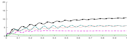
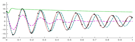
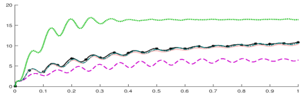
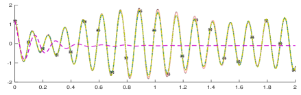
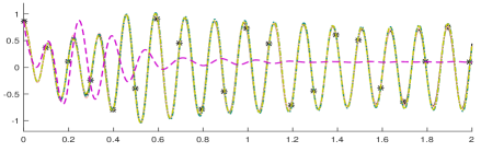
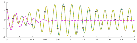
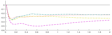
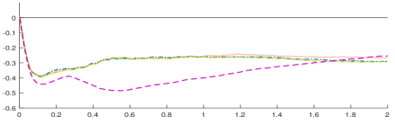
We simulate numerically System 4 with , which is a good approximation of System 3, by applying Schemes 1-4. In order to test the accuracy of Schemes 1-4, we compute and , where . The references values have been obtained by solving (5) via the ode45 MATLAB program, which is based on the Dormand-Prince method. Figure 2 shows estimations of and obtained from sampling times Schemes 1-4 with step sizes equal to , and . Table 3 provides the errors
and
as well as the relative mean CPU time used for processing 100 realizations of Schemes 1-4 with step size , which was calculated as in Table 1.
Figure 2 and Table 3 illustrate the good accuracy of Schemes 1, 2 and 3. In contrast to Scheme 4, Schemes 1-3 reproduce very well the oscillatory behavior as well as the amplitud modulation of the interference between the natural frequency of the small system and the driving coherent field.
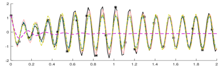
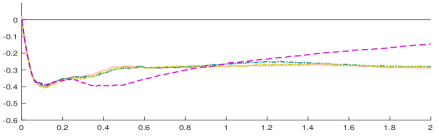
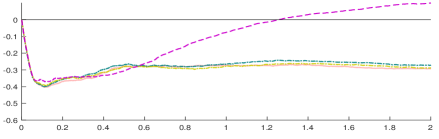
Now, we compute the Mandel -parameter:
| (25) |
which characterizes the departure of the number of photocounts from Poisson statistics (see, e.g., [8, 35, 36]). Figure 3 displays estimations of obtained from Schemes 1-4 with step sizes . Schemes 1-3 consistently show that takes negative values stabilizing around . These negative values indicate sub-Poissonian statistics that is an indicator of non-clasical effects, in a good agreement with the Physics of System 3. On the other hand, Scheme 4 change its behavior from sub-Poissonian statistics to Poissonian statistics as the step size decrease.
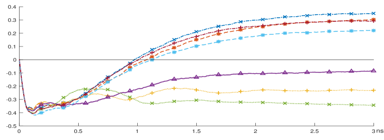
Finally, we study the behavior of System 3 for different frequencies of the monochromatic laser light, while keeping the other parameters unchanged. To this end, we simulate numerically System 4 with by using Scheme 1. Figure 4 presents the Mandel -parameter when , , , , , , ; we recall that the time is given in in nanoseconds. If is near the resonance frequency , then Figure 4 shows that takes negative values. In the other case, Schemes 1 predicts that varies from negative to positive values as the system evolves in time.

5 Proofs
5.1 Proof of Theorem 2.1
5.2 Proof of Theorem 3.1
Proof.
Since
simple algebraic manipulations yield and
Hence , and so
Hence
Using that for any matrix , we obtain the assertion of the theorem. ∎
5.3 Proof of Theorem 3.2
6 Conclusion
The numerical simulation of quantum measurement processes in continuous time, with mixed initial states, leads to solve stochastic quantum master equations (SQMEs for short). In a wide range of physical situations, the SQMEs are (or are approximated by) stiff stochastic differential equations in high-dimensional linear operator space. In order to overcome the difficulties arising in the direct numerical integration of SQMEs, we find a new representation of the solution to the jump-diffusion SQME by means of coupled non-linear stochastic Schrödinger equations. This has allowed us to design numerical methods for SQMEs based on new exponential schemes for jump-diffusion stochastic Schrödinger equations. Thus, we develop a set of numerical methods that accurately calculate stochastic density operators describing continuous measurements of quantum systems, even if we use a typical desktop computer and the Hilbert state space has dimension in the order of hundreds of thousand. We show the good performance of the new numerical integrators by simulating the continuous monitoring of two open quantum systems formed by a quantized electromagnetic field interacting with a two-level system, under the effect of the environment.
Acknowledgements
J.F. thanks the support of CONICYT grant CONICYT-PCHA/Doctorado Nacional/2013-21130792. C.M.M. was partially supported by FONDECYT Grant 1140411 and BASAL Grant PFB-03. C.M.M. is grateful to Alberto Barchielli and Matteo Gregoratti (Politecnico di Milano) for asking him about the numerical solution of stochastic quantum master equations, as well as for useful discussions on this topic. The authors thank the referees for their valuable comments and suggestions on the manuscript.
References
References
- [1] A. Abdulle, D. Cohen, G. Vilmart, and K. C. Zygalakis, High weak order methods for stochastic differential equations based on modified equations, SIAM J. Sci. Comput., 34 (2012), pp. A1800–A1823.
- [2] S. Agarwal, S. M. Hashemi Rafsanjani, and J. H. Eberly, Tavis-Cummings model beyond the rotating wave approximation: Quasidegenerate qubits, Phys. Rev. A, 85 (2012), p. 043815.
- [3] R. Alicki and K. Lendi, Quantum dynamical semigroups and applications, vol. 717 of Lecture Notes in Physics, Springer, Berlin, second edition ed., 2007.
- [4] H. Amini, M. Mirrahimi, and P. Rouchon, On stability of continuous-time quantum filters, in 2011 50th IEEE Conference on Decision and Control and European Control Conference, 2011, pp. 6242–6247.
- [5] S. Anmarkrud and A. Kværnø, Order conditions for stochastic Runge- Kutta methods preserving quadratic invariants of Stratonovich SDEs, J. Comput. Appl. Math., 316 (2017), pp. 40–46.
- [6] A. Barchielli and V. P. Belavkin, Measurements continuous in time and a posteriori states in quantum mechanics, J. Phys. A, 24 (1991), pp. 1495–1514.
- [7] A. Barchielli and M. Gregoratti, Quantum trajectories and measurements in continuous time: the diffusive case, vol. 782 of Lecture Notes in Physics, Springer, Berlin, 2009.
- [8] , Quantum measurements in continuous time, non-Markovian evolutions and feedback, Phil. Trans. R. Soc. A, 370 (2012), pp. 5364–5385.
- [9] A. Barchielli and A. Holevo, Constructing quantum measurement processes via classical stochastic calculus, Stochastic Process. Appl., 58 (1995), pp. 293–317.
- [10] A. Barchielli, C. Pellegrini, and F. Petruccione, Quantum trajectories: Memory and continuous observation, Phys. Rev A, 86 (2012), p. 063814.
- [11] D. Braak, Integrability of the Rabi model, Phys. Rev. Lett., 107 (2011), p. 100401.
- [12] P. Brémaud, Point processes and queues. Martingale dynamics, Springer Series in Statistics, Springer, New York-Berlin, 1981.
- [13] H. P. Breuer, U. Dorner, and F. Petruccione, Numerical integration methods for stochastic wave function equations, Comp. Phys. Commun., 132 (2000), pp. 30–43.
- [14] H. P. Breuer and F. Petruccione, The theory of open quantum systems, Oxford University Press, 2002.
- [15] H. J. Carmichael, Statistical Methods in Quantum Optics 2: Non-Classical Fields, Springer, 2008.
- [16] C. Chen and J. Hong, Symplectic Runge–Kutta semidiscretization for stochastic Schrödinger equation, SIAM Journal on Numerical Analysis, 54 (2016), pp. 2569–2593.
- [17] Y. S. Chow and H. Teicher, Probability theory: Independence, interchangeability, martingales, Springer-Verlag, New York, third edition ed., 1997.
- [18] K. L. Chung, A course in probability theory, Academic Press, San Diego, third edition ed., 2001.
- [19] J. Cui, J. Hong, Z. Liu, and W. Zhou, Stochastic symplectic and multi-symplectic methods for nonlinear Schrödinger equation with white noise dispersion, J. Comput. Phys., 342 (2017), pp. 267 – 285.
- [20] H. De la Cruz, R. J. Biscay, J. C. Jimenez, and F. Carbonell, Local linearization-Runge-Kutta methods: A class of A-stable explicit integrators for dynamical systems, Math. Comput. Modelling, 57 (2013), pp. 720–740.
- [21] A. C. Doherty, S. Habib, K. Jacobs, H. Mabuchi, and S. M. Tan, Quantum feedback control and classical control theory, Phys. Rev. A, 62 (2000), p. 012105.
- [22] E. Gallopoulos and Y. Saad, Efficient solution of parabolic equations by krylov approximation methods, SIAM J. Sci. Statist. Comput., 13 (1992), pp. 1236–1264.
- [23] J. Gambetta, A. Blais, M. Boissonneault, A. A. Houck, D. I. Schuster, and S. M. Girvin, Quantum trajectory approach to circuit QED: Quantum jumps and the Zeno effect, Phys. Rev. A, 77 (2008), p. 012112.
- [24] C. Graham and D. Talay, Stochastic simulation and Monte Carlo methods. Mathematical foundations of stochastic simulation, vol. 68, Springer, Heidelberg, 2013.
- [25] S. Haroche and J. M. Raimond, Exploring the Quantum: Atoms, Cavities, and Photons, Oxford University Press, 2006.
- [26] N. J. Higham, The scaling and squaring method for the matrix exponential revisited, SIAM J. Matrix Anal. Appl., 26 (2005), pp. 1179–1193.
- [27] , The scaling and squaring method for the matrix exponential revisited, SIAM Rev., 51 (2009), pp. 747–764.
- [28] M. Hochbruck and C. Lubich, On Krylov subspace approximations to the matrix exponential operator, SIAM J. Numer. Anal., 34 (1997), pp. 1911–1925.
- [29] J. Hong, D. Xu, and P. Wang, Preservation of quadratic invariants of stochastic differential equations via Runge- Kutta methods, Appl. Numer. Math., 87 (2015), pp. 38 – 52.
- [30] J. Jacod, Calcul stochastique et problèmes de martingales, vol. 714 of Lecture Notes in Mathematics, Springer, Berlin, 1979.
- [31] J. Jacod and P. Protter, Quelques remarques sur un nouveau type d’q́uations différentielles stochastiques, in Seminar on Probability XVI, vol. 920 of Lecture Notes in Math., Springer, Berlin-New York, 1982, pp. 447–458.
- [32] S. Jiang, L. Wang, and J. Hong, Stochastic multi-symplectic integrator for stochastic nonlinear Schrödinger equation, Commun. Comput. Phys., 14 (2013), pp. 393–411.
- [33] P. E. Kloeden and E. Platen, Numerical solution of stochastic differential equations, Springer, Berlin, 1992.
- [34] K. Kobayashi, Stochastic calculus for a time-changed semimartingale and the associated stochastic differential equations, J. Theoret. Probab., 24 (2011), pp. 789–820.
- [35] R. Loudon, The Quantum Theory of Light, Oxford University Press, Oxford, third edition ed., 2000.
- [36] L. Mandel and E. Wolf, Optical Coherence and Quantum Optics, Cambridge University Press, Cambridge, 1995.
- [37] G. N. Milstein and M. V. Tretyakov, Stochastic numerics for mathematical physics, Springer-Verlag, Berlin, 2004.
- [38] M. Mirrahimi and R. V. Handel, Stabilizing feedback controls for quantum systems, SIAM J. Control Optim., 46 (2007), pp. 445–467.
- [39] C. B. Moler and C. F. Van Loan, Nineteen dubious ways to compute the exponential of a matrix, twenty-five years later, SIAM Rev., 45 (2003), pp. 3–49.
- [40] C. Mora, Numerical solution of conservative finite-dimensional stochastic Schrödinger equations, Ann. Appl. Probab., 15 (2005), pp. 2144–2171.
- [41] C. M. Mora, Numerical simulation of stochastic evolution equations associated to quantum Markov semigroups, Math. Comp., 73 (2004), pp. 1393–1415.
- [42] , Heisenberg evolution of quantum observables represented by unbounded operators, J. Funct. Anal., 255 (2008), pp. 3249–3273.
- [43] , Regularity of solutions to quantum master equations: a stochastic approach, Ann. Probab., 41 (2013), pp. 1978–2012.
- [44] C. M. Mora, H. A. Mardones, J. C. Jimenez, M. Selva, and R. Biscay, A stable numerical scheme for stochastic differential equations with multiplicative noise, SIAM J. Numer. Anal., 55 (2017), pp. 1614–1649.
- [45] T. Niemczyk and et al., Circuit quantum electrodynamics in the ultrastrong-coupling regime, Nature Phys., 6 (2010), pp. 772–776.
- [46] C. Pellegrini, Existence, uniqueness and approximation of the jump-type stochastic Schrödinger equation for two-level systems, Stochastic Process. Appl., 120 (2010), pp. 1722–1747.
- [47] , Markov chains approximation of jump-diffusion stochastic master equations, Ann. Inst. H. Poincar Probab. Statist., 46 (2010), pp. 924–948.
- [48] I. C. Percival, Quantum state diffusion, Cambridge University Press, 1998.
- [49] M. B. Plenio and P. L. Knight, The quantum-jump approach to dissipative dynamics in quantum optics, Rev. Mod. Phys., 70 (1998), pp. 101–144.
- [50] P. E. Protter, Stochastic integration and differential equations, Springer-Verlag, Berlin, 2005.
- [51] P. Rouchon and J. F. Ralph, Efficient quantum filtering for quantum feedback control, Phys. Rev. A, 91 (2015), p. 012118.
- [52] M. Sarovar, C. Ahn, K. Jacobs, and G. J. Milburn, Practical scheme for error control using feedback, Phys. Rev. A, 69 (2004), p. 052324.
- [53] R. Schack, T. A. Brun, and I. C. Percival, Quantum state diffusion, localization and computation, J. Phys. A: Math. Gen., 28 (1995), pp. 5401–5413.
- [54] A. Shabani, J. Roden, and K. B. Whaley, Continuous measurement of a non-Markovian open quantum system, Phys. Rev. Lett., 112 (2014), p. 113601.
- [55] C. Van Loan, Computing integrals involving the matrix exponential, IEEE Trans. Automat. Control, 23 (1978), pp. 395–404.
- [56] H. Wang and Q. Ye, Error bounds for the Krylov subspace methods for computations of matrix exponentials, Preprint, arXiv:1603.07358v1 (2016).
- [57] H. Wiseman and G. J. Milburn, Quantum theory of optical feedback via homodyne detection, Phys. Rev. Lett., 70 (1993), pp. 548–551.
- [58] H. M. Wiseman and G. J. Milburn, Quantum measurement and control, Cambridge University Press,, 2009.
- [59] Z.-L. Xiang, S. Ashhab, J. Q. You, and F. Nori, Hybrid quantum circuits: Superconducting circuits interacting with other quantum systems, Rev. Mod. Phys., 85 (2013), p. 623.