SEAR: A Polynomial-Time Multi-Robot Path Planning Algorithm with Expected Constant-Factor Optimality Guarantee

Abstract

We study the labeled multi-robot path planning problem in continuous 2D and 3D domains in the absence of obstacles where robots must not collide with each other.

For an arbitrary number of robots in arbitrary initial and goal arrangements, we derive a polynomial time, complete algorithm that produces solutions with constant-factor optimality guarantees on both makespan and distance optimality, in expectation, under the assumption that the robot labels are uniformly randomly distributed.

Our algorithm only requires a small constant factor expansion of the initial and goal configuration footprints for solving the problem, i.e., the problem can be solved in a fairly small bounded region.

Beside theoretical guarantees, we present a thorough computational evaluation of the proposed solution. In addition to the baseline implementation, adapting an effective (but non-polynomial time) routing subroutine, we also provide a highly efficient implementation that quickly computes near-optimal solutions. Hardware experiments on the microMVP platform composed of non-holonomic robots confirms the practical applicability of our algorithmic pipeline.

I Introduction

In a labeled multi-robot path planning (MPP) problem, we are to move multiple rigid bodies (e.g., vehicles, mobile robots, quadcopters) from an initial configuration to a goal configuration in a collision-free manner. As a key sub-problem in many multi-robot applications, fast, optimal, and practical resolution to MPP are actively sought after. On the other hand, MPP, in its many forms, have been shown to be computationally hard [1, 2, 3, 4]. Due to the high computational complexity of MPP, there has been a lack of complete algorithms that provide concurrent guarantees on computational efficiency and solution optimality.

(a) Initial configuration	(b) Expand	(c) Assign
(d) Route	(e) Contract	(f) Goal configuration

Figure 1: Illustration of the expand-assign-route part of the (SEAR) pipeline. (a) the initial configuration. (a)$\to$(b) expansion to create space for moving the robots around. (b)$\to$(c) matching and snapping the robots onto a grid structure. (c)$\to$(d) routing the robots on graphs. (d)$\to$(e)$\to$(f) the contraction step, which is the reverse of the expand-assign steps. (f) the goal configuration.

In this paper, we take initial steps to fill this long-standing optimality-efficiency gap in labeled multi-robot path planning in continuous domains, without the presence of obstacles. We denote this version of the MPP problem as CMPP. Through the shift-expand-assign-route (SEAR) solution pipeline and the adaptation of a proper discrete robot routing algorithm [5], we derive a first polynomial time algorithm for solving CMPP in 2 or 3 dimensions that guarantees constant-factor solution optimality on both makespan (i.e., time to complete the reconfiguration task) and total distance (i.e., the sum of distances traveled by all robots), in expectation. For both initial and goal configurations, the robots may be located arbitrarily close to each other.

This work brings forth two main contributions. First, we introduce a novel pipeline, SEAR, for solving CMPP in an obstacle-free setting with very high robot density. With a proper discrete routing algorithm, we show that SEAR comes with strong theoretical guarantees on both computational time and solution optimality, which significantly improves over the state-of-the-art, e.g., [6]. Secondly, we have developed practical implementations of multiple SEAR-based algorithms, including highly efficient (but non-polynomial time) and near-optimal ones. As demonstrated through extensive simulation studies, SEAR can readily tackle problem instances with a thousand densely packed robots. We further demonstrate that SEAR can be applied to real multi-robot systems with differential constraints.

Related work. Variations of the multi-robot path planning problem have been actively studied for decades [7, 8, 9, 10, 11, 12, 13, 14, 15, 16, 17]. MPP finds applications in a diverse array of areas including assembly [18], evacuation [19], formation [20, 21], localization [22], microdroplet manipulation [23], object transportation [24], search and rescue [25], and human robot interaction [26], to list a few. Methods for resolving MPP can be centralized, where a central planner dictates the motion of all moving robots, or decentralized, where the moving robots make individual decisions [10, 27, 28]. Given the focus of the paper, our review of related literature focuses on centralized methods.

In a centralized planner, with full access to the system state, global planning and control can be readily enforced to drive operational efficiency. Methods in this domain may be further classified as coupled, decoupled, or a mixture of the two. Coupled methods treat all robots as a composite robot residing in $\mathcal{C}=\mathcal{C}^{1}\times\ldots\times\mathcal{C}^{n}$, where $\mathcal{C}^{i}$ is the configuration space of a single robot [29] and subsequently the problem is subjected to standard single robot planning methods [30, 31], such as A* in discrete domains [32] and sampling-based methods in continuous domains [33]. However, similar to high dimensional single robot problems [34], MPP is strongly NP-hard even for discs in simple polygons [1]. The hardness of the problem extends to the unlabeled case [3] although complete and optimal algorithms for practical scenarios have been developed [35, 13, 36, 14].

In contrast, decoupled methods first compute a path for each individual robot while ignoring all other robots. Interactions between paths are only considered a posteriori. The delayed coupling allows more robots to be simultaneously considered but may induce the loss of completeness [37]. One can however achieve completeness using optimal decoupling [38]. The classical approach in decoupling is through prioritization, in which an order is forced upon the robots [7], potentially significantly affect the solution quality[39], though remedy is possible to some extent [40]. Sometimes the priority may be imposed on the fly, which involves plan-merging and deadlock detection [41]. Often, priority is used in conjunction with velocity tuning, which iteratively decides the velocity of lower priority robots [42].

In the past decade, significant progress has been made on optimally solving (labeled) MPP problems in discrete settings, in particular on discrete (graph-base) environments. Here, the feasibility problem is solvable in $O(|V|^{3})$ time, in which $|V|$ is the number of vertices of the graph on which the robots reside [43, 44, 45]. Optimal MPP  remains computationally intractable in a graph-theoretic setting [46, 4], but the complexity has dropped from PSPACE-hard to NP-complete in many cases. On the algorithmic side, decoupling-based heuristics continue to prove to be useful [11, 15, 47]. Beyond decoupling, other ideas have also been explored, often through reduction to other problems [48, 49, 50].

Organization. The rest of this paper is structured as follows. In Section II, we state the problem setting. In Section III, after establishing the lower bound on achievable solution optimality, we introduce the SEAR at a high level. In Section IV, we describe the SEAR framework in full detail and provide a theoretical analysis of its key properties. In Section V, we evaluate the performance of algorithms explained in this paper. We conclude the paper in Section VI.

II Problem Formulation

Consider an obstacle-free $k$ dimensional environment ($k=2$ or $k=3$) and a set of $n$ labeled spherical (discs for 2D) robots with uniform radius $r$. The robots move with speed $\|v\|\in[0,1]$. For a robot $i$, let $x_{i}\in\mathbb{R}^{k}$ be its center; a joint configuration for all robot is then $X=(x_{1},\dots,x_{n})\in\mathbb{R}^{kn}$. Let $\|x_{i}-x_{j}\|$ be the Euclidean distance between $x_{i}$ and $x_{j}$, $1\leq i<j\leq n$, collision avoidance requires $\|x_{i}-x_{j}\|>2r$. Suppose the initial and goal configurations of the robots are $X^{I}$ and $X^{G}$, respectively, so that each robot $i$ is assigned an initial configuration $x_{i}^{I}$ and a goal configuration $x_{i}^{G}$. Denoting the set of all non-negative real numbers as $\mathbb{R}_{\geq 0}$, a plan is a function $\mathcal{P}:\mathbb{R}_{\geq 0}\to\mathbb{R}^{kn},t\mapsto X^{t}$ where for all $1\leq i\leq n,t,\varepsilon\in\mathbb{R}_{\geq 0}$, $\|x_{i}^{t}-x_{i}^{t+\varepsilon}\|\leq\varepsilon$. The continuous MPP instance studied in this paper is defined as follows.

Problem 1.

Continuous Multi-Robot Path Planning (CMPP). Given $X^{I},X^{G}$, find a plan $\mathcal{P}$ with $\mathcal{P}(0)=X^{I}$, and $\mathcal{P}(t)=X^{G}$ for all $t\geq T$.

We would like to find solutions with optimality assurance, according to the following objectives: 1) min-makespan: minimize the required time to finish the task, i.e. $T$; 2) min-total-distance: minimize the cumulative distance traveled by all robots. In particular, we are interested in situations where $X^{I}$ and $X^{G}$ are very dense. Therefore, we assume both $X^{I}$ and $X^{G}$ are bounded by orthotopes (a term generalizing and encompassing rectangles and cuboids) with volume linear to the total volume of robots, i.e., the volume of bounding orthotopes is $\Theta(nr^{k})$.

The probability of a particular $X^{I}$ (and $X^{G}$) occurring is assigned as follows. First, a collision free unlabeled configuration is fixed, for which a probability is difficult to assign. Instead, we assume that any labeling of the fixed unlabeled configuration has equal probability, i.e., each $X^{I}$ (and $X^{G}$) has a probability of $1/n!$, which allows us to avoid arguing about continuous probability spaces.

Figure 2: An illustration of CMPP when $n=3$ and $k=2$. The dashed circles are the bounding circles $c^{I}$ and $c^{G}$ with radii $r^{I}$ and $r^{G}$, respectively. In this case, $r_{b}=r^{G}$. The blue and red discs show the initial and goal configurations of the robots.

In the following sections, most illustrations and explanations assume $k=2$. Our results and proofs work for $k=3$. For developing the results, we introduce some additional notations. Given $X^{I}$ (resp., $X^{G}$), let $c^{I}$ (resp., $c^{G}$) centered at $o^{I}$ (resp., $o^{G}$) be the smallest bounding circle that encloses all $n$ robots. I.e., let the radius of $c^{I}$ (resp., $c^{G})$ be $r^{I}$ (resp., $r^{G}$), then for all $1\leq i\leq n$, $\|o^{I}-x_{i}^{I}\|\leq r^{I}-r$ (resp., $\|o^{G}-x_{i}^{G}\|\leq r^{G}-r$). We will use $r_{b}=\max\{r^{I},r^{G}\}$ and $d=\|o^{I}-o^{G}\|$ to state our optimality results. An illustrative CMPP instance with additional notations is given in Fig. 2.

III Main Results

III-A Lower Bounds on Optimality

In this sub-section, we establish lower bounds on the achievable optimality for CMPP. Since interchanging $X^{I}$ and $X^{G}$ does not affect optimality lower bounds, without loss of generality we make following assumptions: 1) $r_{b}=r^{G}\geq r^{I}$; 2) $X^{I}$ is fixed, while the labeling of $X^{G}$ is by an arbitrary permutation of $\{1,\ldots,n\}$.

Lemma III.1.

For any robot $1\leq i\leq n$, the probability that $\|x_{i}^{I}-x_{i}^{G}\|=o(r_{b})$ is less than or equal to $\frac{1}{4}$.

Proof.

Figure 3: Bounding rectangle of $X^{G}$ and the shaded area defined by $x_{i}^{I}$.

We will demonstrate the number of goal configurations with distance $o(r_{b})$ to $x_{i}^{I}$ is less than or equal to $\frac{n}{4}$.

Recall the assumption that $X^{I}$ and $X^{G}$ are bounded by orthotopes. As shown in Fig. 3, when $k=2$, the side lengths of the bounding rectangle of $X^{G}$ is denoted as $a$ and $b$. Without loss of generality, we assume $a\geq b$. The assumptions we made indicate that $a=\Theta(r^{G})=\Theta(r_{b})$, and $ab=\Theta(nr^{2})$. Now, consider a rectangle (the shaded area in Fig. 3) centered at the projection of $x_{i}^{I}$ on the longer central axis of rectangle $ab$, with side lengths $b$ and $c=\frac{n\pi r^{2}}{4b}$. Since $bc=\frac{n\pi r^{2}}{4}=\Theta(nr^{2})$, we deduce that $c=\Theta(a)=\Theta(r_{b})$, and the number of goal configurations fully contained in rectangle $bc$ is at most $\frac{n\pi r^{2}}{4}/\pi r^{2}=\frac{n}{4}$. Therefore, for an arbitrary labeling in $X^{G}$, the probability of $x_{i}^{G}$ to be fully contained in rectangle $bc$ is at most $\frac{1}{4}$, which covers all the cases that $\|x_{i}^{I}-x_{i}^{G}\|\leq\frac{c}{2}-r=\Theta(r_{b})-r$. Since $\pi r_{b}^{2}\geq n\pi r^{2}$, $\Theta(r_{b})-r=\Theta(r_{b})$. Thus, the probability that $\|x_{i}^{I}-x_{i}^{G}\|=o(r_{b})$ is less than or equal to $\frac{1}{4}$.

A similar approach can be applied to the case when $k=3$. The dimension of the bounding orthotope of $X^{G}$ is then denoted as $a\times b\times d$ ($a\geq b$, $a\geq d$), and the area around $x_{i}^{I}$ is defined as $c\times b\times d$, where $c=\frac{3}{16}\frac{n\pi r^{3}}{bd}$. Details are omitted due to the lack of space. ∎

We can then reason about optimality lower bounds of CMPP  based on the $n!$ problem instances generated by all the permutations of labeling in $X^{G}$.

Lemma III.2.

The fraction of problem instances with $o(r_{b})$ optimal makespan is at most $(\frac{1}{2})^{\frac{n}{2}}$.

Proof.

Note that an $o(r_{b})$ min-makespan requires $\|x_{i}^{I}-x_{i}^{G}\|=o(r_{b})$ to hold for all $1\leq i\leq n$. By Lemma III.1, for robot $1$, the probability that $\|x_{1}^{I}-x_{1}^{G}\|=o(r_{b})$ is at most $\frac{1}{4}$. Then, given that the assignments of goal configurations of different robots may be dependent, the probability that $\|x_{2}^{I}-x_{2}^{G}\|=o(r_{b})$ is at most $\frac{n/4}{n-1}$. Reasoning over the first $\frac{n}{2}$ robots, the probability that $\|x_{i}^{I}-x_{i}^{G}\|=o(r_{b})$ holds for all $1\leq i\leq\frac{n}{2}$ is at most $(\frac{1}{2})^{\frac{n}{2}}$. ∎

Lemma III.3.

The average optimal total travel distance of all the $n!$ instances is $\Omega(nr_{b})$.

Proof.

Denote $x_{ij}^{G}$ as the goal configuration of robot $j$ in problem instance $i$, the sum of optimal total travel distances of all the $n!$ instances is at least $\sum_{i=1}^{n!}\sum_{j=1}^{n}\|x_{j}^{I}-x_{ij}^{G}\|=\sum_{j=1}^{n}\sum_{i=1}^{n!}\|x_{j}^{I}-x_{ij}^{G}\|\geq\frac{3}{4}n!\sum_{j=1}^{n}\Theta(r_{b})=n!\,\Theta(nr_{b})$. Thus, the average optimal total travel distance is $\Omega(nr_{b})$. ∎

Taking $d$ into consideration, the optimality lower bounds on CMPP are fully established by the following lemma.

Lemma III.4.

For obstacle-free CMPP with an arbitrary permutation of robot labeling in $X^{I}$ and $X^{G}$, the lower bound of makespan is $\Omega(r_{b}+d)$, in expectation; the lower bound of total travel distance is $\Omega(n(r_{b}+d))$, in expectation.

Proof.

This Lemma extends the results from Lemma III.2 and Lemma III.3 by covering the case when $d=\omega(r_{b})$: each robot must travel a distance of at least $d-2r_{b}=\Theta(d)$. ∎

III-B SEAR and Upper Bounds on Optimality

The SEAR pipeline, as partially illustrated in Fig. 1, is outlined in Alg. 1. It contains four essential steps: (i) shift, (ii) expand, (iii) assign, and (iv) route. At the start of the pseudo code (line 1), the shift step moves the robots so that the centers of the bounding circles $c^{I}$ and $c^{G}$ coincide. Then, the expand and assign steps in lines 1-1 do the following: (i) expand the robots so that they are sufficiently apart, (ii) generate an underline grid $G(V,E)$, and (iii) perform an injective assignment from robot labels to $V$. This yields a discrete MPP sub-problem. Line 1 solves the new MPP problem. Line 1 then reverse the expand-assign to reach $X^{G}$. Note that the sub-plan for the contract step is generated together with the expand and assign steps. In particular, only a single grid $G$ is created. Because of this, we do not include contract as a unique step of the SEAR pipeline.

1 Shift: move all robots so that $o^{I}$ coincides with $o^{G}$

2 Expand: increase clearance between the robots

3 Construct a grid graph $G(V,E)$

4 Assign: move robots based on labeling $\{1,\ldots,n\}\xhookrightarrow{}V$

5 Route: solve the discrete MPP on $G$

6 Contract: reversed expand-assign steps

Algorithm 1 The SEAR Pipeline

We briefly analyze the optimality guarantee provided by SEAR; the details will follow in the next section. For an arbitrary robot, the shift step brings a distance cost of $d$. The expand step incurs a cost of $O(r_{b})$ and the assign step a cost of $O(r)$. This suggests that the contract step also incurs a cost of $O(r_{b}+r)=O(r_{b})$. The route step, using the algorithm introduced in [5], incurs a cost of $O(r_{b})$ as well. Adding everything together, the distance traveled by a single robot is $O(r_{b}+d)$. Since the SEAR pipeline solve the problem for all robots simultaneously, the makespan is $O(r_{b}+d)$ and the total distance is $O(n(r_{b}+d))$. In viewing Lemma III.4, we summarize the section with the following theorem, to be fully proved in the next section.

Theorem III.1.

For obstacle-free CMPP with an arbitrary permutation of robot labeling in $X^{I}$ and $X^{G}$, a SEAR-based algorithm can compute constant-factor optimal solutions for both makespan and total traveled distance, in expectation.

Remark.

Between the two objectives, makespan and total distance, our guarantee on makespan is stronger. For a problem $p_{i}$, let its minimum possible makespan be $t_{\min}(p_{i})$ and let the computed solution have makespan $t_{a}(p_{i})$, we in fact establish that the quantity $\sum_{i}\frac{t_{a}(p_{i})}{t_{\min}(p_{i})}$ is a constant.

IV The SEAR Pipeline in Detail

IV-A Shifting the Configuration Center

Lemma III.4 indicates that solving part of the problem with makespan $O(d)$ will not break the constant factor optimality guarantee. Therefore, the SEAR pipeline starts with a shift step that translates the robots without changing their relative positions, so that $o^{I}$ is moved to $o^{G}$ (see Fig. 4). During the process, the path travelled by robot $i$ is a straight line starts at $x_{i}^{I}$ and follows vector $\overrightarrow{o^{I}o^{G}}$. Since the workspace is free of obstacles, the shift step is always feasible and yields an updated CMPP with $d=0$. This process incurs exactly $d$ makespan and $nd$ total travel distance. The computational complexity is $O(n)$.

Figure 4: An illustration of shift step for the scenario in Fig. 2.

Without loss of generality, in the remaining part of this section, we assume $o^{I}=o^{G}$, and $d=0$.

IV-B Expand and Assign

We then apply expand and assign steps to both $X^{I}$ and $X^{G}$. The objective is to convert CMPP to a MPP on a grid graph $G=(V,E)$. The edge length of $G$ is dependent on $r$, the radius of robots. We illustrate the steps using $X^{I}$; the same procedure is applied to $X^{G}$ in the reverse order.

IV-B1 Expand

spread the robots so that there is enough clearance between them to move them onto $G$. For doing so, we use simple linear expansion as defined below.

Definition IV.1.

Linear Expansion. Denote $\lambda\geq 1$ as a scaling factor, each robot $i$ then moves along the direction of vector $\overrightarrow{o^{I}x_{i}^{I}}$ at maximum speed $1$, travels a distance $(\lambda-1)\|o^{I}-x_{i}^{I}\|$.

The value of $\lambda$, to be decided later, depends on grid property and also the placement of robots in $X^{I}$. Now, we first show that linear expansion is collision free.

Lemma IV.1.

Linear expansion is always collision-free.

Proof.

Because linear expansion with scaling factor $\lambda$ applies different travel distances to robots, we need to eliminate potential collisions between two moving robots, as well as between one moving robot and another stopped robot.

A pair of moving robots $i$ and $j$ always travel the same distance $t$ during time $[0,t]$ because they both move at the maximum speed $1$. As shown in Fig. 5(a), we denote $a=\|o^{I}-x_{i}^{I}\|,b=\|o^{I}-x_{j}^{I}\|$, and $\alpha=\angle~{}x_{i}^{I}o^{I}x_{j}^{I}$. The increased distance between $i$, $j$ during linear expansion is

$$\,(a+t)^{2}+(b+t)^{2}-2(a+t)(b+t)\cos\alpha-\|x_{i}^{I}-x_{j}^{I}\|$$

$$= \,2(1-\cos\alpha)(ta+tb+t^{2})\geq 0.$$

Since $\|x_{i}^{I}-x_{j}^{I}\|>2r$, two moving robots cannot collide.

The robots which are stopped earlier will not collide with any other robots afterwards. See Fig. 5(b), after robot $1$ stopped moving, the robots closer to $o^{I}$ (robot $2$, $3$, in the shaded area) are already stopped. As other robots (robot $4$, $5$, $6$, centered out of the shaded area) move away from the shaded area, the distance between any of them and robot $1$ monotonically increases. So they will not collide with robot $1$ in the future. ∎

(a)		(b)

Figure 5: Linear expansion. (a) Any two moving robots are collision-free. (b) The robots stopped will not collide with any other robot afterwards.

Corollary IV.1.

The distance between the center of any two robots after linear expansion is scaled up by a factor of $\lambda$.

Proof.

See Fig. 5(a), assume $x_{i}^{V},x_{j}^{V}$ are the configurations of robot $i,j$ after linear expansion, respectively. Because $\lambda=\|o^{I}-x_{i}^{V}\|/\|o^{I}-x_{i}^{I}\|=\|o^{I}-x_{j}^{V}\|/\|o^{I}-x_{j}^{I}\|$, $\lambda=\|x_{i}^{V}-x_{j}^{V}\|/\|x_{i}^{I}-x_{j}^{I}\|$. ∎

During linear expansion, because the travel distance of a robot is at most $(\lambda-1)(r_{b}-r)$, the makespan is $O(\lambda r_{b})$ and the total travel distance is $O(n\lambda r_{b})$.

Remark.

Depending on the specific problem instance, expansion could be achieved through multiple ways, as long as the robots move in a collision-free manner. That is, expand can be done in a smarter way. However (intuitively and as we will show), linear expansion with a small constant $\lambda$ is sufficient for the SEAR analysis to carry through.

IV-B2 Assign

After expansion, we generate a regular grid graph $G$ in an area which covers all robots. Here, we use hexagonal grid for illustration due to its capability for accommodating high robot density and natural support for certain differential constraints [51]. In this case, to ensure the robots can move along edges in $G$ without collisions, the edge/side length $\ell$ should be greater than $(4/\sqrt{3})r$ [51]. We first establish the number of vertices in $G$ so that $G$ fully covers the expanded $X^{I}$ and $X^{G}$.

Lemma IV.2.

The number of vertices in $G$ is $O(\lambda^{k}r_{b}^{k}/\ell^{k})$.

Proof.

After linear expansion, the side length of the smallest bounding orthotope of all robots is not larger than $\lambda r_{b}$. If we construct $G$ in this area, then $|V|=O(\lambda^{k}r_{b}^{k}/\ell^{k})$. ∎

The next step is to place the robots on $V$. This is done by assign each robot to the nearest vertex, and execute straight line paths at the full speed $1$. For a given $X^{I}$, we define $d_{min}=\min_{1\leq i<j\leq n}\|x_{i}^{I}-x_{j}^{I}\|.$

Lemma IV.3.

When $\lambda\geq 2\ell/d_{min}$, the following statements holds: (i) the mapping between robot labels $\{1,\ldots,n\}$ and $V$ is injective; (ii) the assigned paths are collision-free.

Proof.

(i) When $\lambda\geq 2\ell/d_{min}$, Corollary IV.1 implies that after linear expansion, robots are located in non-overlapping circles with radius $\ell$ (see Fig. 6(a)). Hence, there must be at least one vertex in $V$ lands inside or on the border of each circle, which is assigned to the robot in the circle. This ensures the injective mapping between robot labels and $V$.

(ii) As it is shown in Fig 6(b), we denote the configurations of robot $i,j$ after expansion as $x_{i}^{V},x_{j}^{V}$, and the vertices assigned to the two robots as $v_{i}$, $v_{j}$, respectively. From (i), we deduce that $\|x_{i}^{V}-v_{i}\|\leq\ell,\|x_{i}^{V}-v_{j}\|\geq\ell$, and $\|x_{i}^{V}-x_{j}^{V}\|\geq 2\ell$. Since $\ell$ denote edge length in $G$, $\|v_{i}-v_{j}\|\geq\ell$. These inequations imply that the distance (the red dashed line) from $v_{j}$ to segment $x_{i}^{V}v_{i}$ is at least $(\sqrt{3}/2)\ell$. The above statements also holds for $v_{i}$ and $x_{j}^{V}v_{j}$. Thus, the shortest distance between segments $x_{i}^{V}v_{i}$ and $x_{j}^{V}v_{j}$ is $(\sqrt{3}/2)\ell>(\sqrt{3}/2)(4/\sqrt{3})r=2r$. No collisions between robot $i,j$. ∎

(a)		(b)

Figure 6: Assign. (a) The robots are in circles with radius $\ell$ which do not overlap. (b) No collision between the trajectories.

Denote $\varepsilon$ as a small positive real number, if we let $\ell=(4/\sqrt{3})r+\varepsilon$, then $2\ell/d_{min}\leq 2\ell/2r=4/\sqrt{3}+\varepsilon/2r$. In this case, it is safe to say that when $\lambda=4/\sqrt{3}+\varepsilon/2r$, the expand-assign can always be successfully performed. $\lambda$ can be smaller when $d_{min}$ is larger. The makespan for the whole expand-assign step is $O(r_{b})$, and the total travel distance is $O(nr_{b})$. In viewing Lemma IV.2, the computational time is $O(n|V|)$, with the dominating factor being matching the robots with their nearest vertices.

An alternative for the expand-assign step is to consider matching robot labels to $V$ as an unlabeled MPP problem in continuous domain. Because the makespan for expand-assign is already sufficient for achieving the desired optimality, we opt to keep the method fast and straightforward.

Remark.

In the actual implementation, we also added an extra step that “compacts” the MPP instance, which makes the initial and goal configurations on the graph $G$ more concentrated. The extra step, based largely on [35], does not impact the asymptotic performance of the SEAR pipeline but produces better constants.

IV-C Discrete Robot Routing

After applied expand and assign steps to both $X^{I}$ and $X^{G}$, a CMPP instance becomes a discrete MPP instance. Let the converted instance be $(G,V^{I},V^{G})$, i.e., $V^{I}=\{v_{1}^{I},\ldots,v_{n}^{I}\}$ and $V^{G}=\{v_{1}^{G},\ldots,v_{n}^{G}\}$ are the discrete initial and goal configurations of the robots on $G$. To solve the MPP instance with polynomial time complexity and constant factor optimality guarantee, we apply the SplitAndGroup (SAG) algorithm [5]. The algorithm is intended for a fully occupied graph, but is also directly applicable to sparse graphs: we may place “virtual robots” on empty vertices. For completeness, we provide a brief overview of SAG here.

SAG is a recursive algorithm that splits a MPP instance into smaller sub-problems in each level of recursive call. We demonstrate one recursion here as an illustration. As shown in Fig. 7(a), split partitions the part of grid it works on into two areas (left side with a blue shade and right side with a red shade) along the longer side of this grid. For each side, the algorithm finds all the robots currently in this side with goal vertices in the other side. Here in Fig. 7, the blue (resp. red) robots have goal vertices in blue (resp. red) shade. Then group moves every robot to the side where its goal vertex belongs to (see Fig. 7(b)). This results in two sub-problems (the left one and the right one), which could be treated by the next level of recursion call in parallel.

(a) Before		(b) After

Figure 7: Before and after one recursive call of SAG.

The grouping procedure depends on the robots being able to “swap” locations locally in constant time. On a hexagonal grid, swapping any two robots on a fully occupied figure-8 graph (Fig. 8) can be performed in constant time through an adaptation of the proof used in proving Lemma 1 of [5]. As a larger grid is partitioned into smaller figure-8 graphs, parallel swaps become possible. Let $G$ be bounded in a rectangle of size $m_{w}\times m_{h}$ in which $m_{w}$ and $m_{h}$ are the width and height of the rectangle, then the first iteration of SAG requires a robot incur a makespan of $O(m_{w}+m_{h})$ and this can be done in parallel for all robots. Recursively, the makespan upper bound of SAG (applied to our problem) is:

$$\begin{array}[]{ll}&\displaystyle O(m_{w}+m_{h})+O(\frac{m_{w}}{2}+m_{h})+O(\frac{m_{w}}{2}+\frac{m_{h}}{2})+\dots\\ =&\displaystyle O(m_{w}+m_{h})=O(\lambda r_{b})=O(r_{b}).\end{array}$$

The last equality is due to $\lambda$ being a small constant.

Figure 8: Figure-8 graphs in hexagonal grids and square grids.

SAG incurs $O(|V|^{3})=O((\lambda^{k}r_{b}^{k}/l^{k})^{3})=O((\lambda^{k}nr^{k}/l^{k})^{3})=O(n^{3})$ computational time.

IV-D Performance Analysis of SEAR

Summarizing the result from individual steps, for the general SEAR pipeline with the shift step, we conclude

Theorem IV.1.

For obstacle-free CMPP, SEAR computes solutions with $O(r_{b}+d)$ makespan and $O(n(r_{b}+d))$ total distance in $O(n^{3})$ computational time.

Theorem III.1 follows Lemma III.4 and Theorem IV.1.

IV-E Generalization to a 3 Dimensional Workspace

SEAR is ready to be generalized to a 3 dimensional workspace with some modifications to key parameters. The shift step can be applied to an arbitrary dimension. In the expand and assign steps, suppose a cube grid is used, the edge length $l$ should be at least $(4/\sqrt{2})r+\varepsilon$ to ensure that robots can move along edges without collisions. A scale factor $\lambda=4/\sqrt{2}+\varepsilon/2r$ is sufficient for assign to be collision-free. For any fixed dimension, the guarantee of the SAG algorithm continuous to hold [5]. With these modifications, Theorem IV.1 and Theorem III.1 holds for $k=3$.

V Evaluation

In this section, we provide evaluations of computational time and solution optimality of SEAR-based algorithms when $k=2$. A hardware experiment is also carried out to verify the support for differential constraints. In our implementation, beside the baseline SEAR with SAG, we also implemented an SEAR algorithm with the high quality (but non-polynomial-time) ILP solver from [50]. We denote SEAR with SAG as SEAR-SAG, and SEAR with ILP solver as SEAR-ILP. SEAR-ILP-$m$ indicates the usage of $m$-way split heuristics [50]. We use makespan as the key metric which also bounds the total distance and maximum distance. Additionally, instead of simply using the makespan value, which is less informative, we divide it by an underestimated minimum makespan $\max_{1\leq i\leq n}\|x_{i}^{I}-x_{i}^{G}\|$.

SEAR-SAG is implemented in Python. The SEAR-ILP implementation is partially based on the Java code from [50], which utilizes the Gurobi ILP solver [52]. Since the robot radius $r$ is relative, we fix $r=1$. To capture denseness of the setup, we introduce $2r+\delta$ as the minimum distance between two robots allowed when generating $X^{I}$ and $X^{G}$. The region where the robots may appear is limited to a circle of radius $1.5$ times the radius of the smallest circle that $n$ discs with radius $r+\delta/2$ could fit in [53]. The edge length of hexagonal grids is $\ell=4/\sqrt{3}$. The scaling factor $\lambda=\ell/(\delta/2+r)$. Our evaluation mainly focuses on $d=0$ since the shift step is straightforward. An example instance is provided in Fig. 9.

Figure 9: An example of a randomly generated CMPP with $n=10,\delta=0,d=0$. The left and right figure indicates $X^{I}$ and $X^{G}$, respectively. Part of the hexagonal graph generated by SEAR is rendered in the background.

Problem instances are generated by assiging arbitrary labeling to uniformly randomly sampled robot configurations in continuous space. For each set of parameters $(n,\delta,d)$, $10$ instances are attempted and the average is taken. A data point is only recorded if all 10 instances are completed successfully. All experiments were executed on a Intel^® Core^TM i7-6900K CPU with 32GB RAM at 2133MHz.

V-A SEAR-SAG

To observe the basic behavior of SEAR-SAG, we fix $\delta=d=0$ and evaluate SEAR-SAG on both hexagonal grids and square grids by increasing $n$. For square grids, $l=4/\sqrt{2},\lambda=2/(\delta/2+r)$. The result is in Fig. 10. From the computational time aspect (see Fig. 10 (a)), SEAR-SAG is able to solve problems with $1000$ robots within $800$ seconds. On the optimality side (see Fig. 10 (b)), because of the simple implementation and the dense setting, the optimality ratio of solutions generated by SEAR-SAG is relatively large. For example, the makespan for hexagonal grid is $75$ times the underestimated makespan when $n=20$. We can observe, however, that the ratio between the solution makespan and the underestimated makespan flattens out as $n$ grows, confirming the constant factor optimality property of SEAR.

We note that the guaranteed optimality of SEAR is in fact sub-linear with respect to the number of robots, which is clearly illustrated in Fig. 11. As we can observe, the makespan is proportional to the number of vertices on the longer side of the grid, which in turn is proportional to $\sqrt{n}$.

(a)		(b)

Figure 10: Computational time and optimality ratio of SEAR-SAG versus the number of robots.

Figure 11: Makespan of SEAR-SAG versus the number of vertices on the longer side of the grid.

V-B SEAR-SAG vs. SEAR-ILP

We then compare SEAR-SAG and SEAR-ILP on hexagonal grids. First we let $\delta=d=0$ and gradually increase $n$. The performance of the algorithms agrees with the expectation (see Fig. 12). SEAR-ILP guarantees the optimal solution on the MPP sub-problem. However, its running time grows quickly and becomes unstable. It cannot always solve a problem instance in $30$ minutes when $n>50$. Nevertheless, the split heuristic makes SEAR-ILP more applicable when $n$ is large. For example, the running time of SEAR-ILP with 4-way split is about the same as SEAR-SAG when $n=700$. Although SEAR-ILP with split heuristic can solve problems with hundreds of robots, when $n\geq 800$, only SEAR-SAG could finish due to its polynomial time complexity.

The makespan of solutions generated by SEAR-ILP is quite low and practical, since it always provides the optimal solution to MPP sub-problems. For instance, when $n=40$, the makespan of generated solutions is $4.93$ times the estimated value. The optimality of SEAR-ILP with split heuristics are also close to being optimal. When $n=500$, SEAR-ILP with 4-way split provides solutions with makespan $4.73$ times the underestimated value.

(a)		(b)

Figure 12: Performance of SEAR algorithms as $n$ varies.

To model different density of robots, we then fix $n=30,d=0$ and increase $\delta$. With a larger $\delta$, $\lambda$ could be smaller, which makes robots move less during linear scaling. Fig. 13 demonstrates the performance of the methods as $\delta$ goes from $0$ to $2.6$ (when $\delta\geq 8/\sqrt{3}-2\approx 2.62$, no expansion is required). Here, since $n$ and $|V|$ are not changed, the size of the MPP sub-problems remains the same. Thus the computational time of the algorithms stays static. On the other hand, the optimality ratio becomes lower as $\delta$ grows, due to the increasement of the underestimated makespan.

(a)		(b)

Figure 13: Performance of SEAR algorithms as $\delta$ varies.

For the last part of our experiment, we fix $n=30,\delta=0$ and change $d$. As we can observe in Fig.14, the solution becomes closer to optimal as $d$ increases, as expected.

(a)		(b)

Figure 14: Performance of SEAR algorithms as $d$ varies.

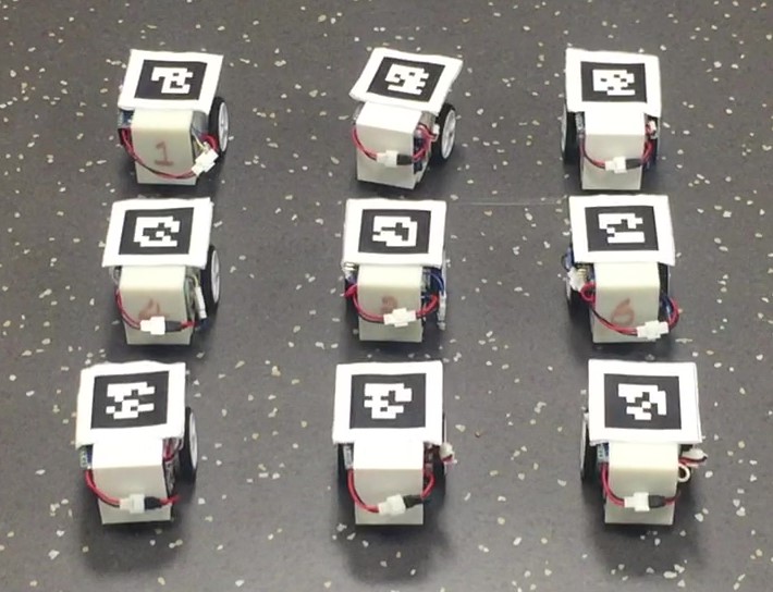
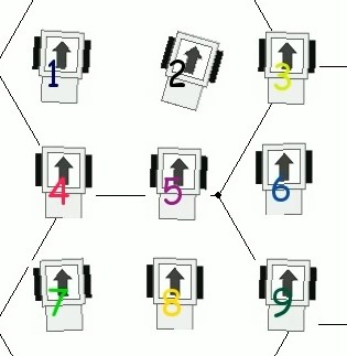
(a)	(b)

Figure 15: The hardware experimentation. (a) The paths generated by SEAR are executed by differential drive cars. (b) Part of a Python-based UI, which is used to monitor and control the vehicles.

Both software simulation and hardware experimentation of the proposed algorithms can be found in the video attachment. The hardware implementation (details in Fig. 15) is based on the microMVP platform [54].

VI Conclusion

In this paper, we proposed the SEAR solution pipeline for tackling continuous multi-robot path planning (CMPP) problem in the absence of obstacles. We show that SEAR-based algorithms provide strong theoretical guarantees. With an alternative sub-routine for the discrete MPP instance, SEAR also proves to be practical, as confirmed by simulation and hardware experiment.

The current iteration of the SEAR-based algorithms has focused on theoretical guarantees; many additional improvements are possible. For example, the expand and assign steps can be done in an adaptive manner that avoids uniform scaling, which should greatly boost the optimality of the resulting algorithm. Additionally, the current SEAR pipeline only provide ad-hoc support for robots differential constraints. In an extension to the current work, we plan to further improve the efficiency and optimality of SEAR and add generic support for robots with differential constraints including aerial vehicle swarms.

References

- [1] P. Spirakis and C. K. Yap, “Strong NP-hardness of moving many discs,” Information Processing Letters, vol. 19, no. 1, pp. 55–59, 1984.
- [2] J. E. Hopcroft, J. T. Schwartz, and M. Sharir, “On the complexity of motion planning for multiple independent objects; PSPACE-hardness of the “warehouseman’s problem”,” The International Journal of Robotics Research, vol. 3, no. 4, pp. 76–88, 1984.
- [3] K. Solovey and D. Halperin, “On the hardness of unlabeled multi-robot motion planning,” in Robotics: Science and Systems (RSS), 2015.
- [4] J. Yu, “Intractability of optimal multi-robot path planning on planar graphs,” IEEE Robotics and Automation Letters, vol. 1, no. 1, pp. 33–40, 2016.
- [5] ——, “Expected constant-factor optimal multi-robot path planning in well-connected environments,” in Multi-Robot and Multi-Agent Systems (MRS), 2017 International Symposium on. IEEE, 2017, pp. 48–55.
- [6] S. Tang and V. Kumar, “A complete algorithm for generating safe trajectories for multi-robot teams,” in Robotics Research. Springer, 2018, pp. 599–616.
- [7] M. A. Erdmann and T. Lozano-Pérez, “On multiple moving objects,” in Proceedings IEEE International Conference on Robotics & Automation, 1986, pp. 1419–1424.
- [8] S. M. LaValle and S. A. Hutchinson, “Optimal motion planning for multiple robots having independent goals,” IEEE Transactions on Robotics & Automation, vol. 14, no. 6, pp. 912–925, Dec. 1998.
- [9] Y. Guo and L. E. Parker, “A distributed and optimal motion planning approach for multiple mobile robots,” in Proceedings IEEE International Conference on Robotics & Automation, 2002, pp. 2612–2619.
- [10] J. van den Berg, M. C. Lin, and D. Manocha, “Reciprocal velocity obstacles for real-time multi-agent navigation,” in Proceedings IEEE International Conference on Robotics & Automation, 2008, pp. 1928–1935.
- [11] T. Standley and R. Korf, “Complete algorithms for cooperative pathfinding problems,” in Proceedings International Joint Conference on Artificial Intelligence, 2011, pp. 668–673.
- [12] K. Solovey and D. Halperin, “-color multi-robot motion planning,” in Proceedings Workshop on Algorithmic Foundations of Robotics, 2012.
- [13] M. Turpin, K. Mohta, N. Michael, and V. Kumar, “CAPT: Concurrent assignment and planning of trajectories for multiple robots,” International Journal of Robotics Research, vol. 33, no. 1, pp. 98–112, 2014.
- [14] K. Solovey, J. Yu, O. Zamir, and D. Halperin, “Motion planning for unlabeled discs with optimality guarantees,” in Robotics: Science and Systems, 2015.
- [15] G. Wagner and H. Choset, “Subdimensional expansion for multirobot path planning,” Artificial Intelligence, vol. 219, pp. 1–24, 2015.
- [16] L. Cohen, T. Uras, T. Kumar, H. Xu, N. Ayanian, and S. Koenig, “Improved bounded-suboptimal multi-agent path finding solvers,” in International Joint Conference on Artificial Intelligence, 2016.
- [17] B. Araki, J. Strang, S. Pohorecky, C. Qiu, T. Naegeli, and D. Rus, “Multi-robot path planning for a swarm of robots that can both fly and drive,” in IEEE Int. Conf. on Robotics and Automation (ICRA), 2017.
- [18] D. Halperin, J.-C. Latombe, and R. Wilson, “A general framework for assembly planning: The motion space approach,” Algorithmica, vol. 26, no. 3-4, pp. 577–601, 2000.
- [19] S. Rodriguez and N. M. Amato, “Behavior-based evacuation planning,” in Proceedings IEEE International Conference on Robotics & Automation, 2010, pp. 350–355.
- [20] S. Poduri and G. S. Sukhatme, “Constrained coverage for mobile sensor networks,” in Proceedings IEEE International Conference on Robotics & Automation, 2004.
- [21] B. Smith, M. Egerstedt, and A. Howard, “Automatic generation of persistent formations for multi-agent networks under range constraints,” ACM/Springer Mobile Networks and Applications Journal, vol. 14, no. 3, pp. 322–335, Jun. 2009.
- [22] D. Fox, W. Burgard, H. Kruppa, and S. Thrun, “A probabilistic approach to collaborative multi-robot localization,” Autonomous Robots, vol. 8, no. 3, pp. 325–344, Jun. 2000.
- [23] E. J. Griffith and S. Akella, “Coordinating multiple droplets in planar array digital microfluidic systems,” International Journal of Robotics Research, vol. 24, no. 11, pp. 933–949, 2005.
- [24] D. Rus, B. Donald, and J. Jennings, “Moving furniture with teams of autonomous robots,” in Proceedings IEEE/RSJ International Conference on Intelligent Robots & Systems, 1995, pp. 235–242.
- [25] J. S. Jennings, G. Whelan, and W. F. Evans, “Cooperative search and rescue with a team of mobile robots,” in Proceedings IEEE International Conference on Robotics & Automation, 1997.
- [26] R. A. Knepper and D. Rus, “Pedestrian-inspired sampling-based multi-robot collision avoidance,” in 2012 IEEE RO-MAN: The 21st IEEE International Symposium on Robot and Human Interactive Communication. IEEE, 2012, pp. 94–100.
- [27] J. Snape, J. van den Berg, S. J. Guy, and D. Manocha, “The hybrid reciprocal velocity obstacle,” IEEE Transactions on Robotics, vol. 27, no. 4, pp. 696–706, 2011.
- [28] S. Kim, S. J. Guy, K. Hillesland, B. Zafar, A. A.-A. Gutub, and D. Manocha, “Velocity-based modeling of physical interactions in dense crowds,” The Visual Computer, vol. 31, no. 5, pp. 541–555, 2015.
- [29] J. T. Schwartz and M. Sharir, “On the piano movers problem. ii. general techniques for computing topological properties of real algebraic manifolds,” Advances in applied Mathematics, vol. 4, no. 3, pp. 298–351, 1983.
- [30] J.-C. Latombe, Robot motion planning. Springer Science & Business Media, 2012, vol. 124.
- [31] S. M. LaValle, Planning Algorithms. Cambridge, U.K.: Cambridge University Press, 2006, also available at http://planning.cs.uiuc.edu/.
- [32] P. Hart, N. J. Nilsson, and B. Raphael, “A formal basis for the heuristic determination of minimum cost paths,” IEEE Transactions on Systems Science and Cybernetics, vol. 4, pp. 100–107, 1968.
- [33] K. Solovey, O. Salzman, and D. Halperin, “Finding a needle in an exponential haystack: Discrete RRT for exploration of implicit roadmaps in multi-robot motion planning,” in Proceedings Workshop on Algorithmic Foundations of Robotics, 2014.
- [34] J. H. Reif, “Complexity of the generalized mover’s problem.” DTIC Document, Tech. Rep., 1985.
- [35] J. Yu and S. M. LaValle, “Distance optimal formation control on graphs with a tight convergence time guarantee,” in Proceedings IEEE Conference on Decision & Control, 2012, pp. 4023–4028.
- [36] A. Adler, M. De Berg, D. Halperin, and K. Solovey, “Efficient multi-robot motion planning for unlabeled discs in simple polygons,” in Algorithmic Foundations of Robotics XI. Springer, 2015, pp. 1–17.
- [37] G. Sanchez and J.-C. Latombe, “Using a prm planner to compare centralized and decoupled planning for multi-robot systems,” in Robotics and Automation, 2002. Proceedings. ICRA’02. IEEE International Conference on, vol. 2. IEEE, 2002, pp. 2112–2119.
- [38] J. van den Berg, J. Snoeyink, M. Lin, and D. Manocha, “Centralized path planning for multiple robots: Optimal decoupling into sequential plans,” in Robotics: Science and Systems, 2009.
- [39] J. van den Berg and M. Overmars, “Prioritized motion planning for multiple robots,” in Proceedings IEEE/RSJ International Conference on Intelligent Robots & Systems, 2005.
- [40] M. Bennewitz, W. Burgard, and S. Thrun, “Finding and optimizing solvable priority schemes for decoupled path planning techniques for teams of mobile robots,” Robotics and autonomous systems, vol. 41, no. 2, pp. 89–99, 2002.
- [41] M. Saha and P. Isto, “Multi-robot motion planning by incremental coordination,” in 2006 IEEE/RSJ International Conference on Intelligent Robots and Systems. IEEE, 2006, pp. 5960–5963.
- [42] K. Kant and S. Zucker, “Towards efficient trajectory planning: The path velocity decomposition,” International Journal of Robotics Research, vol. 5, no. 3, pp. 72–89, 1986.
- [43] V. Auletta, A. Monti, M. Parente, and P. Persiano, “A linear-time algorithm for the feasbility of pebble motion on trees,” Algorithmica, vol. 23, pp. 223–245, 1999.
- [44] G. Goraly and R. Hassin, “Multi-color pebble motion on graph,” Algorithmica, vol. 58, pp. 610–636, 2010.
- [45] J. Yu, “A linear time algorithm for the feasibility of pebble motion on graphs,” arXiv:1301.2342, 2013.
- [46] O. Goldreich, “Finding the shortest move-sequence in the graph-generalized 15-puzzle is NP-hard,” 1984, laboratory for Computer Science, Massachusetts Institute of Technology, Unpublished manuscript.
- [47] E. Boyarski, A. Felner, R. Stern, G. Sharon, O. Betzalel, D. Tolpin, and E. Shimony, “Icbs: The improved conflict-based search algorithm for multi-agent pathfinding,” in Eighth Annual Symposium on Combinatorial Search, 2015.
- [48] P. Surynek, “Towards optimal cooperative path planning in hard setups through satisfiability solving,” in Proceedings 12th Pacific Rim International Conference on Artificial Intelligence, 2012.
- [49] E. Erdem, D. G. Kisa, U. Öztok, and P. Schueller, “A general formal framework for pathfinding problems with multiple agents.” in AAAI, 2013.
- [50] J. Yu and S. M. LaValle, “Optimal multi-robot path planning on graphs: Complete algorithms and effective heuristics,” IEEE Transactions on Robotics, vol. 32, no. 5, pp. 1163–1177, 2016.
- [51] J. Yu and D. Rus, “An effective algorithmic framework for near optimal multi-robot path planning,” in Robotics Research. Springer, 2018, pp. 495–511.
- [52] Gurobi Optimization, Inc., “Gurobi optimizer reference manual,” 2014. [Online]. Available: http://www.gurobi.com
- [53] E. Specht, The best known packings of equal circles in a circle (complete up to N = 2600), Nov. 2016. [Online]. Available: http://hydra.nat.uni-magdeburg.de/packing/cci/cci.html
- [54] J. Yu, S. D. Han, W. N. Tang, and D. Rus, “A portable, 3D-printing enabled multi-vehicle platform for robotics research and education,” in IEEE International Conference on Robotics and Automation, 2017.