Transverse Magnetic Susceptibility of a Frustrated Spin-$\frac{1}{2}$ $J_{1}$–$J_{2}$–$J_{1}^{\perp}$ Heisenberg Antiferromagnet on a Bilayer Honeycomb Lattice

Abstract

We use the coupled cluster method (CCM) to study a frustrated spin-$\frac{1}{2}$ $J_{1}$–$J_{2}$–$J_{1}^{\perp}$ Heisenberg antiferromagnet on a bilayer honeycomb lattice with $AA$ stacking. Both nearest-neighbor (NN) and frustrating next-nearest-neighbor antiferromagnetic (AFM) exchange interactions are present in each layer, with respective exchange coupling constants $J_{1}>0$ and $J_{2}\equiv\kappa J_{1}>0$. The two layers are coupled with NN AFM exchanges with coupling strength $J_{1}^{\perp}\equiv\delta J_{1}>0$. We calculate to high orders of approximation within the CCM the zero-field transverse magnetic susceptibility $\chi$ in the Néel phase. We thus obtain an accurate estimate of the full boundary of the Néel phase in the $\kappa\delta$ plane for the zero-temperature quantum phase diagram. We demonstrate explicitly that the phase boundary derived from $\chi$ is fully consistent with that obtained from the vanishing of the Néel magnetic order parameter. We thus conclude that at all points along the Néel phase boundary quasiclassical magnetic order gives way to a nonclassical paramagnetic phase with a nonzero energy gap. The Néel phase boundary exhibits a marked reentrant behavior, which we discuss in detail.

1 INTRODUCTION

The study of the zero-temperature $(T=0)$ quantum phase transitions (QPTs) that can occur in strongly-interacting quantum many-body systems has become a field of huge current interest [1, 2] in condensed matter physics. Quantum spin-lattice models have become a particularly interesting test-bed in this context since they exhibit such a wide variety of phases at $T=0$, ranging from (partially) ordered quasiclassical states with magnetic long-range order (LRO) to such nonclassical states as those with valence-bond crystalline (VBC) order and various quantum spin liquid (QSL) phases. All such quantum magnets basically comprise an extended regular periodic lattice in $d$ dimensions of a specified form, on each of the $(N\rightarrow\infty)$ sites of which is situated a magnetic ion with spin quantum number $s$.

A particularly important class of such spin-lattice models comprises those in which the spins interact only via a pairwise term in the Hamiltonian of the isotropic Heisenberg form $J_{ij}\mathbf{s}_{i}\cdot\mathbf{s}_{j}$, between spins at lattice sites $i$ and $j$. If we restrict the exchange couplings $J_{ij}$ to be only between nearest-neighbor (NN) pairs of sites on the lattice, and further restrict all NN pairs to be magnetically equivalent, so that each pair feels the same exchange coupling $J_{1}$, then the only relevant parameter (for a given lattice type and for specified values of $d$ and $s$) is the sign of $J_{1}$, since $|J_{1}|$ simply sets the overall energy scale. For $J_{1}<0$, the energy of the system is minimized when all of the spins align, and the system takes perfect ferromagnetic LRO at $T=0$. This is true both classically (i.e., when $s\rightarrow\infty$) and at the quantum level (i.e., for finite values of $s$), since the (classical) state with all the spins aligned in some direction is also then an eigenstate of the quantum Hamiltonian.

Conversely, when $J_{1}>0$, the isotropic Heisenberg interaction prefers to anti-align spins on NN sites. For the simplest example of a bipartite lattice, which contains no geometric frustration, this then leads classically (i.e., for $s\rightarrow\infty$) to the Néel state, with perfect antiferromagnetic (AFM) LRO, being the ground-state (GS) phase of the system at $T=0$. The quantum situation (i.e., for $s$ finite) is more subtle, since such a Néel state is now not an eigenstate of the Heisenberg antiferromagnet (HAF), even in the case of NN interactions only. The interesting question then arises as to whether such unfrustrated HAFs exhibit magnetic Néel LRO at all. It is clear that the effect of quantum fluctuations in all such cases will be to reduce the order parameter $M$ (viz., the sublattice magnetization or average local on-site magnetization) from its classical value of $s$. The real question is whether, for a given lattice and given values of $d$ and $s$, $M$ is reduced to zero or takes a nonzero value in the range $0<M<s$. Now the Mermin-Wagner theorem [3] excludes the breaking of any continuous symmetry, and hence of any form of magnetic LRO, in any spin-lattice problem with finite $s$ in which all the interactions are of the isotropic Heisenberg from, both for $d=1$ (even at $T=0$) and for $d=2$ except precisely at $T=0$.

For this reason, spin-lattice models with $d=2$ and at $T=0$, now play a very special role in the study of QPTs. In this context perhaps the simpest class of lattices is that comprising the Archimedean lattices, which are defined for $d=2$ to have all sites equivalent to one another and to be composed only of regular polygons. They are defined uniquely by specifying the ordered sequence of polygons that surrounds each (equivalent) vertex. Of the eleven Archimedean lattices for $d=2$, seven include triangles and are hence geometrically frustrated for the formation of Néel AFM states. Examples include the triangle $(3^{6})$, kagome $(3,6,3,6)$, and star $(3,12^{2})$ lattices. The remaining four Archimedean lattices have all of the polygons even-sided and are hence bipartite. Two of these, namely the square $(4^{4})$ and honeycomb $(6^{3})$ lattices, also have all of the edges (or NN bonds in our magnetic spin-lattice language) equivalent. The other two, namely the CaVO $(4,8^{2}$) and SHD $(4,6,12)$ lattices, contain nonequivalent edges (i.e., with two different types of NN bonds).

By now it is well established that all four unfrustrated HAFs (with NN interactions) on the bipartite Archimedean lattices have Néel magnetic LRO [4, 5] albeit with values of $M$ significantly reduced by quantum fluctuations from the classical value, defined to be $s$. We expect, a priori, the role of quantum fluctuations (for $d=2$) to be greater for smaller values of both $s$ and the lattice coordination number $z$ (i.e., the number of NN sites to a given site), other things being equal. The four bipartite Archimedean lattices have $z=3$ for the honeycomb lattice and $z=4$ for each of the square, CaVO, and SHD lattices. In the case when $s=\frac{1}{2}$, the HAF models (with NN interactions only) have $M\approx 0.31$ for the square lattice and $M\approx 0.27$ for the honeycomb lattice [5], in line with our expectations for the relative effect of quantum fluctuations for different values of $z$. Interestingly, however, the reduction in Néel order is even stronger for the two bipartite Archimedean lattices with nonequivalent NN edges (i.e, with two different sorts of NN bonds), which have values $M\approx 0.22$ for the CaVO lattice and $M\approx 0.18$ for the SHD lattice [5]. This is almost certainly an indication of an emergent instability for these two HAFs against the formation of a paramagnetic VBC state (and see, eg., Ref. [6]), as the relative strength of the two different types of bonds on the inequivalent edges would be varied, for example.

Of all the bipartite lattices with all sites and edges equivalent to one another, the honeycomb lattice has the lowest coordination number, $z=3$, and hence the greatest expected effect of quantum fluctuations. Similarly, we expect the largest deviations from classical behavior for spins with $s=\frac{1}{2}$. Hence, it is natural for spin-$\frac{1}{2}$ models on the honeycomb lattice to occupy a special role in the study of QPTs. However, since the spin-$\frac{1}{2}$ HAF on the honeycomb monolayer, with NN interactions only, has Néel LRO, this order can only be destroyed by the addition of competing interactions. There are two relatively simple ways to do this that spring immediately to mind. One is to include isotropic AFM Heisenberg interactions between next-nearest-neighbor pairs (NNN) of spins, all with equal exchange coupling constant, $J_{2}\equiv\kappa J_{1}>0$. The resulting so-called $J_{1}$–$J_{2}$ model on the honeycomb lattice has been intensively studied, using a wide variety of theoretical techniques [7, 8, 9, 10, 11, 12, 13, 14, 15, 16, 17, 18, 19, 20, 21, 22, 23, 24, 25, 26]. Clearly, the $J_{1}$ and $J_{2}$ bonds act to frustrate one another.

A second method to include competing bonds, this time without frustration, is to consider a honeycomb bilayer in $AA$ stacking (i.e., with the two layers stacked so that every site on one layer is immediately above its counterpart on the other layer), and now include an interlayer NN interaction of the same isotropic AFM Heisenberg type, with all interlayer NN bonds having the same exchange coupling strength $J_{1}^{\perp}\equiv\delta J_{1}>0$. While the $J_{1}^{\perp}$ bonds do not frustrate the $J_{1}$ bonds, since both act to promote anti-aligned NN pairs, they are nevertheless in competition for the quantum models (i.e., with finite values of $s$). This is because the $J_{1}^{\perp}$ bonds acting alone promote the formation of interlayer spin-singet dimers, and hence there is now competition between a phase with Néel magnetic LRO and a nonclassical paramagnetic interlayer-dimer VBC (IDVBC) phase. The effect of including the $J_{1}^{\perp}$ bonds is thus rather similar to that in the monolayer CaVO or SHD lattices in the case that the two topologically inequivalent types of NN bonds are allowed to have different strengths.

This Néel to dimer transition has been studied, using an exact stochastic series-expansion quantum Monte Carlo (QMC) technique [27], for spin-$s$ HAFs on the bilayer honeycomb lattice in the so-called $J_{1}$–$J_{1}^{\perp}$ model. Nevertheless, it is clearly of considerable interest to examine a model in which both types of competition to destroy Néel order act together. For that reason we study here the so-called $J_{1}$–$J_{2}$–$J_{1}^{\perp}$ model on a honeycomb bilayer, for the case of spins with $s=\frac{1}{2}$. This model was studied recently [28, 29] using Schwinger-boson mean-field theory. Although the results were compared with those from exactly diagonalizing a relatively small (24-site) cluster and from a dimer-series expansion for the spin-triplet energy gap carried out only to low (viz., fourth) orders, such mean-field results cannot be regarded as fully converged and, hence, as fully reliable.

For that reason, in a recent paper [30] we studied the model using a high-order implementation of a fully microscopic quantum many-body theory approach, namely the coupled cluster method (CCM) [31, 32, 33, 34, 35, 36, 37, 38, 39, 40, 41, 42, 43, 44, 45, 46], which has very successfully been applied in the past to a wide variety of systems in quantum magnetism, including corresponding monolayer honeycomb-lattice models [19, 20, 21, 47, 48, 49, 50, 51, 52, 53, 54] to that considered here. In our earlier work [30] on the $J_{1}$–$J_{2}$–$J_{1}^{\perp}$ model on the honeycomb bilayer lattice we gave results for the GS energy per spin, the Néel magnetic order parameter $M$, and the triplet spin gap $\Delta$, all as functions of both $\kappa$ and $\delta$. Information on $M$ and $\Delta$ was used to construct the full phase boundary of the Néel phase in the $\kappa\delta$ plane. In the present work our aim is to augment the earlier results by calculations of the zero-field transverse (uniform) magnetic susceptibility $\chi$ in the same $\kappa\delta$ window. A particular advantage of studying $\chi$ is that it can carry information about both the melting of the Néel phase and whether or not a gapped phase emerges at the corresponding QCP [55, 56]. We thereby provide independent confirmation of our previous results on the Néel phase boundary, together with a non-biased indication of their accuracy.

The plan of the remainder of the paper is as follows. The model itself is first discussed in more detail in Sec. 2, where we also describe what is known for the monolayer case $(\delta=0)$ of our model. In Sec. 3 we then briefly describe the most important features of the CCM, before discussing our results in Sec. 4. We conclude with a discussion and summary in Sec. 5.

2 THE MODEL

The $J_{1}$–$J_{2}$–$J_{1}^{\perp}$ model on the honeycomb bilayer lattice is specified by Hamiltonian,

$$H= J_{1}\sum_{{\langle i,j\rangle},\alpha}\mathbf{s}_{i,\alpha}\cdot\mathbf{s}_{j,\alpha}+J_{2}\sum_{{\langle\langle i,k\rangle\rangle},\alpha}\mathbf{s}_{i,\alpha}\cdot\mathbf{s}_{k,\alpha}+J_{1}^{\perp}\sum_{i}\mathbf{s}_{i,A}\cdot\mathbf{s}_{i,B}\,,$$ (1)

where the two layers are labeled by the index $\alpha=A,B$. Each site $i$ of both layers of the honeycomb lattice carries a spin-$s$ particle, which is described in terms of the usual SU(2) spin operators ${\bf s}_{i,\alpha}\equiv(s^{x}_{i,\alpha},s^{y}_{i,\alpha},s^{z}_{i,\alpha})$, with ${\bf s}^{2}_{i,\alpha}=s(s+1)$. For the present work we restrict attention to the case $s=\frac{1}{2}$. In Eq. (1) the sums over $\langle i,j\rangle$ and $\langle\langle i,k\rangle\rangle$ run respectively over all NN and NNN intralayer pairs, counting each bond once only in each sum. Similarly, the last sum in Eq. (1) includes all NN interlayer bonds. We will be interested here in the case when all three bonds are AFM in nature (i.e., $J_{1}>0$, $J_{2}>0$, $J_{1}^{\perp}>0$). The two relevant parameters of the model are thus $J_{2}/J_{1}\equiv\kappa$ and $J_{1}^{\perp}/J_{1}\equiv\delta$, since we may regard $J_{1}$ as a multiplicative constant in the Hamiltonian that simply sets the overall energy scale.

The honeycomb monolayer lattice is non-Bravais. Its unit cell contains two sites, with two interlacing triangular sublattices 1 and 2, shown in Fig. 1 by filled and empty circles.

                 

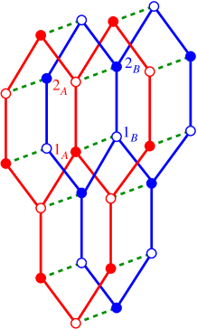
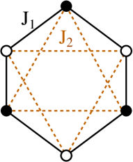
Figure 1: The $J_{1}$–$J_{2}$–$J_{1}^{\perp}$ model on the honeycomb bilayer lattice, showing (a) the two layers $A$ (red) and $B$ (blue), the nearest-neighbor bonds ($J_{1}=$ —–; $J_{1}^{\perp}=$ - - -), and the four sites ($1_{A},2_{A},1_{B},2_{B}$) of the unit cell; and (b) the intralayer bonds $J_{1}=$ —–; $J_{2}=$ - - -) on each layer. Sites on the two monolayer triangular sublattices are shown by filled and empty circles respectively.

The corresponding $AA$-stacked bilayer unit cell thus contains 4 sites, as shown explicitly in Fig. 1(a). The three types of AFM bonds are also shown in Fig. 1.

Let us first consider the classical limit ($s\rightarrow\infty$) of the model. For the honeycomb-lattice monolayer (i.e., for $\delta=0$) Néel AFM order (i.e., where all spins on lattice sites denoted by filled circles in Fig. 1 point in a given, arbitrary, direction, and those on the sites denoted by empty circles point in the opposite direction) persists for all values $\kappa\leq\frac{1}{6}$ of the intralayer frustration parameter [7, 9]. At this QCP a phase transition to a state with spiral order occurs. Indeed, the GS phase for $\kappa>\frac{1}{6}$ has a spiral wave vector that can point in an arbitrary direction. As a consequence, there now exists an infinite classical one-parameter family of states, all degenerate in energy. Spin-wave fluctuations have been shown to lift this accidental degeneracy by favouring particular wave vectors [10]. This mechanism has hence become known as spiral order by disorder.

By comparison with the classical case one would expect that in the quantum case the critical value of $\kappa$ at which Néel order melts will be larger than the classical value of $\frac{1}{6}$, since quantum fluctuations as a general rule tend to favor collinear phases over spiral phases. There is by now a wide consensus that this expectation is fulfilled by the present model, with a large number of calculations for the $s=\frac{1}{2}$ $J_{1}$–$J_{2}$ honeycomb-lattice monolayer giving a critical value of $\kappa$ for the vanishing of Néel order in the approximate range $0.17$–$0.22$ [15, 16, 18, 20, 21, 22, 23, 24, 25, 26]. There is also broad agreement, including from calculations using the CCM [20, 21] that we employ here, that spiral order is absent for the spin-$\frac{1}{2}$ case over the entire range $0\leq\kappa\leq 1$ of the frustration parameter.

If we now turn our attention to the $J_{1}$–$J_{2}$–$J_{1}^{\perp}$ model on the bilayer honeycomb lattice, at the classical level (i.e., when $s\rightarrow\infty$) the introduction of the interlayer NN coupling $J_{1}^{\perp}$ is essentially trivial. Thus, the classical (Néel and spiral) phases are totally unaffected, since the $J_{1}^{\perp}$ coupling introduces no extra frustration. The NN interlayer pairs simply anti-align (for the case when $J_{1}^{\perp}>0$, as considered here), and the order in each layer remains unchanged. However, for the quantum versions of the model (i.e., for finite values of $s$) the situation differs significantly, since for large enough values of the parameter $\delta\equiv J_{1}^{\perp}/J_{1}$, for a fixed value of the frustration parameter $\kappa\equiv J_{2}/J_{1}$, we clearly expect the GS phase to be an IDVBC phase. As we mentioned previously in Sec. 1, the CCM has been employed very recently [30] to study the GS phase diagram of the spin-$\frac{1}{2}$ $J_{1}$–$J_{2}$–$J_{1}^{\perp}$ model on a bilayer honeycomb lattice in the $\kappa\delta$ plane, particularly to find the region of stability of the Néel phase. In that earlier work it was found that the best estimate for the Néel phase boundary came from the vanishing of the calculated Néel order parameter $M$. Calculations of the triplet spin gap $\Delta$ were also performed. While these calculations corroborated the estimates from $M$, in practice they were less accurate. Our aim now is to calculate for the same system the zero-field transverse magnetic susceptibility $\chi$, in order to find further corroboration of the earlier results.

The Néel state that we envisage is clearly now one in which the spins on all of the sites in Fig. 1(a) shown by filled circles point in a given (arbitrarily chosen) direction and those on the sites shown by empty circles point in the opposite direction. Let us now apply an external magnetic field of strength $h$ in a direction perpendicular to the Néel alignment direction (and we choose units such that the gyromagnetic ratio $g\mu_{B}/\hbar=1$). The spins will thus cant at an angle $\alpha$ with respect to their zero-field configurations, and $\alpha$ may be found by minimizing the energy $E=E(h)$ in the presence of the field. The (uniform) transverse magnetic susceptibility, $\chi(h)$, is then defined, as usual, to be

$$\chi({h})=-\frac{1}{N}\frac{{\rm d}^{2}E}{{\rm d}h^{2}}\,.$$ (2)

Its zero-field limit, $\chi\equiv\chi(0)$, in which we are interested here, is one of the parameters of the effective magnon field theory that fully describes the low-energy behavior of the system. For the classical ($s\rightarrow\infty$) version of our model it is easy to calculate its value in the Néel phase to be,

$$\chi_{{\rm cl}}^{{\rm N\acute{e}el}}=\frac{1}{2J_{1}(3+\delta)}\,,$$ (3)

independent of the frustration parameter $\kappa$.

3 THE COUPLED CLUSTER METHOD

The CCM [31, 32, 33, 34, 35, 36, 37, 38, 39, 40, 41, 42, 43, 44, 45, 46] provides one of the most accurate and most adaptable ab inito techniques of modern quantum many-body theory. It is both size-consistent and size-extensive at every level of approximation, thereby ensuring that the method can be implemented in the infinite-lattice ($N\rightarrow\infty$) limit from the outset. Thus, no finite-size scaling is ever needed. Since this is often a large source of errors in many competing methods, it is a considerable advantage of using the CCM. Further advantages are that the very important Hellmann-Feynman theorem is also preserved at every level of approximation, together with the Goldstone linked-cluster theorem. These ensure that the method provides accurate, robust, and self-consistent results for a variety of calculated physical parameters for any specific system. The CCM can furthermore nowadays be implemented computationally to high orders of approximation in well-studied and well-understood truncation hierarchies that become exact as some specified parameter that describes the order of the approximation approaches infinity. The only approximation ever made in the CCM is thus to extrapolate the sequences of calculated approximants for any specified parameter of the system in which we are interested. By now there are well-studied and well-understood extrapolation schemes available for a wide variety of physical parameters.

For present purposes we will very briefly review here only some of the principal and most pertinent features of the CCM as it is applied to quantum spin-lattice models, and refer the interested reader to the by now very extensive literature (and see, e.g., Refs. [45, 46] in particular) for full details. In order to utilize the CCM in practice, the first step is always to choose a suitable model (or reference) state $|\Phi\rangle$, which acts as a generalized vacuum state, and with respect to which the quantum correlations present in the exact GS wave function $|\Psi\rangle$ can then later be incorporated in a systematic way. For spin-lattice systems all (quasi)classical states with perfect magnetic LRO provide suitable such model states. Here we will use both the Néel state and its canted equivalent in the presence of an external transverse magnetic field as our CCM model states. For later purposes it is extremely convenient to be able to consider all lattice spins as being fully equivalent to each other in every model state. In particular, this will then allow us to use a universal computational technique that is suitable for any spin-lattice model (at least initially for the phases with quasiclassical order) [57]. An obvious way to do this is clearly to make a passive rotation of each spin separately (in any such classical model state) so that, in their own set of local spin-coordinate frames, they all point in the same direction, say downwards (i.e., along the local negative $z_{s}$ axis). Every model state will thus take the universal from $|\Phi\rangle=|\downarrow\downarrow\downarrow\cdots\downarrow\rangle$ in its own set of local frames. Evidently we still need to rewrite the Hamiltonian of the system as appropriate in the specific choice of local spin-coordinate frames.

The exact GS wave function $|\Psi\rangle$, where $H|\Psi\rangle=E|\Psi\rangle$, is now expressed within the CCM in the exponentiated form,

$$|\Psi\rangle={\rm e}^{S}|\Phi\rangle\,;\quad S=\sum_{I\neq 0}{\cal S}_{I}C^{+}_{I}\,,$$ (4)

that is distinctive for the method. The set-index $I$ represents a multispin configuration, such that the set of states $\{C_{I}^{+}|\Phi\rangle\}$ completely spans the ket-state Hilbert space. We choose $C^{+}_{0}\equiv 1$ to be the identity operator. Clearly, with the CCM model state chosen as above to be in the universal form $|\Phi\rangle=|\downarrow\downarrow\downarrow\cdots\downarrow\rangle$ in an appropriate choice of locally rotated spin-coordinate frames, the operator $C^{+}_{I}$ now also takes the universal form of a product of single-spin raising operators, $s^{+}_{k}\equiv s^{x}_{k}+is^{y}_{k}$. The set index $I$ now is expressed as a set of lattice site indices,

$$I\equiv\{k_{1},k_{2},\cdots,k_{n};\;\quad n=1,2,\cdots,2sN\}\,,$$ (5)

in which no given site index $k_{i}$ may appear more than $2s$ times (for spins of general spin quantum number $s$). The operator $C^{+}_{I}$ thereby creates a multispin configuration cluster,

$$C^{+}_{I}\equiv s^{+}_{k_{1}}s^{+}_{k_{2}}\cdots s^{+}_{k_{n}};\;\quad n=1,2,\cdots,2sN\,.$$ (6)

The model state $|\Phi\rangle$ and the complete set of mutually commuting multispin creation operators $\{C_{I}^{+}\}$,

$$[C^{+}_{I},C^{+}_{J}]=0\,,\quad\forall I,J\,,$$ (7)

are hence chosen so that $|\Phi\rangle$ is a fiducial vector (or generalized vacuum state) with respect to the set $\{C_{I}^{+}\}$, and hence so that the latter obey the conditions,

$$\langle\Phi|C^{+}_{I}=0=C^{-}_{I}|\Phi\rangle\,,\quad\forall I\neq 0\,,$$ (8)

where $C^{-}_{I}\equiv(C^{+}_{I})^{\dagger}$ is the corresponding multispin destruction operators. The states $\{C_{I}^{+}|\Phi\rangle\}$ are also usefully orthonormalized, so that they obey the relations

$$\langle\Phi|C_{I}^{-}C_{J}^{+}|\Phi\rangle=\delta_{I,J}\,,\quad\forall I,J\neq 0\,,$$ (9)

with $\delta_{I,J}$ defined as a generalized Kronecker symbol.

We note that the model state $|\Phi\rangle$ is (always) chosen to be normalized, $\langle\Phi|\Phi\rangle=1$, and the CCM parametrization of Eq. (4) automatically ensures that the exact GS energy eigenket $|\Psi\rangle$ obeys the intermediate normalization condition, $\langle\Phi|\Psi\rangle=1$, due to Eq. (8). In general, of course, $\langle\Psi|\Psi\rangle\neq 1$. The corresponding GS energy eigenbra $\langle\tilde{\Psi}|$, which obeys the Schrödinger equation $\langle\tilde{\Psi}|H=E\langle\tilde{\Psi}|$, takes the CCM parametrization,

$$\langle\tilde{\Psi}|=\langle\Phi|\tilde{S}{\rm e}^{-S}\,,\quad\tilde{S}=1+\sum_{I\neq 0}\tilde{{\cal S}}_{I}C^{-}_{I}\,.$$ (10)

Equation (10) ensures the automatic fulfillment of the normalization condition $\langle\tilde{\Psi}|\Psi\rangle=1$. While Hermiticity clearly implies that the CCM correlation correlation operators $S$ and $\tilde{S}$ are connected via the relation,

$$\langle\Phi|\tilde{S}=\frac{\langle\Phi|{\rm e}^{S^{\dagger}}{\rm e}^{S}}{\langle\Phi|{\rm e}^{S^{\dagger}}{\rm e}^{S}|\Phi\rangle}\,,$$ (11)

a key feature of the CCM is that this constraint is not explicitly imposed. Instead the $c$-number parameters $\{{\tilde{\cal S}}_{I}\}$ are considered to be formally independent of their $\{{\cal S}_{I}\}$ counterparts. Clearly, the Hermiticity constraint of Eq. (11) will be exactly fulfilled in the exact limit when all multispin clusters specified by the complete set of indices $\{I\}$ are retained in the CCM expansions of Eqs. (4) and (10). However, in practice, when approximations are made, as described below, to restrict ourselves to some suitable subset of the indices $\{I\}$, Hermiticity may only approximately be fulfilled. Nevertheless, it is very important to realize that this partial loss of exact Hermiticity is always more than compensated in practice by the exact fulfillment of the Hellmann-Feynman theorem at every level of approximation.

All GS physical quantities may now be expressed entirely in terms of the CCM correlation coefficients $\{{\cal S}_{I},\tilde{{\cal S}}_{I}\}$. For example, the GS magnetic order parameter $M$, which is just the average local on-site magnetization, may be expressed as

$$M=-\frac{1}{N}\langle\Phi|\tilde{S}\sum^{N}_{k=1}{\rm e}^{-S}s^{z}_{k}{\rm e}^{S}|\Phi\rangle\,.$$ (12)

where $s_{k}^{z}$ is expressed in the local (rotated) spin-coordinate frames described above. The parameters $\{{\cal S}_{I},\tilde{{\cal S}}_{I}\}$ are themselves now formally obtained by minimization of the energy expectation functional,

$$\bar{H}=\bar{H}[{\cal S}_{I},{\tilde{\cal S}_{I}}]\equiv\langle\Phi|\tilde{S}{\rm e}^{-S}H{\rm e}^{S}|\Phi\rangle\,,$$ (13)

with respect to each of them, considered as independent variables.

Thus, firstly, using the explicit parametrization of Eq. (10), extremization of $\bar{H}$ from Eq. (13) with respect to the parameter ${\tilde{\cal S}}_{I}$, yields the relations

$$\langle\Phi|C^{-}_{I}{\rm e}^{-S}H{\rm e}^{S}|\Phi\rangle=0\,,\quad\forall I\neq 0\,.$$ (14)

Equation (14) is simply a coupled set of nonlinear equations for the creation coefficients $\{{\cal S}_{I}\}$, with as many equations as there are unknown. Secondly, using the explicit CCM parametrization of Eq. (4), extremization of $\bar{H}$ from Eq. (13) with respect to the parameters ${\cal S}_{I}$, yields the respective relations

$$\langle\Phi|\tilde{S}{\rm e}^{-S}[H,C^{+}_{I}]{\rm e}^{S}|\Phi\rangle=0\,,\quad\forall I\neq 0\,.$$ (15)

By making use of the simple relation $[S,C_{I}^{+}]=0$, which follows trivially from Eqs. (4) and (7), Eq. (15) may readily be expressed in the equivalent form,

$$\langle\Phi|\tilde{S}({\rm e}^{-S}H{\rm e}^{S}-E)C^{+}_{I}|\Phi\rangle=0\,,\quad\forall I\neq 0\,,$$ (16)

where we have re-expressed the GS ket-state Schrödinger equation in the form,

$${\rm e}^{-S}H{\rm e}^{S}|\Phi\rangle=E|\Phi\rangle\,,$$ (17)

using Eq. (4). Equation (16) is thus a set of generalized linear eigenvalue equations for the destruction coefficients $\{{\tilde{\cal S}_{I}}\}$, with the coefficients $\{{\cal S}_{I}\}$ as known input from first solving Eq. (14), again with as many equations as unknowns.

We note that the exponentiated forms ${\rm e}^{\pm S}$, which are such a characteristic and distinctive element of the CCM, always only enter in the form of a similarity transform ${\rm e}^{-S}\Omega{\rm e}^{S}$ of some operator $\Omega$, where $\Omega=H$ in Eqs. (14) and (16), which are the equations to be solved for $\{{\cal S}_{I},{\tilde{\cal S}}_{I}\}$, and $\Omega=s_{k}^{z}$ in Eq. (12) for the evaluation of the order parameter $M$, for example. Such similarity-transformed operators may be expanded as the well-known nested commutator sums

$${\rm e}^{-S}\Omega{\rm e}^{S}=\sum_{n=0}^{\infty}\frac{1}{n!}[\Omega,S]_{n}\,,$$ (18)

where $[\Omega,S]_{n}$ is the $n$-fold nested commutator, defined iteratively as

$$[\Omega,S]_{n}=[[\Omega,S]_{n-1},S]\,;\quad[\Omega,S]_{0}=S\,.$$ (19)

It is important to realize that in practice, for all usual choices of the operator $\Omega$, the otherwise infinite sum in Eq. (18) will actually terminate exactly at a (low) finite order. The reasons for this are that the operator $\Omega$ usually contains only finite-order multinomial terms in the corresponding sets of single-spin operators (as for $H$ here), and that all of the elements in the decomposition of $S$ in Eq. (4) mutually commute. The SU(2) commutation relations for the spin operators then readily imply that the sum in Eq. (18) will terminate after a finite number of terms.

Thus, the only approximation that we need to make in order to implement the CCM is to restrict the set of multispin-flip configurations $\{I\}$ that we retain in the expansions of Eqs. (4) and (10) for the correlation operators $S$ and $\tilde{S}$, respectively, to some manageable subset. A well-tested such hierarchical scheme, which we will adopt here, is the so-called localized lattice-animal-based subsystem (LSUB$n$) scheme. It retains all such multispin configurations that, at the $n$th level of approximation, describe clusters of spins spanning a range of no more than $n$ contiguous sites. In this sense a set of lattice sites is said to be contiguous if every site in the set is NN to at least one other in the set (in some specified geometry that defines NN pairs). Hence, the configurations retained in the LSUB$n$ scheme are those defined on all possible (polyominos or) lattice animals up to size $n$. Obviously, as the truncation index grows without bound (i.e., as $n\rightarrow\infty$) the corresponding LSUB$\infty$ limit is the exact result.

The space- and point-group symmetries of the lattice and of the model state $|\Phi\rangle$ under study, together with any relevant conservation laws, are used to minimize the effective size of the index set $\{I\}$ that is retained at each LSUB$n$ level. For example, for our present Heisenberg interactions contained in Eq. (1) and for the Néel model state (in zero-external field), the total $z$-component of spin, $s_{T}^{z}\equiv\sum_{k=1}^{N}s_{k}^{z}$, is a conserved quantity, where global spin axes are assumed, and hence we retain only multispin configurations for the GS Néel phase with $s_{T}^{z}=0$. Even after incorporating all such symmetries and conservation laws, the number $N_{f}=N_{f}(n)$ of distinct, nonzero fundamental configurations that are included at a given $n$th level of LSUB$n$ approximation grows rapidly (and typically, super-exponentially) as a function of the truncation index $n$. For the Néel GS of the spin-$\frac{1}{2}$ honeycomb-lattice monolayer, for example, we have $N_{f}(10)=6\,237$ and $N_{f}(12)=103\,097$. For the corresponding bilayer case we have $N_{f}(8)=2\,560$ and $N_{f}(10)=70\,118$. By contrast, the canted Néel state (i.e., in the presence of a transverse magnetic field) has less symmetries and hence the number $N_{f}(n)$ for the calculation of the susceptibility $\chi$ is appreciably higher than the corresponding number for the calculation of the magnetic order parameter $M$ at the same level $n$ of approximation. Thus, for the spin-$\frac{1}{2}$ honeycomb lattice monolayer, for the case of the canted Néel state as our CCM model state, we have $N_{f}(8)=3\,304$ and $N_{f}(10)=58\,337$, whereas the for corresponding bilayer case we have $N_{f}(6)=1\,494$ and $N_{f}(8)=43\,338$.

Clearly, the use of both massive parallelization and supercomputing resources is required for the derivation and solution of such large sets of CCM equations for the GS correlation coefficients $\{{\cal S}_{I},\tilde{{\cal S}}_{I}\}$. We also use a purpose-built and customized computer-algebra package [57] for the derivation of the equations to be solved [i.e., Eqs. (14) and (16)]. Previous work [30] on the current model, based on the Néel state as CCM model state, was able to perform LSUB$n$ calculations for the order parameter $M$, for example, for values $n\leq 10$. Due to the substantially decreased symmetry of the canted Néel state, by contrast we are now able to perform calculations for the transverse magnetic susceptibility $\chi$ only for values $n\leq 8$.

The last step, and sole approximation, is now to extrapolate our LSUB$n$ sequences of approximants for the calculated physical parameters to the (exact) $n\rightarrow\infty$ limit. For example, for systems that display a GS order-disorder QPT, a well-tested and accurate extrapolation scheme for the magnetic order parameter $M$ of Eq. (12) has been found to be given by (and see, Refs. [5, 19, 20, 21, 30, 47, 48, 49])

$$M(n)=\mu_{0}+\mu_{1}n^{-1/2}+\mu_{2}n^{-3/2}\,.$$ (20)

This scheme, which is also appropriate for phases whose magnetic order parameter $M$ is zero or small, yields the respective LSUB$\infty$ extrapolant $\mu_{0}$ for $M$. By contrast, a scheme with a leading exponent of -1 [rather than the value $-\frac{1}{2}$ for $M$ in Eq. (20)] has been found (and see, e.g., Refs. [53, 54, 58, 59, 60]) to give excellent results for the zero-field transverse (uniform) magnetic susceptibility of Eq. (2) with $h=0$,

$$\chi(n)=x_{0}+x_{1}n^{-1}+x_{2}n^{-2}\,.$$ (21)

This scheme thus leads to the LSUB$\infty$ extrapolant $x_{0}$ as our value for $\chi$.

Clearly, for each of the extrapolation schemes such as those in Eqs. (20) and (21), each of which involves three fitting parameters, it is preferable to use four or more input data points (i.e., LSUB$n$ approximants with different values of the truncation parameter $n$). However, the LSUB2 result is usually likely to be too far removed from the $n\rightarrow\infty$ limit to be useful in the fits, if it can be avoided. Nevertheless, as we have remarked above, it is computationally infeasible to perform LSUB$n$ calculations of $\chi$ for the spin-$\frac{1}{2}$ honeycomb bilayer for values $n>8$. For these reasons our preferred set of fitting values are those with $n=\{4,6,8\}$. However, in all cases we have also performed separate fits using data sets with $n=\{2,4,6,8\}$. The differences in the extrapolated values are generally extremely small.

4 RESULTS

We first show, in Fig. 2, our results for the zero-field transverse magnetic susceptibility $\chi$ as a function of the intralayer frustration parameter $\kappa$, for three respective values of the interlayer coupling parameter $\delta$.

 

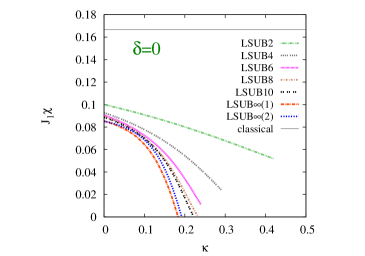
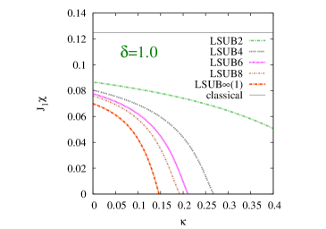
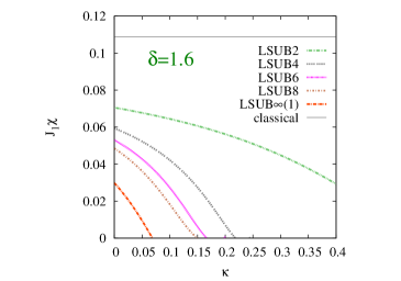
Figure 2: CCM results for the zero-field transverse magnetic susceptibility $\chi$ (in units of $J_{1}^{-1}$) versus the frustration parameter $\kappa\equiv J_{2}/J_{1}$, for the spin-$\frac{1}{2}$ $J_{1}$–$J_{2}$–$J_{1}^{\perp}$ model on the bilayer honeycomb lattice (with $J_{1}>0$), for three selected values of the scaled interlayer exchange coupling constant, $\delta\equiv J_{1}^{\perp}/J_{1}$: (a) $\delta=0$, (b) $\delta=1.0$, and (c) $\delta=1.6$. Results based on the (canted) Néel state as CCM model state are shown in LSUB$n$ approximations with $n=2,4,6,8$ (and also with $n=10$ for the special case of the $J_{1}$–$J_{2}$ monolayer, i.e., when $\delta=0$), together with various corresponding LSUB$\infty(i)$ extrapolated results using Eq. (21) and the respective data sets $n=\{4,6,8\}$ for $i=1$ and $n=\{4,6,8,10\}$ for $i=2$ (for the case $\delta=0$ only).

In each case we also show the corresponding classical result from Eq. (3), which is now independent of $\kappa$ and thus takes a constant value in each case. For each of the three values of $\delta$ shown in Figs. 2(a), 2(b), and 2(c) we display our LSUB$n$ results for values $n=2,4,6,8$, together with the LSUB$\infty(1)$ extrapolant $x_{0}$ obtained from fitting Eq. (21) to the data set $n=\{4,6,8\}$. Uniquely, for the case $\delta=0$ shown in Fig. 2(a), which corresponds to the honeycomb-lattice monolayer, we are also able to perform calculations at the LSUB10 level, which we also display there, together with a separate LSUB$\infty(2)$ extrapolant $x_{0}$ obtained from fitting Eq. (21) to the data set $n=\{4,6,8,10\}$. Clearly, the two extrapolations LSUB$\infty(1)$ and LSUB$\infty(2)$ are in excellent agreement with each other.

Each of the cases shown in Fig. 2, for the three separate values of $\delta$, illustrates that the quantum $(s=\frac{1}{2})$ values for $\chi$ are always substantially below the corresponding classical $(s\rightarrow\infty)$ values. More striking, however, is that in each case there is a critical value $\kappa_{c}(\delta)$ at which the extrapolated value for $\chi$ vanishes. It is also clear from the case $\delta=0$ shown in Fig. 2(a) that our extrapolations are quite robust with respect to which LSUB$n$ data input sets are used. The vanishing of $\chi$, due to the strong effects of quantum correlations, is, as we have noted in Sec. 1, a very clear indication of the opening of a spin gap at this point [55, 56], and we may hence take it as an indicator of the QCP at which Néel order melts.

The three cases shown in Fig. 2 reveal that this critical value $\kappa_{c}(\delta)$ at which Néel order vanishes decreases as the strength $\delta$ of the interlayer coupling increases, at least for values of $\delta$ above a certain lower critical value, to which we return in more detail below. In Fig. 3 we show the effect of the interlayer coupling separately, now for three illustrative values of the intralayer frustration parameter $\kappa$.

 

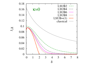
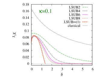
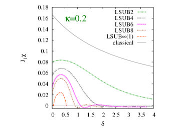
Figure 3: CCM results for the zero-field transverse magnetic susceptibility $\chi$ (in units of $J_{1}^{-1}$) versus the scaled interlayer exchange coupling constant, $\delta\equiv J_{1}^{\perp}/J_{1}$, for the spin-$\frac{1}{2}$ $J_{1}$–$J_{2}$–$J_{1}^{\perp}$ model on the bilayer honeycomb lattice (with $J_{1}>0$), for three selected values of the intralayer frustration parameter, $\kappa\equiv J_{2}/J_{1}$: (a) $\kappa=0$, (b) $\kappa=0.1$, and (c) $\kappa=0.2$. Results based on the (canted) Néel state as CCM model state are shown in LSUB$n$ approximations with $n=2,4,6,8$, together with corresponding LSUB$\infty(1)$ extrapolated results using Eq. (21), with the data sets $n=\{4,6,8\}$.

In each case we show our CCM LSUB$n$ results with values $n=2,4,6,8$ of the truncation parameter, as well as the extrapolated value $x_{0}$ obtained from fitting the data points $n=\{4,6,8\}$ to Eq. (21), We also show the corresponding classical curves obtained from Eq. (3). Once again we see that the effects of quantum correlations in the $s=\frac{1}{2}$ case are to reduce the value of $\chi$ substantially from its classical ($s\rightarrow\infty$) value.

Figure 3(a) shows our results for the case $\kappa=0$ (i.e., without intralayer frustration), where NN AFM interactions alone are present. We observe the interesting feature that as $\delta$ is slowly increased from zero the effect is first to increase the value of $\chi$ both in absolute value and to bring it closer to the corresponding classical value at the same value of $\delta$. This is presumably because the effects of quantum correlations first weaken as $\delta$ is increased from zero, thereby increasing the stability of Néel magnetic LRO. This enhancement reaches a maximum for each LSUB$n$ level of approximation (except for the lowest-order, $n=2$) at a value $\delta\approx 0.5$. Néel LRO then reduces as $\delta$ is increased further. At every LSUB$n$ level $\chi$ then tends asymptotically to zero. It is evident that as $n$ increases this asymptotic vanishing of $\chi$ becomes sharper and sharper, ultimately as fully reflected in the LSUB$\infty(1)$ extrapolant that vanishes at the value $\delta_{c}^{>}(\kappa=0)\approx 2.076$. This agrees reasonably well with a corresponding estimate $\delta_{c}^{>}(\kappa=0)\approx 1.645$ from a QMC calculation [27], which can be performed only in the case of zero frustration ($\kappa=0$), when the “minus-sign problem” is absent.

We may also compare our result for $\chi$ itself for the limiting case $\kappa=0=\delta$ of a pure honeycomb-monolayer HAF with only NN interactions. Our extrapolated LSUB$\infty(1)$ result based on the extrapolation scheme of Eq. (21) fitted to LSUB$n$ data points with $n=\{4,6,8\}$ gives the value $\chi(\kappa=0,\delta=0)\approx 0.0852/J_{1}$. For this limiting case alone we have also performed LSUB$n$ calculations with $n=10,12$ [53]. For the LSUB12 calculation of $\chi$ using the canted Néel state as CCM model state, for example, the number of fundamental configurations is $N_{f}(12)=1\,090\,448$. The corresponding extrapolant using the LSUB$n$ input data set with $n=\{6,8,10,12\}$ is $\chi(\kappa=0,\delta=0)\approx 0.0847/J_{1}$, which again illustrates the robustness of our results. We are again in good agreement with a corresponding result $\chi(\kappa=0,\delta=0)\approx 0.0778/J_{1}$ that was extracted (and see Ref. [53] for details on how to do so) from a published QMC calculation of Löw [61] for this unfrustrated case.

In Figs. 3(b) and 3(c) comparable results to those in Fig. 3(a) for the unfrustrated case ($\kappa=0$) are also shown for the two cases when $\kappa=0.1$ and $\kappa=0.2$, respectively. As we would expect, as $\kappa$ is increased quantum correlations become stronger and the susceptibility $\chi$ is reduced. Correspondingly, the upper critical value $\delta_{c}^{>}(\kappa)$ above which a gapped state appears decreases monotonically with increasing values of $\kappa$. From the LSUB$\infty(1)$ extrapolation in Fig. 2(a) we see that $\kappa_{c}(0)\approx 0.183$, which is below the value $\kappa=0.2$ shown in Fig. 3(c). What we now observe, very interestingly, is that for values $\kappa>\kappa_{c}(0)$ that are not too large, Néel order is re-established as $\delta$ is increased above a lower critical $\delta_{c}^{<}(\kappa)$, while remaining below the upper critical value $\delta_{c}^{>}(\kappa)$, leading to the sort of reentrant behavior seen in Fig. 3(c). For the case $\kappa=0.2$ shown there, for example, the LSUB$\infty(1)$ extrapolation gives the values $\delta_{c}^{<}(0.2)\approx 0.046$ and $\delta_{c}^{>}(0.2)\approx 0.567$. Finally, as $\kappa$ is further increased we arrive at an upper critical value $\kappa^{>}$ such that $\delta_{c}^{<}(\kappa^{>})=\delta_{c}^{>}(\kappa^{>})$, and for all values $\kappa>\kappa^{>}$ a gapped paramagnetic state is present, whatever the value of $\delta$, at least immediately beyond the boundary of Néel stability. Our LSUB$\infty(1)$ extrapolations for $\chi$ lead to a value $\kappa^{>}\approx 0.212$, with $\delta_{c}^{<}(\kappa^{>})=\delta_{c}^{>}(\kappa^{>})\approx 0.25(5)$.

Finally, in Fig. 4, we use our extrapolated LSUB$\infty(1)$ results for $\chi$ such as those shown in Figs. 2 and 3 to delineate the Néel phase boundary as the points where $\chi\rightarrow 0$.

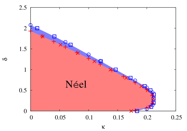
Figure 4: $T=0$ phase diagram of the spin-$\frac{1}{2}$ $J_{1}$–$J_{2}$–$J_{1}^{\perp}$ model on the bilayer honeycomb lattice with $J_{1}>0$, $\delta\equiv J_{1}^{\perp}/J_{1}$, and $\kappa\equiv J_{2}/J_{1}$. The blue open square ($\square$) symbols and the blue open circle plus ($\circ$) symbols are points at which the extrapolated zero-field transverse magnetic susceptibility for the Néel phase vanishes, for specified values of $\delta$ and $\kappa$, respectively. They thus represent the values $\kappa_{c}(\delta)$ and $\delta_{c}^{>}(\kappa)$ [and also $\delta_{c}^{<}(\kappa)$ for values of $\kappa$ in the range $\kappa_{c}(0)<\kappa<\kappa^{>}$], respectively. In each case the (canted) Néel state is used as CCM model state, and Eq. (21) is used for the extrapolations with the corresponding LSUB$n$ data sets $n=\{4,6,8\}$. For comparison we also show by the red cross ($\times$) symbols and the red plus ($+$) symbols the points at which the extrapolated GS magnetic order parameter $M$ for the Néel phase vanishes, for specified values of $\delta$ and $\kappa$, respectively. In each case the Néel state is used as CCM model state, and Eq. (20) is used for the extrapolations with the same LSUB$n$ data sets $n=\{4,6,8\}$.

Different symbols are used to indicate the results for $\kappa_{c}(\delta)$ at fixed values of $\delta$, as obtained from curves such as those shown in Fig. 2, and for both $\delta_{c}^{>}(\kappa)$ and $\delta_{c}^{<}(\kappa)$ (the latter in the case only when $\kappa_{c}(0)<\kappa<\kappa^{>}$), as obtained from curves such as those shown in Fig. 3 for fixed values of $\kappa$. The overall accuracy of our results can be estimated from the fact that points on the Néel phase boundary from two independent sets of results agree so well with one another. On Fig. 4, for comparison purposes, we also plot similar sets of points at which the corresponding LSUB$\infty(1)$ extrapolants for the magnetic order parameter $M$ [i.e., as determined from Eq. (20) and LSUB$n$ data sets with $n=\{4,6,8\}$ used as input] vanish (and see Ref. [30]). It is extremely gratifying that the Néel phase boundaries obtained from the points where $\chi$ and $M$ vanish, respectively, are in such overall excellent agreement.

5 DISCUSSION AND SUMMARY

We have used the CCM and its well-defined and systematic LSUB$n$ hierarchy of approximations to investigate the Néel phase boundary in the $T=0$ quantum phase diagram in the $\kappa\delta$ plane of the spin-$\frac{1}{2}$ $J_{1}$–$J_{2}$–$J_{1}^{\perp}$ model on a bilayer honeycomb lattice. In particular, we have used the canted Néel state (obtained from placing the Néel-ordered system in a transverse external magnetic field) as our CCM model state in order to calculate $\chi$, the transverse (uniform) magnetic susceptibility in the zero-field limit. Unlike in the classical ($s\rightarrow\infty$) version of the model, where $\chi$ never vanishes, we find that for the $s=\frac{1}{2}$ model quantum correlations become sufficiently strong to make $\chi\rightarrow 0$ along a curve in the $\kappa\delta$ plane. All such points where $\chi$ vanishes mark the emergence of a new gapped phase, and hence the melting of Néel LRO. We have exactly calculated $\chi=\chi(\kappa,\delta)$ at high-order LSUB$n$ truncations with $n\leq 8$, and as our sole approximation have extrapolated the sequences of LSUB$n$ values for $\chi$ at given values of $\kappa$ and $\delta$ with $n=\{4,6,8\}$, via a well-understood and well-tested extrapolation scheme, to the limit $n\rightarrow\infty$ where the method becomes exact in principle. At all points along the Néel phase boundary we have thereby seen that quasiclassical magnetic LRO gives way to a nonclassical paramagnetic gapped state, which is almost certainly a VBC state of one sort or another, and which almost certainly differ as one moves along the boundary. Thus, for the large-$\delta$ region (for fixed values of $\kappa$) the Néel state will certainly melt into a GS with IDVBC order, while for very small values of $\delta$ it is most likely that the emergent gapped state will have plaquette VBC (PVBC) order, as is generally agreed to be the correct phase for the monolayer ($\delta=0$) for values of $\kappa$ beyond $\kappa_{c}(0)$ (and see, e.g., Refs. [20, 21]).

Perhaps the most striking feature of the phase diagram of Fig. 4 is the marked reentrant behavior, whereby for values of the intralayer frustration parameter in the range $\kappa_{c}(0)<\kappa<\kappa^{>}$ there exists a range of values of the interlayer coupling, $\delta_{c}^{<}(\kappa)<\delta<\delta_{c}^{>}(\kappa)$ in which Néel LRO is present. Inside this region, which has larger values of frustration present than the maximum allowed value $\kappa_{c}(0)$ for Néel order in the monolayer, the effect of the bilayer coupling is to enhance the Néel order to the extent that it reappears. Beyond a maximum value, $\kappa>\kappa^{>}$, however, no amount of interlayer coupling suffices to re-establish Néel LRO.

We have also compared the Néel phase boundary that we have obtained from the vanishing of $\chi$ with that obtained directly from the vanishing of the Néel order parameter $M$. In order to make a valid comparison we have compared two completely independent sets of CCM calculations for each quantity, both extrapolated with the same sets of LSUB$n$ data with $n=\{4,6,8\}$ as input. Figure 4 shows the excellent level of agreement, which, in turn, reinforces that at all points on the Néel phase boundary shown, quasiclassical magnetic order gives way to a nonclassical paramagnetic state with a nonzero energy gap to the lowest excited state. This is one of the most important findings of the present study.

References

- Sachdev [2008] S. Sachdev, Nat. Phys. 4, 173–185 (2008).
- Sachdev [2011] S. Sachdev, Quantum Phase Transitions, 2nd ed. (Cambridge University Press, Cambridge, UK, 2011).
- Mermin and Wagner [1966] N. D. Mermin and H. Wagner, Phys. Rev. Lett. 17, 1133–1136 (1966).
- Richter, Schulenburg, and Honecker [2004] J. Richter, J. Schulenburg, and A. Honecker, in Quantum Magnetism, Lecture Notes in Physics Vol. 645, edited by U. Schollwöck, J. Richter, D. J. J. Farnell, and R. F. Bishop (Springer-Verlag, Berlin, 2004) , pp. 85–153.
- Farnell et al. [2014] D. J. J. Farnell, O. Götze, J. Richter, R. F. Bishop, and P. H. Y. Li, Phys. Rev. B 89, p. 184407 (2014).
- Troyer, Kontani, and Ueda [1996] M. Troyer, H. Kontani, and K. Ueda, Phys. Rev. Lett. 76, 3822–3825 (1996).
- Rastelli, Tassi, and Reatto [1979] E. Rastelli, A. Tassi, and L. Reatto, Physica B & C 97, 1–24 (1979).
- Mattsson, Fröjdh, and Einarsson [1994] A. Mattsson, P. Fröjdh, and T. Einarsson, Phys. Rev. B 49, 3997–4002 (1994).
- Fouet, Sindzingre, and Lhuillier [2001] J. B. Fouet, P. Sindzingre, and C. Lhuillier, Eur. Phys. J. B 20, 241–254 (2001).
- Mulder et al. [2010] A. Mulder, R. Ganesh, L. Capriotti, and A. Paramekanti, Phys. Rev. B 81, p. 214419 (2010).
- Ganesh et al. [2011a] R. Ganesh, D. N. Sheng, Y.-J. Kim, and A. Paramekanti, Phys. Rev. B 83, p. 144414 (2011a).
- Ganesh et al. [2011b] R. Ganesh, D. N. Sheng, Y.-J. Kim, and A. Paramekanti, Phys. Rev. B 83, p. 219903(E) (2011b).
- Clark, Abanin, and Sondhi [2011] B. K. Clark, D. A. Abanin, and S. L. Sondhi, Phys. Rev. Lett. 107, p. 087204 (2011).
- Reuther, Abanin, and Thomale [2011] J. Reuther, D. A. Abanin, and R. Thomale, Phys. Rev. B 84, p. 014417 (2011).
- Albuquerque et al. [2011] A. F. Albuquerque, D. Schwandt, B. Hetényi, S. Capponi, M. Mambrini, and A. M. Läuchli, Phys. Rev. B 84, p. 024406 (2011).
- Mosadeq, Shahbazi, and Jafari [2011] H. Mosadeq, F. Shahbazi, and S. A. Jafari, J. Phys.: Condens. Matter 23, p. 226006 (2011).
- Oitmaa and Singh [2011] J. Oitmaa and R. R. P. Singh, Phys. Rev. B 84, p. 094424 (2011).
- Mezzacapo and Boninsegni [2012] F. Mezzacapo and M. Boninsegni, Phys. Rev. B 85, p. 060402(R) (2012).
- Li et al. [2012a] P. H. Y. Li, R. F. Bishop, D. J. J. Farnell, and C. E. Campbell, Phys. Rev. B 86, p. 144404 (2012a).
- Bishop et al. [2012] R. F. Bishop, P. H. Y. Li, D. J. J. Farnell, and C. E. Campbell, J. Phys.: Condens. Matter 24, p. 236002 (2012).
- Bishop, Li, and Campbell [2013] R. F. Bishop, P. H. Y. Li, and C. E. Campbell, J. Phys.: Condens. Matter 25, p. 306002 (2013).
- Zhang and Lamas [2013] H. Zhang and C. A. Lamas, Phys. Rev. B 87, p. 024415 (2013).
- Ganesh, van den Brink, and Nishimoto [2013] R. Ganesh, J. van den Brink, and S. Nishimoto, Phys. Rev. Lett. 110, p. 127203 (2013).
- Zhu, Huse, and White [2013] Z. Zhu, D. A. Huse, and S. R. White, Phys. Rev. Lett. 110, p. 127205 (2013).
- Gong et al. [2013] S.-S. Gong, D. N. Sheng, O. I. Motrunich, and M. P. A. Fisher, Phys. Rev. B 88, p. 165138 (2013).
- Yu et al. [2014] X.-L. Yu, D.-Y. Liu, P. Li, and L.-J. Zou, Physica E 59, 41–49 (2014).
- Ganesh, Isakov, and Paramekanti [2011] R. Ganesh, S. V. Isakov, and A. Paramekanti, Phys. Rev. B 84, p. 214412 (2011).
- Zhang, Arlego, and Lamas [2014] H. Zhang, M. Arlego, and C. A. Lamas, Phys. Rev. B 89, p. 024403 (2014).
- Arlego, Lamas, and Zhang [2014] M. Arlego, C. A. Lamas, and H. Zhang, J. Phys.: Conf. Ser. 568, p. 042019 (2014).
- Bishop and Li [2017] R. F. Bishop and P. H. Y. Li, Phys. Rev. B 95, p. 134414 (2017).
- Coester [1958] F. Coester, Nucl. Phys. 7, 421–424 (1958).
- Coester and Kümmel [1960] F. Coester and H. Kümmel, Nucl. Phys. 17, 477–485 (1960).
- Čižek [1966] J. Čižek, J. Chem. Phys. 45, 4256–4266 (1966).
- Kümmel, Lührmann, and Zabolitzky [1978] H. Kümmel, K. H. Lührmann, and J. G. Zabolitzky, Phys Rep. 36C, 1–63 (1978).
- Bishop and Lührmann [1978] R. F. Bishop and K. H. Lührmann, Phys. Rev. B 17, 3757–3780 (1978).
- Bishop and Lührmann [1982] R. F. Bishop and K. H. Lührmann, Phys. Rev. B 26, 5523–5557 (1982).
- Arponen [1983] J. Arponen, Ann. Phys. (N.Y.) 151, 311–382 (1983).
- Bishop and Kümmel [1987] R. F. Bishop and H. G. Kümmel, Phys. Today 40(3), 52–60 (1987).
- Arponen, Bishop, and Pajanne [1987a] J. S. Arponen, R. F. Bishop, and E. Pajanne, Phys. Rev. A 36, 2519–2538 (1987a).
- Arponen, Bishop, and Pajanne [1987b] J. S. Arponen, R. F. Bishop, and E. Pajanne, Phys. Rev. A 36, 2539–2549 (1987b).
- Bartlett [1989] R. J. Bartlett, J. Phys. Chem. 93, 1697–1708 (1989).
- Arponen and Bishop [1991] J. S. Arponen and R. F. Bishop, Ann. Phys. (N.Y.) 207, 171–217 (1991).
- Bishop [1991] R. F. Bishop, Theor. Chim. Acta 80, 95–148 (1991).
- Bishop [1998] R. F. Bishop, in Microscopic Quantum Many-Body Theories and Their Applications, Lecture Notes in Physics Vol. 510, edited by J. Navarro and A. Polls (Springer-Verlag, Berlin, 1998) , pp. 1–70.
- Zeng, Farnell, and Bishop [1998] C. Zeng, D. J. J. Farnell, and R. F. Bishop, J. Stat. Phys. 90, 327–361 (1998).
- Farnell and Bishop [2004] D. J. J. Farnell and R. F. Bishop, in Quantum Magnetism, Lecture Notes in Physics Vol. 645, edited by U. Schollwöck, J. Richter, D. J. J. Farnell, and R. F. Bishop (Springer-Verlag, Berlin, 2004) , pp. 307–348.
- Farnell et al. [2011] D. J. J. Farnell, R. F. Bishop, P. H. Y. Li, J. Richter, and C. E. Campbell, Phys. Rev. B 84, p. 012403 (2011).
- Li et al. [2012b] P. H. Y. Li, R. F. Bishop, D. J. J. Farnell, J. Richter, and C. E. Campbell, Phys. Rev. B 85, p. 085115 (2012b).
- Bishop and Li [2012] R. F. Bishop and P. H. Y. Li, Phys. Rev. B 85, p. 155135 (2012).
- Bishop, Li, and Campbell [2014a] R. F. Bishop, P. H. Y. Li, and C. E. Campbell, Phys. Rev. B 89, p. 214413 (2014a).
- Li, Bishop, and Campbell [2014] P. H. Y. Li, R. F. Bishop, and C. E. Campbell, Phys. Rev. B 89, p. 220408(R) (2014).
- Bishop, Li, and Campbell [2014b] R. F. Bishop, P. H. Y. Li, and C. E. Campbell, AIP Conf. Proc. 1619, 40–50 (2014b).
- Bishop et al. [2015] R. F. Bishop, P. H. Y. Li, O. Götze, J. Richter, and C. E. Campbell, Phys. Rev. B 92, p. 224434 (2015).
- Bishop and Li [2016] R. F. Bishop and P. H. Y. Li, J. Magn. Magn. Mater. 407, 348–357 (2016).
- Mila [2000] F. Mila, Eur. J. Phys. 21, 499–510 (2000).
- Bernu and Lhuillier [2015] B. Bernu and C. Lhuillier, Phys. Rev. Lett. 114, p. 057201 (2015).
- [57] We use the program package CCCM of D. J. J. Farnell and J. Schulenburg, see http://www-e.uni-magdeburg.de/jschulen/ccm/index.html.
- Darradi et al. [2008] R. Darradi, O. Derzhko, R. Zinke, J. Schulenburg, S. E. Krüger, and J. Richter, Phys. Rev. B 78, p. 214415 (2008).
- Farnell et al. [2009] D. J. J. Farnell, R. Zinke, J. Schulenburg, and J. Richter, J. Phys.: Condens. Matter 21, p. 406002 (2009).
- Götze et al. [2016] O. Götze, J. Richter, R. Zinke, and D. J. J. Farnell, J. Magn. Magn. Mater. 397, 333–341 (2016).
- Löw [2009] U. Löw, Condensed Matter Physics 12, 497–506 (2009).