Dynamics of social contagions with local trend imitation

Abstract

Research on social contagion dynamics has not yet including a theoretical analysis of the ubiquitous local trend imitation (LTI) characteristic. We propose a social contagion model with a tent-like adoption probability distribution to investigate the effect of this LTI characteristic on behavior spreading. We also propose a generalized edge-based compartmental theory to describe the proposed model. Through extensive numerical simulations and theoretical analyses, we find a crossover in the phase transition: when the LTI capacity is strong, the growth of the final behavior adoption size exhibits a second-order phase transition. When the LTI capacity is weak, we see a first-order phase transition. For a given behavioral information transmission probability, there is an optimal LTI capacity that maximizes the final behavior adoption size. Finally we find that the above phenomena are not qualitatively affected by the heterogeneous degree distribution. Our suggested theory agrees with the simulation results.

1 Introduction

The study of social contagion has attracted wide attention among researchers in the field of network science [1, 2]. Studies of social contagion have focused on such subjects as behavior spreading [3], information spreading [4], and the contagion of sentiment [5], and they have been both theoretical and experimental in their exploration of the essential nature of social contagion [5, 6]. Unlike biological contagions (e.g., epidemic spreading) [7, 8, 9], social contagions have a reinforcement effect [12]. A useful approach to studying social contagions that includes the reinforcement effect is a threshold model [13, 14, 15, 16] that assumes a susceptible individual accepts a new behavior when a fraction [13] or number [17] of its neighbors greater than an adoption threshold already exhibit the behavior. This threshold model is a trivial Markovian process. Numerical simulations and theoretical analyses verify that the social reinforcement effect can alter the phase transitions of social contagions [13]. In particular, the final adoption size first grows continually and then decreases discontinually versus the average degree. Many non-Markovian social contagion models have also been developed to depict the social reinforcement effect [18, 19, 20, 21, 22, 23]. Recent research has found that social reinforcement originates in the memory of non-redundant information transmission [20, 21, 22], that the growth of the final behavior adoption size is dependent on the behavioral information transmission probability, and it changes from continuous to discontinuous when the dynamical or structural parameters are altered.

In real-world cases, the probability that an individual will adopt a new behavior may be either positively or negatively correlated with the number of neighbors who have already adopted the behavior. For example, some style-conscious people who imitate the behavior of celebrities and adopt the latest fashions may also strive to avoid anything that has become overly-popular and ubiquitous (Leibenstein calls this the “snob effect” [24]). Another example is when an individual habitually patronizes a restaurant with good food and a convivial atmosphere, but then avoids it when it becomes overly-popular and crowded. Both of these examples exhibit the local trend imitation (LTI) phenomenon [25, 26, 27], i.e., the adoption probability first increases with an increase in the number or fraction of adopted neighbors and then decreases. Dodds et al. found the LTI effect induces the emergence of chaos in Markovian social contagions [27].

Because the LTI effect in non-Markovian social contagions has not been systematically analyzed, we here propose a social contagion model that uses the LTI characteristic effect to describe the dynamics of behavior spreading. The LTI characteristic effect is described using a tent-like adoption probability distribution. We develop a generalized edge-based compartmental theory for quantitative validation. Both the numerical simulation and theoretical results show that the LTI characteristic strongly affects the final adoption size. In particular, when the LTI is strong the system undergoes a discontinuous first-order phase transition. When it is weak the system undergoes a continuous second-order phase transition. For each spreading probability there is an optimal LTI capacity that maximizes the final adoption size. We also find that the heterogeneity level of the degree distribution does not qualitatively affect the outcome.

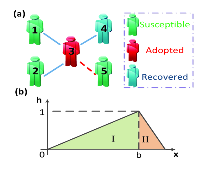
Figure 1: (a) Illustration of social contagions on complex networks. (b) Tent-like behavior adoption probability. Notations $b$ and $x$ indicate local trend imitation capacity and the ratio of adopted informants, respectively. In region I, the adoption probability increases with $x$. In region II, the adoption probability decreases with $x$.

2 Model Description

We here use a generalized susceptible-adopted-recovered (SAR) model [20, 21, 22] to describe behavior spreading in complex networks with $N$ nodes and a degree distribution $P(k)$. Figure 1(a) shows that at any given time each individual is in either a susceptible (S), adopted (A) or recovered (R) state. An individual in the susceptible state has not adopted the behavior. An individual in the adopted state adopts the behavior and exhibits or transmits it to susceptible neighbors. An individual in the recovered state abandons the behavior and no longer exhibits or transmits it.

To include the LTI effect in social contagions, we use a tent-like function $h(x,b)$ as the behavior adoption probability, defined as

$$h(x,b)=\left\{{\begin{array}[]{*{20}{c}}{\frac{x}{b},}&{~{}0<x\leq b},\\ {\frac{{1-x}}{{1-b}},}&{~{}b<x<1,}\end{array}}\right.$$ (1)

where $x$ is the ratio between an individual’s received information and its degree. The parameter $b$ is the LTI capacity of an individual. When $0<x\leq b$, i.e., region I in Fig. 1(b), the adoption probability increases with $x$. Thus region I is the promotion region. When $b<x<1$, i.e., region II in Fig. 1(b), the adoption probability decreases with $x$. Region II is the depression region. Small $b$ increases the LTI capacity, and when the value of $b$ is large, the LTI capacity decreases.

We initially randomly select a seed to be an adopter and allow the rest to remain susceptible. At each time step, every adopted individual $v$ transmits behavioral information to every susceptible neighbor with a probability $\lambda$. If a susceptible neighbor $u$ of $v$ receives the information, the cumulative pieces of information $m$ collected by $u$ increases by one, i.e., $m=m+1$. We disallow multi-transmission of information between individuals $u$ and $v$, i.e., only non-redundant information transmission is allowed. Individual $u$ becomes adopted with a probability $h(m/k,b)$, in which $k$ is the degree of individual $u$. Thus the system is non-Markovian. Every adopted individual abandons the behavior with a probability $\gamma$, and moves to the recovered state. The spreading dynamics terminate when all adopted individuals have moved to the recovered state.

3 Theoretical analysis

To describe our proposed model, we use Refs. [20, 29, 30] and develop a generalized edge-based compartmental theory. We define mathematical symbols $S(t)$, $A(t)$, and $R(t)$ as the fraction of individuals in the susceptible, adopted, and recovered states at time step $t$, respectively.

We assume that individual $u$ in the cavity state [31] receives behavioral information from adopted neighbors but does not transmit it further. We define $\theta(t)$ to be the probability that individual $v$ by time $t$ has not transmitted the behavioral information to individual $u$ along a randomly selected edge. By time $t$, an individual $u$ with degree $k$ has received $m$ pieces of behavioral information from different neighbors at probability

$$\phi_{m}(k,t)={k\choose m}[\theta(t)]^{k-m}[1-\theta(t)]^{m}.$$ (2)

Individual $u$, with degree $k$ and $m$ units of received information, remains susceptible with a probability $\prod\limits_{j=0}^{m}{[1-h(\frac{j}{k},b)]}$. We determine the probability that individual $u$ with degree $k$ has received $m$ units of information and by time $t$ is still in susceptible state with

$$S(k,t) =\sum\limits_{m=0}^{k}{{\phi_{m}}(k,t)\prod\limits_{j=0}^{m}{[1-h(\frac{j}{k},b)]}}$$ (3)

$$=\sum\limits_{m=0}^{\left\lfloor{bk}\right\rfloor}{{\phi_{m}}}(k,t)\prod\limits_{j=0}^{m}{[1-\frac{j}{{bk}}]}{\rm{}}+\sum\limits_{m=\left\lceil{bk}\right\rceil}^{k}{{\phi_{m}}}(k,t)\prod\limits_{j=0}^{\left\lceil{bk}\right\rceil}{[1-\frac{j}{{bk}}]}\prod\limits_{j=\left\lceil{bk}\right\rceil}^{m}{[1-\frac{{1-\frac{j}{k}}}{{1-b}}]}.$$

Considering all possible degrees $k$, we calculate the total ratio of susceptible individuals to be

$$S(t)=\sum\limits_{k}{P(k)S(k,t)}.$$ (4)

Neighbor $v$ of individual $u$ is either susceptible, adopted, or recovered, thus $\theta(t)$ can be divided, i.e.,

$$\theta(t)={\xi_{S}}(t)+{\xi_{A}}(t)+{\xi_{R}}(t),$$ (5)

where ${\xi_{S}}(t)$ [${\xi_{A}}(t)$, ${\xi_{R}}(t)$] is the probability that neighbor $v$ of individual $u$ is in the susceptible (adopted, recovered) state and has not transmitted the behavioral information to $u$ by time $t$.

When individual $v$ with degree $k^{\prime}$ is initially susceptible, they cannot transmit behavioral information to $u$, but can receive information from all $k^{\prime}-1$ neighbors except susceptible $u$. Thus we determine the probability that individual $v$ by time $t$ has received $m$ units of information to be

$$\phi_{m}(k^{\prime}-1,t)={k^{\prime}-1\choose m}[\theta(t)]^{k^{\prime}-m-1}[1-\theta(t)]^{m}.$$ (6)

Taking into consideratin all possible values of $m$, we determine the probability that individual $v$ with degree $k^{\prime}$ remains susceptible to be

$$\Theta(k^{\prime},t) =\sum\limits_{m=0}^{k^{\prime}-1}{{\phi_{m}}}(k^{\prime}-1,t)\prod\limits_{j=0}^{m}{[1-h(\frac{j}{{k^{\prime}}},b)]}$$ (7)

$$=\sum\limits_{m=0}^{\left\lfloor{bk^{\prime}}\right\rfloor}{{\phi_{m}}}(k^{\prime}-1,t)\prod\limits_{j=0}^{m}{[1-\frac{j}{{bk^{\prime}}}]}{\rm{}}+\sum\limits_{m=\left\lceil{bk^{\prime}}\right\rceil}^{k^{\prime}-1}{{\phi_{m}}}(k^{\prime}-1,t)\prod\limits_{j=0}^{\left\lceil{bk^{\prime}}\right\rceil}{[1-\frac{j}{{bk^{\prime}}}]}\prod\limits_{j=\left\lceil{bk^{\prime}}\right\rceil}^{m}{[1-\frac{{1-\frac{j}{{k^{\prime}}}}}{{1-b}}]}.$$

In an uncorrelated network, an edge connects an individual of degree $k^{\prime}$ with probability $k^{\prime}P(k^{\prime})/\langle k\rangle$, where $\langle k\rangle$ is the average degree. We obtain

$${\xi_{S}}(t)=\sum\limits_{k^{\prime}}{\frac{{k^{\prime}P(k^{\prime})}}{{\langle k\rangle}}}\Theta(k^{\prime},t).$$ (8)

If an adopted individual transmits behavioral information through an edge with probability $\lambda$, $\theta(t)$ does not fulfill the definition, and the decrease of the fraction of $\theta(t)$ equals $\lambda{\xi_{A}}(t)$, which is

$$\frac{{d\theta(t)}}{{dt}}=-\lambda{\xi_{A}}(t).$$ (9)

If an adopted individual does not transmit the behavioral information through any edge with probability $1-\lambda$ but moves into the recovered state with probability $\gamma$, ${\xi_{R}}(t)$ will consequently increase. We thus obtain

$$\frac{{d{\xi_{R}}(t)}}{{dt}}=\gamma(1-\lambda){\xi_{A}}(t).$$ (10)

Using Eqs. (9) and (10), and the initial conditions of $\theta(0)=1$ and ${\xi_{R}}(0)=0$, we get

$${\xi_{R}}(t)=\frac{{\gamma[1-\theta(t)](1-\lambda)}}{\lambda}.$$ (11)

Substituting ${\xi_{S}}(t)$, ${\xi_{A}}(t)$ and ${\xi_{R}}(t)$ of Eq. (5) into Eqs. (8), (9), and (11), respectively, we find the time evolution of $\theta(t)$ to be

$$\frac{{d\theta(t)}}{{dt}}=-\lambda[\theta(t)-\sum\limits_{k^{\prime}}{\frac{{k^{\prime}P(k^{\prime})}}{{\langle k\rangle}}\Theta(k^{\prime},t)}]+\gamma[1-\theta(t)](1-\lambda).$$ (12)

At each time step $t$, some susceptible individuals adopt the behavior and some adopted individuals move into the recovered state. Note that the growth of $A(t)$ is equivalent to the decrease of $S(t)$ minus the fraction of adopted individuals that with probability $\gamma$ enter the recovered state. Thus the time evolution of $A(t)$ is

$$\frac{{dA(t)}}{{dt}} =-\frac{{dS(t)}}{{dt}}-\gamma A(t)$$ (13)

$$=-\sum\limits_{k}{P(k)\frac{{dS(k,t)}}{{dt}}}-\gamma A(t),$$

where

$$\frac{{dS(k,t)}}{{dt}}=\sum\limits_{m=0}^{\left\lfloor{bk}\right\rfloor}{\Psi(t)}\prod\limits_{j=0}^{m}{[1-\frac{j}{{bk}}]}{\rm{}}+\sum\limits_{m=\left\lceil{bk}\right\rceil}^{k}{\Psi(t)}\prod\limits_{j=0}^{\left\lceil{bk}\right\rceil}{[1-\frac{j}{{bk}}]}\prod\limits_{j=\left\lceil{bk}\right\rceil}^{m}{[1-\frac{{1-\frac{j}{k}}}{{1-b}}]},$$ (14)

and

$$\Psi(t) =\frac{{d{\phi_{m}}(k,t)}}{{dt}}$$ (17)

$$=\left({\begin{array}[]{*{20}{c}}k\\ m\end{array}}\right)\left\{{(k^{\prime}-m-1){{[\theta(t)]}^{k^{\prime}-m-2}}{{[1-\theta(t)]}^{m}}-m{{[\theta(t)]}^{k^{\prime}-1-m}}{{[1-\theta(t)]}^{m}}}\right\}.$$

The time evolution of $R(t)$ is

$$\frac{{dR(t)}}{{dt}}=\gamma A(t).$$ (18)

Equations (2)–(4) and (12)–(13) describe social contagion in terms of LTI, and they can be used to compute the fraction of each state at any arbitrary time step. When $t\to\infty$, we find the final adoption size $R(\infty)$.

In the final state, we find that

$$\theta(\infty)=\sum\limits_{k^{\prime}}{\frac{{k^{\prime}P(k^{\prime})}}{{\langle k\rangle}}}\Theta(k^{\prime},\infty)+\frac{{\gamma[1-\theta(\infty)](1-\lambda)}}{\lambda}.$$ (19)

Note that $\theta(t)$ decreases with $t$ when adopted individuals continually transmit the behavioral information to neighbors. Thus when there is more than one stable fixed point in Eq. (19) only the maximum stable fixed point is physically meaningful. Inserting this value into Eqs. (2)–(4) gives us the steady value of the susceptible density $S(\infty)$ and the final behavior adoption size $R(\infty)$.

Numerically solving Eq. (20), we find that either (i) it has only two solutions for any value of $\lambda$ [see Fig. 2(a)], or (ii) it has either one or three solutions for different values of $\lambda$ [see Fig. 2(b)]. When (i) occurs, the trivial solution of Eq. (19) is $\theta(\infty)=1$ and there is no global behavior adoption. When global behavior occurs, Eq. (19) has a non-trivial solution $\theta(\infty)<1$. At the critical point, the equation

$$\begin{array}[]{l}g[\theta(\infty),b,\gamma,\lambda]=\sum\limits_{k^{\prime}=1}^{N-1}{\frac{{k^{\prime}P(k^{\prime})}}{{\langle k\rangle}}}\Theta(k^{\prime},\infty)+\frac{{\gamma[1-\theta(\infty)](1-\lambda)}}{\lambda}-\theta(\infty)\end{array}$$ (20)

is tangent to the horizontal axis at $\theta(\infty)=1$. Thus we find the critical condition of the general social contagion model to be

$$\frac{{dg}}{{d\theta(\infty)}}{|_{{\theta}(\infty)=1}}=0.$$ (21)

Using Eq. (21) we find the continuous critical information transmission probability to be

$${\lambda_{c}^{\rm II}}=\frac{\gamma}{{\Gamma+\gamma-1}},$$ (22)

where

$$\Gamma=\sum\limits_{k^{\prime}}{\frac{{k^{\prime}P(k^{\prime})}}{{\langle k\rangle}}}(k^{\prime}-1)h(\frac{1}{{k^{\prime}}},b).$$

Numerically solving Eqs. (19)–(22), we find $\lambda_{c}^{\rm II}$ to be a given adoption probability $h(x,b)$. Here $\lambda_{c}^{\rm II}$ is associated with adoption probability $h(x,b)$, recovery probability $\gamma$, degree distribution $P(k)$, and average degree $\langle k\rangle$.

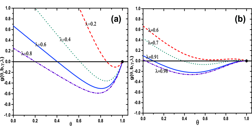
Figure 2: (Color online) Demonstration of graphical solutions of Eq. (20) for $b=0.1$ (a) and $b=0.9$ (b). The horizontal axis are colored black and the tangent points are denoted as black dots.

In the second scenario, Eq. (19) can have three solutions, and a saddle-node bifurcation can occur [see Fig. 2(b)]. Only the largest solution is valid because only that value can be achieved physically. Otherwise the fixed point is the valid solution. Changing $\lambda$ causes the physically meaningful stable solution of $\theta(\infty)$ to jump to an alternate value. A discontinuous growth pattern of $R(\infty)$ with $\lambda$ emerges, and solving Eqs. (19)–(22) gives us the critical transmission probability $\lambda^{\rm II}_{c}$ at which the discontinuity occurs. When $b=0.9$, for different values of $\lambda$ the function $g[\theta(\infty),b,\gamma,\lambda]$ is tangent to the horizontal axis at $\lambda^{\rm II}_{c}=0.91$. When $\lambda<\lambda^{\rm II}_{c}$, if there are three fixed points in Eq. (19), e.g., $\lambda=0.7$, the largest is the solution. When $\lambda=\lambda^{\rm II}_{c}$, the tangent point is the solution. When $\lambda>\lambda^{\rm II}_{c}$, e.g., $\lambda=0.98$, the only fixed point is the solution of Eq. (19), which abruptly drops to a small value from a large value at $\lambda=\lambda^{\rm II}_{c}$ and causes a discontinuous change in $R(\infty)$.

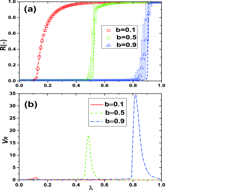
Figure 3: (Color online) Illustration of effects of dynamical parameter $b$ with arbitrary $\lambda$, where $b$ is the LTI capacity parameter. (a) Under different $b$, the increase manners of final adoption size change from continuity at small $b$ (e.g. $b=0.1$) to discontinuity at large $b$ (e.g. $b=0.5$), which embody the second-order and first-order phase transition. (b) $v_{R}$ numerically exhibits the fluctuation of $R(\infty)$ to intuitively emphasize the critical $\lambda_{c}^{\rm I}$ corresponding to the peak. The higher peak, the more abrupt the discontinuity of $R(\infty)$ is (see $b=0.1,0.5and0.9$).

For a given $P(k)$, $\lambda$, and $\gamma$ and using the analytical method similar to Eq. (22), we set $f(b)=\Gamma$ to be

$$f(b)=\sum\limits_{k^{\prime}}{\frac{{k^{\prime}P(k^{\prime})}}{{\langle k\rangle}}}(k^{\prime}-1)h(\frac{1}{{k^{\prime}}},b),$$ (23)

and

$$f(b)=\frac{\gamma+\lambda-\gamma\lambda}{\lambda}.$$ (24)

Using Eqs. (23) and (24) gives us the critical $b$ solution

$$b_{c}^{\rm II}=f^{-1}(\frac{\gamma+\lambda-\gamma\lambda}{\lambda}).$$ (25)

From this theoretical analysis and using non-redundant memory, the social contagion with LTI character displays first and second-order phase transitions.

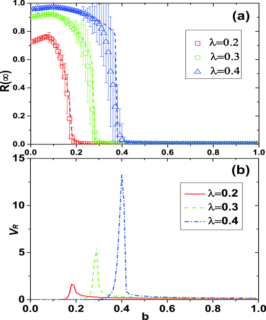
Figure 4: (Color online) Illustration of effects of dynamical parameter $\lambda$ with arbitrary $b$, where $\lambda$ is behavior transmission probability and $b$ is LTI capacity parameter. (a) Under different $\lambda$, the change pattern of $R(\infty)$ with $b$ shows a first increase and then a decrease. Ultimately, the $R(\infty)$ vanishes to zero. (b) To find the critical point where the $R(\infty)$ vanishes, $v_{R}$ is introduced here. Besides, the peaks of $v_{R}$ lines correspond to critical points, and the higher the peaks the sharper the jump to zero.

4 Numerical simulations

Extensive experiments have been performed on ER and SF, where the network size, mean degree, and recovered probability are $N=10^{4}$, ${\langle k\rangle}=10$, and $\gamma=1.0$, respectively. The relative variance $v_{R}$ is designed numerically to determine the size-dependent critical values $\lambda_{c}^{\rm II}$ and $b_{c}^{\rm II}$. The relative variance of $R(\infty)$[34] is defined as

$${v_{R}}=\frac{{\langle{{(R(\infty)-\langle R(\infty)\rangle)}^{2}}\rangle}}{{{{\langle R(\infty)\rangle}^{2}}}},$$ (26)

where $\langle...\rangle$ is the ensemble average. The value of $v_{R}$ shows the peaks (indicating phase transitions) of $R(\infty)$ when a dynamical parameter is varied. Thus we know that the $\lambda_{c}^{\rm II}$ and $b_{c}^{\rm II}$ correspond to the maximum $v_{R}$ under different values of $\lambda$ and $b$, respectively.

To study social contagions on ER networks, we examine the final behavior adoption size $R(\infty)$ as a function of the transmission probability $\lambda$ for different values of the LTI capacity parameter $b$ when $\gamma=1.0$. Figure 3(a) shows that a bifurcation analysis of Eq. (19) reveals that the LTI on adopted informants at different $b$ affects the type of phase transition. When the LTI capacity is strong, e.g., $b=0.1$, the system exhibits a second-order phase transition because a small $b$ value indicates that a low ratio of informants can cause massive behavior adoptions even when the transmission rate $\lambda$ is low. When the LTI capacity is weak, e.g., $b=0.5$ or 0.9, the system exhibits a first-order phase transition because a high $b$ value indicates that a high ratio of informants and low transmission rate $\lambda$ with a low probability of transmitting information does not substantially increase the informant ratio of susceptible individuals. When $b$ is high, the transmission rate $\lambda$ must exceed a critical point for there to be a massive information reception by many individuals that greatly increases the informant ratio of susceptible individuals, which results in an abrupt outbreak of behavior adoption.

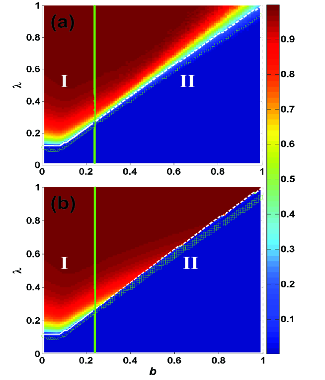
Figure 5: Dependance of $R(\infty)$ on $b$ and $\lambda$ on ER network. Color-coded values of $R(\infty)$ are obtained from numerical simulations (a) and theoretical solutions (b). Herein, the theoretical solutions are achieved through Eqs. (2)-(4) and (9)-(18). The parameter plain is divided into two regions by $b^{*}$ which is obtained from Eqs. (21), (22) and (25). In regions $I$, $R(\infty)$ shows a continuous increase and undergoes a second-order phase transition. In contrast, $R(\infty)$ exhibits a discontinuous increase and undergoes a first-order phase transition in region $II$. The solid white line from theoretical method and green circles from numerical simulation all represent the critical $\lambda_{c}^{\rm II}$ in region $I$. And the dashed white line from theoretical method and green rectangles from numerical simulation as well denote the the critical $\lambda_{c}^{\rm II}$ in region $II$.

We calculate the theoretical value of $\lambda_{c}^{\rm II}$ using Eqs. (19)–(21). To locate the numerical critical points, we examine $v_{R}$ shown in Fig. 3(b). Our theory coincides with these simulation results well, except when $\lambda$ is close to the critical information transmission probability. The deviations between our predictions and the simulations are caused by the finite-size effects of networks, and the strong dynamical correlations among the states of neighbors.

Figure 4 shows an analysis of $R(\infty)$ versus $b$ for different $\lambda$ values. For a given $\lambda$, $R(\infty)$ changes nonmonotonically with $\lambda$. In particular, $R(\infty)$ first increases with $b$ and then decreases discontinuously to zero. Thus there is an optimal $b_{o}$ value at which $R(\infty)$ reaches its maximum value. To explore the reason, given $\lambda$, when $b$ is smaller than the optimal $b$, LTI capacity is very strong and a lot of neighbors around the susceptible turn into informed state, leading to ever-increasing $R(\infty)$. When $b$ becomes greater, LTI capacity gradually decreases showing reduced capacity in informing neighbors, but $R(\infty)$ still keeps increasing until $b$ exceeds the optimal $b$. At the optimal $b$, the informing process enters in a balance status and the $R(\infty)$ also reaches the maximum. Gradually, when $b$ is greater than the optimal $b$, LTI capacity and informing capacity considerably degrade, leading to insufficient informed neighbors to effectively support further informing, so $R(\infty)$ enters in ever-declining status until zero. The critical point can be located by studying $v_{R}$ as shown Fig. 4(b). Again, our theory agree well with the numerical simulations.

Figure 5 shows a study of the phase transition plane $(\lambda,b)$. According to the type of phase transition, the parameter plane $(\lambda,b)$ is divided into two regions by the critical value of $b$ ($b^{*}=0.237$), which can be obtained using Eqs. (20) and (22). In region I, i.e., $(b\leq b^{*})$, $R(\infty)$ increases continuously and exhibits a second-order phase transition. In region II, i.e., $(b>b^{*})$, $R(\infty)$ increases discontinuously with $\lambda$ and exhibits a first-order phase transition. There is also a crossover in the phase transition. The numerical simulation generally agrees with theoretical solution.

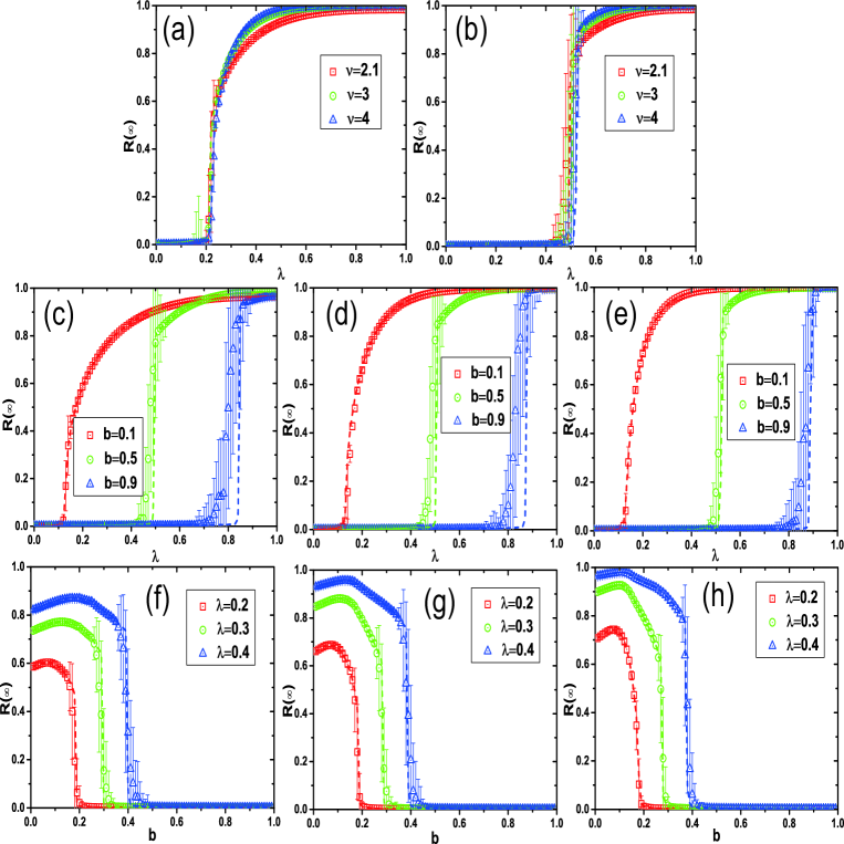
Figure 6: (Color online) Effect of network heterogeneity in social contagion dynamics. For scale-free network with mean degree $\langle k\rangle=10$ and network size $N=10000$, dependence of $R(\infty)$ on $b$, $v$, and $\lambda$ is explored under parameter values. Subgraph (a) and (b) demonstrate the impact on $R(\infty)$ of separate degree exponent $v$, respectively under $b=0.2$ and $0.5$. Then, subgraph (c), (d), and (e) exhibit the results of $b$ influencing $R(\infty)$, referring to degree exponent $v=2.1$, $3$, and $4$. Furthermore, for rigorousness, subgraph (f), (g), and (h) proceed to show the changes of $R(\infty)$ based on different transmission probability $\lambda$, also separately under $v=2.1$, $3$, and $4$. As expected, the theoretical solutions, denoted by dash line, perfectly coincide with numerical values, marked by symbols.

Figure 6 shows a study of the effects of the heterogeneity of degree distribution on social contagion. Here we focus on the SF network with different degree exponents $v$. We set the average degree and network size to be $\langle k\rangle=10$ and $N=10^{4}$, respectively. Figures 6(a) and 6(b) show that the heterogeneity of degree distribution does not change the type of phase transition when $b=0.2$ and $0.5$, respectively.

Figure 6(a) shows that when $b=0.2$ the increase of $R(\infty)$ exhibits a change from a discontinuous first-order to a continuous second-order phase transition, when $v$ rises from $2.1$ to $4$. Figure 6(b) shows, in contrast, when $b=0.5$, $R(\infty)$ increases and exhibits the same pattern of first-order phase transition at any $v$ value and jumps higher at the critical $\lambda_{c}^{\rm II}$ when $v=2.1$, $3$, and $4$. Figures 6(c)–6(e) show that when $v=2.1$, $v=3$, and $v=4$ increasing $b$ also changes the growth pattern of $R(\infty)$ from a second-order phase transition to a first-order, but that the final adoption size increases with $v$, i.e., the heterogeneous degree distribution does not impede the change in phase transition. Figures 6(f)–6(h) show that when $v=2.1$, $v=3$, and $v=4$ the transmission probability $\lambda$ influences the final range of $R(\infty)$ that increases the number of individuals when $v$ is higher. For all three values and under each $\lambda$ the optimal LTI capacity parameter $b$ that maximizes $R(\infty)$ appears, and the critical LTI capacity point of $b_{c}^{\rm II}$ reduces $R(\infty)$ to zero, even though a higher value of $v$ promotes a wider spreading of behavior information. A heterogeneous degree distribution always causes a change of phase transition as in (c)-(e) and of optimal and critical LTI capacity parameters as in (f)-(h). In addition, the theoretical solutions (dashed lines) agree with the numerical values (symbols) in all subsections of Fig. 6.

5 Conclusions

The local trend imitation (LTI) phenomenon is ubiquitous and strongly affects the dynamics of social contagions. We have proposed a social contagion model that uses a tent-like adoption function to systematically study the role of LTI. We use an edge-based compartmental theory to describe the model and find that the theoretical predictions agree with the numerical simulations. We also perform extensive numerical simulations on ER networks. We find that when the LTI capacity is weak the size of the final behavior adoption grows discontinuously, i.e., the system exhibits a first-order transition, but when the LTI capacity is strong the size of the final behavior adoption grows continuously, i.e., the system exhibits a second-order phase transition. Thus there is a crossover in the phase transition type. For a given probability of information transmission, there an optimal LTI capacity at which the final behavior adoption size is markedly increased. We also find that degree heterogeneity does not qualitatively alter these phenomena.

References

References

- [1] Watts D J and Dodds P S 2007 Journal of Consumer Research, 34 441.
- [2] Castellano C, Fortunato S and Fortunato S 2009 Rev. Mod. Phys. 81 0034.
- [3] Centola D 2011 Science 334 1269.
- [4] Gao L, Wang W, Pan L M, Tang M, and Zhang H F 2016 Sci. Rep. 6 38220.
- [5] Christakis N A and Fowler J H 2007 N. Engl. J. Med. 357 370.
- [6] Barrat A, Barthélemy M, and Vespignani A 2007 Dynamical Processes on Complex Networks (Cambridge: Cambridge University Press).
- [7] Pastor-Satorras R and Vespignani A 2001 Phys. Rev. Lett. 86 3200.
- [8] Wang W, Tang M, Yang H, Do Y, Lai Y C, and Lee G W 2014 Sci. Rep. 4 5097.
- [9] Shu P, Wang W, Tang M, Zhao P, and Zhang Y C. 2016 Chaos 26 063108.
- [10] Liu Q H, Wang W, Tang M, Zhou T, and Lai Y C 2017 Phys. Rev. E 95 042320.
- [11] Pastor-Satorras R, Castellano C, Mieghem P V and Vespignani A 2015 Rev. Mod. Phys. 87 925.
- [12] Porter M A and Gleeson J P 2014 arXiv:1403.7663v1.
- [13] Watts D J 2002 Proc. Natl. Acad. Sci. 99 5766.
- [14] Gleeson J P and Cahalane D J 2007 Phys. Rev. E 75 056103.
- [15] Dodds P S and Payne J L 2009 Phys. Rev. E 79 066115.
- [16] Gleeson J P 2008 Phys. Rev. E 77 046117.
- [17] Granovetter M 1973 Am. J. Sociol. 78 1360.
- [18] Dodds P S and Watts D J 2004. Phy. Rev. Lett. 92 218701.
- [19] Zheng M, Lü L and Zhao M 2013 Phys. Rev. E 88 012818.
- [20] Wang W, Tang M, Zhang H-F and Lai Y-C 2015 Phys. Rev. E 92 012820.
- [21] Wang W, Shu P, Zhu Y X, Tang M, and Zhang Y C 2015 Chaos 25 103102.
- [22] Wang W, Tang M, Shu P, and Wang Z 2016 New J. Phys. 18 013029.
- [23] Liu M X, Wang W, Liu Y, Tang M, Cai S M, and Zhang H F 2017 Phys. Rev. E 95 052306.
- [24] Leibenstein H 1976 Harvard University Press, Cambridge, MA
- [25] Simmel G. 1957 Am. J. Sociology 62 541.
- [26] Granovetter M, and Soong R. 1986 J. Econ. Behav. Organ. 7 83-99.
- [27] Dodds P S, Harris K D, Danforth C M 2013 Phys. Rev. Lett. 110 158701.
- [28] Catanzaro M, Boguna ’ M, Pastor-Satorras R 2005 Phys. Rev. E 71 027103.
- [29] Miller J C, Slim A C and Volz E M 2011 J. R. Soc. Interface. 10 1098.
- [30] Miller J C and Volz E M 2013 PLoS ONE 8 e69162.
- [31] Karrer B and Newman M E J 2010 Phys. Rev. E 82 016101.
- [32] Strogatz S H 1994 Nonlinear dynamics and chaos: with applications to physics, biology, chemistry and engineering (Westview, Boulder, CO).
- [33] P. Erdős and Rényi. 1959 Publ. Math. 6, 290.
- [34] Chen W, Schröder M, D’Souza M R 2014 Phys. Rev. Lett. 112 155701.