A Simple Algorithm for Computing a Cycle Separator

Abstract

We present a linear time algorithm for computing a cycle separator in a planar graph that is (arguably) simpler than previously known algorithms. Our algorithm builds on, and is somewhat similar to, previous algorithms for computing separators. In particular, the algorithm described by Klein and Mozes [KM17] is quite similar to ours. The main new ingredient is a specific layered decomposition of the planar graph constructed differently from previous BFS-based layerings.

1 Introduction

The planar separator theorem is a fundamental result in the study of planar graphs that has been used in many divide and conquer algorithms. The theorem guarantees for planar graphs the existence of $O(\sqrt{n})$ vertices whose removal breaks the graph into “small” pieces, connected components of size at most $\alpha n$ for a constant $\alpha$. For triangulated planar graphs, a stronger result is known – the separator is a simple cycle of length $O(\sqrt{n})$ whose inside and outside (in the planar embedding) each contains at most $\alpha n$ vertices.

The separator theorem was first proved by Ungar [Ung51] with a slightly weaker upper bound of $O(\sqrt{n}\log n)$. Lipton and Tarjan [LT79] showed how to compute, in linear time, a separator of size $O(\sqrt{n})$. Later, Miller [Mil86] described a linear time algorithm for computing a cycle separator.

In this paper, we describe a simple algorithm for computing a cycle separator. We believe the simplicity of our algorithms is comparable to that of the original algorithm of Lipton and Tarjan [LT79].

Existential proofs.

Alon et al.. [AST94] described an existential proof of the cycle separator theorem using a maximality condition.

Miller et al. [MTTV97] showed how to compute a planar separator in a planar graph if its circle packing realization is given (this proof was later simplified by Har-Peled [Har13]). In particular, the planar separator theorem is an easy consequence of the work of Paul Koebe [Koe36] (see [Har13] for details). A nice property of the proof of Miller et al. [MTTV97], is that it immediately implies the cycle separator theorem. Unfortunately, there is no finite algorithm for computing the circle packing realization of a planar graph – all known algorithms are iterative convergence algorithms. That is, the proof of Miller et al. is an existential proof.

Constructive proofs.

As mentioned above, Miller [Mil86] gave a linear time algorithm for computing the cycle separator. A somewhat different algorithm is also provided in the work of Klein et al. [KMS13], which computes the whole hierarchy of such separators in linear time. Fox-Epstein et al. [FMPS16] also provides an algorithm for computing a cycle separator in linear time.

This paper.

A simple cycle is a $\alpha$-separator if its inside and outside each contains at most $\left\lceil{\alpha\mathsf{f}}\right\rceil$ faces, where $\mathsf{f}$ is the number of faces of the graph. We present a linear time algorithm for computing a cycle $2/3$-separator – see Theorem 3.6. The algorithm is somewhat similar in spirit to the work of Fox-Epstein et al. [FMPS16]. A closer algorithm to ours is described by Klein and Mozes [KM17, Section 5.9]. The new algorithm is (arguably) slightly simpler than these previous versions.

The rest of the paper is composed of two section. In Section 2 we define some required basic concepts, and in Section 3 we describe the new algorithm.

2 Preliminaries

Let $G$ be a triangulated planar graph embedded in the plane, with vertex set $V$, edge set $E$, and face set $F$, and let $G^{*}=(V^{*},E^{*},F^{*})$ be the dual of $G$. A vertex $x\in V$ corresponds to a face $x^{*}\in F^{*}$, an edge $xy\in E$ to an edge $\left({xy}\right)^{*}\in E^{*}$, and a face $xyz\in F$ to a vertex $(xyz)^{*}\in V^{*}$. Because of the last correspondence, and since $G$ is triangulated, $G^{*}$ is $3$-regular: all its vertices have degree three. For any spanning tree $\mathsf{T}=(E_{\mathsf{T}},V_{\mathsf{T}})$ of $G$, the duals of the edges $E\setminus E_{\mathsf{T}}$ form a spanning tree of the dual graph $G^{*}$.

For any simple cycle $C$ in the embedding of $G$, the inside (resp., outside) of $C$, denoted by $\mathrm{in}\left({C}\right)$ (resp., $\mathrm{out}\left({C}\right)$), is the bounded (resp., unbounded) region of $\mathbb{R}^{2}\setminus C$. Each vertex of $V$ is inside, outside or on $C$. A face is inside (resp. outside) $C$ if its interior is a subset of $\mathrm{in}\left({C}\right)$ (resp. $\mathrm{out}\left({C}\right)$). It follows that each face of $G$ is either inside or outside $C$. If a face $\theta$ is inside $C$, then $C$ contains $\theta$.

Definition 2.1.

For a cycle $C$, and an $1/2\leq\alpha<1$, $C$ is an $\alpha$-cycle separator of a graph $G$, if the number of faces inside (resp. outside) $C$ is at most $\left\lceil{\alpha\cdot\mathsf{f}}\right\rceil$, where $\mathsf{f}=\left|{F}\right|$ is the number of faces of $G$.

For two cycles $C_{1}$ and $C_{2}$ of $G$, $C_{1}$ is inside $C_{2}$, denoted by $C_{1}\preceq C_{2}$, if $\mathrm{in}\left({C_{1}}\right)\subseteq\mathrm{in}\left({C_{2}}\right)$. For $C_{1}\preceq C_{2}$, a face is between $C_{1}$ and $C_{2}$, if it is inside $C_{2}$ and outside $C_{1}$.

Let $\gamma$ be a simple path or cycle in $G$. The length of $\gamma$, denoted by $\left|{\gamma}\right|$, is the number of edges of $\gamma$. If $\gamma$ is a path, and $x,y$ are vertices on $\gamma$, $\gamma[x,y]$ denotes the subpath of $\gamma$ between $x$ and $y$. For two internally disjoint paths $\gamma_{1}$ and $\gamma_{2}$, if the last vertex of $\gamma_{1}$ and the first vertex of $\gamma_{2}$ are identical, $\gamma_{1}\hskip 0.6pt\circ\hskip 0.6pt\gamma_{2}$ denotes the path or cycle obtained by their concatenation

3 The cycle separator theorem

Let $G=(V,E,F)$ be a triangulated planar graph embedded on the plane, and let $n=|V|$, and $\mathsf{f}=|F|$. In this section, we describe the linear time algorithm for computing a cycle separator of $G$.

Our construction is composed of three phases. First, we find a possibly long cycle separator $S$, by finding a spanning tree $\mathsf{T}$ of $G$, and a balanced edge separator $(uv)^{*}$ in its dual tree. The unique cycle in $\mathsf{T}\cup\{uv\}$ is guaranteed to be a (possibly long) cycle separator (Section 3.1). This part of the construction is similar to Lemma 2 of Lipton and Tarjan [LT79], and we include the details for completeness. Next, we build a nested sequence of cycles $C_{1}\preceq C_{2}\preceq\ldots\preceq C_{k}$ (Section 3.2). The specific construction of these cycles, which is guided by $S$, is the main new ingredient in the new algorithm. Finally, we consider the collection of cycles $C_{1},\ldots,C_{k}$ and $S$, and construct a few short cycles, such that one them is guaranteed to be a balanced separator (Section 3.3).

3.1 A possibly long cycle separator

We start by computing a balanced separator that, unfortunately, can be too long. For a BFS tree $\mathsf{T}$, we denote by $\pi\left({\mathsf{T},u}\right)$ the unique shortest path in $\mathsf{T}$ between the root of $\mathsf{T}$ and $u$.

Lemma 3.1 ([LT79]).

Given a triangulated planar graph $G$, one can compute, in linear time, a BFS tree $\mathsf{T}$ rooted at a vertex $\mathsf{r}$, and an edge $uv\in E\left({G}\right)$, such that:

1. the (shortest) paths $p_{u}=\pi\left({\mathsf{T},u}\right)$ and $p_{v}=\pi\left({\mathsf{T},v}\right)$ are edge disjoint,

2. the cycle $S=p_{u}\cup p_{v}\cup uv$ is a $2/3$-separator for $G$.

Proof:

Our proof is a slight modification of the one provided by Lipton and Tarjan [LT79], and we include it for the sake of completeness. Let $r^{\prime}\in V$ be any vertex, and let $\mathsf{T}=(V_{\mathsf{T}},E_{\mathsf{T}})$ be a BFS tree rooted at $r^{\prime}$. Also, let $D=E\setminus E_{\mathsf{T}}$, and note that the dual set of edges $D^{*}$ is a spanning tree of the dual $G^{*}$. Since $G$ is a triangulation, $D^{*}$ has maximum degree at most three. Thus, it contains an edge $(uv)^{*}$ whose removal leaves two connected components, $D^{*}_{in}$ and $D^{*}_{out}$, each with at most $\left\lceil{(2/3)\mathsf{f}}\right\rceil$ (dual) vertices, see Lemma A.1, where $\mathsf{f}=\left|{F}\right|$ is the number of faces of $G$. Let $D^{*}_{out}$ be the connected component that contains the dual of the outer face, and let $D^{*}_{in}$ be the other one.

Let $uv$ be the original edge that is dual of $(uv)^{*}$, and $S$ the unique cycle in $\mathsf{T}\cup\{uv\}$. The sets of faces inside and outside $S$, correspond to the vertex sets of $D^{*}_{in}$ and $D^{*}_{out}$, respectively. Thus, $S$ is a $2/3$-cycle separator.

Now, let $\mathsf{r}$ be the lowest common ancestor of $u$ and $v$ in $\mathsf{T}$. The cycle $S$ is composed of $p_{u}=\mathsf{T}[r,u]$, $p_{v}=\mathsf{T}[r,v]$ and the edge $uv$. Since $\mathsf{T}$ is a BFS tree, and $\mathsf{r}$ is an ancestor of $u$ and $v$, the paths $p_{u}$ and $p_{v}$ are shortest paths in $G$.

To get a BFS tree rooted at $\mathsf{r}$, one simply recompute the BFS tree starting from $\mathsf{r}$, where we include the edges of $p_{u}$ and $p_{v}$ in the newly computed BFS tree $\mathsf{T}$.  

For the rest of the algorithm, let $S$, $\mathsf{r}$, $uv$, $p_{u}$ and $p_{v}$ be as specified by Lemma 3.1. We emphasize that the graph is unweighted, $p_{u}$ and $p_{v}$ are shortest paths, and $u$ and $v$ are neighbors.

 

Figure 3.1: A graph and its BFS tree.

3.2 A nested sequence of short cycles

 

Figure 3.2: The region $P_{\leq{5}}$ and the associated outer cycle $C_{5}$.

Let $\mathsf{r}$ be the root node of the BFS tree $\mathsf{T}$ computed by Lemma 3.1. For $x\in V\left({G}\right)$, let $\ell\left({x}\right)$ be the distance in $\mathsf{T}$ of $x$ from the root $\mathsf{r}$. The level of a (triangular) face $\eta=xyz$ of $G$ is $\ell\left({\eta}\right)=\max\left({\ell\left({x}\right),\ell\left({y}\right),\ell\left({z}\right)}\right)$. In particular, a face $\eta=uvz\in F\left({G}\right)$ is $i$-close to $\mathsf{r}$ if $\ell\left({\eta}\right)\leq i$. The union of all $i$-close faces, form a region $P_{\leq{i}}$ in the plane. This region is simple, but it is not necessarily simply connected.

Let $\mathsf{h}=\max\left({\ell\left({u}\right),\ell\left({v}\right)}\right)$, and let $\psi\in\left\{{u,v}\right\}$ be the vertex realizing $\mathsf{h}$. We assume, for the sake of simplicity of exposition, that $\psi$ is one of the vertices of the outer face.

For $i<\mathsf{h}$, let ${\xi}_{i}$ be the outer connected component of $\partial P_{\leq{i}}$. This is a closed curve in the plane, with $\psi$ being outside it (as long as $i<\mathsf{h}$), and let $C_{i}$ be the corresponding cycle of edges in $G$ that corresponds to ${\xi}_{i}$. The resulting set of cycles is $C_{0},\ldots,C_{\mathsf{h}-1}$ (i.e., a cycle $C_{i}$ is empty if $i\geq\mathsf{h}$).

Lemma 3.2.

We have the following:

1. For any $i<\mathsf{h}$, the vertices of $C_{i}$ are all at distance $i$ from $\mathsf{r}$ in $\mathsf{T}$.

2. For any $i<\mathsf{h}$, the cycle $C_{i}$ is simple.

3. For any $i<j<\mathsf{h}$, the cycles $C_{i}$ and $C_{j}$ are vertex disjoint.

4. For $i<\mathsf{h}$, the cycle $C_{i}$ intersects the cycle $S$.

Proof:

(A) Consider a vertex $x$ in $G$ with $\ell\left({x}\right)<i$. As $\mathsf{T}$ is a BFS tree, we have that all the neighbors $y$ of $x$ in $G$, have $\ell\left({y}\right)\leq\ell\left({x}\right)+1\leq i$. Namely, all the triangles adjacent to $x$ are $i$-close, and the vertex $x$ is internal to the region $P_{\leq{i}}$, which implies that it can not appear in $C_{i}$.

(B) Since ${\xi}_{i}$ is the (closure) of the outer boundary of a connected set, the corresponding cycle of edges $C_{i}$ is a cycle in the graph. The bad case here is that a vertex $x$ is repeated in $C_{i}$ more than once. But then, $x$ is a cut vertex for $P_{\leq{i}}$ – removing it disconnects $P_{\leq{i}}$ – see Figure 3.3. Now, $\ell\left({x}\right)<i$ as the BFS from $\mathsf{r}$ must have passed through $x$ from one side of $P_{\leq{i}}$ to the other side. Arguing as in (A), implies that $x$ is internal to $P_{\leq{i}}$, which is a contradiction. Figure 3.3:

(C) is readily implied by (A).

(D) Indeed, $C_{i}$ must intersect the shortest path $p_{\psi}$ from $\mathsf{r}$ to $\psi$, and as this path is part of $S$, the claim follows.  

Computing the cycles $C_{i}$, for all $i$, can be done in linear time (without the explicit embedding of the edges of $G$). To this end, compute for all the (triangular) faces of $G$ their level. Next, mark all the edges between faces of level $i$ and $i+1$ as boundary edges forming $\partial P_{\leq{i}}$ – this yields a collection of cycles. To identify the right cycle, consider the shortest $p_{\psi}$ path between $\mathsf{r}$ and $\psi$. The cycle with a vertex that belongs to $p_{\psi}$ is the desired cycle $C_{i}$. Clearly, this can be done in linear time overall for all these cycles.

Lemma 3.3.

Let $\Delta>0$ be an arbitrary parameter. If $\mathsf{h}=\ell\left({\psi}\right)>\Delta$, then there exist an integer $i_{0}\in\left\llbracket\Delta\right\rrbracket$, such that $\left|{C_{i_{0}}}\right|>0$ and $\sum_{j\geq 0}\left|{C_{i_{0}+j\Delta}}\right|\leq n/\Delta$, where $\left|{C_{k}}\right|$ denotes the number of vertices of $C_{k}$.

Proof:

Setting $g(i)=\sum_{j\geq 0}\left|{C_{i+j\Delta}}\right|$. By Lemma 3.2 (D), $g(i)>0$, for $i=0,\ldots,\Delta-1$. We have

$$\sum_{i=0}^{\Delta-1}g(i)\leq\sum_{i=0}^{\Delta-1}\sum_{j\geq 0}\left|{C_{i+j\Delta}}\right|=\sum_{k\geq 0}^{\mathsf{h}-1}\left|{C_{k}}\right|\leq|V\left({G}\right)|\leq n,$$

as the cycles $C_{0},C_{1},\ldots,C_{\mathsf{h}-1}$ are disjoint. As such, there must be an index $i=i_{0}$ of the first summation that does not exceed the average.  

3.3 Constructing the cycle separator

3.3.1 The algorithm

Let $\Delta=\Theta(\sqrt{n})$ be a parameter to be specified shortly. Let $S$ be a $2/3$-cycle separator, and $\mathsf{r}$, $u$, $v$, $p_{u}$, and $p_{v}$ as specified by Lemma 3.1. If $\left|{S}\right|\leq 2\Delta$ then this is the desired a short cycle separator. So, assume that $\mathsf{h}\geq|{S}|/2>\Delta.$

For $j\geq 0$, let $\alpha_{j}=i_{0}+(j-1)\Delta$ be the index of the $j$th cycle in the small “ladder” of Lemma 3.3. Since $\mathsf{h}>\Delta$ and by Lemma 3.2 (D), the cycles $C_{i_{0}}=C_{\alpha_{0}}$ of the ladder intersects $S$. In particular, let $D_{j}=C_{\alpha_{j}}$, for $j=1,\ldots,k-1$, be the $j$th nested cycles of this light ladder that intersects $S$. Specifically, let $k$ the minimum value such that $\alpha_{k}\geq\mathsf{h}$. Let $D_{0}$ be the trivial cycle formed by the root vertex $\mathsf{r}$. Similarly, let $D_{k}$ be the trivial cycle formed only by the vertex $\psi$, such that its interior contains the whole graph.

For $j=0,\ldots,k$, let $\mathsf{f}_{j}$ be the number of faces in the interior of $D_{j}$. If for some $j$, we have that $\left\lfloor{\mathsf{f}/3}\right\rfloor\leq\mathsf{f}_{j}\leq\left\lceil{(2/3)\mathsf{f}}\right\rceil$, then $D_{j}$ is the desired separator, as its length is at most $n/\Delta$ by Lemma 3.2, where $\mathsf{f}$ is the number of faces of $G$.

Otherwise, there must be an index $i$, such that $\mathsf{f}_{i}<\mathsf{f}/3$, and $\mathsf{f}_{i+1}>(2/3)\mathsf{f}$. Assume, for the sake of simplicity of exposition that $0<i<k-1$ (the cases that $i=0$ or $i=k-1$ are degenerate and can be handled in a similar fashion to what follows).

  

Figure 3.4:

Consider the “heavy” ring $R$ bounded by the two of the nested cycles $D_{i+1}$ and $D_{i}$, see Figure 3.4.

Observation 3.4.

By Lemma 3.2, the cycles $D_{i}$ and $D_{i+1}$ each intersects $S$ in two vertices exactly. And $D_{i}$ is nested inside $D_{i+1}$.

Let $I_{i}$ and $O_{i}$ the portions of $D_{i}$ inside and outside $S$, respectively (define $I_{i+1}$ and $O_{i+1}$ similarly). Let $p_{i}$ and $q_{i}$ (resp., $p_{i+1}$ and $q_{i+1}$) be the endpoints of $I_{i}$ (resp., $I_{i+1}$), such that $p_{i}$ is adjacent to $p_{i+1}$ along $S$. We can now partition $R$ into two cycles $R_{1}$ and $R_{2}$. The region $R_{1}$ is bounded by the cycle formed by $J_{1}=S[q_{i},q_{i+1}]\hskip 0.6pt\circ\hskip 0.6ptI_{i+1}\hskip 0.6pt\circ\hskip 0.6ptS[p_{i+1},p_{i}]\hskip 0.6pt\circ\hskip 0.6ptI_{i}$. The region $R_{2}$ is bounded by the cycle formed by $J_{2}=S[q_{i},q_{i+1}]\hskip 0.6pt\circ\hskip 0.6ptO_{i+1}\hskip 0.6pt\circ\hskip 0.6ptS[p_{i+1},p_{i}]\hskip 0.6pt\circ\hskip 0.6ptO_{i},$ see Figure 3.5. We have that $\left|{J_{1}}\right|\leq\left|{D_{i}}\right|+\left|{D_{i+1}}\right|+2\Delta\leq n/\Delta+2\Delta,$ by Lemma 3.3. In particular, if $\mathsf{f}(R_{1})\geq\mathsf{f}/3$, then $J_{1}$ is the desired cycle separator, since $\mathsf{f}(R_{1})\leq\mathsf{f}(S)\leq\left\lceil{(2/3)\mathsf{f}}\right\rceil$. Figure 3.5:

Similarly, if $\mathsf{f}(R_{2})\geq\mathsf{f}/3$, then $J_{2}$ is the desired cycle separator, since $\mathsf{f}(R_{2})\leq\mathsf{f}-\mathsf{f}(S)\leq\left\lceil{(2/3)\mathsf{f}}\right\rceil.$

Otherwise, the algorithm returns the cycle $K$ formed by $O_{i}\hskip 0.6pt\circ\hskip 0.6ptS[q_{i},q_{i+1}]\hskip 0.6pt\circ\hskip 0.6ptI_{i+1}\hskip 0.6pt\circ\hskip 0.6ptS[p_{i+1},p_{i}]$ as the desired separator.

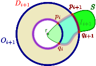
Figure 3.6:

3.3.2 Analysis

Lemma 3.5.

Assume that $\mathsf{f}(R_{1})<\mathsf{f}/3$ and $\mathsf{f}(R_{2})<\mathsf{f}/3$. Consider the region $Z$, formed by the union of the interior of $D_{i}$, together with the interior of $R_{1}$. Its boundary, is the cycle $K$ formed by $O_{i}\hskip 0.6pt\circ\hskip 0.6ptS[q_{i},q_{i+1}]\hskip 0.6pt\circ\hskip 0.6ptI_{i+1}\hskip 0.6pt\circ\hskip 0.6ptS[p_{i+1},p_{i}],$ see Figure 3.6. The cycle $K$ is a $2/3$-cycle separator with $n/\Delta+2\Delta$ edges.

Proof:

We have the following: (i) $\mathsf{f}_{i}<\mathsf{f}/3$, (ii) $\mathsf{f}_{i}+\mathsf{f}(R_{1})+\mathsf{f}(R_{2})=\mathsf{f}_{i+1}>(2/3)\mathsf{f}$, (iii) $\mathsf{f}(R_{1})<\mathsf{f}/3$, and (iv) $\mathsf{f}(R_{2})<\mathsf{f}/3$. Assume that $\mathsf{f}_{i}+\mathsf{f}(R_{1})<\mathsf{f}/3$. But then $\mathsf{f}_{i+1}=\mathsf{f}_{i}+\mathsf{f}(R_{1})+\mathsf{f}(R_{2})<(2/3)\mathsf{f}$, which is impossible. The region $Z$ bounded by $K$ contains $\mathsf{f}_{i}+\mathsf{f}(R_{1})$ faces, and we have $\mathsf{f}/3<\mathsf{f}_{i}+\mathsf{f}(R_{1})<(2/3)\mathsf{f}$, which implies the separator property.

As for the length of $K$, observe that $\left|{K}\right|\leq\left|{D_{i}}\right|+\left|{D_{i+1}}\right|+\left|{S[p_{i},p_{i+1}]}\right|+\left|{S[q_{i},q_{i+1}]}\right|\leq n/\Delta+2\Delta,$ by Lemma 3.3.  

Theorem 3.6.

Given an embedded triangulated planar graph $G$ with $n$ vertices and $\mathsf{f}$ faces, one can compute, in linear time, a simple cycle $K$ that is a $2/3$-separator of $G$. The cycle $K$ has at most $O(1)+\sqrt{8n}$ edges.

This cycle $K$ also $2/3$-separates the vertices of $G$ – namely, there are at most ${(2/3)n}$ vertices of $G$ on each side of it.

Proof:

The construction is described above. As for the length of $K$, set $\Delta=\left\lceil{\bigl{.}\smash{\sqrt{n/2}}\,}\right\rceil$. By Lemma 3.5, we have $\left|{K}\right|\leq 2\Delta+n/\Delta\leq O(1)+\sqrt{2n}+{\sqrt{2n}}\leq O(1)+{\sqrt{8n}}.$ (The separator cycle is even shorter if one of the other cases described above happens.)

As for the running time, observe that the algorithm runs BFS on the graph several times, identify the edges that form the relevant cycles. Count the number of faces inside these cycles, and finally counts the number of edges in $R_{1}$ and $R_{2}$. Clearly, all this work (with a careful implementation) can be done in linear time.

The second claim follows from a standard argument, see Lemma 3.7 (C) below for details.  

3.4 From faces separation to vertices separation

Lemma 3.7.

1. A simple planar graph $G$ with $n$ vertices has at most $3n-6$ edges and at most $2n-4$ faces. A triangulation has exactly $3n-6$ edges and $2n-4$ faces.

2. Let $G$ be a triangulated planar graph and let $C$ be a simple cycle in it. Then, there are exactly $(\mathsf{f}(C)-\left|{C}\right|)/2+1$ vertices in the interior of $C$, where $\mathsf{f}(C)$ denotes the number of faces of $G$ in the interior of $C$.

3. A simple cycle $C$ in a triangulated graph $G$ that has at most $\left\lceil{(2/3)\mathsf{f}}\right\rceil$ faces in its interior, contains at most $(2/3)n$ vertices in its interior, where $n$ and $\mathsf{f}$ are the number of vertices and faces of $G$, respectively.

Proof:

(A) is an immediate consequence of Euler’s formula.

(B) Let $n^{\prime}$ be the number of vertices of $G$ in or on $C$ – delete the portion of $G$ outside $C$, and add a vertex $v$ to $G$ outside $C$, and connect it to all the vertices of $C$. The resulting graph is a triangulation with $n^{\prime}+1$ vertices, and $2(n^{\prime}+1)-4=2n^{\prime}-2$ triangles, by part (A). This counts $\left|{C}\right|$ triangles that were created by the addition of $v$. As such, $\mathsf{f}(C)=2n^{\prime}-2-\left|{C}\right|$ $\implies$ $n^{\prime}=\mathsf{f}(C)/2+1+\left|{C}\right|/2$. The number of vertices inside $C$ is $n^{\prime}-\left|{C}\right|=(\mathsf{f}(C)-\left|{C}\right|)/2+1$.

(C) Part (B) implies that number of vertices inside the region formed by the cycle $C$ is

$$(\mathsf{f}(C)-\left|{C}\right|)/2+1 \leq(\left\lceil{(2/3)\mathsf{f}}\right\rceil-\left|{C}\right|)/2+1=(\left\lceil{(2/3)(2n-4)}\right\rceil-\left|{C}\right|)/2+1$$

$$\leq\frac{(2/3)(2n-4)+1-\left|{C}\right|}{2}+1\leq\frac{2}{3}n,$$

as claimed.  

Appendix A Balanced edge separator in a low-degree tree

The following lemma is well known, and we provide a proof for the sake of completeness.

Lemma A.1.

Let $\mathsf{T}$ be a tree with $n$ vertices, with maximum degree $d\geq 2$. Then, there exists an edge whose removal break $\mathsf{T}$ into two trees, each with at most $\left\lceil{(1-1/d)n}\right\rceil$ vertices. This edge can be computed in linear time.

Proof:

Let $v_{1}$ be an arbitrary vertex of $\mathsf{T}$, and root $\mathsf{T}$ at $v_{1}$. For a vertex $v$ of $\mathsf{T}$ let $n(v)$ denote the number of nodes in its subtree – this quantity can be precomputed, in linear time, for all the vertices in the tree using BFS.

In the $i$th step, $v_{i+1}$ be the child of $v_{i}$ with maximum number of vertices in its subtree. If $n(v_{i+1})\leq\left\lceil{(1-1/d)n}\right\rceil$, then the algorithm outputs the edge $xy$ as the desired edge separator, where $x=v_{i}$ and $y=v_{i+1}$. Otherwise, the algorithm continues the walk down to $v_{i+1}$. Since the tree is finite, the algorithm stops and output an edge.

Assume, for the sake of contradiction, that $n(y)<{n/d}$. But then, $x$ has at most $d(x)-1\leq d-1$ children (in the rooted tree), each one of them has at most $n(y)$ nodes (since $y$ was the “heaviest” child). As such, we have $n(x)\leq 1+(d-1)n(y)<1+(d-1){n/d}\leq\left\lceil{(1-1/d)n}\right\rceil$ if $d$ does not divides $n$. If $d$ divides $n$ then $n(x)\leq 1+(d-1)n(y)\leq 1+(d-1)(n/d-1)=((d-1)/d)n+2-d\leq\left\lceil{(1-1/d)n}\right\rceil.$

Namely, the algorithm would have stopped at $x$, and not continue to $y$, a contradiction.

As such, $n/d\leq n(y)\leq\left\lceil{(1-1/d)n}\right\rceil$. But this implies that $xy$ is the desired edge separator.

References

- [AST94] N. Alon, P. Seymour, and R. Thomas. Planar separators. SIAM J. Discrete Math., 2(7):184–193, 1994.
- [FMPS16] E. Fox-Epstein, S. Mozes, P. M. Phothilimthana, and C. Sommer. Short and simple cycle separators in planar graphs. ACM Journal of Experimental Algorithmics, 21(1):2.2:1–2.2:24, 2016.
- [Har13] S. Har-Peled. A simple proof of the existence of a planar separator. ArXiv e-prints, April 2013.
- [KM17] P.N. Klein and S. Mozes. Optimization algorithms for planar graphs. http://planarity.org, 2017. Book draft.
- [KMS13] P. N. Klein, S. Mozes, and C. Sommer. Structured recursive separator decompositions for planar graphs in linear time. In Proc. 45th Annu. ACM Sympos. Theory Comput. (STOC), pages 505–514, 2013.
- [Koe36] P. Koebe. Kontaktprobleme der konformen Abbildung. Ber. Verh. Sächs. Akademie der Wissenschaften Leipzig, Math.-Phys. Klasse, 88:141–164, 1936.
- [LT79] R. J. Lipton and R. E. Tarjan. A separator theorem for planar graphs. SIAM J. Appl. Math., 36:177–189, 1979.
- [Mil86] G. L. Miller. Finding small simple cycle separators for 2-connected planar graphs. J. Comput. Sys. Sci., 32(3):265–279, 1986.
- [MTTV97] G. L. Miller, S. H. Teng, W. P. Thurston, and S. A. Vavasis. Separators for sphere-packings and nearest neighbor graphs. J. Assoc. Comput. Mach., 44(1):1–29, 1997.
- [Ung51] P. Ungar. A theorem on planar graphs. J. London Math. Soc., 26:256–262, 1951.