Strong Convergence of Integrators for Nonequilibrium Langevin Dynamics

Abstract.

Several numerical schemes are proposed for the solution of Nonequilibrium Langevin Dynamics (NELD), and the rate of convergence is analyzed. Due to the special deforming boundary conditions used, care must be taken when using standard stochastic integration schemes, and we demonstrate a loss of convergence for a naive implementation. We then present several first and second order schemes, in the sense of strong convergence.

1. Introduction

Nonequilibrium molecular dynamics techniques are employed in the study of microscopic systems undergoing steady, nonconstant flow, for example, in the study of polymer melts. A wide range of dynamics, including both deterministic and stochastic equations have been proposed for such simulations [4, 12].

We examine the rates of strong convergence of several numerical methods for the simulation of Nonequilibrium Langevin Dynamics (NELD) [11, 12, 3]. Let $\mathbf{q},\mathbf{p}\in\mathbb{R}^{3N}$ denote the positions and velocities of a set of particles, then NELD is given by

$$\begin{split}d\mathbf{q}&=\mathbf{p}\,dt\\ d\mathbf{p}&=(-\textsc{$\nabla E$}(\mathbf{q})-\gamma(\mathbf{p}-A\mathbf{q})+A\mathbf{p})\,dt+\sigma\,dW\end{split}$$ (1)

where $-\nabla E(\mathbf{q})$ are the interparticle forces, $W$ is a standard $3N$-dimensional Brownian motion, $\sigma$ and $\gamma$ are scalar constants satisfying the fluctuation-dissipation relation

$$\begin{split}\gamma&=\frac{1}{2}\sigma^{2}\beta\end{split}$$ (2)

where $\beta=\frac{1}{k_{B}T}$ is the inverse temperature, and $A\in\mathbb{R}^{3N\times 3N}$ is trace-free block diagonal linear background flow matrix. The diagonal entries of $A$ are identical $3\times 3$ trace-free diagonal matrices, corresponding to the macroscale background flow $A=\nabla\mathbf{u}.$

To simulate the bulk motion of particles with a mean background flow $A,$ specialized periodic boundary conditions are employed, in particular, a particle with the coordinates $(\mathbf{q},\mathbf{p})$ has periodic images at $(\mathbf{q}+L_{t}\mathbf{n},\mathbf{p}+AL_{t}\mathbf{n})$, where $L_{t}:[0,\infty)\rightarrow\mathbb{R}^{3N\times 3N}$ is a block diagonal matrix whose $3\times 3$ identical blocks denote the matrix of lattice basis vectors at time $t$ and $\mathbf{n}\in\mathbb{Z}^{3N}.$ The images of a single particle do not have the same velocity, rather they are consistent with the mean flow, and this in turn implies that the periodic lattice generated by $L_{t}$ deforms with the flow. Care is needed to ensure that the lattice does not become degenerately deformed where the minimum replica distance goes to zero. Techniques have been developed in the papers [9, 8, 2, 6] which choose initial lattice vectors $L_{0}$ such that the minimum replica distance in the lattice stays bounded away from zero, and the simulation box is remapped so that the geometry stays regular. We will consider the Generalized Kraynik-Reinelt (GenKR) boundary conditions developed in [2, 6], which can handle general three-dimensional incompressible flows.

In this paper, we will focus on the strong convergence properties of certain common stochastic integrators applied to NELD, seeing how the periodic boundary conditions interact with the convergence. In particular, we will see that a naive implementation of certain standard schemes show a breakdown in convergence due to the interaction of the integrator with the GenKR boundary conditions. We will then develop schemes that avoid this convergence problems and compute the order of convergence by using the Ito-Taylor expansion. Several standard first and second order schemes will demonstrated numerically and analytically.

2. Ito-Taylor expansion of the nonequilibrium Langevin dynamics

In this section, we compute the Ito-Taylor expansion for the NELD up to second order, which will be used in the error analysis of the numerical integrators. We also set the notation for the application of boundary conditions as the motion of the replicas plays an important role in the analysis of the numerical schemes.

2.1. Review of the Ito-Taylor expansion

We express the NELD (1) in integral form,

$$\begin{split}X(t)=X(t_{0})+\int_{t_{0}}^{t}\textsc{C}(X(s))\,ds+\int_{t_{0}}^{t}\Sigma\,dW(s)\end{split}$$ (3)

where

$$C\left(\begin{bmatrix}\mathbf{q}\\ \mathbf{p}\end{bmatrix}\right)=\begin{bmatrix}\mathbf{p}\\ -\nabla E(\mathbf{q})-\gamma(\mathbf{p}-A\mathbf{q})+A\mathbf{p}\end{bmatrix}\qquad\Sigma=\begin{bmatrix}0&0\\ 0&\sigma I\end{bmatrix}.$$

The Ito formula for a scalar-valued function $G(X(t))$ of the solution $X(t)$ is given by

$$\begin{split}G(X(t))=G(X(t_{0}))+\int_{t_{0}}^{t}L^{0}G(X(s))\,ds+\int_{t_{0}}^{t}L^{1}G(X(s))\,dW(s)\end{split}$$ (4)

where the operators $L^{0}$ and $L^{1}$ are given by:

$$\begin{split}L^{0}&=\textsc{C}\cdot\nabla_{x}+\frac{1}{2}\Sigma\Sigma^{T}:\nabla_{x}^{2},\quad L^{1}=\Sigma\nabla_{x}\,.\end{split}$$ (5)

Over a small time interval $\Delta t:=t-t_{0},$ we apply the Ito formula to equation (3) and expand up to second order, noting that several terms cancel due to the form of $C$ and $\Sigma$, arriving at

$$\begin{split}X(t)&=X(t_{0})+\textsc{C}(X(t_{0}))\int_{t_{0}}^{t}ds+\Sigma\int_{t_{0}}^{t}dW(s)+L^{0}\textsc{C}(X(t_{0}))\int_{t_{0}}^{t}\int_{t_{0}}^{s}du\,ds\\ &\quad+L^{1}\textsc{C}(X(t_{0}))\int_{t_{0}}^{t}\int_{t_{0}}^{s}dW(u)\,ds+R\end{split}$$ (6)

where the remainder of order O($\Delta t^{5/2}$) term is given by

$$\begin{split}R&=\int_{t_{0}}^{t}\int_{t_{0}}^{s}\int_{t_{0}}^{u}L^{1}L^{0}C(X(v))\,dW(v)\,du\,ds+\int_{t_{0}}^{t}\int_{t_{0}}^{s}\int_{t_{0}}^{u}L^{0}L^{0}C(X(v))\,dv\,du\,ds.\end{split}$$ (7)

We recall the following facts about the covariance of $W(t)$ and its integral, which are useful in developing numerical schemes [7]:

$$\begin{split}\mathbb{E}(W_{i}(s)W_{j}(s^{^{\prime}}))&=\delta_{ij}\min(s,s^{^{\prime}})\\ \mathbb{E}[(W_{i}(s)-W_{i}(s^{^{\prime}}))(W_{j}(s)-W_{j}(s^{^{\prime}}))]&=\delta_{ij}\Delta t\\ \mathbb{E}\left[(W_{i}(t+\Delta t)-W_{i}(t))\int_{t}^{t+\Delta t}(W_{j}(s)-W_{j}(t))\,ds\right]&=\frac{1}{2}\delta_{ij}\Delta t^{2}\\ \mathbb{E}\left[\int_{t}^{t+\Delta t}(W_{i}(s)-W_{i}(t))\,ds\int_{t}^{t+\Delta t}(W_{j}(s)-W_{j}(t))\,ds\right]&=\frac{1}{3}\delta_{ij}\Delta t^{3}\end{split}$$ (8)

Therefore, truncating the expansion of NELD to second order and letting $(\mathbf{q},\mathbf{p})$ denote the coordinates at time $t_{0},$ we arrive at

$$\begin{split}\begin{bmatrix}\mathbf{q}(t)\\ \mathbf{p}(t)\end{bmatrix}&=\begin{bmatrix}\mathbf{q}\\ \mathbf{p}\end{bmatrix}+\begin{bmatrix}\mathbf{p}\\ \textsc{F}(\mathbf{p},\mathbf{q})\end{bmatrix}\Delta t+\Delta t^{1/2}\begin{bmatrix}0&0\\ 0&\sigma I\end{bmatrix}\bm{\eta}\\ &\quad+\begin{bmatrix}\textsc{F}(\mathbf{p},\mathbf{q})\\ (-\textsc{$\nabla^{2}E$}(\mathbf{q})+\gamma A)\mathbf{p}+(A-\gamma I)\textsc{F}(\mathbf{p},\mathbf{q})\end{bmatrix}\frac{\Delta t^{2}}{2}\\ &\quad+\sigma\Delta t^{3/2}\begin{bmatrix}0&I\\ 0&(A-\gamma I)\\ \end{bmatrix}\left(\frac{1}{2}\bm{\eta}+\frac{1}{2\sqrt{3}}\bm{\zeta}\right)+\textsc{O}(\Delta t^{5/2})\end{split}$$ (9)

where $\textsc{F}(\mathbf{p},\mathbf{q})=-\textsc{$\nabla E$}(\mathbf{q})-\gamma(\mathbf{p}-A\mathbf{q})+A\mathbf{p}$ and where

$$\begin{split}\bm{\eta}&=\frac{W(t)-W(t_{0})}{\Delta t},\\ \bm{\zeta}&=\frac{2\sqrt{3}}{\Delta t^{3/2}}\int_{t_{0}}^{t}\left(W(s)-W(t_{0})\right)\,ds\,-\,\sqrt{3}\,\bm{\eta}.\end{split}$$

Note the scaling of stochastic terms has been chosen so that $\bm{\eta},\bm{\zeta}\sim\mathcal{N}(0,1)$ are independent Gaussian random variables.

2.2. Nonequilibrium Boundary Conditions

When analyzing the truncation error for the scheme, it is important to account for the nonequilibrium periodic boundary conditions, particularly the fact that replicas do not all have the same velocity. A particle with coordinates $(\mathbf{q},\mathbf{p})$ has periodic images at $(\mathbf{q}+L_{t}\mathbf{n},\mathbf{p}+AL_{t}\mathbf{n}).$ The NELD equations are invariant under a translation of the system by choosing new $\mathbf{n}.$ In particular, $d\mathbf{q}=\mathbf{p}\,dt$ holds for all particle images, so that

$$\frac{d}{dt}(\mathbf{q}+L_{t}\mathbf{n})=\mathbf{p}+AL_{t}\mathbf{n}$$

which imply that the simulation box deforms with the flow, $\frac{d}{dt}L_{t}=AL_{t}$ with a solution $L_{t}=\exp(At)L_{0}$.

During a simulation step, one or more particles can leave the simulation box, whereupon they are remapped in accordance to the periodic boundary conditions. This can also be viewed as no longer tracking the position of the particles that started at $(\mathbf{q},\mathbf{p}),$ but tracking the particles at $(\mathbf{q}+L_{t}\mathbf{n},\mathbf{p}+AL_{t}\mathbf{n})$ for some $\mathbf{n}\in\mathbb{Z}^{3N}.$ We show in the following that the timing of applying the periodic boundary conditions affects the rate of convergence for the numerical scheme, in fact, reducing the strong rate of convergence below first order for a pair of schemes. When computing the local truncation error, we compare the final position after the numerical step and periodic remapping with the Taylor-Ito expansion of the corresponding replica, which may have started outside the simulation box. That is, if we are now tracking the particle at $(\mathbf{q}(t)+L_{t}\mathbf{n},\mathbf{p}(t)+AL_{t}\mathbf{n}),$ we compare with the particle that started at $(\mathbf{q}(t_{0})+L_{t_{0}}\mathbf{n},\mathbf{p}(t_{0})+AL_{t_{0}}\mathbf{n}).$ We note that the Taylor-Ito expansion will now have terms from the deformed lattice vectors,

$$\mathbf{q}(t)+L_{t}\mathbf{n}=\mathbf{q}(t)+L_{t_{0}}\mathbf{n}+\Delta tAL_{t_{0}}\mathbf{n}+\frac{1}{2}\Delta t^{2}A^{2}L_{t_{0}}\mathbf{n}+O(\Delta t^{3}),$$

with a similar expression for $\mathbf{p}(t)+AL_{t}\mathbf{n}.$

3. Strong Convergence and a Numerical Experiments

For a stochastic process, there are several notions of convergence one can consider, including strong convergence, weak convergence, or convergence of the dynamics to an invariant measure. In the following, we consider strong convergence of the proposed numerical schemes. Given a stochastic process $X(t),$ we say that the numerical method generating $X_{h}(t)$ has strong order of convergence $r$ if

$$\mathbb{E}(|X(t)-X_{h}(t)|)\leq Ch^{r}$$

for some $C>0$ and all sufficiently small $h>0.$

For each of the described algorithms, we perform a benchmark test to numerically compute the strong rate of convergence. For each time, we numerically estimate the rate of convergence in the $\ell^{2}$ norm of both the position $\mathbf{q}$ and momentum $\mathbf{p},$ and in each case the convergence is observed to behave similarly in $\mathbf{q}$ and $\mathbf{p}.$ We simulate a system of $1728$ particles, having the Weeks-Chandler-Anderson (WCA) interparticle interaction potential,

$$\phi(r)=\begin{cases}\frac{1}{r^{12}}-\frac{1}{r^{6}}+\frac{1}{4}&r<2^{1/6}\\ 0&r\geq 2^{1/6},\end{cases}$$

which is purely repulsive and continuously differentiable. The background flow used for all tests is a uniaxial extensional flow, whose diagonal blocks are given by

$$A=\begin{bmatrix}0.2&0&0\\ 0&-0.1&0\\ 0&0&-0.1\end{bmatrix}$$

In Table 1, we list the parameters used for the numerical experiments.

Parameter	Value	Parameter	Value
Time step ($\Delta t$)	0.000025	Friction coefficient $\gamma$	1.0
Simulation time (T)	1.0	Inverse temperature $\beta$	1.0
Number of Particles	1728	Simulation Box Side Length	15

Table 1. List of parameters used for the convergence tests of the nonequilibrium algorithms

To gather statistics, we average 200 runs for each numerical experiment. Each run is initialized by first running an equilibrium simulation using standard Langevin dynamics, which acts to draw the initial condition according to the Gibbs measure corresponding to equilibrium. Then, at time zero, the background flow is turned on, so that the system evolves from the initial state according to NELD equations of motion, including deformation of the simulation box. For a given initial state, the nonequilibrium simulation is run with five different stepsizes: $\Delta t,2\Delta t,4\Delta t,8\Delta t,$ and $16\Delta t.$ To measure the strong convergence, the Brownian motion for each simulation is the same, see [5] for an introduction to numerical computation of stochastic order of convergence. We then compute and report differences in the $\ell^{2}$ norm of the system, $\mathbf{e}_{h}(t)=\|\mathbf{q}_{h}(t)-\mathbf{q}_{2h}(t)\|_{2}$ and estimate the order of convergence by

$$\mathrm{ord}(t)=\frac{\log(\mathbf{e}_{2h}(t))-\log(\mathbf{e}_{h}(t))}{\log 2}.$$

4. Failed Schemes

We recall that the Euler-Maruyama scheme has order one-half when applied to stochastic equations with multiplicative noise, but order one equations with additive noise, and we will show in the next section that it also has order one for the NELD case. In this section, we will analyze two schemes which converge to first order when applied to equilibrium Langevin dynamics ($A=0$), but which fail to converge to that order in the NELD case. Both schemes will be modified to have first order in the following section.

4.1. Symplectic Euler A (SE-A)

For deterministic Hamiltonian dynamics, there are two types of Symplectic Euler integrators, either the position is integrated first then the momentum in Symplectic Euler A (SE-A) or momentum then position in Symplectic Euler B (SE-B). For the NELD case, we modify the SE-A scheme by applying the PBCs at the beginning of the computation and after incrementing the position, then integrating the stochastic terms using an explicit step, as in in the Euler-Maruyama scheme. The SE-A algorithm is described as follows:

Algorithm 1 Symplectic Euler A (SE-A)

for $k=1\dots$ Nsteps do

    GenKR($\mathbf{q}^{k},\mathbf{p}^{k}$) $\triangleright$ Apply PBCs

    $\mathbf{q}^{k+1}$ $\leftarrow$ $\mathbf{q}^{k}+\mathbf{p}^{k}\Delta t$

    GenKR($\mathbf{p}^{k},\mathbf{q}^{k+1}$) $\triangleright$ Apply PBCs

    $\mathbf{p}^{k+1}$ $\leftarrow$ ${\mathbf{p}}^{k}+$ F(${\mathbf{p}}^{k},{\mathbf{q}}^{k+1}$)$\Delta t+\sigma\sqrt{\Delta t}\bm{\eta}$

The particles are potentially remapped twice during the algorithm. We translate the pseudocode to our numerical scheme, giving

$$\begin{split}&\mathbf{q}_{1}=\mathbf{q}^{k}-L\mathbf{n}_{1},\qquad\mathbf{p}_{1}=\mathbf{p}^{k}-AL\mathbf{n}_{1}\\ &\mathbf{q}_{2}=\mathbf{q}_{1}+\mathbf{p}_{1}\Delta t\\ &\mathbf{q}^{k+1}=\mathbf{q}_{2}-L\tilde{\mathbf{n}}_{2},\qquad\mathbf{p}_{2}=\mathbf{p}_{1}-AL\tilde{\mathbf{n}}_{2}\\ &\mathbf{p}^{k+1}=\mathbf{p}_{2}+F(\mathbf{p}_{2},\mathbf{q}^{k+1})\Delta t+\sigma\sqrt{\Delta t}\,\bm{\eta}\end{split}$$

where $F(\mathbf{p},\mathbf{q}):=-\nabla E(\mathbf{q})-\gamma(\mathbf{p}-A\mathbf{q})+A\mathbf{p}.$ Letting $\mathbf{n}_{2}=\mathbf{n}_{1}+\tilde{\mathbf{n}}_{2}$ and expanding the algorithm, we get

$$\begin{split}\begin{bmatrix}\mathbf{q}^{k+1}\\ \mathbf{p}^{k+1}\end{bmatrix}&=\begin{bmatrix}\mathbf{q}^{k}-L\mathbf{n}_{2}\\ \mathbf{p}^{k}-AL\mathbf{n}_{2}\end{bmatrix}+\begin{bmatrix}\mathbf{p}^{k}-AL\mathbf{n}_{1}\\ \textsc{F}(\mathbf{p}^{k}-AL\mathbf{n}_{2},\mathbf{q}^{k}-L\mathbf{n}_{2}+(\mathbf{p}^{k}-AL\mathbf{n}_{1})\Delta t)\end{bmatrix}\Delta t+\begin{bmatrix}0&0\\ 0&\sigma I\end{bmatrix}\bm{\eta}\\ &=\begin{bmatrix}\mathbf{q}^{k}-L\mathbf{n}_{2}\\ \mathbf{p}^{k}-AL\mathbf{n}_{2}\end{bmatrix}+\begin{bmatrix}\mathbf{p}^{k}-AL\mathbf{n}_{1}\\ \textsc{F}(\mathbf{q}^{k},\mathbf{p}^{k})-A^{2}L\mathbf{n}_{2}\end{bmatrix}\Delta t+\begin{bmatrix}0&0\\ 0&\sigma I\end{bmatrix}\sqrt{\Delta t}\bm{\eta}\\ &\quad+\begin{bmatrix}0\\ \gamma A(\mathbf{p}^{k}-AL\mathbf{n}_{1})-\textsc{$\nabla^{2}E$}(\mathbf{q}^{k})(\mathbf{p}^{k}-AL\mathbf{n}_{1})\end{bmatrix}\Delta t^{2}.\end{split}$$ (10)

Comparing this to (9) applied to the replica that began at $(\mathbf{q}(t_{0})+L_{t_{0}}\mathbf{n}_{2},\mathbf{p}(t_{0})+AL_{t_{0}}\mathbf{n}_{2}),$ we find that the leading order terms in the truncation error are

$$\begin{split}T_{1}&=\begin{bmatrix}AL\tilde{\mathbf{n}}_{2}\\ 0\end{bmatrix}\Delta t+\begin{bmatrix}\textsc{F}(\mathbf{p},\mathbf{q})+A^{2}L\mathbf{n}\\ (\textsc{$\nabla^{2}E$}(\mathbf{q})-\gamma A)(\mathbf{p}-2AL\mathbf{n}_{1})+(A-\gamma I)\textsc{F}(\mathbf{p},\mathbf{q})\end{bmatrix}\frac{\Delta t^{2}}{2}\\ &\quad+\sigma\Delta t^{3/2}\begin{bmatrix}0&I\\ 0&(A-\gamma I)\\ \end{bmatrix}\left(\frac{1}{2}\bm{\eta}+\frac{1}{2\sqrt{3}}\bm{\zeta}\right)\end{split}$$

Note that since the local truncation error contains a term of $O(\Delta t),$ we do not expect to have first-order convergence. However, this term is only non-zero when there is particle motion across the boundary, so convergence is still possible. We see in the following numerical experiment that for the chosen parameters, the order is reduced but the scheme is convergent. This term arises due to the application of periodic boundary conditions between the $\mathbf{q}$ update and $\mathbf{p}$ update.

Numerical Result

Figure 1 plots both the errors $\mathbf{e}_{h}(t)$ as well as the numerically estimated order $\textrm{ord}_{h}(t)$ for the SE-A implementation. The plots show the lack of first-order convergence for the chosen parameters, and it can be seen in the graph that the scheme converges approximately at order 1/2, though this is both irregular among the various runs and depends on the chosen parameters. We correct this problem in Section 5 by delaying the application of PBCs in the algorithm, arriving at the SE-AC (Symplectic Euler-A, corrected) scheme.

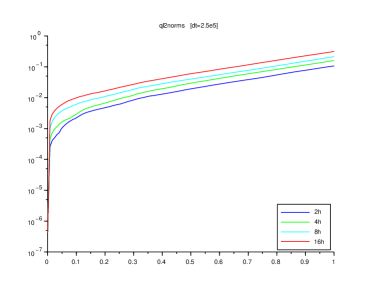
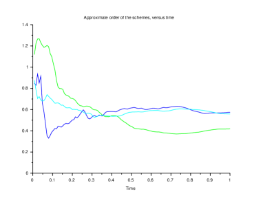
Figure 1. Figure showing the error and order of convergence with the SE-A scheme

4.2. ABAPO

We consider now a splitting scheme, where the Ornstein-Uhlenbeck portion is integrated analytically. We use the terminology from the splitting-scheme framework of [10], where we split the NELD dynamics into three portions,

$$\begin{split}d\begin{bmatrix}\mathbf{q}\\ \mathbf{p}\end{bmatrix}&=\underbrace{\begin{bmatrix}\mathbf{p}\\ 0\end{bmatrix}\,dt}_{A}+\underbrace{\begin{bmatrix}0\\ -\textsc{$\nabla E$}(\mathbf{q})\end{bmatrix}\,dt}_{B}+\underbrace{\begin{bmatrix}0\\ A\mathbf{p}\end{bmatrix}\,dt}_{P}+\underbrace{\begin{bmatrix}0\\ -\gamma(\mathbf{p}-A\mathbf{q})\end{bmatrix}\,dt+\begin{bmatrix}0\\ \sigma\,dW\end{bmatrix}}_{O}\end{split}$$ (11)

each of these split portions can be analytically integrated, $A,$ $B,$ and $P$ trivially so, while the exact solution of the $O$ part is

$$\begin{split}\mathbf{p}(t)=\exp(-\gamma\Delta t)\mathbf{p}(t_{0})+(1-\exp(-\gamma\Delta t))A\mathbf{q}(t_{0})+\sqrt{\beta^{-1}(1-\exp(-2\gamma\Delta t)}\bm{\xi},\end{split}$$ (12)

where

$$\bm{\xi}=\left(\frac{\beta}{1-\exp(-2\gamma\Delta t}\right)^{1/2}\exp(-\gamma t)\int_{t_{0}}^{t}\sigma\exp(\gamma s)\,dW(s)\sim\mathcal{N}(0,1).$$

We choose an ABAPO splitting, which is used in [1], to arrive at the numerical integrator

$$\begin{split}\psi_{ABAPO}^{\Delta t}=\exp\left(\frac{\Delta t}{2}\mathcal{L}_{A}\right)\exp(\Delta t\mathcal{L}_{B})\exp\left(\frac{\Delta t}{2}\mathcal{L}_{A}\right)\exp(\Delta t\mathcal{L}_{O})\end{split}$$ (13)

where $\mathcal{L}_{f}$ is the corresponding operator for the vector field $f$. It may be noticed that the phase ABA is the standard Verlet method.

GenKr PBCs is applied at the beginning of the scheme and after each integration in the position, in order to keep the particle inside the box. The ABAPO algorithm is described as follows:

Algorithm 2 ABAPO

for $k\leftarrow 1\dots$ Nsteps do

     GenKR($\mathbf{q}^{k},\mathbf{p}^{k}$) $\triangleright$ Apply PBCs

     $\mathbf{p}^{k+\frac{1}{4}}$ $\leftarrow$ $\mathbf{p}^{k}+\frac{\Delta t}{2}\textsc{$\nabla E$}(\mathbf{q}^{k})$

     $\mathbf{q}^{k+1}$ $\leftarrow$ $\mathbf{q}^{k}+\frac{\Delta t}{2}\mathbf{p}^{k+\frac{1}{4}}$

     GenKR($\mathbf{p}^{k+\frac{1}{4}},\mathbf{q}^{k+1}$)

     $\mathbf{p}^{k+\frac{1}{2}}$ $\leftarrow$ $\mathbf{p}^{k+\frac{1}{4}}+\frac{\Delta t}{2}\textsc{$\nabla E$}(\mathbf{q}^{k+1})$

     $\tilde{\mathbf{p}^{k+\frac{1}{2}}}$ $\leftarrow$ $\exp(\Delta tA)\mathbf{p}^{k+\frac{1}{2}}$

     $\mathbf{p}^{k+1}$ $\leftarrow$ $\gamma\tilde{\mathbf{p}^{k+\frac{1}{2}}}+(1-\gamma)A\mathbf{q}^{k+1}+\sqrt{\beta^{-1}(1-\exp(-2\gamma\Delta t)}\bm{\xi}$

We observe a similar loss of order of convergence as in the SE-A case, as displayed in Figure 2. There doesn’t seem to be a single observed rate of convergence, though it is clear that it is lower than first order.

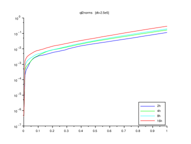
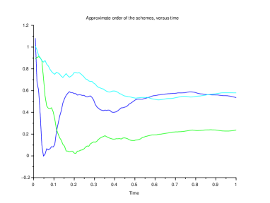
Figure 2. Figure showing the error and order of convergence with the ABAPO scheme

5. First Order NELD Algorithm

In this section, we will analyze four first order NELD schemes, two of which are corrected versions of Algorithms 1 and 2.

5.1. Euler-Maruyama

The Euler-Maruyama integrator for NELD differs from the SE-A algorithm above since we do not need to update the position before integrating the momentum, leading to only one application of the periodic boundary conditions. Thus we get the algorithm:

Algorithm 3 Euler-Maruyama

for $k\leftarrow 1\dots$ Nsteps do

    GenKR($\mathbf{q}^{k},\mathbf{p}^{k}$)

    $q_{tmp}$ $\leftarrow$ $\mathbf{p}^{k}+\mathbf{p}^{k}\Delta t$

    $\mathbf{p}^{k+1}$ $\leftarrow$ $\mathbf{p}^{k}+\textsc{F}(\mathbf{q}^{k},\mathbf{p}^{k})\Delta t+\sigma\sqrt{\Delta t}\bm{\eta}$

    $\mathbf{q}^{k+1}$ $\leftarrow$ $q_{tmp}$

Writing the update rule, and taking into account the application of PBCs, we have

$$\vspace{0.8 cm}\begin{split}\begin{bmatrix}\mathbf{q}^{k+1}\\ \mathbf{p}^{k+1}\end{bmatrix}&=\begin{bmatrix}\mathbf{q}^{k}-L\mathbf{n}\\ \mathbf{p}^{k}-AL\mathbf{n}\end{bmatrix}+\begin{bmatrix}\mathbf{p}^{k}-AL\mathbf{n}\\ \textsc{F}(\mathbf{p}^{k}-AL\mathbf{n},\mathbf{q}^{k}-L\mathbf{n})\end{bmatrix}\Delta t+\begin{bmatrix}0&0\\ 0&\sigma I\end{bmatrix}\sqrt{\Delta t}\bm{\eta}\\ &=\begin{bmatrix}\mathbf{q}^{k}-L\mathbf{n}\\ \mathbf{p}^{k}-AL\mathbf{n}\end{bmatrix}+\begin{bmatrix}\mathbf{p}^{k}-AL\mathbf{n}\\ \textsc{F}(\mathbf{q}^{k},\mathbf{p}^{k})-A^{2}L\mathbf{n}\end{bmatrix}\Delta t+\begin{bmatrix}0&0\\ 0&\sigma I\end{bmatrix}\sqrt{\Delta t}\bm{\eta}\\ \end{split}$$ (14)

Comparing with (9), we compute the leading orders of the local truncation error, finding $O(\Delta t^{3/2})$ stochastic terms and $O(\Delta t^{2})$ deterministic terms,

$$T_{2}=\begin{bmatrix}\textsc{F}(\mathbf{p},\mathbf{q})\\ (-\textsc{$\nabla^{2}E$}(\mathbf{q})+\gamma A)\mathbf{p}+(A-\gamma I)\textsc{F}(\mathbf{p},\mathbf{q})\end{bmatrix}\frac{\Delta t^{2}}{2}+\sigma\Delta t^{3/2}\begin{bmatrix}0&I\\ 0&(A-\gamma I)\\ \end{bmatrix}\left(\frac{1}{2}\bm{\eta}+\frac{1}{2\sqrt{3}}\bm{\zeta}\right)$$ (15)

Therefore, the scheme will converge to first order, which is confirmed numerically in Figure 3.

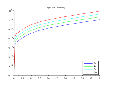
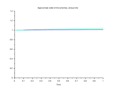
Figure 3. For the Euler-Maruyama method applied to NELD, we show the $\ell^{2}$ norm of the position differences (left) and estimated order of convergence graph as a function of time (right), which exhibits first-order convergence, consistent with the error analysis.

5.2. Symplectic Euler B (SE-B)

In Symplectic Euler B, the momentum is integrated first, then the position. The periodic boundary conditions need only be applied a single time during the inner loop, and we have the following pseudocode:

Algorithm 4 Symplectic Euler B

for $k\leftarrow 1\dots$ Nsteps do

    GenKR($p,q$)

    $\mathbf{p}^{k+1}$ $\leftarrow$ $\mathbf{p}^{k}$ + F($\mathbf{p}^{k+1},\mathbf{q}^{k}$) $dt+\sigma dW$

    $\mathbf{q}^{k+1}$ $\leftarrow$ $\mathbf{q}^{k}+\mathbf{p}^{k+1}\Delta t$

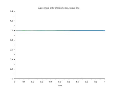
Figure 4. Order of convergence in position, using SE-B

The numerical scheme is implicit in $\mathbf{p},$ though it is linear in $\mathbf{p}^{k+1},$ and a perturbation of the identity, so that we can solve for $\mathbf{p}^{k+1}$ and expand in powers of $\Delta t,$ getting

$$\begin{split}\begin{bmatrix}\mathbf{q}^{k+1}\\ \mathbf{p}^{k+1}\end{bmatrix}&=\begin{bmatrix}\mathbf{q}^{k}-L\mathbf{n}\\ \mathbf{p}^{k}-AL\mathbf{n}\end{bmatrix}+\begin{bmatrix}\mathbf{p}^{k}-AL\mathbf{n}+(\textsc{F}(\mathbf{p}^{k+1},\mathbf{q}^{k}-L\mathbf{n}))\Delta t\\ \textsc{F}(\mathbf{p}^{k+1},\mathbf{q}^{k}-L\mathbf{n})\end{bmatrix}\Delta t+\sigma\begin{bmatrix}0&0\\ 0&I\end{bmatrix}dW\\ &=(I+(\gamma I-A)\Delta t)^{-1}\left(\begin{bmatrix}(I+(\gamma I-A)\Delta t)(\mathbf{q}^{k}-L\mathbf{n})\\ \mathbf{p}^{k}-AL\mathbf{n}\end{bmatrix}\right.\\ &\qquad+\begin{bmatrix}\mathbf{p}^{k}-AL\mathbf{n}+(-\nabla E(\mathbf{q}^{k})+\gamma A(\mathbf{q}^{k}-L\mathbf{n}))\Delta t\\ (-\nabla E(\mathbf{q}^{k})+\gamma A(\mathbf{q}^{k}-L\mathbf{n}))\end{bmatrix}\Delta t+\sigma\begin{bmatrix}0&\Delta t\\ 0&I\end{bmatrix}\sqrt{\Delta t}\bm{\eta}\big{)}\\ &=\begin{bmatrix}\mathbf{q}^{k}-L\mathbf{n}\\ \mathbf{p}^{k}-AL\mathbf{n}\end{bmatrix}+\begin{bmatrix}\mathbf{p}^{k}-AL\mathbf{n}\\ \textsc{F}(\mathbf{p}^{k},\mathbf{q}^{k})-A^{2}L\mathbf{n}\end{bmatrix}\Delta t+\begin{bmatrix}\textsc{F}(\mathbf{p}^{k},\mathbf{q}^{k})-A^{2}L\mathbf{n}\\ (A-\gamma I)(\textsc{F}(\mathbf{p}^{k},\mathbf{q}^{k})-A^{2}L\mathbf{n})\end{bmatrix}\Delta t^{2}\\ &\quad+\sigma\begin{bmatrix}0&0\\ 0&I\end{bmatrix}\Delta t^{1/2}\bm{\eta}+\sigma\begin{bmatrix}0&I\\ 0&(A-\gamma I)\end{bmatrix}\Delta t^{3/2}\bm{\eta}+O(\Delta t^{5/2})\\ \end{split}$$

As in the case of the Euler-Maruyama scheme, we find that the local truncation error is $O(\Delta t^{3/2})$ in the stochastic terms and $O(\Delta t^{2})$ in the deterministic terms,

$$T_{3}=\begin{bmatrix}-\textsc{F}(\mathbf{p},\mathbf{q})\\ (-\textsc{$\nabla^{2}E$}(\mathbf{q})+\gamma A)\mathbf{p}-(A-\gamma I)\textsc{F}(\mathbf{p},\mathbf{q})\end{bmatrix}\frac{\Delta t^{2}}{2}+\sigma\Delta t^{3/2}\begin{bmatrix}0&I\\ 0&(A-\gamma I)\\ \end{bmatrix}\left(-\frac{1}{2}\bm{\eta}+\frac{1}{2\sqrt{3}}\bm{\zeta}\right)$$ (16)

The global truncation error converges to the first order. The numerical results illustrated in Figure 4 confirm the analytical result.

5.3. Symplectic Euler A Corrected (SE-AC) and ABAPO Corrected (ABAPO-C)

The difference between ABA-O/SE-AC and the corrected schemes ABAPO-C/SE-AC presented here resides in the fact that applying periodic boundary conditions is only done once during the scheme, while interparticle forces $-\textsc{$\nabla E$}(\mathbf{q})$ are computed using the periodic conditions (while particles may rest outside of the box). Thus we get algorithms 5 and 6 for SE-AC and ABAPO-C, respectively.

Algorithm 5 Symplectic Euler A Corrected (SE-AC)

for $k\leftarrow 1\dots$ Nsteps do

    GenKR($\mathbf{q}^{k},\mathbf{p}^{k}$)

    $\mathbf{q}^{k+1}$ $\leftarrow$ $\mathbf{q}^{k}+\mathbf{p}^{k}\Delta t$

    $\mathbf{p}^{k+1}$ $\leftarrow$ $\mathbf{p}^{k}+\textsc{${F}_{\rm{PBC}}$}($ $\mathbf{p}^{k},$ $\mathbf{q}^{k+1}$ $)\Delta t+\sigma\sqrt{\Delta t}\bm{\eta}$

Algorithm 6 ABAPO-C

for $k\leftarrow 1\dots$ Nsteps do

    GenKR($\mathbf{q}^{k},\mathbf{p}^{k}$) $\triangleright$ Apply PBCs at the beginning of each iteration

    $\mathbf{p}^{k+\frac{1}{4}}$ $\leftarrow$ $\mathbf{p}^{k}+\frac{\Delta t}{2}\textsc{$\nabla E$}(\mathbf{q}^{k})$

    $\mathbf{q}^{k+1}$ $\leftarrow$ $\mathbf{q}^{k}+\frac{\Delta t}{2}\mathbf{p}^{k+\frac{1}{4}}$

    $\mathbf{p}^{k+\frac{1}{2}}$ $\leftarrow$ $\mathbf{p}^{k+\frac{1}{4}}+\frac{\Delta t}{2}{\textsc{$\nabla E_{\rm{PBC}}$}(\mathbf{q}^{k+1})}$

    $\tilde{\mathbf{p}^{k+\frac{1}{2}}}$ $\leftarrow$ $\exp(\Delta tA)\mathbf{p}^{k+\frac{1}{2}}$

    $\mathbf{p}^{k+1}$ $\leftarrow$ $\gamma\tilde{\mathbf{p}^{k+\frac{1}{2}}}+(1-\gamma)A\mathbf{q}^{k+1}+\sigma dW$

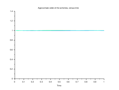
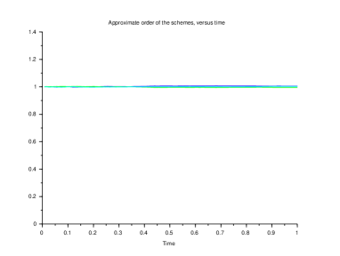
Figure 5. Order of convergence in position, using SE-AC (left) and ABAPO-C (right)

Expanding out SE-AC, we have a similar expression to SE-A (10), though there is only a single application of periodic boundary conditions, so we have

$$\begin{split}\begin{bmatrix}\mathbf{q}^{k+1}\\ \mathbf{p}^{k+1}\end{bmatrix}&=\begin{bmatrix}\mathbf{q}^{k}-L\mathbf{n}\\ \mathbf{p}^{k}-AL\mathbf{n}\end{bmatrix}+\begin{bmatrix}\mathbf{p}^{k}-AL\mathbf{n}\\ \textsc{F}(\mathbf{p}^{k}-AL\mathbf{n},\mathbf{q}^{k}-L\mathbf{n}+(\mathbf{p}^{k}-AL\mathbf{n})\Delta t)\end{bmatrix}\Delta t+\begin{bmatrix}0&0\\ 0&\sigma I\end{bmatrix}\bm{\eta}\\ &=\begin{bmatrix}\mathbf{q}^{k}-L\mathbf{n}\\ \mathbf{p}^{k}-AL\mathbf{n}\end{bmatrix}+\begin{bmatrix}\mathbf{p}^{k}-AL\mathbf{n}\\ \textsc{F}(\mathbf{q}^{k},\mathbf{p}^{k})-A^{2}L\mathbf{n}\end{bmatrix}\Delta t+\begin{bmatrix}0&0\\ 0&\sigma I\end{bmatrix}\sqrt{\Delta t}\bm{\eta}\\ &\quad+\begin{bmatrix}0\\ \gamma A(\mathbf{p}^{k}-AL\mathbf{n})-\textsc{$\nabla^{2}E$}(\mathbf{q}^{k})(\mathbf{p}^{k}-AL\mathbf{n})\end{bmatrix}\Delta t^{2}.\end{split}$$ (17)

Then the leading order terms in the local truncation error are $O(\Delta t^{3/2})$ in the stochastic terms and $O(\Delta t^{2})$ in the deterministic terms,

$$\begin{split}T_{4}&=\begin{bmatrix}\textsc{F}(\mathbf{p},\mathbf{q})+A^{2}L\mathbf{n}\\ (\textsc{$\nabla^{2}E$}(\mathbf{q})-\gamma A)\,\mathbf{p}+(A-\gamma I)\textsc{F}(\mathbf{p},\mathbf{q})\end{bmatrix}\frac{\Delta t^{2}}{2}+\sigma\Delta t^{3/2}\begin{bmatrix}0&I\\ 0&(A-\gamma I)\\ \end{bmatrix}\left(\frac{1}{2}\bm{\eta}+\frac{1}{2\sqrt{3}}\bm{\zeta}\right)\end{split}$$

Therefore, we expect to find first order convergence for the scheme, which is precisely what we observe in Figure 5. We similarly see the same improvement in convergence for the ABAPO-C scheme.

6. Second Order Integrator of the Langevin Equation A and B (SOILE-A & B)

We base our Second order NELD integrators on algorithms developed for equilibrium Langevin dynamics in [13]. Since we need to integrate the position first in both methods, we apply the ideas from the corrected algorithm where we wait to remap the particle positions until the end of the variable updates. The standard SOILE-A scheme is a generalization of the Langevin equation for velocity-Verlet algorithm while, SOILE-B is a quasi-symplectic scheme. The algorithms are described as follows:

Algorithm 7 Second Order Integrator of the Langevin Equation A (SOILE-A)

for $k\leftarrow 1\dots$ Nsteps do

     GenKR($\mathbf{q}^{k},\mathbf{p}^{k}$)

     $\mathbf{q}^{k+1}$ $\leftarrow$ $\mathbf{q}^{k}+\mathbf{p}^{k}\Delta t+\textsc{$F$}($ $\mathbf{p}^{k},$ $\mathbf{q}^{k}$ $)\frac{\Delta t^{2}}{2}+\Delta t^{3/2}(\frac{1}{2}\bm{\eta}^{k}+\frac{1}{2\sqrt{3}}\bm{\zeta}^{k})$

     $\mathbf{p}^{k+1}$ $\leftarrow$ $\mathbf{p}^{k}+(\textsc{${F}_{\rm{PBC}}$}($ $\mathbf{p}^{k},$ $\mathbf{q}^{k+1}$ $)+\textsc{$F$}($ $\mathbf{p}^{k},$ $\mathbf{q}^{k}$ $))\frac{\Delta t^{2}}{2}+\sigma dW-(\gamma I-A)(\textsc{$F$}($ $\mathbf{p}^{k},$ $\mathbf{q}^{k}$ $)\frac{\Delta t^{2}}{2}+\Delta t^{3/2}(\frac{1}{2}\bm{\eta}^{k}+\frac{1}{2\sqrt{3}}\bm{\zeta}^{k}))$

Algorithm 8 Second Order Integrator of the Langevin Equation B (SOILE-B)

for $k\leftarrow 1\dots$ Nsteps do

     GenKR($\mathbf{q}^{k},\mathbf{p}^{k}$)

     $\mathbf{p}^{k+1/2}$ $\leftarrow$ $\mathbf{p}^{k}+\frac{1}{2}\textsc{$F$}($ $\mathbf{p}^{k},$ $\mathbf{q}^{k}$ $)\Delta t-\frac{1}{4}(\gamma I-A)\big{[}\textsc{$F$}($ $\mathbf{p}^{k},$ $\mathbf{q}^{k}$ $)\frac{1}{2}\Delta t^{2}+\sigma\Delta t^{\frac{3}{2}}(\frac{1}{2}\bm{\eta}+\frac{1}{\sqrt{3}}\bm{\zeta})\big{]}$

     $\mathbf{q}^{k+1}$ $\leftarrow$ $\mathbf{q}^{k}+\mathbf{p}^{k+1/2}\Delta t+\sigma\Delta t^{\frac{3}{2}}\frac{1}{\sqrt{3}}\bm{\zeta}$

     $\mathbf{p}^{k+1}$ $\leftarrow$ $\mathbf{p}^{k+1/2}+\frac{1}{2}\textsc{$\tilde{F}_{\rm{PBC}}$}($ $\mathbf{p}^{k+1/2},$ $\mathbf{q}^{k+1}$ $)\Delta t+\frac{1}{2}\sigma\sqrt{\Delta t}\bm{\eta}-\frac{1}{4}(\gamma I-A)\big{[}\textsc{$\tilde{F}_{\rm{PBC}}$}($ $\mathbf{p}^{k+1/2},$ $\mathbf{q}^{k+1}$ $)\frac{1}{2}\Delta t^{2}+\sigma\Delta t^{\frac{3}{2}}(\frac{1}{2}\bm{\eta}+\frac{1}{\sqrt{3}}\bm{\zeta})\big{]}$

We write out the SOILE-A scheme, and expand out to second order, giving

$$\begin{split}\tilde{\begin{bmatrix}\mathbf{q}^{k+1}\\ \mathbf{p}^{k+1}\end{bmatrix}}&=\begin{bmatrix}\mathbf{q}^{k}-L\mathbf{n}\\ \mathbf{p}^{k}-AL\mathbf{n}\end{bmatrix}+\begin{bmatrix}\mathbf{p}^{k}-AL\mathbf{n}\\ \frac{1}{2}(-\textsc{$\nabla E$}(\mathbf{q}^{k+1})-\textsc{$\nabla E$}(\mathbf{q}^{k})+\gamma A(\mathbf{q}^{k+1}+\mathbf{q}^{k}))-(\gamma I-A)(\mathbf{p}^{k}-AL\mathbf{n})\end{bmatrix}\Delta t\\ &\quad+\begin{bmatrix}0&0\\ 0&\sigma I\end{bmatrix}\sqrt{\Delta}\bm{\eta}+\begin{bmatrix}\textsc{F}(\mathbf{q}^{k},\mathbf{p}^{k})-A^{2}L\mathbf{n}\\ 0\end{bmatrix}\frac{\Delta t^{2}}{2}+\begin{bmatrix}0&\sigma I\\ 0&\sigma(A-\gamma I)\\ \end{bmatrix}\Delta t^{3/2}(\frac{1}{2}\bm{\zeta}^{k}+\frac{1}{2\sqrt{3}}\bm{\eta}^{k})\\ &=\begin{bmatrix}\mathbf{q}^{k}-L\mathbf{n}\\ \mathbf{p}^{k}-AL\mathbf{n}\end{bmatrix}+\begin{bmatrix}\mathbf{p}^{k}-AL\mathbf{n}\\ \textsc{F}(\mathbf{q}^{k},\mathbf{p}^{k})-A^{2}L\mathbf{n}\end{bmatrix}\Delta t+\begin{bmatrix}0&0\\ 0&\sigma I\end{bmatrix}\sqrt{\Delta}\bm{\eta}\\ &\quad+\begin{bmatrix}\textsc{F}(\mathbf{q}^{k},\mathbf{p}^{k})-A^{2}L\mathbf{n}\\ -(\textsc{$\nabla^{2}E$}(\mathbf{q}^{k})+\gamma A)(\mathbf{p}^{k}-AL\mathbf{n})+(A-\gamma I)(\textsc{F}(\mathbf{q}^{k},\mathbf{p}^{k})-A^{2}L\mathbf{n})\end{bmatrix}\frac{\Delta t^{2}}{2}\\ &\quad+\begin{bmatrix}0&\sigma I\\ 0&\sigma(A-\gamma I)\\ \end{bmatrix}\Delta t^{3/2}\left(\frac{1}{2}\bm{\zeta}^{k}+\frac{1}{2\sqrt{3}}\bm{\eta}^{k}\right)+O(\Delta t^{3})\end{split}$$ (18)

These terms cancel with the exact expansion (9), with $O(\Delta t^{5/2})$ stochastic terms and $O(\Delta t^{3})$ deterministic terms, giving a globally second-order convergent scheme. We plot the order of convergence for both schemes in Figure 6, where we observe

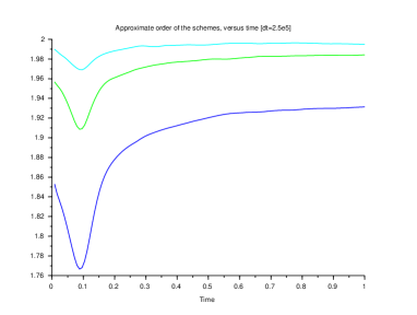
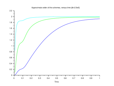
Figure 6. Estimated error of convergence for the SOILE-A (left) and SOILE-B (right) schemes. Both shown to be second order based on truncation error analysis, and the observed errors order is approximately second order. Note the different axes.

Moreover, we observe that the graphs of convergence 6 satisfy the second order scheme as predicted the truncation error. Note that both exhibit lower initial convergence, leveling off close to second order.

7. Conclusion

We have derived several numerical integrators for nonequilibrium Langevin dynamics and have shown that care must be taken in applying the periodic boundary conditions, or there can be a breakdown in the order of convergence. Provided that the pbcs are not applied in the middle of an update step, we have demonstrated several prototypical schems of order one and two applied to NELD. For these orders, deforming the domain is performed after all other updates, and we still acheive the desired accuracy.

Several extensions are possible. First, deriving conditions for general higher-order schemes that appropriately incorporate the deforming simulation box and nonequilibrium PBCs, for example, for general stochastic Runge-Kutta schemes or variational schemes will be of interest. Also, of large interest in molecular dynamics is the convergence to the invariant measure as in [1, 10]. This is challenging in the present case, since unlike Langevin dynamics, there is not generally an analytic expression for the invariant measure of the original dynamics (1).

8. Acknowledgements

MD was supported by the DARPA EQUiPS program.

References

- [1] Kevin Burrage and Grant Lythe. Accurate stationary densities with partitioned numerical methods for stochastic differential equations. SIAM Journal on Numerical Analysis, 47(3):1601–1618, 2009.
- [2] Matthew Dobson. Periodic boundary conditions for long-time nonequilibrium molecular dynamics simulations of incompressible flows. The Journal of Chemical Physics, 141(18):184103, 2014.
- [3] Matthew Dobson, Frédéric Legoll, Tony Lelièvre, and Gabriel Stoltz. Derivation of langevin dynamics in a nonzero background flow field. ESAIM: M2AN, 47(6):1583–1626, 2013.
- [4] Denis J. Evans and Gary P. Morriss. Statistical mechanics of nonequilibrium liquids. ANU E Press, Canberra, 2007.
- [5] Desmond J. Higham. An algorithmic introduction to numerical simulation of stochastic differential equations. SIAM Review, 43(3):525–546, 2001.
- [6] Thomas A. Hunt. Periodic boundary conditions for the simulation of uniaxial extensional flow of arbitrary duration. Molecular Simulation, 42(5):347–352, 2016.
- [7] Peter E. Kloeden and Eckhard Platen. Numerical Solution of Stochastic Differential Equations. Springer-Verlag Berlin Heidelberg, 1992.
- [8] A.M. Kraynik and D.A. Reinelt. Extensional motions of spatially periodic lattices. Int. J. Multiphase Flow, 18(6):1045 – 1059, 1992.
- [9] A W Lees and S F Edwards. The computer study of transport processes under extreme conditions. J. Phys. C Solid State, 5(15):1921, 1972.
- [10] Benedict Leimkuhler and Charles Matthews. Rational construction of stochastic numerical methods for molecular sampling. Applied Mathematics Research eXpress, 2013(1):34–56, 2013.
- [11] M.G. McPhie, P.J. Daivis, I.K. Snook, J. Ennis, and D.J. Evans. Generalized Langevin equation for nonequilibrium systems. Physica A, 299(3-4):412–426, 2001.
- [12] Ian Snook. The Langevin and Generalised Langevin Approach to the Dynamics of Atomic, Polymeric and Colloidal Systems. Elsevier, Amsterdam, 2007.
- [13] Eric Vanden-Eijnden and Giovanni Ciccotti. Second-order integrators for langevin equations with holonomic constraints. Chemical Physics Letters, 429(1-3):310–316, 9 2006.