New inclination changing eclipsing binaries
in the Magellanic Clouds

Abstract

Context. Multiple stellar systems are unique laboratories for astrophysics. Analysis of their orbital dynamics, if well characterized from their observations, may reveal invaluable information about the physical properties of the participating stars. Unfortunately, there are only a few known and well described multiple systems, this is even more so for systems located outside the Milky Way galaxy. A particularly interesting situation occurs when the inner binary in a compact triple system is eclipsing. This is because the stellar interaction, typically resulting in precession of orbital planes, may be observable as a variation of depth of the eclipses on a long timescale.

Aims. We aim to present a novel method to determine compact triples using publicly available photometric data from large surveys. Here we apply it to eclipsing binaries (EBs) in Magellanic Clouds from OGLE III database. Our tool consists of identifying the cases where the orbital plane of EB evolves in accord with expectations from the interaction with a third star.

Methods. We analyzed light curves (LCs) of 26121 LMC and 6138 SMC EBs with the goal to identify those for which the orbital inclination varies in time. Archival LCs of the selected systems, when complemented by our own observations with Danish 1.54-m telescope, were thoroughly analyzed using the PHOEBE program. This provided physical parameters of components of each system. Time dependence of the EB’s inclination was described using the theory of orbital-plane precession. By observing the parameter-dependence of the precession rate, we were able to constrain the third companion mass and its orbital period around EB.

Results. We identified 58 candidates of new compact triples in Magellanic Clouds. This is the largest published sample of such systems so far. Eight of them were analyzed thoroughly and physical parameters of inner binary were determined together with an estimation of basic characteristics of the third star. Prior to our work, only one such system was well characterized outside the Milky Way galaxy. Therefore, we increased this sample in a significant way. These data may provide important clues about stellar formation mechanisms for objects with different metalicity than found in our galactic neighborhood.

1 Introduction

It is well known that substantial part of all types of star in the solar neighborhood form binary or multiple stellar systems (e.g., Abt, 1983; Guinan & Engle, 2006). These systems include stars of all spectral types and all stages of their evolution. Proper description of their dynamical characteristics may result in determination of their physical parameters, and thus provide clues to their formation paths (e.g., Goodwin & Kroupa, 2005).

Despite the huge effort of astrophysicists in the field of stellar multiplicity in recent years, some mysteries about multiple systems still remain. For instance, recent results of thorough analysis of data from the Kepler mission have shown that there is a significant drop in population of triple systems with the period of a third component $P_{2}<200$ days (Borkovits et al., 2016). That is in accord with earlier results of Tokovinin (2014) who pointed out a similar drop of systems with the $P_{2}<1000$ days. The lull of systems at these intermediate $P_{2}$ values appears to be real and subject to severe selection effects. The theoretical explanation, however, still remains unknown.

Another uncertainty persists in the problem of dynamical stability. Mardling & Aarseth (2001) derived a theoretical limit on the stability of coplanar hierarchical triple systems as

$$P_{2}\gtrsim 4.7\biggl{(}\frac{m_{0}+m_{1}+m_{2}}{m_{0}+m_{1}}\biggr{)}^{1/10}\frac{(1+e_{2})^{3/5}}{(1-e_{2})^{S}}P_{1},$$ (1)

where $m_{0}$ and $m_{1}$ are masses of inner binary, $m_{2}$ is a mass of the third body, $e_{2}$ is an eccentricity of the outer orbit, and the parameter $s=1.8$. We follow the same notation hereafter. Sterzik & Tokovinin (2002) later improved this limit according to numerical simulations and showed that exponent $s$ in relation (1) has a different value, $s=1.35,$ to the best conformity between model and simulated data. However, it turned out later that there are only a few systems close to this limit and that the vast majority of observed triple systems fulfill an even stricter empirical criterion with the value of the exponent $s=3.0$ (Tokovinin, 2004, 2007). The lack of observed systems with high $e_{2}$ might be caused by unmodeled dynamical effects (Tokovinin, 2004) but generally the empirical stability criterion is still not satisfactorily explained. Nevertheless, recent analysis of 222 compact triples located in the original Kepler field of view performed by Borkovits et al. (2016) showed that the previously derived empirical criterion may rather be a result of some observational effects and all observed triples fulfils the theoretical criterion by Sterzik & Tokovinin (2002) (see Fig. 1). We point out that relation (1) is very useful for an estimation of maximal $e_{2}$ from the period ratio $P_{2}/P_{1}$, even if one has no information about individual body mass, because the period ratio dependence on masses is rather weak.

In spite of the intense research, there are still only a few multiple systems with precisely determined orbits and physical parameters of all components, especially out of the Milky Way galaxy. Therefore, studying the known multiple systems, as well as a search for new ones (especially those systems, which are close to the stability limit) is crucial for obtaining sufficient statistics and comparison of theoretical simulations with observational data.

Special cases, when the inner pair of a multiple system is an eclipsing binary, are excellent laboratories for stellar evolution. Light curve analysis together with thorough study of radial velocities are able to reveal physical parameters (such as luminosities, masses, and radii) of components of the EB, as well as its orbit (Southworth, 2012; Torres et al., 2010). One can also estimate some parameters of a third body which can manifest itself via various physical effects. These effects are listed below:

• eclipse time variations (ETVs) (Irwin, 1952; Mayer, 1990; Borkovits et al., 2016),

• presence of a third light in the LC solution or a third spectrum in the overall spectrum,

• visual resolution of the third body and its orbit,

• variation of $\gamma$-velocity of the binary,

• additional eclipses in a few rare cases (Carter et al., 2011; Borkovits et al., 2015; Alonso et al., 2015),

• variation of LC amplitude as a result of orbital plane precession (Söderhjelm, 1975b; Borkovits et al., 2016, 2011; Breiter & Vokrouhlický, 2015).

In the most favorable cases (e.g., high $L_{3}/(L_{1}+L_{2})$ ratio or almost coplanar orbits of EB and the third component) a combination effect can occur, which makes the estimation of the third body parameters more accurate. All these effects, except for the last one, are widely used for detection of new multiple systems. Effects of orbital precession led to discovery of a new triple only in relatively few cases mentioned in Sect. 3. Timescale of the orbital precession $P_{\mathrm{nodal}}\sim P_{2}^{2}/P_{1}$ is usually very long compared to the time span of the most extended observations that are available (about 100 years). Consequently, only those triples with sufficiently short periods of the outer orbits can be detected in available data sets. Because of this, there are still relatively few known systems showing orbital precession, despite the fact that all binaries with $P_{1}\lesssim 1$ day probably have a third companion which caused shrinkage of an initially wide orbit via combination of Kozai cycles with tidal friction (Kozai, 1962; Kiseleva et al., 1998; Eggleton & Kiseleva-Eggleton, 2001; Fabrycky & Tremaine, 2007) and orbital precession occurs in all cases when orbits are non-coplanar. An important step forward has been made recently by Rappaport et al. (2013) and Borkovits et al. (2016), who found $42$ new compact triples showing orbital precession in the original field of view of the Kepler satellite. Unfortunately there are far fewer such systems outside the Milky Way galaxy (see Sect. 3).

Only the compact triple systems with low ratio $P_{2}/P_{1}$ and short period $P_{2}$ can be discovered by analysis of amplitude variation of LC with typical timespan of several dozens of years. Interestingly, those systems fall exactly into the area of unclear lack of triples in Fig. 1, which makes this method very suitable for detection these systems and extending of their poor statistics. In this work, we aim to develop suitable methods for detecting those systems and their thorough analysis.

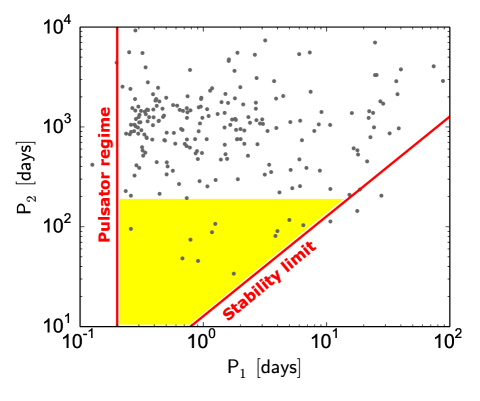
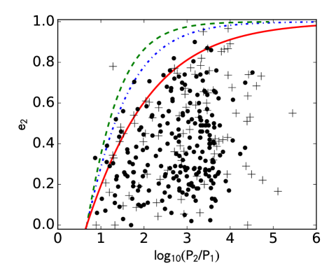
Figure 1: Left: Orbital period of the third companion $P_{2}$ versus orbital period of the inner binary $P_{1}$ for 222 triple systems within the original Kepler field (Borkovits et al., 2016). Area with the lack of triples is highlighted with yellow. The stability limit is calculated for the parameter $s=1.8$ in Eq. (1), with the assumption that $m_{0}=m_{1}=m_{2}=1$, for the mean value of orbital eccentricity of the outer orbit $\langle e_{2}\rangle\simeq 0.35$. Right: The eccentricity of the outer orbit as a function of the orbital period ratio. Dash-dot line is stability criterion according to Mardling & Aarseth (2001), dashed line (Sterzik & Tokovinin, 2002) and red solid line is empirical criterion according to observations of Tokovinin (2007). Eighty-eight triples from Multiple Star Catalog are plotted with black crosses (Tokovinin, 1997) and 222 triples in the original Kepler field are plotted with black dots (Borkovits et al., 2016).

2 Orbital-plane precession

While the orbital-plane precession results in variation of inclination of both orbits, only changes of inclination of the eclipsing binary are observable as changes of LC amplitude. Time dependence of observed inclination of the inner binary $i_{0}$ is given by the orbital geometry (Söderhjelm, 1975b)

$$\cos i_{0} =\cos I\cos i_{1}\pm\sin I\sin i_{1}\cos{\dot{\Omega}}(t-t_{0}),$$ (2)

$$\dot{\Omega} =\frac{2\pi}{P_{\mathrm{nodal}}},$$

where $I$ is an angle between system invariant plane and a plane tangent to the celestial sphere, $i_{1}$ is an angle between the invariant plane and the orbit of the EB, $t_{0}$ is a moment when the nodal line passes the plane tangent to the celestial sphere, $\dot{\Omega}$ is an angular velocity of the nodal line precession and $P_{\mathrm{nodal}}$ is a period of the nodal line precession. We recall that the invariant plane of the system is normal to its total and conserved orbital angular momentum. It is clearly seen that the observed inclination oscillates in the interval $i_{0}\in(I-i_{1},I+i_{1})$. Measuring time dependence of $i_{0}(t)$, we can use Eq. (2) to determine remaining parameters, which are deemed constant. These include $i_{1}$, $I$, ${\dot{\Omega}}$ and $t_{0}$. In what follows, we are mainly interested in solution of $i_{1}$ and ${\dot{\Omega}}$. Obviously, because of their non-linear appearance in (2), there are potentially severe correlations in their solution. We note also that Eq. (2) is invariant to the transformation $i_{1}\rightarrow\pi-i_{1}$ a $I\rightarrow\pi-I$ and the orbital solution is ambiguous.

In case that eccentricity of the orbit of the inner pair is $e_{1}\simeq 0$, which is fulfilled for a vast majority of short period binaries due to circularization, the precession rate of the nodal line in the invariant system may be derived analytically with a sufficient accuracy for most of the triple systems. We have

$$\dot{\Omega} \simeq\frac{2\pi}{P_{1}}\frac{3}{4\eta_{2}^{3}}\frac{m_{2}}{M_{2}}\biggl{(}\frac{P_{1}}{P_{2}}\biggr{)}^{2}\cos j\sqrt{1-\gamma^{2}+2\gamma\cos j},$$

$$\gamma =\frac{1}{\eta_{2}}\frac{l_{1}}{l_{2}}=\frac{1}{\eta_{2}}\frac{m_{0}m_{1}M_{2}P_{2}a_{1}^{2}}{m_{2}M_{1}^{2}P_{1}a_{2}^{2}},\;\eta_{2}=\sqrt{1-e_{2}^{2}},$$ (3)

$$M_{1} =m_{0}+m_{1},\;M_{2}=m_{0}+m_{1}+m_{2},\;j=i_{1}+i_{2},$$

where $i_{2}$ is an angle between the invariant plane and the orbital plane of the third body, $a_{k}$ is the semimajor axis and $l_{k}$ is the orbital angular momentum of the respective orbits (Breiter & Vokrouhlický, 2015). In these quantities, the indices $k=1$ and $k=2$ represent the inner and outer orbit, respectively. Angular velocity of the nodal line precession $\dot{\Omega}$ remains constant so long as the conditions $e_{2}=\mathrm{const.}$ and $j=\mathrm{const.}$ are fulfilled.

Modeling the variation of an EB inclination allows us to estimate the mass of the third body in the following way. Because $\sin i_{2}=\gamma\sin i_{1}$, the mutual inclination of both orbits $j=i_{1}+i_{2}$ can be rewritten as

$$j=i_{1}+\arcsin(\gamma\sin i_{1}).$$ (4)

Eliminating $a_{1}$ and $a_{2}$ from Eq. (2), we obtain for $\gamma$ the useful relation

$$\gamma=\frac{1}{\eta_{2}}\frac{m_{0}m_{1}}{M_{1}m_{2}}\biggl{(}\frac{P_{1}M_{2}}{P_{2}M_{1}}\biggr{)}^{1/3}.$$ (5)

The light curve solution together with spectra of components of the binary gives us the masses of the inner binary components $m_{0}$ and $m_{1}$. Therefore, $\gamma$ is only a function of $m_{2}$, $P_{2}$, and $e_{2}$, and thus ${\dot{\Omega}}={\dot{\Omega}}(i_{1},m_{2},P_{2},e_{2})$. The equation (2), applied to the observed dependence $i_{0}(t)$, gives a correlated least-squares fit of parameters $i_{1}$ and ${\dot{\Omega}}$. The size and shape of the area with possible solutions in the $(i_{1},{\dot{\Omega}})$ parameter space depend on the data time span and also on the period $P_{\mathrm{nodal}}$. In accordance with the functional dependence of ${\dot{\Omega}}$, each solution can be transformed to the $(m_{2},P_{2})$ parameter space, which leads to restrictions on the third body mass and its orbital period. Influence of unknown eccentricity $e_{2}$ on an estimation of $m_{2}$ and $P_{2}$ is rather small, because $\sqrt{1-e_{2}^{2}}\simeq 1$ even for $e_{2}$ values as large as $0.2-0.3$. In addition, maximal $e_{2}$ can be estimated according to the stability restrictions (see the right panel of Fig. 1).

A light curve solution leads to another restriction on the third body mass. A third body contributes with another light to the LC and it can be found during LC analysis in some cases. Then the third body mass can be estimated due to mass-luminosity relation. Even in cases when the third light is not detected, at least an upper limit on $m_{2}$ can be estimated.

Additional restriction on the third body mass can be obtained by analysis of ETVs. Orbital period $P_{2}$ is usually under the time resolution of long-term photometric surveys, because $P_{2}\sim\sqrt{P_{1}P_{\mathrm{nodal}}}$. Therefore, ETVs with period $P_{2}$ cannot usually be detected. Nevertheless, dispersion in eclipse timing residual diagram at least limits the maximal amplitude of ETVs. ETVs include classical Røemer’s delay (so called light-time effect (LTE)), caused by finite travel time of light (Irwin, 1952; Mayer, 1990), and so called dynamical delay, which means a physical variation of $P_{1}$ as a result of the gravitational interaction of components of the inner binary with the third body (Rappaport et al., 2013; Borkovits et al., 2003, 2011, 2015). Rappaport et al. (2013) showed that while Røemer’s delay is dominant for systems with a long period of the third component and a short period of the inner binary, dynamical delay is dominant for compact systems with a short period of the third component.

In this work, we deal with systems with $P_{1}$ of the order of days. Therefore, for period of a third body $P_{2}<200$ days (see Fig. 7 in Rappaport et al., 2013), dynamical delay dominates and the amplitude of ETVs is given by relation (Borkovits et al., 2003)

$$A_{\mathrm{phys}}=\frac{3}{8\pi}\frac{m_{2}}{m_{0}+m_{1}+m_{2}}\frac{P_{1}^{2}}{P_{2}}(1-e_{2}^{2})^{-3/2},$$ (6)

which allowed us to consider a restriction on relation $m_{2}=f(P_{2})$ because $A_{\mathrm{phys}}$ is bound from the dispersion of eclipse timing residual diagram and masses of the inner binary components can be estimated from LC solution. Conversely, for $P_{2}>200$ days classical Røemer’s delay dominates and ETVs amplitude is given as

$$A_{\mathrm{LTE}}=\frac{m_{2}\sin i_{3}}{(m_{0}+m_{1}+m_{2})^{2/3}}\frac{P_{2}^{2/3}\sqrt{1-e_{2}^{2}\cos^{2}\omega_{2}}}{173.15},$$ (7)

where the third body inclination $i_{3}$ oscilates within $(I-i_{2},I+i_{2})$ and its maximal values are known from the time dependence of $i_{0}$ (Irwin, 1952; Mayer, 1990). We note that factor $173.15$ holds when $A_{\mathrm{LTE}}$ and $P_{2}$ are given in days and masses are in units of solar mass. Outer orbit eccentricity $e_{2}$ is supposed to be unknown. However, Tokovinin (2007) showed that compact triple systems with high eccentricity of outer orbit $e_{2}$ becomes unstable and there is a natural limit on $e_{2}$ for each ratio of period $P_{2}/P_{1}$ (right panel of Fig. 1). According to selection effects of our methods, we can expect period ratios of analyzed systems within the interval $P_{2}/P_{1}\in(5,100)$ and therefore $e_{2}\leq 0.6$ in case of all systems analyzed below (see fig. 3 in Tokovinin, 2006).

3 Summary of known systems showing orbital precession

Only 53 systems showing orbital precession have been discovered in the Milky Way galaxy so far. While 11 of them have been found by different observers within various fields of view in the sky (see Table 1), 42 systems have been identified within the original Kepler field (Borkovits et al., 2016). Away from the Milky Way galaxy, 17 more systems are located in the Large Magellanic Cloud (LMC) (Graczyk et al., 2011; Zasche & Wolf, 2013) and there is only one known system in the Small Magellanic Cloud (SMC) (Pawlak et al., 2013).

Despite thorough analysis of the Kepler systems in our Galaxy, only one system outside the Milky Way galaxy has been carefully studied – MACHO 82.8043.171 (Zasche & Wolf, 2013). Studying multiple systems in external galaxies and improving statistics of known systems could help to reveal inter-galactic differences in star formation, which can be affected by different metallicity or other parameters and processes (Davies et al., 2015).

Table 1: Known inclination changing EBs in the Milky Way galaxy (42 EBs within the Kepler FOV are not included).

Designation	$P_{1}$	$P_{2}$	$P_{\rm nodal}$	Ref.
	(days)		(years)
RW Per	$13.1989$	$68$ yr	…	1, 2, 3, 4
IU Aur	$1.81147$	$294.3$ days	335	5, 6, 7, 8,
				9, 10
AH Cep	$1.7747$	$9.6$ yr	…	11, 12, 13
AY Mus	$3.2055$	…	…	14, 15
SV Gem	$4.0061$	…	…	16, 17, 18
V669 Cyg	$1.5515$	…	…	19, 20
V685 Cen	$1.19096$	…	…	21
V907 Sco	$3.77628$	$99.3$ days	$68$	22
SS Lac	$14.4161$	$679$ days	$600$	23, 24, 25
QX Cas	$6.004709$	…	…	26
HS Hya	$1.568024$	$190$ days	$631$	27, 28

(1) Hall (1969); (2) Mayer (1984); (3) Schaefer & Fried (1991); (4) Olson et al. (1992); (5) Mayer (1971); (6) Mayer & Drechsel (1987); (7) Mayer (1987); (8) Mayer et al. (1991); (9) Drechsel et al. (1994); (10) Mason et al. (1998); (11) Mayer (1980); (12) Drechsel et al. (1989); (13) Kim et al. (2005); (14) Söderhjelm (1975a); (15) Söderhjelm (1974); (16) Guilbault et al. (2001); (17) Paschke (2006); (18) Paschke (2006); (19) Azimov & Zakirov (1991); (20) Lippky & Marx (1994); (21) Mayer et al. (2004); (22) Lacy et al. (1999); (23) Milone et al. (2000); (24) Torres & Stefanik (2000); (25) Torres (2001); (26) Guinan et al. (2012); (27) Zasche & Paschke (2012); (28) Torres et al. (1997).

Large databases of medium quality lightcurves of EBs in the LMC and SMC, from photometric surveys like OGLE (Udalski, 2003; Udalski et al., 1997, 2008, 2015a, 2015b; Szymanski, 2005) or MACHO (Bennett et al., 1993; Cook et al., 1995), allow us to develop new methods to find candidate triple systems in the Magellanic Clouds. The goal of our study is to identify new LMC and SMC compact multiple systems via detection of amplitude variations in archival LCs. These amplitude variations could be caused by an orbital precession due to the presence of a third body. Because of rather short timescale of photometric surveys (in the order of ten years) and typically long timescales of orbital precession it is possible to find only systems with short $P_{2}$ and small ratio $P_{2}/P_{1}$. However, those systems should be exactly in the area with lack of triples in the $P_{1}-P_{2}$ distribution (yellow area in the Fig.  1) near stability limit, which makes this simple method suitable for identifying new compact triples.

4 Methods

Light curves of eclipsing binaries observed by the OGLE III photometric survey have sufficient precision, low scattering and good homogeneity over the whole term of observation. This makes this database suitable for finding new compact multiple systems in the Magellanic Clouds. The OGLE III database contains LCs of $26\,121$ EBs in the LMC (Graczyk et al., 2011) and $6138$ EBs in the SMC (Pawlak et al., 2013) (mostly in Johnson I photometric band) which are available online (Szymanski, 2005).

EB light curve amplitude variation can be caused by several effects, for example, physical variations of luminosity of the EB components, stellar spots, changes of overlapping surfaces during eclipses as a result of apsidal motion, etc. Therefore, when the maximum luminosity of both components remains constant and the orbit is circular, the only possible explanation of amplitude changes is that the inclination angle varies. Both conditions can be easily checked from phased light curve (PLC).

In principle, there may be two basic methods for detection of LC amplitude variations:

• Method A – measurement of the eclipse depth of a PLC in different time intervals,

• Method B – measurement of the amplitude of a non-phased LC in different epochs.

A typical number of data points $N$ in an OGLE III light curve is within the interval $(400,600)$, from which only a small fraction is located near eclipses (in the case of the most frequent EB type – detached binaries). Because of that, the number of time intervals has to be small to get a reasonable fit of minima shapes. Therefore, we had no ambition to detect other but linear amplitude changes on the timescale of OGLE III observations ($\approx 8$ years), in the case of Method A.

4.1 Data preparation

Ephemerides and classification of each EB were taken from OGLE III catalog (Graczyk et al., 2011). Only those LCs that contain sufficient amount of data points ($>250$) were taken into account. Those LCs, where the primary minima depth were smaller than the standard deviation of magnitudes, were discarded. It should be mentioned that it obviously add an artificial selection effect to the analysis, because shallow minima may be caused by massive and luminous third companion. But this restriction is necessary to avoid false detection due to high scattering of some LCs.

For the purpose of removing outliers, each LC was fitted with a linear function $f(t)$ and all data points outside the intervals $(f(t)-3\sigma,f(t)+7\sigma)$ in the case of detached binaries, $(f(t)-3\sigma,f(t)+6\sigma)$ in the case of semidetached binaries and $(f(t)-3\sigma,f(t)+3\sigma)$ in the case of overcontact binaries, were removed. We note that $\sigma$, in this case, means a standard deviation computed from the whole LC. These asymmetrical intervals were chosen with respect to different characters of LCs of individual EB types so that the whole LC (except outliers) lies inside the interval.

4.2 Method A

As the first step of this method, the whole LC of a given EB is divided into several intervals which contain approximately $150$ data points. A number of intervals depends on the number of data points in the whole LC. As shown in the left panel of Fig. 2, a typical LC has been divided into three or four intervals.

In the next step, the LC in each interval is phased according to the catalog ephemerides, in order to obtain a dependence of magnitude in the Johnson $I$ band on the phase $I(\Phi)$. The core of this method is based on fitting of primary minimum on each phased interval of the LC with a proper phenomenological function, which is able to describe well the depth of an eclipse. There is a class of mathematical functions which generate similar dependencies such as shapes of real LCs around eclipse (Andronov, 2012a, b; Mikulášek et al., 2012; Mikulášek, 2015). For our purposes we used the following formula (taken from Andronov, 2012a)

$$I(\Phi)=I_{0}+A\left\{1-\left[\left(\Phi-\Phi_{0}\right)/d\right]^{2}\right\}^{C},$$ (8)

where $I_{0}$ is a vertical shift in magnitude, $A$ is the depth of the eclipse, $\Phi_{0}$ is a phase of the time of minimum, $d$ represents minima width and $C$ is a parameter determines a shape of the eclipse. An example of fitted minima on each interval of the whole LC is shown in the Fig. 3.

However, Eq. (8) describes well only a small part of the PLC around minimum and each PLC had to be properly reduced before fitting. As a reasonable compromise between robustness of the algorithm and its computing speed, preliminary fitting of the PLCs with Fourier series of the fifth, fourth, and second orders were performed in the case of detached, semidetached and overcontact binaries, respectively (see the right panel of Fig. 2). The minimum of the Fourier model corresponds to the minimum of given PLC and the first maxima of this model on both sides of an eclipse define the whole part of drop in brightness (see the right panel of Fig. 2).

Minima depths (the parameter $A$ from the Eq. (8)) were registered on each interval of the whole LC and finally, the linear model of its time dependence was computed. For each EB, the slope of the linear fit and $R^{2}$ parameter were tested and if some specific values were exceeded, the EB was marked as suspicious of the inclination change. Further details about setting these values are described in Sect. 4.4.

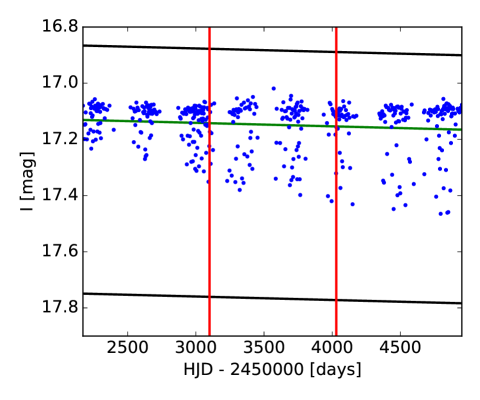
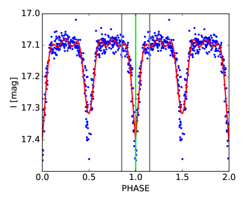
Figure 2: Demonstration of Method A. Left: Example LC of the system OGLE-LMC-ECL-01350 divided to three intervals. Green line represents linear fit, black lines show the limits for removal of the outliers ($-3\sigma$, $+7\sigma$). Right: Phase curve for the whole LC fitted with a Fourier series of the $5^{\mathrm{th}}$ order (red line). Green line marks detected primary minimum, gray lines represent detected region of the drop in brightness.

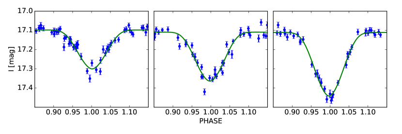
Figure 3: Demonstration of Method A. Fitting of primary eclipses of OGLE-LMC-ECL-01350 with function (8) on three intervals of LC, corresponding to the left panel of Fig. 2. The increase of the minima depth is apparent.

4.3 Method B

In the second method, the whole LC was split into eight fixed intervals with respect to the seasons of observation (see Fig. 4). In contrast with Method A, Method B is less demanding as far as the number of data points in a given interval is concerned, because it is not necessary to have a lot of points around the eclipse and that allows division of the LC to more intervals. After LC splitting, two data points corresponding to the lowest brightness were selected from each of the intervals of the LC and than all chosen data points were fitted with the linear model according to the $\sigma$-clipping method with a rejection of each point above the $2\sigma$ limit. As in the case of Method A, the detection criteria are the certain values of the slope of linear fit and the $R^{2}$ parameter. The setting of those values is described in Sect. 4.4.

The advantage of this simple method is that there is no need to know a precise orbital period of given EB and also there is no need to delimit a part of the LC with an eclipse. That makes this method faster than the Method A. On the other hand, what is actually fitted in this case, is not exactly the minimum depth, but only local LC amplitude, which makes this method more sensitive to outliers than slower fitting minima in each part of LC.

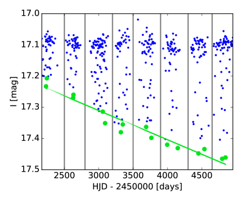
Figure 4: Demonstration of Method B. Example LC of the system OGLE-LMC-ECL-01350 splitted into 8 intervals according to observational seasons. The lowest two points inside each interval are plotted with green circles, the green line shows the linear fit.

4.4 Parameter thresholds

Specific values of slope and $R^{2}$ in the case of both methods served as thresholds for preliminary distinction whether changes of inclination occur in case of given EB or not. Setting of certain thresholds on these quantities is difficult because of the high variability of LC shape and their scattering that strongly depends on the brightness of a particular EB. However, the estimation of the threshold can be made in the parameter space defined by the 17 known systems in the OGLE III LMC database (Graczyk et al., 2011).

These systems, together with two others, which have been found independently by the second author of this paper, are shown in the parameter space of both methods in the Fig. 5. However, careful examination of the previously known systems from Graczyk et al. (2011) showed that in some cases the change of the amplitude of LC could rather be an artefact than a real feature. Furthermore, in some cases, amplitude variation is so fast that a significant part of LC is completely without eclipses. As described above, our ’linear’ methods are usually not able to detect such systems (e.g., OGLE-LMC-ECL-17212, 17972, see Fig.  5) and parameters thresholds were set irrespective of these systems.

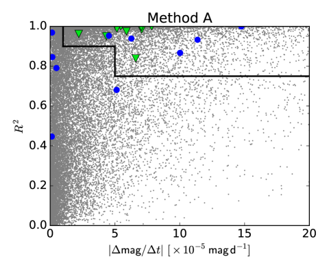
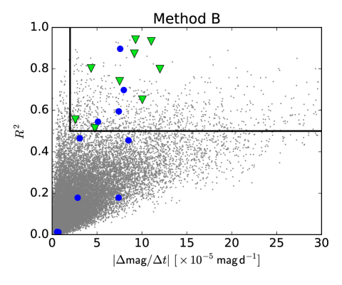
Figure 5: All eclipsing binaries from the OGLE III LMC database (gray dots) plotted in the (slope, $R^{2}$) parameter space of both methods. Nineteen previously known systems showing variations of the LC amplitude are marked with blue circles (artefacts or systems with rapid changes of amplitude) and green triangles (systems with approximately linear amplitude change on the timescale of observation). Our setting of thresholds is shown as a black line.

Systems with approximately linear time dependence of eclipse depth on the OGLE III observational time scale (see Fig. 5) served for setting the parameters thresholds. The area of interesting systems in the parameter space was chosen to exclude as many EBs as possible without any amplitude change. Finally, our empirical thresholds for the Method A were $|\Delta\mathrm{mag}/\Delta t|\geq 5\times 10^{-5}\;\mathrm{mag\,day^{-1}}$ and $R^{2}\geq 0.75$. However, some well covered LCs with very slow changing of amplitude could exist and for these systems the slope threshold is too strong. For this reason the restrictions were alleviated, and systems with $|\Delta\mathrm{mag}/\Delta t|\geq 1\times 10^{-5}\;\mathrm{mag\,day^{-1}}$ and $R^{2}\geq 0.90$ were marked as suspicious (see the Fig. 5). For Method B the following thresholds were set: $|\Delta\mathrm{mag}/\Delta t|\geq 2\times 10^{-5}\;\mathrm{mag\,day^{-1}}$ and $R^{2}\geq 0.50$.

In order to identify systems with shorter timescales of orbital precession ($P_{\mathrm{nodal}}\sim 10$ years) it was neccessary to modify our methods so that they could fit time dependence of LC amplitude by polynomials of higher orders. Method A cannot be modified in this way because it demands a relatively high number of data points around eclipses. But in Method B, LC is divided to eight intervals and the number of fitted data points is mostly 16, which allowed us to apply this modification.

Considering a scattering and coverage of LCs, polynomials up to the fourth order were used. Systems fulfilling the following criteria were marked as suspected of being of higher order amplitude variations:

• At least one higher-order polynomial fit (second, third, or fourth) was significantly better than a linear fit.

• At least one higher-order polynomial fit had to have AIC (Akaike, 1974), AICc (Sugiura, 1978) and BIC (Schwarz, 1978) information criteria value lower than a linear fit.

• $\chi^{2}$ of the higher-order polynomial fit was smaller than 50 to avoid systems with highly scattered data points around eclipses.

5 Results of detection of new systems with amplitude variation

Our methods described in Sect. 4 were applied to all light curves of eclipsing binaries from the OGLE III LMC+SMC. Thresholds set on the Method A and the linear regime of the Method B were exceeded in $8.1$ % and $3.1$ % of the LMC EBs, respectively. In the SMC it was in $3.9$ % and $2.8$ %. In the higher-order polynomial regime of Method B, $1.5$ % of LMC EBs and $1.4$ % of SMC EBs were marked as suspected of LC amplitude variations. All of the positive detections were subjects of thorough visual inspections and most of them were rejected as false positives.

False detections were mostly caused by too few data points around eclipses, which affects results of both methods. This is, for example, the case of OGLE-LMC-ECL-10172, which is a nice example of the system with rapid variation of LC amplitude during the term of OGLE III observations. However, the orbital period of the eclipsing binary is $P_{1}=1.993644$ d, which makes impossible to observe eclipses in some seasons from one observing site and an artificial change of the LC amplitude occurs.

Results of Method A strongly depend on a precision of the catalog value of a binary orbital period, and also on time stability of the light curve. In some cases, the mid-eclipse times of an EB vary in time due to apsidal motion or ETVs. That leads to ’blurriness’ of a PLC, and results obtained by Method A may have been irrelevant and had to be rejected.

In addition, some systems had to be rejected because of variations of maximal brightness (magnitude at quadratures), which may be caused by a motion of surface spots, physical variability of one or both components of a binary, or by a drift of zero points in the measuring equipment.

After visual inspection and combining results of both methods 51 and 21 candidates remained in the LMC and SMC samples, respectively. These systems are listed in Tables 2 and 3 together with cross-identifications with the OGLE II and MACHO surveys and their lightcurves are shown in appendices 8 and 12. Apart from the 13 previously known systems, there are 38 new systems in LMC, clearly showing amplitude variations while maximal brightness remains constant. From the 21 systems detected within the SMC, only one was previously known (Pawlak et al., 2013).

Table 2: Detected systems with change of LCs amplitudes in the LMC.

OGLE III LMC	OGLE II LMC	MACHO	Ref.
01350	…	…	1
02064	…	17.1985.175	this work
02269	…	45.2118.679	this work
02480	…	…	1
02641	…	…	this work
03163	…	17.2472.176	1
03183	…	17.2473.43	this work
03747	…	…	this work
04002	…	…	this work
06385	SC14_175132	…	1
06464	SC14_160905	1.3930.1050	this work
08377	…	…	this work
08628	…	…	this work
09770	SC10_255818	…	this work
10063	…	…	this work
10338	SC9_127779	79.5378.336	this work
10369	SC9_128347	…	this work
10413	SC9_127854	79.5378.26	this work
11068	…	…	this work
11658	SC8_205379	78.5859.237	this work
11168	…	49.5774.50	this work
13150	…	3.6485.107	this work
13399	…	…	this work
14394	SC5_169494	…	1
15256	…	…	this work
15520	SC4_227322	77.7433.183	this work
15993	SC4_391534	…	this work
16023	SC4_468053	77.7554.200	this work
16323	…	…	this work
16495	…	…	this work
16896	…	…	this work
17209	…	…	this work
17212	…	…	1
17359	…	82.8043.171	1, 2
17890	…	…	1
17972	…	…	1
18240	…	…	1
18686	…	…	1
19066	SC1_152384	…	this work
20389	…	…	this work
20742	…	…	this work
21083	…	…	this work
21928	…	…	1
22555	…	…	1
22686	…	33.9990.38	this work
22885	…	…	this work
22918	…	…	this work
23148	…	50.10240.867	this work
24123	…	…	this work
25108	…	…	this work
25373	…	…	this work

(1) Graczyk et al. (2011); (2) Zasche & Wolf (2013)

Table 3: Detected systems with change of LCs amplitudes in the SMC.

OGLE III SMC	OGLE II SMC	MACHO	Ref.
0648	…	…	this work
0718	…	208.15571.181	this work
0863	SC3_193792	…	this work
0917	SC4_14872	212.15677.1029	this work
1532	SC5_11681	…	this work
1649	SC5_123484	…	this work
1872	SC5_160326	212.15957.454	this work
1946	SC5_230499	…	this work
1989	SC5_311575	…	this work
2212	SC6_18013	…	this work
2436	SC6_94470	…	this work
3317	SC7_115374	211.16311.196	this work
3473	SC7_169045	…	this work
3613	SC8_46187	207.16431.1821	this work
3833	SC8_107524	207.16490.174	this work
4935	SC10_65845	206.16888.123	this work
4952	…	…	this work
5096	SC10_134445	…	1
5662	…	…	this work
5943	…	…	this work
6118	…	…	this work

(1) Pawlak et al. (2013)

6 Analysis of individual systems

Several detected systems showing LC amplitude variation were selected and analyzed thoroughly. The analysis was performed especially for systems with additional archival data (MACHO or OGLE II/IV) available.

For four selected systems, new Charge-coupled device (CCD) photometry was obtained at the La Silla Observatory in Chile, with 1.54-m Danish telescope in the Johnson $I$ photometric band to secure consistency with the OGLE data. For one system – OGLE-SMC-ECL-1532 – archival CCD frames, taken in the Johnson $R$ photometric band with the Danish telescope, were used. For aperture photometry we developed and used Python 2.7 scripts with usage of the photutils package and differential magnitudes were obtained. The individual data (HJD vs. $\Delta m$) are listed in Table 4.

Table 4: Photometric observations of individual systems.

LMC01350		LMC13150		LMC16023		LMC18240		LMC23148		SMC1532
JD	$\Delta m$	JD	$\Delta m$	JD	$\Delta m$	JD	$\Delta m$	JD	$\Delta m$	JD	$\Delta m$
6262.64078	-0.534	7376.54703	0.563	7323.57195	0.998	6263.55449	0.684	7318.55154	0.264	6211.79967	0.509
6262.64211	-0.538	7376.54982	0.545	7323.57893	1.009	6263.55583	0.690	7318.55294	0.270	6211.80180	0.516
6262.64345	-0.481	7376.56837	0.575	7323.58033	1.026	6263.55718	0.711	7318.55436	0.282	6211.80391	0.545
6262.64478	-0.495	7376.57117	0.558	7323.59018	1.037	6263.62203	0.622	7318.55575	0.296	6211.80602	0.506
6262.64612	-0.467	7376.58991	0.559	7323.62295	1.044	6263.62336	0.651	7318.56420	0.263	6211.80815	0.532
6262.64746	-0.468	7376.59133	0.546	7323.68933	1.073	6263.62469	0.641	7318.56559	0.280	6211.81027	0.498
6262.64879	-0.511	7376.59275	0.549	7323.69211	1.085	6263.62602	0.629	7318.56697	0.296	6211.81412	0.536
6262.65012	-0.492	7376.61125	0.557	7323.70622	1.070	6263.62736	0.645	7318.56837	0.266	6211.81624	0.493
6262.65146	-0.471	7376.61265	0.582	7323.72312	1.059	6263.62869	0.623	7318.56978	0.279	6211.81836	0.510
6262.65279	-0.484	7376.61405	0.574	7323.72450	1.033	6263.63002	0.640	7318.57811	0.289	6211.82045	0.529

Analysis of LCs of individual systems was performed in PHOEBE (Prša & Zwitter, 2005) program. Obtaining of spectra of the stars outside of the Milky Way galaxy is complicated and requires long exposure time even when using the largest telescopes. For this reason, a radial velocity curve is not available for any studied system and the mass ratio was fixed as $q=1$ in the first iteration of the LC modeling. When the photometric model was inconsistent with this assumption, it was recalculated with new $q$ value estimated from bolometric magnitudes of components. Synchronous rotation $F_{1}=F_{2}=1$ of both components was assumed and limb darkening coefficients were obtained from the square-root model which is more suitable for hot stars than the logarithmic model (Diaz-Cordoves & Gimenez, 1992). Bolometric albedos and gravity darkening were fixed as $A_{1,2}=g_{1,2}=1$ which is fulfilled for stars with $T>7200$ K whose subsurface layers are in radiative equilibrium. Without any specroscopic data for given stars, solar metallicity was assumed and fixed.

The basic model was computed on a subset with the lowest data scattering and the best coverage and on the other subsets inclinations $i_{0}$ and luminosities $L_{1,2}$ were fitted only. With the assumption that physical parameters of components remain constant, that led us to obtain a time dependence of binary inclination.

To improve the orbital period of the binary, primary and secondary minima were computed with the use of slightly modified AFP method (for the description of the original AFP method see Zasche et al., 2014) and eclipse timing residual diagram for each system was constructed. Modification of the original AFP method was neccessary due to the fact that LC amplitudes of our systems vary with time. Therefore, we had to fit not only a phase and magnitude shift of the model curve, but also its ’contraction’, which represents amplitude variation of the LC.

The final fixed parameter was primary temperature $T_{1}$ which had to be estimated from photometric indices because of a lack of another spectral information about given star in the LMC and SMC. However, correct estimation of the temperature is usually quite tricky. There are many photometric catalogs of the Magellanic Clouds with various color indices for a given star, which sometimes lead to different temperatures. In the case of the hot stars in our sample, relative differences in temperatures are up to $20\,\%$. Therefore, temperatures and masses of an individual component of an EB can be computed wrongly, which can also affect an estimated mass of the third body. But precision of estimation of the nodal period remains unaffected. For each system, all available color indices were collected and for the $T_{1}$ estimate the most probable value was selected. Each color index was also corrected from an effect of interstellar reddening, according to the relation $(B-V)_{0}=f((B-V),(U-B))$ (Johnson & Morgan, 1953), a map of interstellar reddening in the LMC (Haschke et al., 2011) and mean reddening in the direction toward the SMC (Massey et al., 1995).

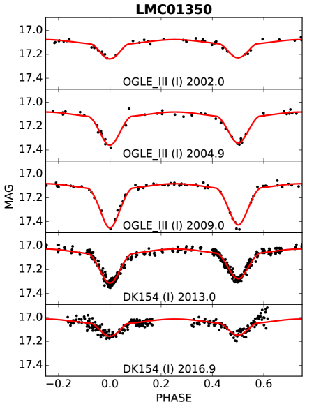
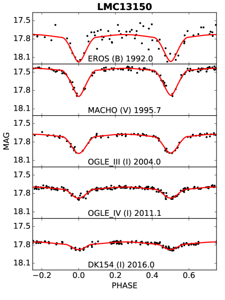
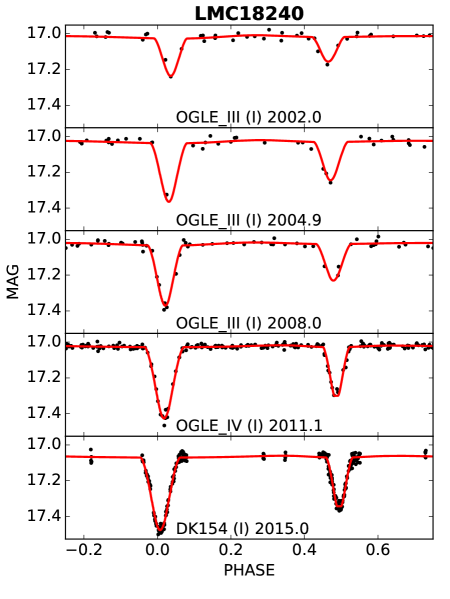
Figure 21: Light curves of selected eclipsing binaries. Only several modeled LCs for each system are shown. For each LC, survey designation, photometric band, and central time of given interval are listed.

Photometric solutions of LCs of individual systems in the LMC and SMC are in Tables 11 and 12, respectively. In these tables, the computed and fixed parameters are marked. Luminosities in $V$ and $R$ Johnson photometric bands were obtained from the MACHO data. MACHO photometry was not originally obtained in standard Johnson passbands but with $B_{\mathrm{MACHO}}$ and $R_{\mathrm{MACHO}}$ filters instead, and it had to be transformed before the PHOEBE modeling according to the calibration relations in (Bessell & Germany, 1999). Examples of LCs of each system, from which the time variations of inclination is apparent, are shown in Fig. 21.

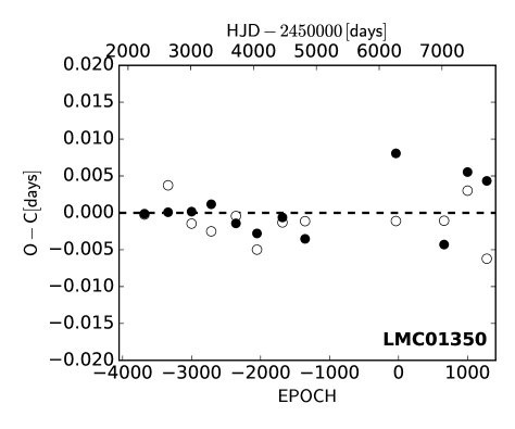
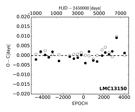
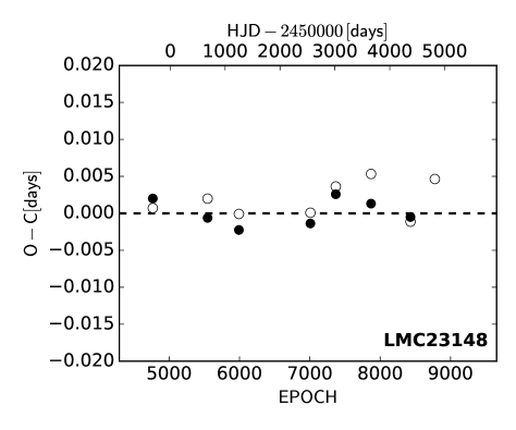
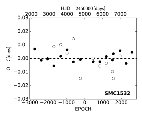
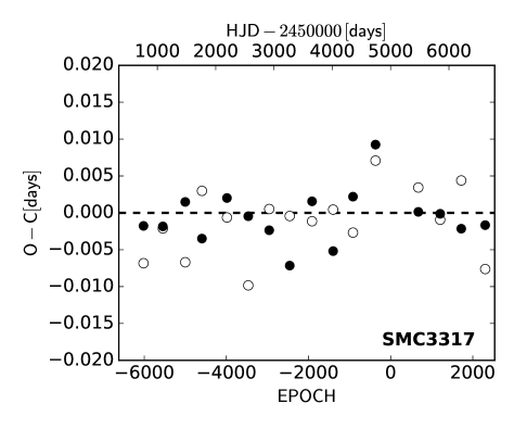
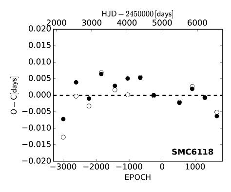
Figure 20: Eclipse timing residual (observed $-$ computed) diagrams for selected systems with respect to mean linear ephemerides listed in tables 13 and 14. Black and white points represent primary and secondary minima, respectively.

Precise linear ephemerides of the inner eclipsing binaries in the LMC and SMC are listed in Tables 13 and 14, respectively. In some cases, eclipse timing residual diagram of the EB is not linear and ETVs become apparent. For precise modeling of LCs of such systems several sets of linear ephemeris had to be calculated for each part of a given LC. In Tables 13 and 14, there are both the best ephemerides on whole time interval of observation and the set of ephemerides for each interval in cases when it was needed. Eclipse timing residual diagrams for every studied system is shown in Figs. 6 and 20.

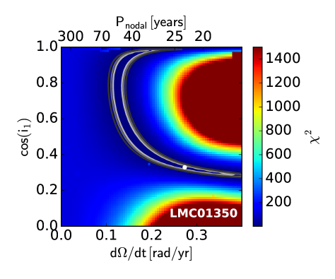
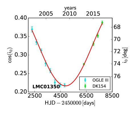
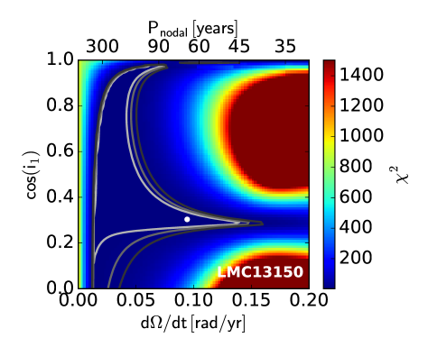
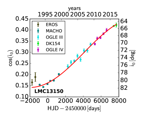
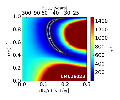
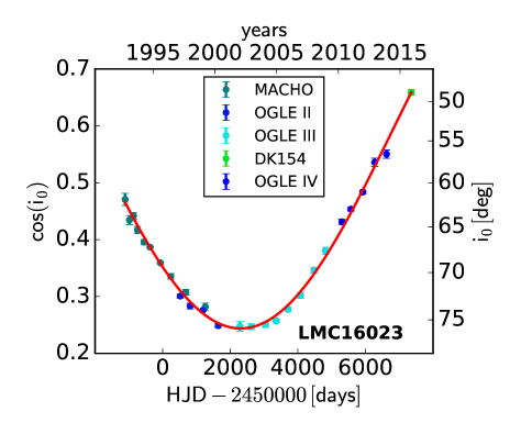
Figure 14: Left: Projections of $\chi^{2}$ of fitted dependence $\cos(i_{0})=f(t)$ to $\cos(i_{1})$ – $\dot{\Omega}$ plane. Confidence intervals $68.3\,\%$, $90.0\,\%$ and $99.0\,\%$ are indicated with gray lines. White points show the best solutions whose parameters are listed in Tables 5 and 6. Right: The best solution of dependence $\cos(i_{0})=f(t)$ according to relation (2).

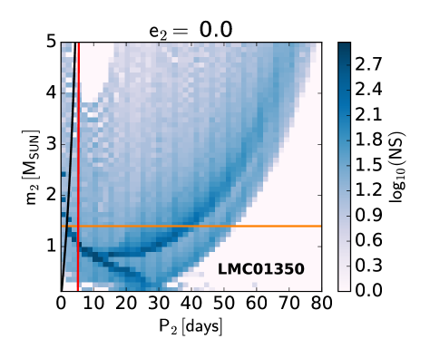
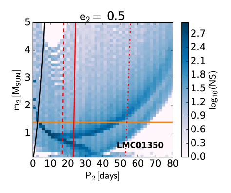
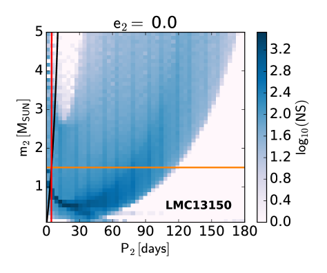
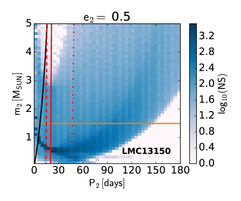
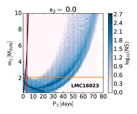
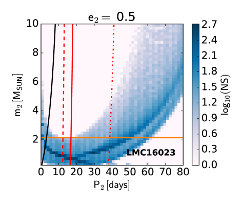
Figure 17: Possible masses and periods of third bodies. All solutions from $68.3\,\%$ area in the Fig. 14 for possible orientations $i_{1}\rightarrow\pi-i_{1}$ and $I\rightarrow\pi-I$ are shown. Logarithmic scale of a number of solutions (NS) is shownin blue. The orange line indicates the maximal third body mass according to the limit of a third light from the LC solution. (Continued on next page.)

Photometric solution of each LC subset of each system enables to derive the time dependence of inclination $i_{0}(t)$ of every EB. In order to obtain $P_{\mathrm{nodal}}$, physical parameters of a third body and mutual orientation of orbits, each dependence $\cos(i_{0})=f(t)$ was modeled with Eq. (2). The results are listed in Tables 5 and 6 together with $68\%$ confidence intervals. Confidence interval of each fitted parameter was estimated from projection of $\chi^{2}$ of the fit of $\cos(i_{0})=f(t)$ dependence. In Fig. 14, there is $\chi^{2}$ of the fit shown in $\cos(i_{1})$ - $\dot{\Omega}$ parameter space, which provides an insight into how the parameters are limited. In most cases the model is not well limited and many possible solutions have very similar $\chi^{2}$. That is the reason why the results in the Tables 5 and 6 have extreme uncertainties in some cases. However, the most likely parameters of the third body can be estimated. For a given solution of $\cos(i_{0})=f(t)$, one value of mass of a third body $m_{2}$ and its orbital period $P_{2}$ can be calculated according to the Eqs. (2), (4), and (5). In Fig. 17, there are all $m_{2}$ and $P_{2}$ computed from our model with $68.3\,\%$ probability in both possible orientations of orbits according to the ”$180^{\circ}$” degeneracy of the solution. The area of possible solutions is not covered homogeneously and the number of solutions in each bin is indicated. Each figure is also shown for two extremal third body orbital eccentricities $e_{2}=0$ and $e_{2}=0.5$ according to the argumentation in Sect. 2.

From the distribution of possible $m_{2}$ and $P_{2}$, angles $i_{2}$ and $i_{3}$ can also be estimated. For each solution of $m_{2}$ and $P_{2}$, one value of $i_{2}$ can be computed from Eqs. (4) and (5). The most probable value and its uncertainty based on distribution, are listed in the Tables 5 and 6 for each system. With the knowledge of $i_{2}$, the also ’observable’ inclination of the third body $i_{3}$ can be computed from the Eq. (2). In Tables 5 and 6, we list their values, but usually with very large uncertainties which make it impossible to estimate real amplitude of radial velocities, which would be extremely useful for planning spectroscopic observations for confirmation of the presence of the third body.

From the LC solution, masses of EB’s components can be estimated with an assumption that both components lie on the main sequence, where the mass-luminosity ratio is relatively well defined. Therefore, analysis of the third light can lead to an estimate of the third body mass. In cases of the most of our analyzed EB the third light did not contribute to the LC with more than $1\,\%$ of the total light, which is not significant with respect to a precission of photometry. In these cases, however, at least a limit on maximal possible $m_{2}$ can be estimated and is also marked in Fig. 17. As mentioned in Sect. 2, additional observational bound is given from the amplitude of ETVs which can be estimated from scattering of eclipse timing residual diagram. All presented systems are relatively compact and thus ETVs are dominated by dynamical term and its amplitude $A_{\mathrm{phys}}$ is only function of $m_{0}$, $m_{1}$, $m_{2}$, period ratio and $e_{2}$. An upper limit on the third body mass is also shown in Fig. 17, but in cases of small $m_{2}$ and short $P_{2}$ the stability limit is even stricter. All limits on masses and period of third bodies are summarized in Tables 7 and 8.

Table 5: Orbital orientations of LMC systems and fitted parameters of $i_{0}$ time dependence.

OGLE-LMC-ECL-	$t_{0}$	$P_{\mathrm{nodal}}$	$\dot{\Omega}$	$I/180-I$	$i_{1}/180-i_{1}$	$i_{\mathrm{2}}$	$i_{3}/i_{\mathrm{3,inv}}$
	[HJD]	[years]	[rad/year]	[∘]	[∘]	[∘]	[∘]
01350	$2450684^{+1290}_{-4400}$	$23^{+31}_{-6}$	$0.273^{+0.106}_{-0.157}$	$7^{+68}_{-62}/187^{+62}_{-68}$	$71^{+2}_{-62}/109^{+62}_{-2}$	$6^{+70}_{-3}$	$7^{+53}_{-40}/169^{+32}_{-26}$
13150	$2448006^{+1700}_{-28200}$	$67^{+399}_{-22}$	$0.094^{+0.045}_{-0.081}$	$9^{+63}_{-87}/171^{+87}_{-63}$	$72^{+11}_{-64}/108^{+64}_{-11}$	$4^{+40}_{-2}$	$7^{+33}_{-91}/167^{+49}_{-202}$
16023	$2452310^{+20}_{-38}$	$48^{+4}_{-13}$	$0.129^{+0.050}_{-0.011}$	$27^{+34}_{-13}/153^{+13}_{-34}$	$49^{+14}_{-33}/131^{+14}_{-33}$	$3^{+52}_{-2}$	$26^{+35}_{-13}/152^{+18}_{-32}$
18240	$2456663^{+2210}_{-580}$	$43^{+134}_{-23}$	$0.146^{+0.172}_{-0.11}$	$176^{+2}_{-74}/4^{+74}_{-2}$	$83^{+2}_{-74}/97^{+74}_{-2}$	$4^{+51}_{-2}$	$172^{+17}_{-1}/2^{+83}_{-2}$
23148	$2450809^{+276}_{-540}$	$42^{+36}_{-16}$	$0.15^{+0.09}_{-0.07}$	$10^{+53}_{-5}/170^{+5}_{-53}$	$62^{+5}_{-53}/118^{+53}_{-5}$	$7^{+69}_{-4}$	$4^{+53}_{-9}/163^{+21}_{-22}$

Table 6: Orbital orientations of SMC systems and fitted parameters of $i_{0}$ time dependence.

OGLE-SMC-ECL-	$t_{0}$	$P_{\mathrm{nodal}}$	$\dot{\Omega}$	$I/180-I$	$i_{1}/180-i_{1}$	$i_{\mathrm{2}}$	$i_{3}/i_{\mathrm{3,inv}}$
	[HJD]	[years]	[rad/year]	[∘]	[∘]	[∘]	[∘]
1532	$2457103^{+27853}_{-778}$	$75^{+278}_{-56}$	$0.084^{+0.253}_{-0.066}$	$-40^{+23}_{-38}/140^{+38}_{-23}$	$28^{+38}_{-18}/152^{+18}_{-38}$	$3^{+43}_{-2}$	$44^{+67}_{-38}/142^{+83}_{-26}$
3317	$2455733^{+53600}_{-315}$	$62^{+351}_{-44}$	$0.101^{+0.253}_{-0.086}$	$29^{+42}_{-96}/151^{+96}_{-42}$	$36^{+54}_{-27}/144^{+27}_{-54}$	$2^{+57}_{-1}$	$31^{+71}_{-97}/153^{+125}_{-48}$
6118	$2455763^{+112000}_{-154}$	$92^{+1010}_{-78}$	$0.068^{+0.382}_{-0.063}$	$10^{+54}_{-46}/170^{+46}_{-54}$	$53^{+37}_{-43}/127^{+37}_{-43}$	$8^{+69}_{-6}$	$18^{+87}_{-53}/176^{+51}_{-293}$

Table 7: Masses and periods of studied triples in the LMC.

OGLE-LMC-ECL-	$P_{1}$	$P_{2}$	$P_{\mathrm{nodal}}$	$m_{0}$	$m_{1}$	$m_{2}$
	[days]	[days]	[years]	[$\rm M_{\odot}$]	[$\rm M_{\odot}$]	[$\rm M_{\odot}$]
01350	$1.0988325275$	$<70$	$23^{+31}_{-6}$	$3.4$	$3.4$	$<1.4$
13150	$0.95597619$	$<140$	$67^{+399}_{-22}$	$2.8$	$2.8$	$<1.5$
16023	$0.78825135$	$<60$	$48^{+4}_{-13}$	$3.9$	$3.9$	$<2.15$
18240	$2.764104952$	$<200$	$43^{+134}_{-23}$	$5.4$	$3.6$	$<2.2$
23148	$1.28218324$	$<95$	$42^{+36}_{-16}$	$13.0$	$11.0$	$<6.3$

Table 8: Masses and periods of studied triples in the SMC.

OGLE-SMC-ECL-	$P_{1}$	$P_{2}$	$P_{\mathrm{nodal}}$	$m_{0}$	$m_{1}$	$m_{2}$
	[days]	[days]	[years]	[$\rm M_{\odot}$]	[$\rm M_{\odot}$]	[$\rm M_{\odot}$]
1532	$1.0283876$	$<80$	$75^{+278}_{-56}$	$4.9$	$1.26$	$<1.8$
3317	$0.70421558$	$<170$	$62^{+351}_{-44}$	$4.7$	$0.9$	$<2.3$
6118	$0.9372806$	$<260$	$92^{+1010}_{-78}$	$11.0$	$10.9$	$<4.1$

6.1 OGLE-LMC-ECL-16023

OGLE-LMC-ECL-16023 (05:27:04.86 $-$69:29:01.6, I = 16.9 mag) is an overcontact binary with early spectral type components. The best estimate based on photometric indices leads to B7V spectral type and temperature of the primary component $T_{1}=14\,000\,\mathrm{K}$. Quite a large amount of photometric data from several databases including our own observations (MACHO, OGLE II/III/IV, DK154) is available, which allowed us to calculate inclination of the binary in 28 time intervals over 23 years (see Fig. 14). Therefore, together with relatively short period $P_{\mathrm{nodal}}$, parametric space is rather well limited. Estimated orbital period of the third body is very short $P_{2}<60\,\mathrm{days}$, which makes this system to be very compact.

However, in eclipse timing residual diagram in the Fig. 6, ETVs with periods of approximately $6500\,\mathrm{days}$ are apparent. That is about two orders of magnitude longer than the expected orbital period of a third body which therefore cannot be responsible for this phenomena. Observed variation of minima timings may be due to LTE caused by another body in the system. With respect to this hypothesis, we have fitted the fourth body orbit and results are listed in Table 9, where $T_{0}$ is Julian date of periastron passage of the hypothetical fourth body. Because of a large uncertainty of the third body mass, the mass function of the fourth component could not be calculated without additional spectroscopic observation.

We note that the third body mass limit, based on the limit of detectable third light in the LC, appears to be rather an approximate limit on both, third and fourth body, masses. This would mean that the maximum orbital period of the third body is even shorter than $60$ days.

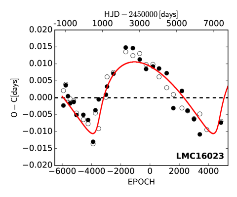
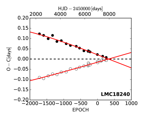
Figure 6: Eclipse timing residual (observed $-$ computed) diagrams for OGLE-LMC-ECL-16023 and 18240 with respect to linear ephemerides listed in Table 13. Black and white points represent primary and secondary minima, respectively. The red line is the best fit of LTE and apsidal motion in the case of OGLE-LMC-ECL-16023 and 18240, respectively.

Table 9: Fitted parameters of the LTE for OGLE-LMC-ECL-16023.

$P_{\rm out}$ [days]	$6495\pm 88$
$T_{0}$ [HJD]	$2418279\pm 482$
$A_{\mathrm{LTE}}$ [days]	$0.01057\pm 0.00066$
$\omega_{1}$ [∘]	$323.0\pm 8.3$
$e_{1}$	$0.711\pm 0.078$

6.2 OGLE-LMC-ECL-18240

OGLE-LMC-ECL-18240 (05:31:33.66 $-$71:14:25.1, I = 17.0 mag) is a detached eclipsing binary, which was found to be also an eccentric one. For this reason, its analysis was a little different. We also included the hypothesis of apsidal motion for the detailed description of its eclipse timing residual diagram analysis (e.g., Gimenez & Garcia-Pelayo, 1983). The effect of apsidal motion also affects the depths of both minima, however, the nodal precession is the most dominant contribution. Moreover, the effect of changing depth in eccentric binaries was properly modelled in our solution using the PHOEBE code. The time coverage is still rather poor and the apsidal motion slow, but the change of the periastron is apparent in the data covering about 15 years. The eccentricity of the inner orbit of the system was found to be of about $0.2$ and the apsidal motion period of 149 yr. The complete solution of apsidal motion is listed in Table 10, where $P_{\mathrm{s}}$ stands for sidereal period. Detailed photometric monitoring in the upcoming years would help us to derive its apsidal parameters with higher confidence. Once this result is achieved, the constrained apsidal motion of the inner binary and the orbital precession may provide more severe limits on the third star mass and its period.

Table 10: Fitted parameters of the apsidal motion for OGLE-LMC-ECL-18240.

$\mathrm{HJD}_{0}$ [HJD]	$2457044.469\pm 0.010$
$P_{\mathrm{s}}$ [days]	$2.764105\pm 0.000014$
$e_{1}$	$0.201\pm 0.076$
$\omega_{1}$ [∘]	$267.5\pm 3.18$
$\mathrm{d}\omega_{1}/\mathrm{d}t$ [∘/cycle]	$0.0183\pm 0.0088$

7 Discussion and conclusions

Multiple stellar systems are important astrophysical laboratories which could help us to understand general mechanisms of mutual N-body dynamic interactions between components, as well as the process of their formation. However, the number of relatively well studied multiple systems still remains low, especially the compact ones manifesting orbital precession. Besides that, results from the Kepler mission show an interesting distribution of orbital periods of triple systems, which is not explained theoretically and more investigation is needed.

In this work, we focused on changing of inclination of eclipsing binaries, and developed new methods, which appear to be suitable for detection of new triples with a small $P_{2}/P_{1}$ ratio. The presented methods led to an identification of 58 new compact triple candidates within the LMC and SMC which is, together with 14 previously known systems, the largest published sample of inclination changing compact triple candidates out of the Milky Way galaxy.

Eight of detected systems were studied thoroughly to determine the basic physical parameters of the eclipsing pair, the third component, and mutual orientation of the orbits. Unfortunately, we found that for precise determination of mutual inclinations a time base of given observations (more than $\approx 20$ years in some cases) is still too short and obtained angles were computed with very large uncertainties. In some cases also $P_{\mathrm{nodal}}$ were computed with large uncertainty, but despite that the systems in our sample still belongs to those with rather small $P_{\mathrm{nodal}}$ (compare Tables 7 and 8 in this work with Table 10 in Borkovits et al. (2016), with a large sample of compact triples discovered by Kepler mission). Our analysis also led to restrictions on the upper limit of possible orbital period $P_{2}$ of the third body. The distribution of the $P_{1}$ and $P_{2}$ with the results of our study are shown in the Fig. 7. One can clearly see that our sample is almost completely located within the area of the lack of triples, as reported by Borkovits et al. (2016). Moreover, periods of some systems in our sample might be close to the limit of stability, which is not determined unambiguously (see Mardling & Aarseth, 2001; Sterzik & Tokovinin, 2002; Tokovinin, 2004, 2007). But new observations with longer time bases, in the ideal case both photometric and spectroscopic, are needed to obtain parameters for all identified triples and to improve the precision of the determined parameters for the eight analyzed systems.

It should be noted that the upper limits on $m_{2}$ and consequently $P_{2}$ are estimated with relatively rough assumptions based on absence of third light in the light curve solutions and the real upper limits might be slightly different. However, it cannot change the fact that systems presented in this paper are most probably within the region with the lack of triples in the $P_{1}-P_{2}$ distribution, and that makes listed systems as perfect targets for a campaign of photometric observations targeting on minima timing with cadence of the order of weeks, which should lead to precise determination of the third body orbital period. Absence of a third light in the light curve solution for all studied systems could seem quite interesting, because it also means that $m_{2}<m_{0}+m_{1}$ but in the Milky Way galaxy the third body mass $m_{2}$ tends to be similar to the mass of eclipsing pair $m_{0}+m_{1}$ and for $81\,\%$ of triples $m_{2}/(m_{0}+m_{1})$ ratio is greater than $0.2$ (Tokovinin, 2008; Correia et al., 2006). Comparison of distributions of triple component masses between the Milky Way galaxy and the Magellanic Clouds with different metalicities could be very interesting and useful for theory of multiple stellar systems formation. But in this case the third light absence is most probably result of selection effects of our methods.

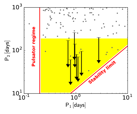
Figure 7: Area with the lack of triples in $P_{1}-P_{2}$ distribution with the systems studied in this work. As only upper limit on $P_{2}$ has been estimated, each system is depicted like an arrow with upper limit. Triples found within the Kepler field are marked with a gray dots.

Appendix A Light curves of EBs with amplitude variation located in the LMC and SMC.

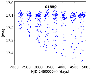
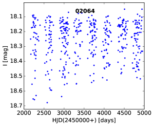
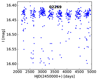
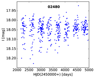
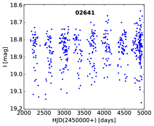
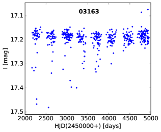
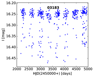
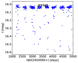
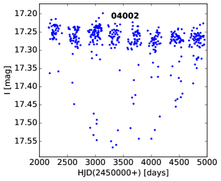
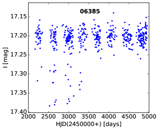
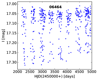
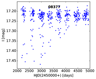
Figure 8: Light curves of EBs with amplitude variation from the OGLE III LMC database.

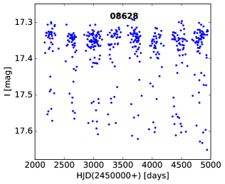
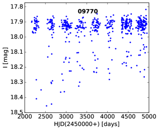
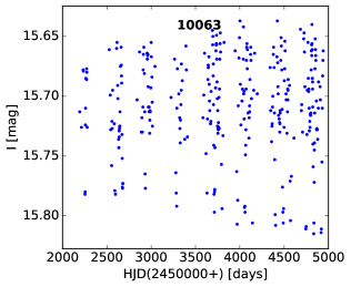
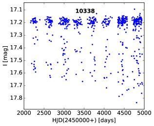
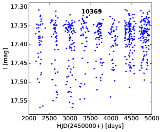
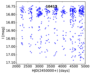
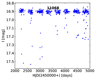
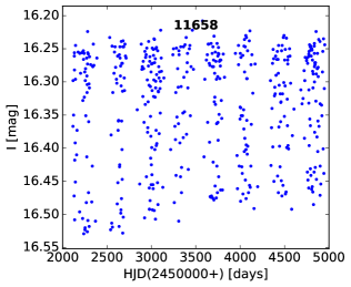
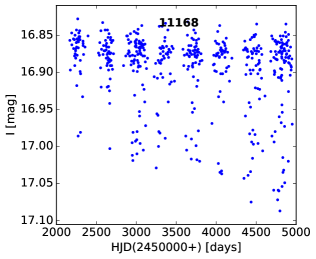
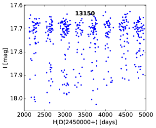
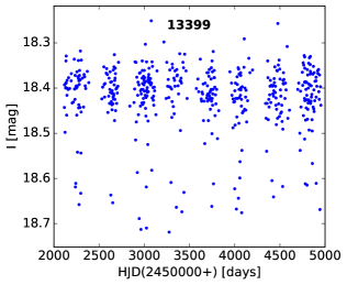
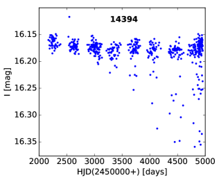
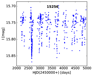
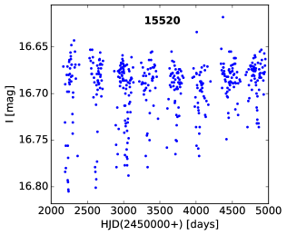
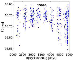
Figure 9: continued

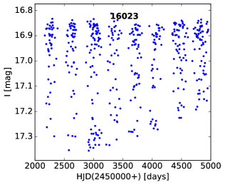
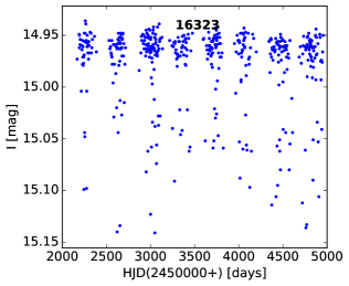
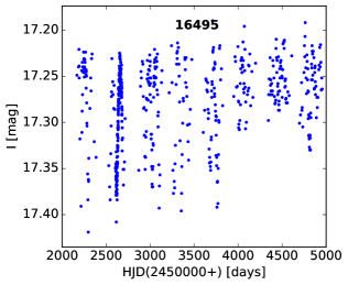
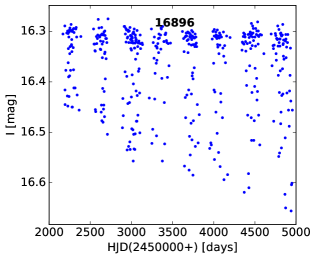
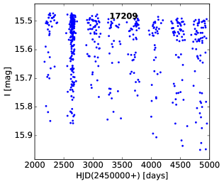
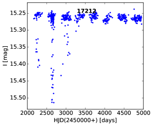
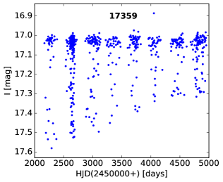
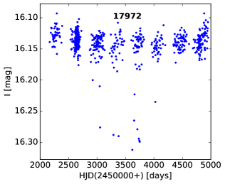
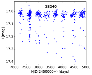
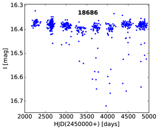
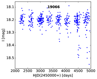
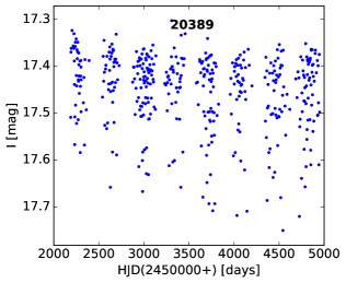
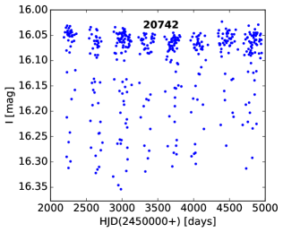
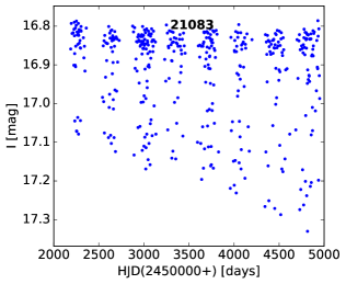
Figure 10: continued

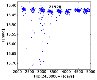
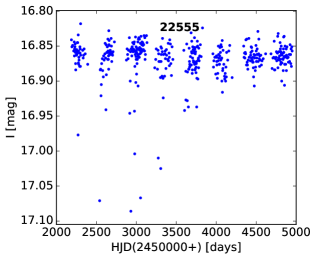
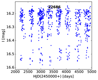
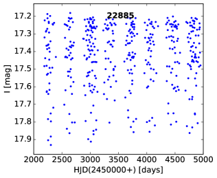
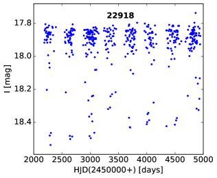
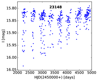
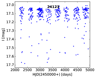
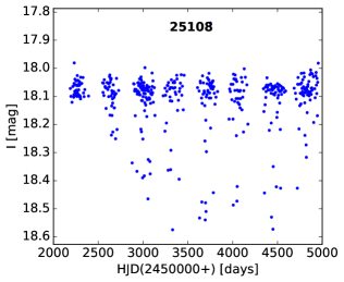
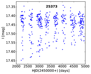
Figure 11: continued

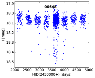
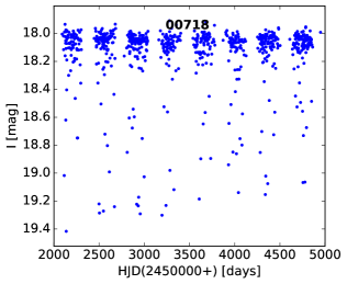
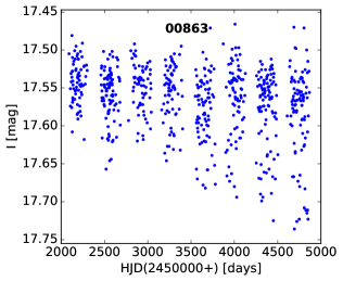
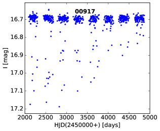
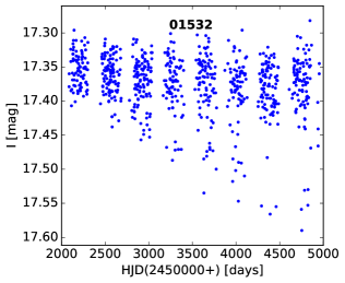
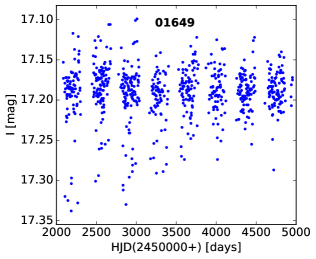
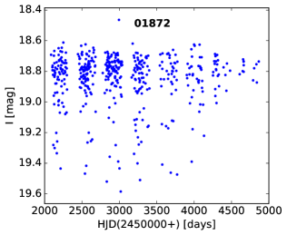
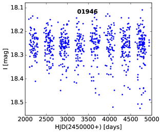
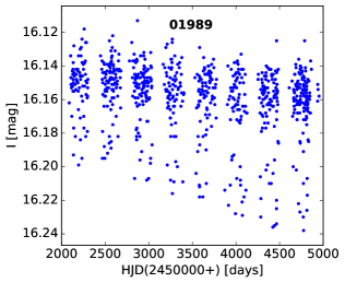
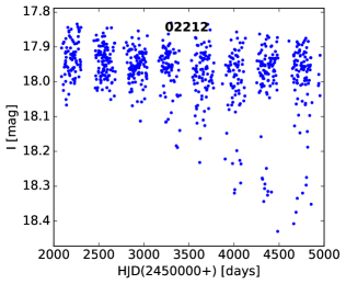
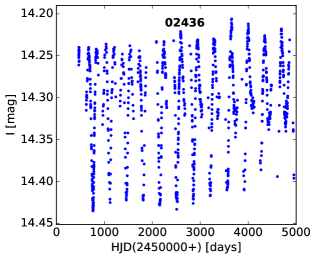
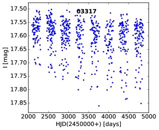
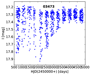
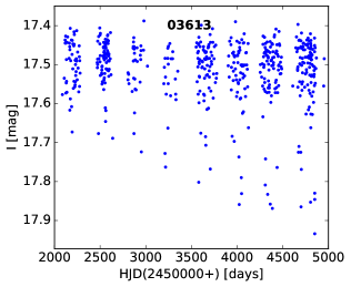
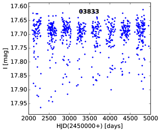
Figure 12: Light curves of EBs with amplitude variation from the OGLE III SMC database.

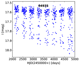
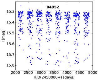
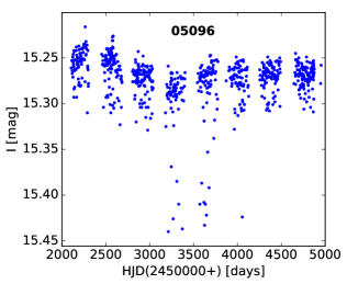
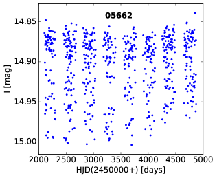
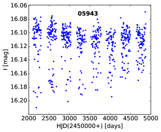
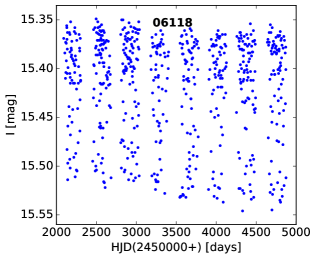
Figure 13: continued

Appendix B Photometric solutions for selected eclipsing binaries in the LMC and SMC

Table 11: Eclipsing binaries in the LMC.

OGLE-LMC-ECL-	01350	13150	16023	18240	23148
Parameter
$T_{0}\,\mathrm{(K)}$ (fixed)	$13000$	$11000$	$14000$	$17000$	$28000$
$T_{1}\,\mathrm{(K)}$	$12612$	$10984$	$13482$	$13075$	$22985$
$i_{0}\,(^{\circ})$	$67.2-77.4$	$65.3-81.1$	$48.8-75.7$	$92.8-97.8$	$<60.0-72.1$
$q=m_{1}/m_{0}$	$1.0$ (fixed)	$1.0$ (fixed)	$1.0$ (fixed)	$1.0$ (fixed)	$0.78$
$R_{0}/a_{1}$	$0.26$	$0.27$	$0.37$	$0.17$	$0.27$
$R_{1}/a_{1}$	$0.30$	$0.29$	$0.37$	$0.11$	$0.27$
$M_{\rm bol0}$ (mag)	$-0.83$	$-0.2$	$-1.9$	$-1.1$	$-4.3$
$M_{\rm bol1}$ (mag)	$-1.01$	$-0.4$	$-1.8$	$-1.0$	$-3.4$
$L_{\rm V0}$ (%)	…	$45.4$	$51.6$	…	$58.1$
$L_{\rm V1}$ (%)	…	$54.7$	$48.4$	…	$41.9$
$L_{\rm R0}$ (%)	…	$45.4$	$51.4$	…	$57.6$
$L_{\rm R1}$ (%)	…	$54.6$	$48.6$	…	$42.4$
$L_{\rm I0}$ (%)	$43.9$	$45.3$	$51.4$	$78.0$	$57.0$
$L_{\rm I1}$ (%)	$56.1$	$54.7$	$48.6$	$22.0$	$43.0$

Table 12: Eclipsing binaries in the SMC.

OGLE-SMC-ECL-	1532	3317	6118
Parameter
$T_{0}\,\mathrm{(K)}$ (fixed)	$16500$	$16000$	$26000$
$T_{1}\,\mathrm{(K)}$	$6373$	$5397$	$25906$
$i_{0}\,(^{\circ})$	$<55.0-68.1$	$<53.0-66.1$	$60.6-62.3$
$q=m_{1}/m_{0}$	$0.3$	$0.25$	$1.0$ (fixed)
$R_{0}/a_{1}$	$0.36$	$0.49$	$0.33$
$R_{1}/a_{1}$	$0.23$	$0.25$	$0.34$
$M_{\rm bol0}$ (mag)	$-2.5$	$-3.13$	$-4.39$
$M_{\rm bol1}$ (mag)	$2.18$	$3.08$	$-4.42$
$L_{\rm V0}$ (%)	…	…	…
$L_{\rm V1}$ (%)	…	…	…
$L_{\rm R0}$ (%)	$92.8$	…	…
$L_{\rm R1}$ (%)	$2.2$	…	…
$L_{\rm I0}$ (%)	$90.2$	$97.3$	$49.0$
$L_{\rm I1}$ (%)	$9.8$	$2.7$	$51.0$

Appendix C Ephemerides for analyzed eclipsing binaries

Table 13: Ephemerides for the LMC eclipsing binaries.

OGLE-LMC-ECL-	Time interval (HJD)	HJD0	$P_{1}$ (days)
01350	whole	2456308.2933(10)	1.09883233(21)
13150	whole	2453541.39142(97)	0.95597619(38)
16023	2448896.0883 ¡ HJD ¡ 2450389.1889	2453562.506(10)	0.7882459(20)
	2450389.1889 ¡ HJD ¡ 2452484.4118	2453562.5692(88)	0.7882625(28)
	2452484.4118 ¡ HJD ¡ 2457389.4966	2453562.5422(13)	0.78824656(69)
	whole	2453562.5333(23)	0.78825063(63)
18240	whole	2457044.4687(72)	2.7641050(60)
23148	whole	2443568.0121(59)	1.28218324(86)

Table 14: Ephemerides for the SMC eclipsing binaries.

OGLE-SMC-ECL-	Time interval (HJD)	HJD0	$P_{1}$ (days)
1532	whole	2455000.4915(34)	1.0283876(18)
3317	whole	2455000.4583(21)	0.70421606(63)
6118	whole	2455000.5435(25)	0.9372806(15)

Appendix D Solutions of the time dependencies of inclination for selected systems

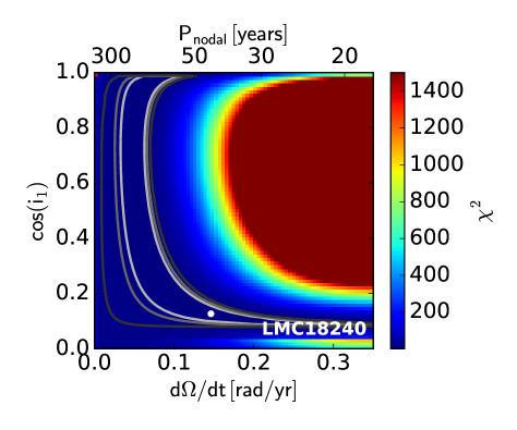
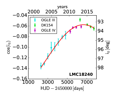
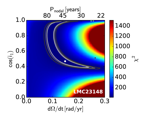
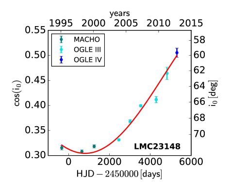
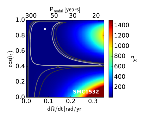
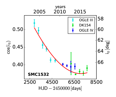
Figure 15: continued

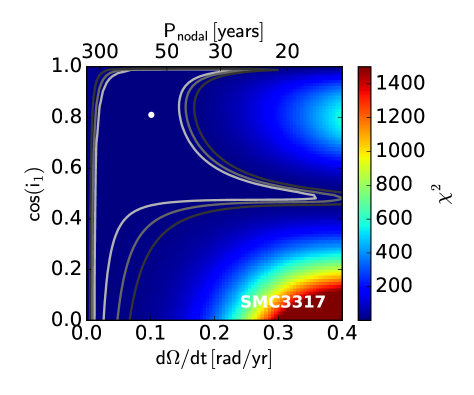
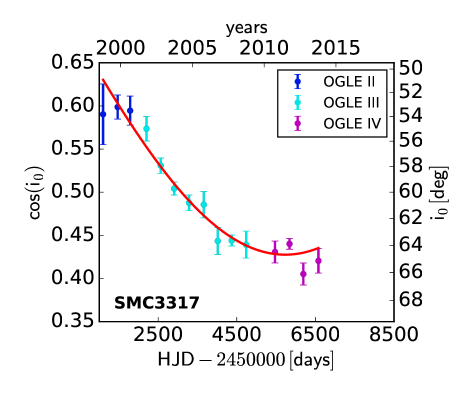
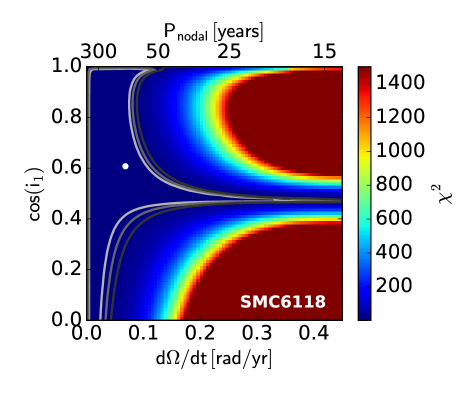
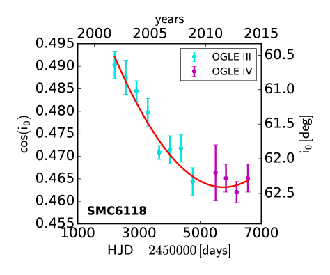
Figure 16: continued

Appendix E Possible masses and periods of third bodies

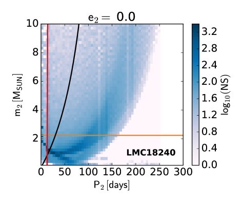
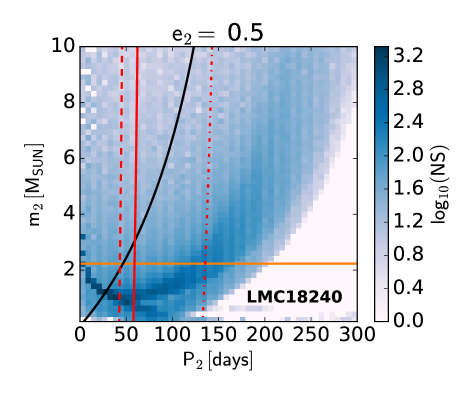
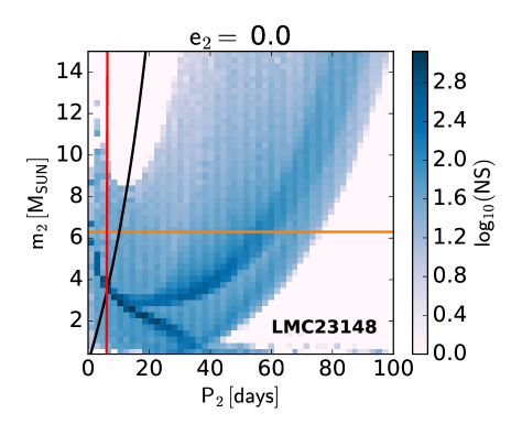
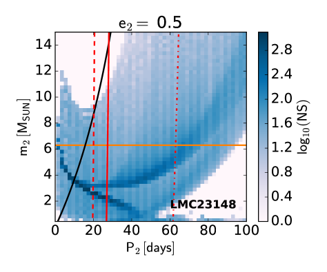
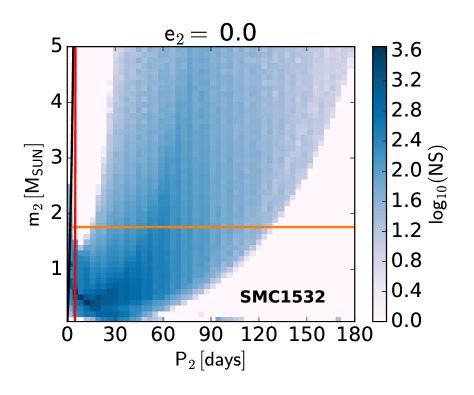
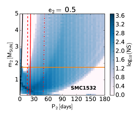
Figure 18: (Continued from the previous page.) Red solid line indicates the stability limit according to (Mardling & Aarseth 2001), dashed line indicates the stability limit according to (Sterzik & Tokovinin 2002) and dot-dashed line according to (Tokovinin 2004). The blue line shows restrictions on ETVs. All figures are plotted for the extremal third body eccentricities $e_{2}=0$ and $e_{2}=0.5$.

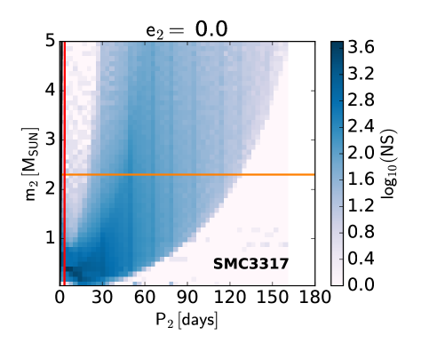
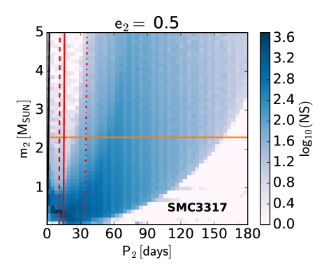
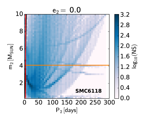
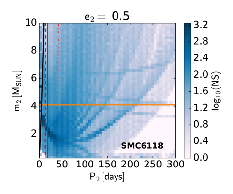
Figure 19: continue

Appendix F Eclipse timing residual diagrams

Appendix G Light curves of selected systems

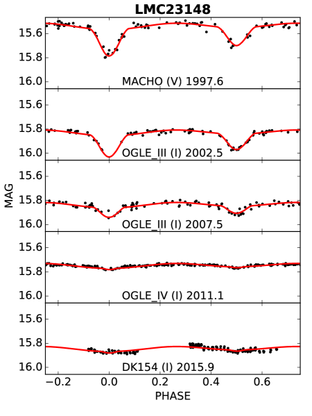
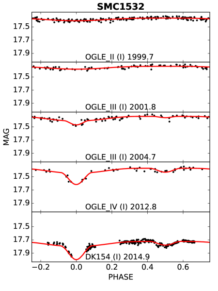
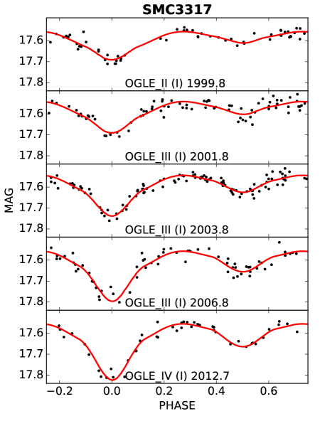
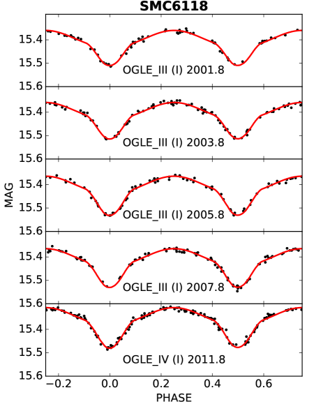
Figure 22: continue

Appendix H Definition of symbols

Table 15: Definition of symbols.

	Parameter	Symbol
Mass
	Inner binary components	$m_{0}$, $m_{1}$
	Third body	$m_{2}$
	Total mass of the inner binary	$M_{1}$
	Total mass of the system	$M_{2}$
	Mass ratio of inner binary components	$q$
Eccentricity	Inner and outer orbit	$e_{1}$, $e_{2}$
Seminajor axis	Inner and outer orbit	$a_{1}$, $a_{2}$
Orbital angular momentum	Inner and outer orbit	$l_{1}$, $l_{2}$
Argument of periastron	Inner and outer orbit	$\omega_{1}$, $\omega_{2}$
Angular velocity	Nodal line precession	$\dot{\Omega}$
Period
	Orbital period of the inner binary	$P_{1}$
	Orbital period of the third component	$P_{2}$
	Sidereal period of the inner binary	$P_{\mathrm{s}}$
	Nodal line precession	$P_{\mathrm{nodal}}$
Inclination
	Observable inclination of the inner binary	$i_{0}$
	Angles between the invariant plane and the orbits	$i_{1}$, $i_{2}$
	Observable inclination of the third body	$i_{3}$, $i_{\mathrm{3,inv}}$
	Angle between invariant plane and plane tangent to the celestial sphere	$I$
	Mutual inclination of inner and outer orbit	$j$
Reference epochs
	Reference minimum of eclipsing binary	HJD0
	Periastron passage	$T_{0}$
	Passage nodal line through the plane tangent to the celestial sphere	$t_{0}$
Photometric solution
	Relative radii of EB components with respect to the semimajor axis	$R_{0}/a_{1}$, $R_{1}/a_{1}$
	Temperatures of primary and secondary component	$T_{1}$, $T_{2}$
	Relative luminosities of primary and secondary component	$L_{\mathrm{X0}}$, $L_{\mathrm{X1}}$
	Bolometric magnitudes of primary and secondary component	$M_{\mathrm{bol0}}$, $M_{\mathrm{bol1}}$
Amplitude of ETVs
	Dynamical delay	$A_{\mathrm{phys}}$
	Røemer’s delay	$A_{\mathrm{LTE}}$