Cross-modal Recurrent Models for Weight Objective
Prediction from Multimodal Time-series Data

Abstract

We analyse multimodal time-series data corresponding to weight, sleep and steps measurements. We focus on predicting whether a user will successfully achieve his/her weight objective. For this, we design several deep long short-term memory (LSTM) architectures, including a novel cross-modal LSTM (X-LSTM), and demonstrate their superiority over baseline approaches. The X-LSTM improves parameter efficiency by processing each modality separately and allowing for information flow between them by way of recurrent cross-connections. We present a general hyperparameter optimisation technique for X-LSTMs, which allows us to significantly improve on the LSTM and a prior state-of-the-art cross-modal approach, using a comparable number of parameters. Finally, we visualise the model’s predictions, revealing implications about latent variables in this task.

1 Introduction

Recently, consumer-grade health devices, such as wearables and smart home appliances became more widespread, which presents new data modelling opportunities. Here, we investigate one such task—predicting the users’ future body weight in relation to their weight goal given historical weight, and sleep and steps measurements. This study is enabled by a first-of-its-kind dataset of fitness measurements from $\sim$15000 users. Data are captured from different sources, such as smartwatches, wrist- and hip-mounted wearables, smartphone applications and smart bathroom scales.

In this work, we show that that deep long short-term memory (LSTM) [7] models are able to produce accurate predictions in this setting, significantly outperforming baseline approaches, even though some factors are only observed latently. We also discover interesting patterns in input sequences that push the network’s confidence in success or failure to extremes. We hypothesise that these patterns affect latent variables and link our hypotheses to existing research on sleep.

Most importantly, we improve the parameter efficiency of LSTM models for multimodal input (in this case sleep/steps/weight measurements) by proposing cross-modal LSTMs (X-LSTMs). X-LSTMs extract features from each modality separately, while still allowing for information flow between the different modalities by way of cross-connections. Our findings are supported by a general data-driven methodology (applicable to arbitrary multimodal problems) that exploits unimodal predictive power to vastly simplify finding appropriate hyperparameters for X-LSTMs (reducing most of the tuning effort to a single parameter). We also compare our model to a previous state-of-the-art cross-modal sequential data technique [17], outlining its limitations and successfully outperforming it on this task.

2 Dataset and Preprocessing

We performed our investigation on anonymised data obtained from bathroom scales and wearables of the Nokia Digital Health - Withings range, gathered using the Withings smartphone application.

The data was pre-processed to remove outliers or users with too few, or too sporadic, data observations. We consider a weight objective achieved if there exists a weight measurement in the future that reaches or exceeds it, and failed if the user stops recording weights (allowing for a long enough window after the end of the recorded sequence) or sets a more conservative objective. Following best practices, data are normalised to have mean zero and standard deviation one per-feature.

The derived dataset spans 18036 sequences associated with weight objectives. All of the sequences are comprised of user-related features: height, gender, age category, weight objective and whether it was achieved; along with sequential features—for each day: duration of light and deep sleep, time to fall asleep and time spent awake; number of times awoken during the night; time required to wake up; bed-in/bed-out times; steps and (average) weights for the day. We consider sequences that span at least 10 contiguous days. The dataset contains 6313 successful and 11723 unsuccessful examples.

3 Models under consideration

3.1 Baseline models

We compared deep recurrent models against several common baseline approaches to time-series classification, as outlined in [23]. We considered: Support Vector Machines (SVMs) with the RBF kernel, Random Forests (RFs), Gaussian Hidden Markov Models (GHMMs) and (feedforward) Deep Neural Networks (DNNs). The hyperparameters have been optimised using a thorough sweep.

3.2 Long short-term memory

Our models are based on the LSTM [7] model, defined as follows for a single cell (similar to [5]):

$$i_{t} = \tanh({\bf W}^{\mathrm{xi}}x_{t}+{\bf W}^{\mathrm{yi}}y_{t-1}+b^{\mathrm{i}})$$ (1)

$$\{j,f,o\}_{t} = \tilde{\sigma}({\bf W}^{\mathrm{x\{j,f,o\}}}x_{t}+{\bf W}^{\mathrm{y\{j,f,o\}}}y_{t-1}+b^{\mathrm{\{j,f,o\}}})$$ (2)

$$c_{t} = c_{t-1}\otimes f_{t}+i_{t}\otimes j_{t}$$ (3)

$$y_{t} = \tanh(c_{t})\otimes o_{t}$$ (4)

Here, $\bf W^{*}$ and $b^{*}$ correspond to weights and biases of the LSTM layer, respectively, and $\otimes$ corresponds to element-wise vector multiplication. $\tanh$ is the hyperbolic tangent, and $\tilde{\sigma}$ is the hard sigmoid function. For the remainder of the description, we compress Eqn-s 14–19 into $\mathrm{LSTM}(\vec{x})=\vec{y}$.

Our primary architecture is a 3-layer LSTM model (21, 42 and 84 features) for processing the sequential data. The features computed by the final LSTM layer are concatenated with the height, gender, age category and weight objective, providing the following feature representation:

$$\mathrm{LSTM}(\mathrm{LSTM}(\mathrm{LSTM}(\vec{\mathrm{wt}}||\vec{\mathrm{sl}}||\vec{\mathrm{st}})))_{T}||\mathrm{ht}||\mathrm{gdr}||\mathrm{age}||\mathrm{obj}$$ (5)

where $\vec{\mathrm{wt}}$, $\vec{\mathrm{sl}}$ and $\vec{\mathrm{st}}$ are the input features (for weight, sleep and steps, respectively), $||$ is featurewise concatenation, and $T$ is the length of the initial sequence. The result is processed by a 3-layer fully-connected network (128, 64, 1 neurons) with logistic sigmoid activation at the very end.

3.3 Cross-modal LSTM (X-LSTM)

For this task we also propose a novel cross-modal LSTM (X-LSTM) architecture which exploits the multimodality of the input data explicitly, while using the same number of parameters as the traditional LSTM. We partition the input sequence into three parts (sleep, weight and steps data), and pass each of those through a separate three-layer LSTM stream. We also allow for information flow between the streams in the second layer, by way of cross-connections, where features from a single sequence stream are passed and concatenated with features from another sequence stream (after being passed through an additional LSTM layer). In equation form, outputs of the three streams are:

$$\vec{h}^{\mathrm{\{wt,sl,st\}}}_{1} = \mathrm{LSTM}(\{\vec{\mathrm{wt}},\vec{\mathrm{sl}},\vec{\mathrm{st}}\})$$ (6)

$$\vec{h}^{\mathrm{\{wt\rightarrow wt,sl\rightarrow sl,st\rightarrow st\}}}_{2} = \mathrm{LSTM}(\{\vec{h}^{\mathrm{wt}}_{1},\vec{h}^{\mathrm{sl}}_{1},\vec{h}^{\mathrm{st}}_{1}\})$$ (7)

$$\vec{h}^{\mathrm{\{wt\rightsquigarrow sl,wt\rightsquigarrow st\}}}_{2} = \mathrm{LSTM}(\{\vec{h}^{\mathrm{wt}}_{1},\vec{h}^{\mathrm{wt}}_{1}\})$$ (8)

$$\vec{h}^{\mathrm{\{sl\rightsquigarrow wt,sl\rightsquigarrow st\}}}_{2} = \mathrm{LSTM}(\{\vec{h}^{\mathrm{sl}}_{1},\vec{h}^{\mathrm{sl}}_{1}\})$$ (9)

$$\vec{h}^{\mathrm{\{st\rightsquigarrow wt,st\rightsquigarrow sl\}}}_{2} = \mathrm{LSTM}(\{\vec{h}^{\mathrm{st}}_{1},\vec{h}^{\mathrm{st}}_{1}\})$$ (10)

$$\vec{h}^{\mathrm{wt}}_{3} = \mathrm{LSTM}(\vec{h}^{\mathrm{wt\rightarrow wt}}_{2}||\vec{h}^{\mathrm{sl\rightsquigarrow wt}}_{2}||\vec{h}^{\mathrm{st\rightsquigarrow wt}}_{2})$$ (11)

$$\vec{h}^{\mathrm{sl}}_{3} = \mathrm{LSTM}(\vec{h}^{\mathrm{sl\rightarrow sl}}_{2}||\vec{h}^{\mathrm{wt\rightsquigarrow sl}}_{2}||\vec{h}^{\mathrm{st\rightsquigarrow sl}}_{2})$$ (12)

$$\vec{h}^{\mathrm{st}}_{3} = \mathrm{LSTM}(\vec{h}^{\mathrm{st\rightarrow st}}_{2}||\vec{h}^{\mathrm{wt\rightsquigarrow st}}_{2}||\vec{h}^{\mathrm{sl\rightsquigarrow st}}_{2})$$ (13)

We used $\vec{h}^{\{x,y,z\}}_{2}=\mathrm{LSTM}(\{a,b,c\})$ to denote $\vec{h}^{x}_{2}=\mathrm{LSTM}(a),\vec{h}^{y}_{2}=\mathrm{LSTM}(b),\vec{h}^{z}_{2}=\mathrm{LSTM}(c)$.

Finally, the final LSTM frames across all of the three streams are concatenated before being passed on to the fully-connected classifier: $(\vec{h}^{\mathrm{wt}}_{3}||\vec{h}^{\mathrm{sl}}_{3}||\vec{h}^{\mathrm{st}}_{3})_{T}||\mathrm{ht}||\mathrm{gdr}||\mathrm{age}||\mathrm{obj}$.

The illustration of the entire construction process from individual building blocks is shown in Fig. 1. Similar techniques have already been successfully applied for handling sparsity within convolutional neural networks [22] and audiovisual data integration [2]. We evaluate three cross-connecting strategies: one given by Eqn-s 21–27 (A), one where cross-connections do not have intra-layer LSTMs (B), and one without cross-connections (N). The latter corresponds to prior work on multimodal deep learning [15, 21] and allows for computing the largest number of features within the parameter budget out of all three variants—no parameters are spent on cross-connections.

Finally, we consider a recent state-of-the-art approach for processing multimodal sequential data [17] which imposes cross-modality via weight sharing ($\mathbf{W}^{y*}$ in Eqn-s 14–17)—we refer to this method as SH-LSTM. This hinders expressivity—in order to share the weights, the matrices to have be of the same size, requiring all modality streams to compute the same number of features at each depth level. Keeping the parameter count comparable to the baseline LSTM, we evaluate three strategies for weight sharing: sharing across all modalities (ALL) and sharing only across weight & sleep, with (WSL) and without (CUT) steps data. This has been informed by the fact that the weight and sleep data have, on their own, been found to be significantly more influential than steps data.

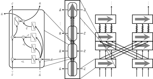
Figure 1: A diagram of a 3-layer X-LSTM model and one cross-connection in the second layer. Left: A single LSTM block, Middle: An LSTM layer (replicated cell). Right: A 3-layer cross-modal LSTM model with 2 streams. In the second layer, the hidden sequences are passed through a separate LSTM layer and feature-wise concatenated with the main stream sequence to facilitate sharing.

3.4 X-LSTM hyperparameter tuning

In practice, we anticipate X-LSTMs to be derived from a baseline LSTM, in order to redistribute its parameters more efficiently. However, X-LSTMs might introduce an overwhelming amount of hyperparameters to tune. To make the process less taxing, we focus on the meaning of the feature counts—their comparative values are supposed to track the relative significance of each modality. First, we attempt to solve the task with a basic LSTM architecture using only one of the modalities. When scores (e.g. accuracies or AUC) $s_{wt},s_{sl}$ and $s_{st}$ are obtained for all three modalities, we redistribute the intra-layer feature counts of the X-LSTM according to the ratio $s_{wt}:s_{sl}:s_{st}$.

To enforce larger discrepancies, we raise the obtained scores to a power $k$. This controls the tendency of the network to favour the most predictive modality when redistributing features. For a fixed choice of $k$, we solve a system of equations in order to derive feature counts for all the intra-layer LSTM layers in an X-LSTM. Thus, most of the effort amounts to finding just one hyperparameter—$k$.

4 Results

4.1 Weight objective success classification

We performed stratified 10-fold crossvalidation on the baseline classifiers and the proposed LSTM models. We use ROC curves (and the AUC) as our evaluation metric, but we also report the accuracy, precision, recall, F₁ score and the MCC [12] for the threshold which maximises the F₁ score.

To construct competitive X-LSTMs, we computed the AUCs of the individual unimodal LSTMs on a validation dataset. The results were too similar to reliably generate non-uniform X-LSTMs, so we searched for parameter $k$. The X-LSTM performed the best with $k=30$, and (B) cross-connections (75089 parameters)—we compare it directly with the LSTM (76377 parameters) and the SH-LSTMs.

To confirm that the advantages of our methodology are statistically significant, we have performed paired $t$-testing on the metrics of individual cross-validation folds, choosing a significance threshold of $p<0.05$. The SH-LSTM performed the best in its (WSL) variant but even then was unable to outperform the baseline LSTM—highlighting how essential is the ability to accurately specify relative importances between modalities. The results are summarised in Table 3.

Metric	SVM	RF	GHMM	DNN	LSTM	SH-LSTM	X-LSTM
Accuracy	67.65%	70.97%	66.31%	68.93%	79.12%	78.49%	80.30%
Precision	52.54%	56.05%	51.26%	53.80%	67.25%	65.31%	68.66%
Recall	81.02%	81.34%	82.32%	83.02%	79.30%	82.95%	81.62%
F1 score	63.71%	66.25%	63.11%	65.18%	72.69%	72.98%	74.37%
MCC	39.74%	44.75%	38.57%	42.63%	56.60%	56.80%	59.45%
ROC AUC	76.77%	79.97%	74.86%	78.54%	86.91%	86.63%	88.07%
$p$-value	$2\cdot 10^{-12}$	$6\cdot 10^{-10}$	$7\cdot 10^{-11}$	$2\cdot 10^{-11}$	$1\cdot 10^{-4}$	$4\cdot 10^{-5}$	—

Table 1: Comparative evaluation results of the baseline models against the LSTMs after 10-fold crossvalidation. Reported X-LSTM is (B) with $k=30$ and SH-LSTM is (WSL). Reported $p$-values are for the X-LSTM vs. each baseline for the ROC-AUC metric.

4.2 Visualising detected features

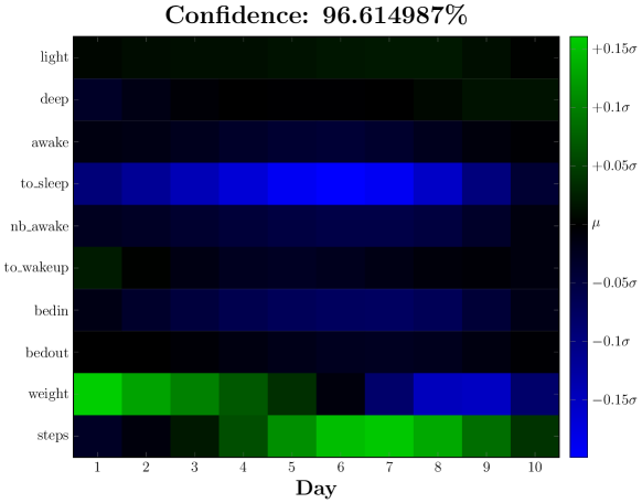
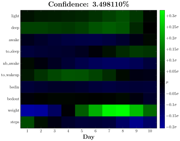
Figure 2: Iteratively produced artificial sequences that maximise the model’s confidence in achieving (left) or failing (right) a $-4\mathrm{kg}$ weight objective. Best viewed in colour.

It is hard to interpet the parameters of a network directly, so instead we focus on generating artificial sequences that maximise the network’s confidence in success or failure [19]. Iteratively, we produce an input $\mathbf{I^{\prime}}$ that maximises the network’s confidence, starting from $\mathbf{I}_{0}=\mathbf{0}$: $\mathbf{I^{\prime}}=\operatorname*{argmax}_{\mathbf{I}}\Sigma(\mathbf{I})-\lambda||\mathbf{I}||^{2}_{2}$ where $\Sigma(\mathbf{I})$ is the network’s output for $\mathbf{I}$, and $\lambda$ is an $L_{2}$-regularisation parameter (to penalise large day-to-day variances). We found that $\lambda=5$ works best.

Generated sequences spanning 10 days are shown in Fig. 2. As expected, we observe that a user is likely to hit their weight objective if there is a downwards the trend in weight and an upwards trend in steps, and vice-versa for a failing sequence. Interestingly, the model also uncovered that to have a higher confidence of success, it is important for the user to fall asleep quicker once going to bed. This is likely encoding important latent variables that we can not directly access from the dataset—for example, a person that takes more time to fall asleep is more likely to snack in the evening, which is known to be detrimental to weight loss (as previously observed in biomedical research [14, 18, 11]).

Appendix A Appendices to sections

In the following sections, we augment the exposition of the main body of our paper to include further relevant details—for the purposes of gaining a better understanding of the utilised dataset, the implemented models, and the presented results.

A.1 Dataset and preprocessing

We performed our investigation on anonymised data obtained from several devices across the Nokia Digital Health - Withings range. The dataset contains weight, height, sleep and steps measurements, as well as user specified weight objectives. Weights are measured by the Withings scale. All other data are obtained from the Withings application through the use of wearables.

Users were first included in the dataset under the condition of having recorded at least 10 weight measurements over a 2-month period. In total, the dataset contains 1 664 877 such users. Further processing was performed to remove outliers or those users with too few, or too sporadic, data observations; after this stage $\sim$ 15K users were remaining. The precise steps taken to reach this final dataset are enumerated below.

Obvious outliers, reporting unrealistic heights (below 130cm or above 225cm), and/or consistent weight changes of more than 1.5kg per day have been discarded. Steps and sleep are recorded on a per-day basis, while weights are recorded at the user’s discretion; to align the weight measurements with the other two modalities, we have applied a moving average to the person’s recorded weight throughout an individual day. A sequence may be labelled with any weight objective that has been set by the user, and is still unachieved, by the time the sequence ends. Overly ambitious objectives (over $\pm$20 kilograms proposed) are ignored. We consider a weight objective successful if there exists a weight measurement in the future that reaches or exceeds it, and we consider it unsuccessful if the user stops recording weights (allowing for a long enough window after the end of the recorded sequence) or sets a more conservative objective in the meantime. In line with known best practices in deep learning, data are normalised to have mean zero and standard deviation one per-feature.

The derived dataset spans 18036 sequences associated with weight objectives. All of the sequences are comprised of user-related features: height, gender, age category, weight objective; along with sequential features—for each day: duration of light and deep sleep, time to fall asleep and time spent awake; number of times awoken during the night; time required to wake up; bed-in/bed-out times; steps and (average) weights for the day. We consider sequences that span at least 10 contiguous days.

Every sequence also has a boolean label, indicating whether the objective has been successfully achieved at some point in the future. Within our dataset, 6313 of the sequences represent successful examples, while the remaining 11723 represent examples of failure. To address the potential issues of class imbalance, appropriate class weights are applied to all optimisation targets and loss functions.

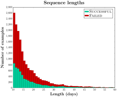
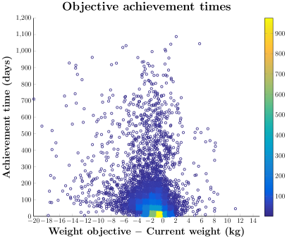
Figure 3: Left: Plot of the sequence length distribution in the final dataset. Right: Mixed heatmap/scatter plot of the weight objectives against their achievement times, for the successful sequences in the final dataset.

In order to get an impression of the statistics present within the dataset, we have generated plots of the sequence length distributions (outliers removed for visibility), as well as scatter plots of successful weight objective magnitudes against their achievement times. These are provided by Figure 3.

We perform a task of probabilistic classification on the filtered dataset: predicting success for the weight objective, evaluated using crossvalidation (this corresponds to a typical binary classification problem).

A.2 Baseline models

In order to ascertain the suitability of deep recurrent models on this task, we have compared them on the objective classification task against several common baseline approaches to time-series classification, as outlined in [23]. For this purpose, we have considered four such models: Support Vector Machines (SVMs) using the RBF kernel, Random Forests (RFs), Gaussian Hidden Markov Models (GHMMs) and (feedforward) Deep Neural Networks (DNNs). The hyperparameters associated with the baseline models have been optimised with a thorough hyperparameter sweep—on a separate validation set—as detailed below.

For the SVM, we have performed a grid search on its two hyperparameters ($C$ and $\gamma$) in the range $\gamma\in 2^{[-15,5]},C\in 2^{[-5,15]}$, finding the values of $\gamma=2^{-13}$ and $C=2^{9}$ to work best. For the RF, we have performed a search on the number of trees to use in the range $N\in[10,100]$, finding $N=50$ to work best. For the GHMM, we have performed a search on the number of nodes to use in the range $N\in[3,40]$, finding $N=7$ to work best. For the DNN, we have optimised the number of hidden layers (keeping the number of parameters comparable to the recurrent models) in the range $\ell\in[1,10]$, finding $\ell=5$ to work best. This implied that each hidden layer had $N=120$ neurons. All hidden layers apply the rectified linear (ReLU) activation [13], and are regularised using batch normalisation [8] and dropout [20] with $p=0.5$. All other relevant hyperparameters (such as the SGD optimiser and batch size) are the same as for the recurrent models.

For all the non-sequential models (SVM, RF, DNN), we have performed a search on the number of most recent time steps to use in the range $l\in[5,100]$, finding $l=10$ to perform the best. The SVM model has been augmented to produce probabilistic predictions (and thus enable its ROC-AUC metric to be computed) by leveraging Platt scaling [16].

A.3 Long short-term memory

All of our models are based on the long short-term memory (LSTM) [7] recurrent model. The equations describing a single LSTM cell that we employed (similar to [5]) are as follows:

$$i_{t} = \tanh({\bf W}^{\mathrm{xi}}x_{t}+{\bf W}^{\mathrm{yi}}y_{t-1}+b^{\mathrm{i}})$$ (14)

$$j_{t} = \tilde{\sigma}({\bf W}^{\mathrm{xj}}x_{t}+{\bf W}^{\mathrm{yj}}y_{t-1}+b^{\mathrm{j}})$$ (15)

$$f_{t} = \tilde{\sigma}({\bf W}^{\mathrm{xf}}x_{t}+{\bf W}^{\mathrm{yf}}y_{t-1}+b^{\mathrm{f}})$$ (16)

$$o_{t} = \tilde{\sigma}({\bf W}^{\mathrm{xo}}x_{t}+{\bf W}^{\mathrm{yo}}y_{t-1}+b^{\mathrm{o}})$$ (17)

$$c_{t} = c_{t-1}\otimes f_{t}+i_{t}\otimes j_{t}$$ (18)

$$y_{t} = \tanh(c_{t})\otimes o_{t}$$ (19)

In these equations, $\bf W^{*}$ and $b^{*}$ correspond to learnable parameters (weights and biases, respectively) of the LSTM layer, and $\otimes$ corresponds to element-wise vector multiplication. $\tanh$ is the hyperbolic tangent function, and $\tilde{\sigma}$ is the hard sigmoid function. To aid clarity, for the remainder of the model description, we will compress Equations 14–19 into $\mathrm{LSTM}(\vec{x})=\vec{y}$, representing a single LSTM layer, with its internal parameters and memory cell state kept implicit.

Our primary architecture represents a three-layer deep LSTM model for processing the historical weight/sleep/steps data. After performing the LSTM operations, the features of the final computed LSTM output step are concatenated with the height, gender, age category and weight objective, providing the following feature representation:

$$\mathrm{LSTM}(\mathrm{LSTM}(\mathrm{LSTM}(\vec{\mathrm{wt}}||\vec{\mathrm{sl}}||\vec{\mathrm{st}})))_{T}||\mathrm{ht}||\mathrm{gdr}||\mathrm{age}||\mathrm{obj}$$ (20)

where $\vec{\mathrm{wt}}$, $\vec{\mathrm{sl}}$ and $\vec{\mathrm{st}}$ are the input features (for weight, sleep and steps, respectively), $||$ corresponds to featurewise concatenation, and $T$ is the length of the initial sequence. These features are passed through two fully connected neural network layers, connected to a single output neuron which utilises a logistic sigmoid activation.

The fully connected layers of the networks apply rectified linear (ReLU) activations. We initialise the LSTM weights using Xavier initialisation [4], and its forget gate biases with ones [9]. Finally, the fully connected weights are initialised using He initialisation [6], as recommended for ReLUs. The models are trained for 200 epochs using the Adam SGD optimiser, with hyperparameters as described in [10], and a batch size of 1024. For regularisation purposes, we have applied batch normalisation to the output of every hidden layer and dropout with $p=0.1$ to the input-to-hidden transitions within the LSTMs [25].

A.4 Cross-modal LSTM

For this task we also propose a novel cross-modal LSTM (X-LSTM) architecture which exploits the multimodality of the input data more explicitly in order to efficiently redistribute the LSTM’s parameters. We initially partition the input sequence into three parts (sleep data, weight data, steps data), and pass each of those through a separate three-layer LSTM stream. We also allow for information flow between the streams in the second layer, by way of cross-connections, where features from a single sequence stream are passed and concatenated with features from another sequence stream (after being passed through an additional LSTM layer). Represented via equations, the computed outputs across the three streams are:

$$\vec{h}^{\mathrm{wt}}_{1} =\mathrm{LSTM}(\vec{\mathrm{wt}}) \vec{h}^{\mathrm{sl}}_{1} =\mathrm{LSTM}(\vec{\mathrm{sl}}) \vec{h}^{\mathrm{st}}_{1} =\mathrm{LSTM}(\vec{\mathrm{st}})$$ (21)

$$\vec{h}^{\mathrm{wt\rightarrow wt}}_{2} =\mathrm{LSTM}(\vec{h}^{\mathrm{wt}}_{1}) \vec{h}^{\mathrm{sl\rightarrow sl}}_{2} =\mathrm{LSTM}(\vec{h}^{\mathrm{sl}}_{1}) \vec{h}^{\mathrm{st\rightarrow st}}_{2} =\mathrm{LSTM}(\vec{h}^{\mathrm{st}}_{1})$$ (22)

$$\vec{h}^{\mathrm{wt\rightsquigarrow sl}}_{2} =\mathrm{LSTM}(\vec{h}^{\mathrm{wt}}_{1}) \vec{h}^{\mathrm{sl\rightsquigarrow st}}_{2} =\mathrm{LSTM}(\vec{h}^{\mathrm{sl}}_{1}) \vec{h}^{\mathrm{st\rightsquigarrow wt}}_{2} =\mathrm{LSTM}(\vec{h}^{\mathrm{st}}_{1})$$ (23)

$$\vec{h}^{\mathrm{wt\rightsquigarrow st}}_{2} =\mathrm{LSTM}(\vec{h}^{\mathrm{wt}}_{1}) \vec{h}^{\mathrm{sl\rightsquigarrow wt}}_{2} =\mathrm{LSTM}(\vec{h}^{\mathrm{sl}}_{1}) \vec{h}^{\mathrm{st\rightsquigarrow st}}_{2} =\mathrm{LSTM}(\vec{h}^{\mathrm{st}}_{1})$$ (24)

$$\vec{h}^{\mathrm{wt}}_{3} = \mathrm{LSTM}(\vec{h}^{\mathrm{wt\rightarrow wt}}_{2}||\vec{h}^{\mathrm{sl\rightsquigarrow wt}}_{2}||\vec{h}^{\mathrm{st\rightsquigarrow wt}}_{2})$$ (25)

$$\vec{h}^{\mathrm{sl}}_{3} = \mathrm{LSTM}(\vec{h}^{\mathrm{sl\rightarrow sl}}_{2}||\vec{h}^{\mathrm{wt\rightsquigarrow sl}}_{2}||\vec{h}^{\mathrm{st\rightsquigarrow sl}}_{2})$$ (26)

$$\vec{h}^{\mathrm{st}}_{3} = \mathrm{LSTM}(\vec{h}^{\mathrm{st\rightarrow st}}_{2}||\vec{h}^{\mathrm{wt\rightsquigarrow st}}_{2}||\vec{h}^{\mathrm{sl\rightsquigarrow st}}_{2})$$ (27)

Finally, the feature representation passed to the fully connected layers is obtained by concatenating the final LSTM frames across all of the three streams: $(\vec{h}^{\mathrm{wt}}_{3}||\vec{h}^{\mathrm{sl}}_{3}||\vec{h}^{\mathrm{st}}_{3})_{T}||\mathrm{ht}||\mathrm{gdr}||\mathrm{age}||\mathrm{obj}$

The illustration of the entire construction process from individual building blocks is shown in Figure 4. This construction is biologically inspired by cross-modal systems [3] within the visual and auditory systems of the human brain—wherein several cross-connections between various sensory networks have been discovered [1, 24].

To provide breadth, we evaluate three cross-connecting strategies: one as described by Equations 21–27 (A), one where the cross-connection does not have intra-layer LSTMs (B), and one where we don’t cross-connect at all (N). The latter corresponds the most to prior work on multimodal deep learning [15, 21] . Note that the variant (N) allows for computing the largest number of features within the parameter budget out of all three variants—no parameters being spent on cross-connections. The three scenarios are illustrated by Figure 5.

Finally, a recent state-of-the-art approach in processing multimodal sequential data [17] imposes cross-modality by weight sharing between the different modalities’ recurrent weights (${\bf W}^{y*}$ in Equations 14–17)—we will refer to this technique as SH-LSTM. This comes at a cost to expressivity—in order to share them, these weight matrices need to have the same sizes, implying the different modality streams need to all compute the same number of features at each depth level. Keeping the parameter count comparable to the baseline LSTM, we evaluate three strategies for weight sharing (Figure 5): sharing across all modalities (ALL) and sharing across weight/sleep only, with (WSL) and without (CUT) steps data. This has been motivated by the fact that the weight and sleep data have, on their own, been found to be significantly more influential than steps data—as will be discussed in the Results section.

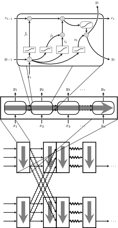
Figure 4: A hierarchical illustration of a deep X-LSTM model with three layers and one cross-connection in the second layer. Left: A single LSTM block; all intermediate results, as described in Equations 14–19 ($i_{t}$, $j_{t}$, $f_{t}$ and $o_{t}$) are clearly marked. Middle: Replicating the LSTM cell to create an LSTM layer (for processing a given input sequence $\vec{x}$). Right: A cross-modal deep LSTM model with two streams of three layers, taking sequences of length 3. In the second layer, the hidden sequences are shared between the two streams by being passed through a separate LSTM layer and feature-wise concatenated with the main stream hidden sequence.

Figure 5: The three types of cross-connection strategies, and the three types of weight sharing strategies. Each arrow is an LSTM layer, dashed lines indicate the identity transformation, and all arrows going into the same node are concatenated. Connections between lines in the bottom row represent recurrent weight sharing. Top, left-to-right: X-LSTM (A), X-LSTM (B), X-LSTM (N). Bottom, left-to-right: SH-LSTM (ALL), SH-LSTM (WSL), SH-LSTM (CUT).

A.5 Weight objective success classification

We performed stratified 10-fold crossvalidation on the baseline classifiers as well as the proposed LSTM model. Given the bias of the obtained data towards failure (there being twice as many sequences labelled unsuccessful), and the fact that it is not generally obvious what the classification threshold for this task should be (it likely involves several tradeoffs), we use ROC curves (and the associated area under them) as our primary evaluation metric. For completeness, we also report the accuracy, precision, recall, F₁ score and the Matthews Correlation Coefficient [12] under the classification threshold which maximises the F₁ score.

Afterwards we sought to construct competitive X-LSTMs, and therefore we computed the AUCs of the individual unimodal LSTMs on a validation dataset, obtaining AUCs of $80.62\%$ (for weight), $80.17\%$ (for sleep) and $74.18\%$ (for steps). As anticipated, this was not far enough in order to reliably generate non-uniform X-LSTMs, so we proceeded to perform a grid search on the parameter $k$. We’ve originally taken steps of $5$, but as we found the differences between adjacent steps to be negligible, we report the AUC results for $k\in\{10,20,30\}$. The X-LSTM performed the best with $k=30$, and (B) cross-connections—we compare it directly with the LSTM, as well as the SH-LSTMs, and report its architecture in Table 2.

LSTM	X-LSTM (B, $k=30$)
76377 param.	75089 param.
21 features	wt: 15 features, sl: 12 features, st: 2 features
	wt $\rightsquigarrow$ sl: 9 features, wt $\rightsquigarrow$ st: 14 features
	sl $\rightsquigarrow$ wt: 6 features, sl $\rightsquigarrow$ st: 11 features
	st $\rightsquigarrow$ wt: 1 feature, st $\rightsquigarrow$ sl: 1 feature
42 features	wt: 29 features, sl: 24 features, st: 3 features
84 features	wt: 57 features, sl: 48 features, st: 5 features
Fully connected, 128-D
Fully connected, 64-D
Fully connected, 1-D

Table 2: Architectures for the considered LSTM and cross-modal LSTM models. Cross-connections are highlighted.

To confirm that the advantages demonstrated by our methodology are statistically significant, we have performed paired $t$-testing on the metrics of individual cross-validation folds, choosing a significance threshold of $p<0.05$. We find that all of the observed advantages in ROC-AUC are indeed statistically significant—verifying simultaneously that the recurrent models are superior to other baseline approaches, that the X-LSTM has significantly improved on its LSTM baselines and that cross-connecting is statistically beneficial (given the weaker performance of X-LSTM (N) despite being able to compute the most features overall). The SH-LSTM performed the best in its (WSL) variant (which allowed for more features to be allocated to weight and sleep streams, at the expense of the steps stream) but was even then unable to outperform the baseline LSTM—highlighting once again its lack of ability to accurately specify relative importances between modalities, which is essential for this task. The results are summarised by Tables 3–4 and Figure 6.

Metric	SVM	RF	GHMM	DNN	LSTM	SH-LSTM	X-LSTM
Accuracy	67.65%	70.97%	66.31%	68.93%	79.12%	78.49%	80.30%
Precision	52.54%	56.05%	51.26%	53.80%	67.25%	65.31%	68.66%
Recall	81.02%	81.34%	82.32%	83.02%	79.30%	82.95%	81.62%
F1 score	63.71%	66.25%	63.11%	65.18%	72.69%	72.98%	74.37%
MCC	39.74%	44.75%	38.57%	42.63%	56.60%	56.80%	59.45%
ROC AUC	76.77%	79.97%	74.86%	78.54%	86.91%	86.63%	88.07%
$p$-value	$2\cdot 10^{-12}$	$6\cdot 10^{-10}$	$7\cdot 10^{-11}$	$2\cdot 10^{-11}$	$1\cdot 10^{-4}$	$4\cdot 10^{-5}$	—

Table 3: Comparative evaluation results of the baseline models against the LSTMs after 10-fold crossvalidation. Reported X-LSTM is the best-performing (B, $k=30$). Reported SH-LSTM is the best-performing (WSL). All metrics except the ROC AUC reported for the classification threshold that maximises the F₁ score. Reported $p$-values are for the X-LSTM vs. each baseline for the ROC-AUC metric.

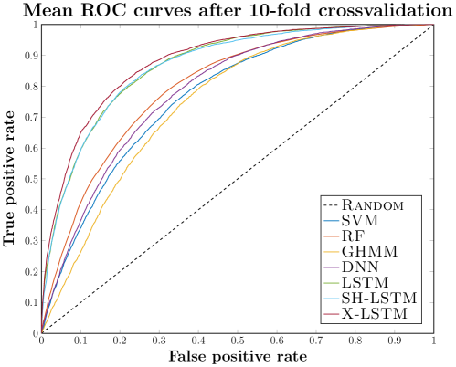
Figure 6: Mean ROC curves for the baselines, LSTM and the best-performing SH-LSTM and X-LSTM models.

Model	$k=10$	$k=20$	$k=30$
X-LSTM (A)	87.60%	87.60%	87.75%
X-LSTM (B)	87.21%	87.56%	88.07%
X-LSTM (N)	86.49%	86.98%	87.30%
$p$-value	$9.55\cdot 10^{-5}$	$0.021$	$1.03\cdot 10^{-3}$
SH-LSTM (ALL)	85.58%
SH-LSTM (WSL)	86.63%
SH-LSTM (CUT)	86.30%

Table 4: Effects of varying the hyperparameter $k$ and cross-connecting strategy of X-LSTMs to the mean ROC AUC after crossvalidation. Reported $p$-values are for the (N) vs. $\max$(A, B) strategies. We also report the mean ROC AUC for the three kinds of sharing strategies of SH-LSTMs.

A.6 Weight objective magnitude effects

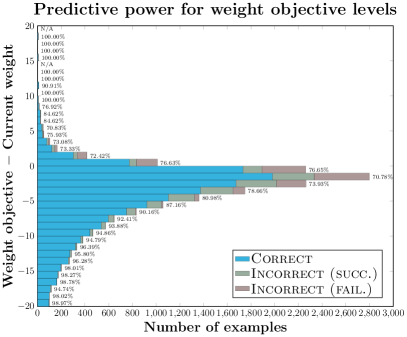
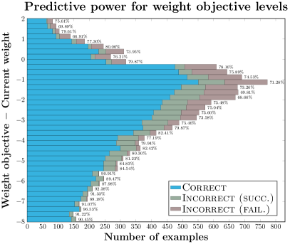
Figure 7: Left: A bar plot demonstrating the X-LSTM’s performance for different magnitudes of weight objectives (at the classification threshold of 0.5). Right: The same plot, zoomed in on the $[-8,2]$ range of weight objectives (where the majority of the examples are).

The magnitude of weight objectives set by users will have an obvious impact on the predictive power of the model. To illustrate this effect on the X-LSTM, we have aggregated its predictions across all of the crossvalidation folds (for a classification threshold of 0.5) into a histogram using bins of various weight objective magnitude ranges (ref. Figure 7). The histogram shows the proportion of correctly classified, incorrectly classified successful and incorrectly classified failed sequences.

The results closely match our expectations—at smaller weight objective magnitudes, the model is unbiased towards success or failure. However, starting at $-3\mathrm{kg}$ and moving higher, there is a clear bias towards misclassifying successful sequences, which eventually grows into nearly all misclassified sequences being successful. This kind of behaviour is fairly desirable—as it will encourage selection of realistic objectives, at the expense of making incorrect initial predictions about a few users that do eventually manage to achieve very ambitious goals.

References

- [1] Anton L. Beer, Tina Plank, and Mark W. Greenlee. Diffusion tensor imaging shows white matter tracts between human auditory and visual cortex. Experimental Brain Research, 213(2):299–308, 2011.
- [2] Cătălina Cangea, Petar Veličković, and Pietro Liò. XFlow: 1D-2D Cross-modal Deep Neural Networks for Audiovisual Classification. arXiv preprint arXiv:1709.00572, 2017.
- [3] Mark A Eckert, Nirav V Kamdar, Catherine E Chang, Christian F Beckmann, Michael D Greicius, and Vinod Menon. A cross-modal system linking primary auditory and visual cortices: Evidence from intrinsic fMRI connectivity analysis. Human brain mapping, 29(7):848–857, 2008.
- [4] Xavier Glorot and Yoshua Bengio. Understanding the difficulty of training deep feedforward neural networks. In International Conference on Artificial Intelligence and Statistics, pages 249–256, 2010.
- [5] Alex Graves. Generating sequences with recurrent neural networks. arXiv preprint arXiv:1308.0850, 2013.
- [6] Kaiming He, Xiangyu Zhang, Shaoqing Ren, and Jian Sun. Delving deep into rectifiers: Surpassing human-level performance on imagenet classification. In Proceedings of the IEEE International Conference on Computer Vision, pages 1026–1034, 2015.
- [7] Sepp Hochreiter and Jürgen Schmidhuber. Long short-term memory. Neural computation, 9(8):1735–1780, 1997.
- [8] Sergey Ioffe and Christian Szegedy. Batch normalization: Accelerating deep network training by reducing internal covariate shift. arXiv preprint arXiv:1502.03167, 2015.
- [9] Rafal Jozefowicz, Wojciech Zaremba, and Ilya Sutskever. An Empirical Exploration of Recurrent Network Architectures. In Proceedings of The 32nd International Conference on Machine Learning, pages 2342–2350, 2015.
- [10] Diederik Kingma and Jimmy Ba. Adam: A method for stochastic optimization. arXiv preprint arXiv:1412.6980, 2014.
- [11] C Kleiser, N Wawro, M Stelmach-Mardas, H Boeing, K Gedrich, H Himmerich, and J Linseisen. Are sleep duration, midpoint of sleep and sleep quality associated with dietary intake among Bavarian adults? European Journal of Clinical Nutrition, 2017.
- [12] Brian W Matthews. Comparison of the predicted and observed secondary structure of T4 phage lysozyme. Biochimica et Biophysica Acta (BBA)-Protein Structure, 405(2):442–451, 1975.
- [13] Vinod Nair and Geoffrey E Hinton. Rectified linear units improve restricted boltzmann machines. In Proceedings of the 27th International Conference on Machine Learning (ICML-10), pages 807–814, 2010.
- [14] Arlet V Nedeltcheva, Jennifer M Kilkus, Jacqueline Imperial, Kristen Kasza, Dale A Schoeller, and Plamen D Penev. Sleep curtailment is accompanied by increased intake of calories from snacks. The American journal of clinical nutrition, 89(1):126–133, 2009.
- [15] Jiquan Ngiam, Aditya Khosla, Mingyu Kim, Juhan Nam, Honglak Lee, and Andrew Y Ng. Multimodal deep learning. In Proceedings of the 28th international conference on machine learning (ICML-11), pages 689–696, 2011.
- [16] John C. Platt. Probabilistic Outputs for Support Vector Machines and Comparisons to Regularized Likelihood Methods. In ADVANCES IN LARGE MARGIN CLASSIFIERS, pages 61–74. MIT Press, 1999.
- [17] Jimmy Ren, Yongtao Hu, Yu-Wing Tai, Chuan Wang, Li Xu, Wenxiu Sun, and Qiong Yan. Look, Listen and Learn — a Multimodal LSTM for Speaker Identification. In Proceedings of the Thirtieth AAAI Conference on Artificial Intelligence, AAAI’16, pages 3581–3587. AAAI Press, 2016.
- [18] Natsuko Sato-Mito, Satoshi Sasaki, Kentaro Murakami, Hitomi Okubo, Yoshiko Takahashi, Shigenobu Shibata, Kazuhiko Yamada, Kazuto Sato, Freshmen in Dietetic Courses Study II Group, et al. The midpoint of sleep is associated with dietary intake and dietary behavior among young Japanese women. Sleep medicine, 12(3):289–294, 2011.
- [19] Karen Simonyan, Andrea Vedaldi, and Andrew Zisserman. Deep inside convolutional networks: Visualising image classification models and saliency maps. arXiv preprint arXiv:1312.6034, 2013.
- [20] Nitish Srivastava, Geoffrey E Hinton, Alex Krizhevsky, Ilya Sutskever, and Ruslan Salakhutdinov. Dropout: a simple way to prevent neural networks from overfitting. Journal of Machine Learning Research, 15(1):1929–1958, 2014.
- [21] Nitish Srivastava and Ruslan R Salakhutdinov. Multimodal learning with deep boltzmann machines. In Advances in neural information processing systems, pages 2222–2230, 2012.
- [22] Petar Veličković, Duo Wang, Nicholas D Lane, and Pietro Liò. X-CNN: Cross-modal Convolutional Neural Networks for Sparse Datasets. arXiv preprint arXiv:1610.00163, 2016.
- [23] Zhengzheng Xing, Jian Pei, and Eamonn Keogh. A brief survey on sequence classification. ACM SIGKDD Explorations Newsletter, 12(1):40–48, 2010.
- [24] Weiping Yang, Jingjing Yang, Yulin Gao, Xiaoyu Tang, Yanna Ren, Satoshi Takahashi, and Jinglong Wu. Effects of Sound Frequency on Audiovisual Integration: An Event-Related Potential Study. PLoS ONE, 10(9):1–15, 09 2015.
- [25] Wojciech Zaremba, Ilya Sutskever, and Oriol Vinyals. Recurrent neural network regularization. arXiv preprint arXiv:1409.2329, 2014.