Finite Synchrosqueezing Transform Based On The STFT

Abstract

The Finite STST Synchrosqueezing transform is a time-frequency analysis method that can decompose finite complex signals into time-varying oscillatory components. This representation is sparse and invertible, allowing recovery of the original signal. The STFT Synchrosqueezing transform on finite dimensional signals has the advantage of an efficient matrix representation. This article defines the finite STFT Synchrosqueezing transform and describes some properties of this transform. We compare the finite STFT and the finite STFT Synchrosqueezing transform by applying these transforms to a set of signals.

Index Terms—  Finite STFT, Instantaneous frequency, Finite STFT Synchrosqueezing transform, Oscillatory signals.

1 Introduction

Time-frequency decompositions [3] present time-frequency information about local frequency variations. Various time-frequency representations can be used to analyze a signal. The Short-Time Fourier transform (STFT), e.g., [13] is applied to extract time-frequency information of a signal within the time-frequency plane. The continuous wavelet transform (CWT) [4] provides a time-frequency representation of a signal with a time and frequency localization that is appropriate for many natural processes. The S-transform proposed by Stockwell et al. [23] is a time-frequency analysis technique that combines elements of the CWT and the STFT, and has been widely applied on seismic data processing and analysis of behavior of the signal [12]. All fore-mentioned transforms provide blurry information about the signal [4, 9]. In contrast, the Synchrosqueezing transform is a time frequency analysis that provides more accurate information about local frequency variations.

The Synchrosqueezing transform [24, 25, 26, 28] is a time frequency analysis that aims to characterize time-varying oscillatory signals efficiently. The transform is designed to analyze signals of the form:

$$x\left(t\right)=\sum_{k^{\prime}=1}^{K}A_{k^{\prime}}\left(t\right)e^{2\pi i\phi_{k^{\prime}}\left(t\right)},$$ (1)

where $A_{k^{\prime}}\left(t\right)$ and $\phi_{k^{\prime}}\left(t\right)$ are an amplitude function and a phase function, respectively. The signal $x$ consist of different layers of oscillation, each with instantaneous time-varying information. The Synchrosqueezing transform is a powerful tool for the analysis of a signal based on the notion of instantaneous frequency. Instantaneous frequency is a natural extension of the usual Fourier frequency that describes how quickly a signal oscillates locally at a given point in time or, more generally, how a quickly a number of components of the signal oscillate locally at a given point in time.

The Synchrosqueezing transform has a wide range of applications including geophysics [16], global climate [25], economics[15] and medicine [26, 30, 32]. These applications lead in a natural manner to the consideration of the Synchrosqueezing transform for a finite dimensional Hilbert space. Thakur and Wu in [25] use a Gabor based signal analysis method that they call the STFT Synchrosqueezing transform. In fact, they analyze continuous domain signals $f\in\mathcal{L}^{2}\left(\mathbb{C}\right)$ that consist of a superposition of a finite number of oscillatory components. Then they propose an algorithm to recover these instantaneous frequencies from a finite set of uniformly or non-uniformly spaced samples. They also prove that similar results hold for real valued signals where $e^{2\pi i\phi_{k^{\prime}}\left(t\right)}$ is replaced by $\cos\left(2\pi\phi_{k^{\prime}}\left(t\right)\right)$ in (1). This motivates us to focus on the oscillatory decomposion of finite-dimensional signals and define the STFT Synchrosqueezing transform for them.

The STFT Synchrosqueezing transform on finite groups can be studied in the realm of numerical linear algebra. In the other words, it is defined based on the STFT on finite groups. However, the STFT Synchrosqueezing transform is based on the continuous STFT transform. The finite STFT has a matrix representation which is more convenient to work rather than the continuous STFT. It provides matrix factorization and for this reason finite short time Fourier analysis is more popular in engineering rather than the STFT. Moreover, the STFT Synchrosqueezing transform on a finite cyclic group can be studied numerically in order to better understand properties of STFT Synchrosqueezing transform on the real line. Similarly to the STFT transform, the relationships between the STFT Synchrosqueezing transform on the real line, on the integers, and on cyclic groups can be studied based on a sampling and periodization argument [25, 28]. On the other hand, the delta function, which is used in the STFT Synchrosqueezing transform, can not be defined on $\mathcal{L}^{2}\left(\mathbb{C}\right)$ and an approximation delta is used instead of delta function. However, it is defined on $\mathbb{C}^{N}$.

In this paper, we consider that the continuous signal is sampled by $N$ regularly spaced samples. In other words, we assume $\phi_{k^{\prime}}$ and $A_{k^{\prime}}$ are naturally continuous functions but we are given only $\phi_{k^{\prime}}\left(n\right)$ and $A_{k^{\prime}}\left(n\right)$ for $n=0,\cdots,N-1$. As a result, we work with a periodic discrete function $x:\mathbb{Z}\rightarrow\mathbb{C}$ where $x\left(k+N\right)=x\left(k\right)$ for $k\in\mathbb{Z}$. It is of the form:

$$x\left(n\right)=\sum_{k^{\prime}=1}^{K}A_{k^{\prime}}\left(n\right)\mathrm{e}^{2\pi i\frac{\phi_{k^{\prime}}\left(n\right)}{N}},\quad n=0,1,\cdots,N-1.$$ (2)

This paper structured as follows. We start with a brief introduction of the STFT transform for finite dimensional signals and some of its properties in section II. In section III, we discuss the instantaneous frequency information and the finite Synchrosqueezing transform for finite, purely harmonic signals. Then, we demonstrate how to use the definition of instantaneous frequency information of pure harmonic signals to approximate the instantaneous frequency of an oscillatory signal. Then we define the finite Synchrosqueezing transform and show how we can extract the oscillatory components. In section IV we show that the results given in section III also are true for real signals where the exponentials $\mathrm{e}^{2\pi i\frac{\phi_{k^{\prime}}\left(n\right)}{N}}$ are replaced by $\cos\left(2\pi\frac{\phi_{k^{\prime}}\left(n\right)}{N}\right)$ in (2). In Section V, we show that the finite Synchrosqueezing transform has the stability property. Section VI is devoted to some comparative numerical results.

2 Preliminaries and Notations

To define the STFT-Synchrosqueezing transform for finite dimensional signals, we first recall the short time Fourier transform for finite dimensional signals. We index the components of a vector $x\in\mathbb{C}^{N}$ by $\{0,1,\cdots,N-1\}$, i.e., the cyclic group $\mathbb{Z}_{N}$. We will write $x\left(k\right)$ instead of $\mathbf{x}_{k}$ to avoid algebraic operations on indices.

The discrete Fourier transform is basic in short time Fourier analysis and is defined as

$$\mathcal{F}x\left(m\right)=\hat{x}\left(m\right)=\sum_{n=0}^{N-1}x\left(n\right)e^{-2\pi im\frac{n}{N}}.$$

The most important properties of the Fourier transform are the Fourier inversion formula and the Plancherel formula [1, 21, 22, 20]. The inversion formula shows that any $x$ can be written as a linear combination of harmonics. This means the normalized harmonics $\{\frac{1}{\sqrt{N}}e^{2\pi im\frac{\left(.\right)}{N}}\}_{m=0}^{N-1}$ form an orthonormal basis of $\mathbb{C}^{N}$ and hence we have

$$x=\frac{1}{N}\sum_{m=0}^{N-1}\hat{x}\left(m\right)e^{2\pi im\frac{\left(.\right)}{N}}\quad x\in\mathbb{C}^{N}.$$

Moreover, the Plancherel formula states

$$\langle x,y\rangle=\frac{1}{N}\langle\hat{x},\hat{y}\rangle\quad x,y\in\mathbb{C}^{N},$$

which results in

$$\sum_{n=0}^{N-1}|x\left(n\right)|^{2}=\frac{1}{N}\sum_{m=0}^{N-1}|\hat{x}\left(m\right)|^{2},$$

where $|x\left(n\right)|^{2}$ quantifies the energy of the signal $x$ at time $n$, and where the right-hand side indicates that the harmonic $e^{2\pi im\frac{\left(.\right)}{N}}$ contributes energy $\frac{1}{N}|\hat{x}\left(m\right)|^{2}$ to $x$.

Short time Fourier analysis is the interplay of the Fourier transform, translation operators, and modulation operators. The cyclic translation operator $T_{k}:\mathbb{C}^{N}\rightarrow\mathbb{C}^{N}$ is given by

$$T_{k} \mathbf{x}=T_{k}\left(x\left(0\right),\cdots,x\left(N-1\right)\right)^{t}$$

$$=\left(x\left(N-k\right),x\left(N-k+1\right),x\left(0\right),\cdots,x\left(N-k-1\right)\right)^{t}.$$

It is seen that the operator $T_{k}$ alters the position of the entries of $x$ and that, equivalently, $n-k$ is achieved modulo $N$.

Similarly, the modulation operator $M_{l}:\mathbf{C}^{N}\rightarrow\mathbb{C}^{N}$ is given by

$$M_{l} x=\left(e^{-2\pi il\frac{0}{N}}x\left(0\right),\right.$$

$$\left.e^{-2\pi il\frac{1}{N}}x\left(1\right),\cdots,e^{-2\pi il\frac{N-1}{N}}x\left(N-1\right)\right)^{t}.$$

The modulation operators are implemented as the pointwise product of the vector with harmonics $e^{-2\pi il\frac{.}{N}}$.

The translation and modulation operators are time-shift and frequency-shift operators, respectively. The time-frequency shift operator $\pi\left(k,l\right)$ is the combination of translation operators and modulation operators:

$$\pi\left(k,l\right):\mathbb{C}^{N}\rightarrow\mathbb{C}^{N}\quad\pi\left(k,l\right)x=M_{l}T_{k}x.$$

Hence, the STFT $V_{g}:\mathbb{C}^{N}\rightarrow\mathbb{C}^{N\times N}$ with respect to the window $g\in\mathbb{C}^{N}$ for every $x\in\mathbb{C}^{N}$ can be written as

$$V_{\phi}x\left(k,l\right)=\langle x,\pi\left(k,l\right)\phi\rangle=\sum_{n=0}^{N-1}x\left(n\right)\overline{g\left(n-k\right)}e^{-2\pi il\frac{n}{N}},$$

where $\overline{g}$ is the conjugate of $g$. The STFT uses a window function $g$, supported at a neighborhood of zero that is translated by $k$. Hence, the pointwise product with $\mathbf{x}$ selects a portion of $\mathbf{x}$ centered in time at $k$, and this portion is analyzed using a Fourier transform.

3 Finite Synchrosqueezing Transform of Harmonic Signal

In this section, we show how we can estimate the instantaneous frequency information based on short time Fourier transform. We first motivate the idea of finding instantaneous freuency information by considering the instantaneous frequency of a purely harmonic signal,

$$x\left(n\right)=Ae^{\frac{2\pi i\omega n}{N}}.$$ (3)

That is, we first define the instantaneous frequency information for a purely harmonic signals. Then we extend this definition to a combination of elementary oscillations. To introduce an instantaneous frequency information formula, we define the modified STFT:

$$V_{g} x\left(n,l\right)=\langle x,T_{n}M_{l}g\rangle=\sum_{k=0}^{N-1}x\left(k\right)\overline{g\left(k-n\right)}e^{-2\pi il\frac{k-n}{N}}$$

$$=e^{2\pi il\frac{n}{N}}\sum_{k=0}^{N-1}x\left(k\right)\overline{g\left(k-n\right)}e^{-2\pi il\frac{k}{N}}.$$

Consider a smooth window function $g$ is given. By Plancherel’s theorem, we can write $V_{g}x$, the short time Fourier transform of $x$ of (3) with respect to $g$ as

$$V_{g}x\left(n,l\right) =\langle x,T_{n}M_{l}g\rangle=\frac{1}{N}\langle\hat{x},M_{-n}T_{l}\hat{g}\rangle$$

$$=\frac{1}{N}\sum_{\xi=0}^{N-1}\hat{x}\left(\xi\right)\overline{T_{l}\hat{g}\left(\xi\right)}e^{\frac{2\pi in\xi}{N}}$$

$$=\frac{A}{N}\sum_{\xi=0}^{N-1}\delta\left(\xi-\omega\right)\overline{\hat{g}\left(\xi-l\right)}e^{\frac{2\pi in\xi}{N}}$$

$$=\frac{A}{N}\hat{g}\left(\omega-l\right)e^{\frac{2\pi in\omega}{N}}.$$

Motivated by the above analysis, we now define for a signal $x$ of the form (3), for any $\left(n,l\right)$ where $V_{g}x\left(n,l\right)\neq 0$, the instantaneous frequency information $\omega_{x}\left(n,l\right)$ as

$$\omega_{x}\left(n,l\right)=\mathrm{round}\left(\frac{1}{\frac{2\pi i}{N}}\mathrm{ln}\left(\frac{V_{g}x\left(n+1,l\right)}{V_{g}x\left(n,l\right)}\right)\right).$$ (4)

It should be noted that the instantaneous frequency information must be an integer for the defininition of the STFT Synchrosqueezing transform. However, $\omega$ is not necessary integer. This is the reason why we need the rounding function to find the nearest integer number to the instantaneous frequency. The rounding function used in (4) is given by

$$\mathrm{round}\left(x\right)=\left\{\begin{array}[]{ll}\left[x\right]&x\leq\left[x\right]+0.5\\ \left[x+1\right]&x>\left[x\right]+0.5\end{array}\right.$$

where $\left[x\right]$ is the integer part of $x$.

Note that the instantantaneous frequency information, in general, does not need to be equal to the instantaneous frequency of a given signal. In the context of the STFT Synchrosqueezing transform this implies that $\omega_{x}(n,l)$, in general, differs from the frequency $l$. In fact, as will be shown below, the transform “squeezes” energy to the frequency $l$ that equals the instaneous frequency information $\omega_{x}(n,l)$.

We now are ready to define the STFT Synchrosqueezing based on the phase function for $x$ of the form (3):

$$S_{\phi}x\left(n,\xi\right)=\sum_{l=0}^{N-1}V_{\phi}x\left(n,l\right)\delta\left(\xi-\omega_{x}\left(n,l\right)\right).$$

Thus, the Synchrosqueezing transform squeezes the energy in the frequency direction to the instantaneous frequency information of the purely harmonic signal.

Next, based on the definition of instantaneous frequency information of purely harmonic signals and the STFT Synchrosqueezing transform, we generalize these notions for oscillatory signals with multiple components. To this purpose, we define a function class of functions with well-separated oscillatory components:

Definition 1.

The space $\mathcal{A}_{d}\subset\mathbb{C}^{N}$ of superpositions consist of functions $x$ having the form

$$x\left(n\right)=\sum_{k^{\prime}=1}^{K}x_{k^{\prime}}\left(n\right),$$

for some $K>0$ and $x_{k^{\prime}}\left(n\right)=A_{k^{\prime}}\left(n\right)e^{\frac{2\pi\phi_{k^{\prime}}\left(n\right)}{N}}$ and $\phi_{k^{\prime}}$ satisfy

$$\phi^{\prime}_{k^{\prime}}\left(n\right)-\phi^{\prime}_{k^{\prime}+1}\left(n\right)>d\quad\textrm{for every\,\,}n\in\mathbb{Z}_{N},$$

where $d\leq N-1$

Functions in $\mathcal{A}_{d}$ are composed of a summation of oscillatory components and the instantaneous frequencies of any two consecutive components are separated by at least $d$. For a given window function $g\in\mathbb{C}^{N}$, we can apply the modified short time Fourier transform to any $x\in\mathcal{A}_{d}$. Similarly, we can define the instantaneous frequency information as:

Definition 2 (Instantaneous frequency information function).

Let $x\in\mathcal{A}_{d}$. Select a window function $\phi\in\mathbb{C}^{N}$ such that $|\mathrm{supp}\left(\hat{g}\right)|<\frac{d}{2}$. The instantaneous frequency information $\omega_{x}\left(k,l\right)$ is defined by

$$\omega_{x}\left(n,l\right)=\left\{\begin{array}[]{ll}\mathrm{round}\left(\mathrm{real}\left(\frac{1}{\frac{2\pi i}{N}}\mathrm{ln}\left(\frac{V_{g}x\left(n+1,l\right)}{V_{g}x\left(n,l\right)}\right)\right)\right)&V_{g}x\left(n,l\right)\neq 0\\ 0&V_{g}x\left(n,l\right)=0\end{array}\right.$$ (5)

We define the finite Synchrosqueezing transform based on the instantaneous frequency information as follows:

Definition 3.

Let $x\in\mathcal{A}_{d}$. Select a window function $g\in\mathbb{C}^{N}$ such that $|\mathrm{supp}\left(\hat{g}\right)|<\frac{d}{2}$. The STFT Synchrosqueezing transform is defined by

$$S_{g}x\left(n,\xi\right)=\sum_{l=0}^{N-1}V_{g}x\left(n,l\right)\delta\left(\xi-\omega_{x}\left(n,l\right)\right).$$

The following theorem states that the error between instantaneous frequency $\phi^{\prime}_{k_{0}}$ and instantaneous frequency information $\omega_{x}\left(n,l\right)$ is less than a given $\epsilon$. Before we provide the Theorem, we define some notations:

$$I_{s}^{1}=\sum_{k=0}^{N-1}|g\left(k-n\right)||k-n|^{s}$$

and

$$I_{s}^{2}=\sum_{k=0}^{N-1}|g\left(k-n-1\right)||k-n|^{s}.$$

Moreover, we denote $Z_{k^{\prime}}=\{\left(n,l\right):|l-\phi_{k^{\prime}}\left(n\right)|<\frac{d}{2}\}$ for each $k^{\prime}\in\{1,\cdots,K\}$.

We can now state the main theorem with related to the finite STFT Synchrosqueezing transform:

Theorem 3.1.

Consider a signal $x\in\mathcal{A}_{d}$ is given. Select a window function $g\in\mathbb{C}^{N}$ such that $|\mathrm{supp}\left(\hat{g}\right)|<\frac{d}{2}$. Moreover consider $\|\phi^{\prime\prime}_{k^{\prime}}\|_{\infty}\leq\epsilon\|\phi^{\prime}_{k^{\prime}}\|_{\infty}$ and $\|A^{\prime}_{k^{\prime}}\|_{\infty}\leq\epsilon\|\phi^{\prime}_{k^{\prime}}\|_{\infty}$. Also, let $\delta=\min\{V_{g}x\left(n,l\right);0\leq n,l\leq N-1,V_{g}x\left(n,l\right)\neq 0\}$ and $M=\max\{1,\frac{V_{g}x\left(n,l\right)}{V_{g}x\left(n+1,l\right)}\}$. Then, we have the following

$$\begin{split}&|\omega_{x}\left(n,l\right)-\phi^{\prime}_{k_{0}}\left(n\right)|\\ &\leq\frac{NM\epsilon}{2\pi\delta}\left[\sum_{k^{\prime}=1}^{K}\|\phi^{\prime}_{k^{\prime}}\|_{\infty}\left(I_{1}^{1}+\pi|A_{k^{\prime}}\left(n\right)|I_{2}^{1}+I_{1}^{2}+\pi|A_{k^{\prime}}\left(n\right)|I_{2}^{2}\right)\right]\\ &\quad+0.5=\tilde{\epsilon}\end{split}$$ (6)

where $\left(n,l\right)\in Z_{k_{0}}$.

Furthermore, if $\left(n,l\right)\notin Z_{k^{\prime}}$ for every $k^{\prime}=1,\cdots,K$, then

$$|V_{g}x\left(n,l\right)|\leq\sum_{k^{\prime}=0}^{K}\epsilon\|\phi^{\prime}_{k^{\prime}}\|_{\infty}\left(I_{1}^{1}+\pi|A_{k^{\prime}}\left(n\right)|I_{2}^{1}\right).$$ (7)

and

$$|V_{g}x\left(n+1,l\right)|\leq\sum_{k^{\prime}=0}^{K}\epsilon\|\phi^{\prime}_{k^{\prime}}\|_{\infty}\left(I_{1}^{2}+\pi|A_{k^{\prime}}\left(n\right)|I_{2}^{2}\right).$$ (8)

Theorem 3.1 basically tells us how to recover instantaneous frequencies for multi-component oscillatory signals. It shows that the error of instantaneous frequencies obtained from the formula (5) is less than $\tilde{\epsilon}$. Next we prove the theorem.

Proof.

To prove the inequality (6) we have

$$|\omega_{x}\left(n,l\right)-{\phi^{\prime}}_{k_{0}}\left(n\right)|$$

$$=\left|\mathrm{round}\left(\mathrm{real}\left(\frac{N}{2\pi i}\mathrm{ln}\left(\frac{V_{g}x\left(n+1,l\right)}{V_{g}x\left(n,l\right)}\right)\right)\right)-\phi^{\prime}_{k_{0}}\left(n\right)\right|$$

$$\leq\left|\frac{N}{2\pi i}\mathrm{ln}\left(\frac{V_{g}x\left(n+1,l\right)}{V_{g}x\left(n,l\right)}\right)-\phi^{\prime}_{k_{0}}\left(n\right)\right|+0.5$$

$$=\frac{N}{2\pi}\left|\mathrm{ln}\left(\frac{V_{g}x\left(n+1,l\right)}{V_{g}x\left(n,l\right)}\right)-\mathrm{ln}e^{\frac{2\pi i\phi^{\prime}_{k_{0}}\left(n\right)}{N}}\right|+0.5$$

$$\leq\frac{N}{2\pi}M\left|\frac{V_{g}x\left(n+1,l\right)}{V_{g}x\left(n,l\right)}-e^{\frac{2\pi i\phi^{\prime}_{k_{0}}\left(n\right)}{N}}\right|+0.5$$ (9)

$$\leq\frac{N}{2\pi}M$$

$$\left[\left|\frac{V_{g}x\left(n+1,l\right)-e^{\frac{2\pi i\phi^{\prime}_{k_{0}}\left(n\right)}{N}}A_{k_{0}}\left(n\right)e^{\frac{2\pi i\phi_{k_{0}}\left(n\right)}{N}}\hat{g}\left(l-\phi^{\prime}_{k_{0}}\left(n\right)\right)}{V_{g}x\left(n,l\right)}\right|\right.$$

$$\left.+\left|e^{\frac{2\pi i\phi^{\prime}_{k_{0}}\left(n\right)}{N}}\frac{A_{k_{0}}\left(n\right)e^{\frac{2\pi i\phi_{k_{0}}\left(n\right)}{N}}\hat{g}\left(l-\phi^{\prime}_{k_{0}}\left(n\right)\right)-V_{g}x\left(n,l\right)}{V_{g}x\left(n,l\right)}\right|\right]$$

$$+0.5$$ (10)

We derived (9) by the mean value theorm.

Note that $A_{k_{0}}\left(n\right)e^{\frac{2\pi i\phi_{k_{0}}\left(n\right)}{N}}\hat{g}\left(l-\phi^{\prime}_{k_{0}}\left(n\right)\right)=0$ for $\left(n,l\right)\notin Z_{k^{\prime}}$ for any $k^{\prime}=1,\cdots,K$, since $|\mathrm{supp}\left(\hat{g}\right)|<\frac{d}{2}$. Hence we can rewrite the second part of (10) as:

$$| A_{k_{0}}\left(n\right)e^{\frac{2\pi i\phi_{k_{0}}\left(n\right)}{N}}\hat{g}\left(l-\phi^{\prime}_{k_{0}}\left(n\right)\right)-V_{g}x\left(n,l\right)|$$

$$=|\sum_{k^{\prime}=1}^{K}\left(A_{k^{\prime}}\left(n\right)e^{\frac{2\pi i\phi_{k^{\prime}}\left(n\right)}{N}}\sum_{k=0}^{N-1}g\left(k-n\right)e^{\frac{-2\pi i}{N}\left(l-\phi^{\prime}_{k^{\prime}}\left(n\right)\right)\left(k-n\right)}\right.$$

$$\left.-\sum_{k=0}^{N-1}A_{k^{\prime}}\left(k\right)e^{\frac{2\pi i\phi_{k^{\prime}}\left(k\right)}{N}}g\left(k-n\right)e^{\frac{-2\pi il\left(k-n\right)l}{N}}\right)|$$

$$\leq\sum_{k^{\prime}=1}^{K}\left(\sum_{k=0}^{N-1}|A_{k^{\prime}}\left(k\right)-A_{k^{\prime}}\left(n\right)||g\left(k-n\right)|\right.$$

$$\left.+\sum_{k=0}^{N-1}|A_{k^{\prime}}\left(n\right)g\left(k-n\right)||e^{\frac{2\pi i\phi_{k^{\prime}}\left(k\right)}{N}}-e^{\frac{2\pi i}{N}\left[\phi_{k^{\prime}}\left(n\right)+\phi^{\prime}_{k^{\prime}}\left(n\right)\left(k-n\right)\right]}|\right)$$

$$\leq\sum_{k^{\prime}=1}^{K}\left(\|A_{k^{\prime}}^{\prime}\|_{\infty}\sum_{k=0}^{N-1}|g\left(k-n\right)||k-n|\right.$$

$$\left.+|A_{k^{\prime}}\left(n\right)|\sum_{k=0}^{N-1}|g\left(k-n\right)|\pi\|\phi^{\prime\prime}_{k^{\prime}}\|_{\infty}|k-n|^{2}\right)$$ (11)

$$\leq\sum_{k^{\prime}=0}^{K}\epsilon\|\phi^{\prime}_{k^{\prime}}\|_{\infty}\left(I_{1}^{1}+\pi|A_{k^{\prime}}\left(n\right)|I_{2}^{1}\right).$$ (12)

We can derive (11) using a Taylor expansion:

$$|1-e^{\frac{2\pi i}{N}\left[-\phi_{k^{\prime}}\left(k\right)+\phi_{k^{\prime}}\left(n\right)+\phi^{\prime}_{k^{\prime}}\left(n\right)\left(k-n\right)\right]}|$$

$$\leq\pi\|{\phi^{\prime\prime}}_{k^{\prime}}\|_{\infty}|k-n|^{2}.$$

The first part of inequality (10) can be written as:

$$| V_{g}x\left(n+1,l\right)-e^{\frac{2\pi i}{N}\left(\phi^{\prime}_{k_{0}}\left(n\right)\right)}A_{k_{0}}\left(n\right)e^{\frac{2\pi i\phi_{k_{0}}\left(n\right)}{N}}\hat{g}\left(l-\phi^{\prime}_{k_{0}}\left(n\right)\right)|.$$

$$=|\sum_{k^{\prime}=1}^{K}\left(\sum_{k=0}^{N-1}A_{k^{\prime}}\left(k\right)e^{\frac{2\pi i\phi_{k^{\prime}}\left(k\right)}{N}}g\left(k-n-1\right)e^{\frac{-2\pi il\left(k-n-1\right)}{N}}\right.$$

$$\left.-\sum_{k=0}^{N-1}A_{k^{\prime}}\left(n\right)g\left(k-n-1\right)e^{\frac{-2\pi i}{N}\left(l-\phi^{\prime}_{k^{\prime}}\left(n\right)\right)\left(k-n-1\right)}\right.$$

$$\left.e^{\frac{2\pi i{\phi^{\prime}}_{k^{\prime}}\left(n\right)}{N}}e^{\frac{2\pi i\phi_{k^{\prime}}\left(n\right)}{N}}\right)|$$

$$\leq\sum_{k^{\prime}=1}^{K}\sum_{k=0}^{N-1}|g\left(k-n-1\right)|$$

$$|A_{k^{\prime}}\left(k\right)e^{\frac{2\pi i\phi_{k^{\prime}}\left(k\right)}{N}}-A_{k^{\prime}}\left(n\right)e^{\frac{2\pi i}{N}\left[\phi\left(n\right)+\phi^{\prime}_{k^{\prime}}\left(n\right)\left(k-n\right)\right]}|$$

$$\leq\sum_{k^{\prime}=1}^{K}\sum_{k=0}^{N-1}|g\left(k-n-1\right)|\left[|A_{k^{\prime}}\left(k\right)\right.$$

$$\left.-A_{k^{\prime}}\left(n\right)|+|A_{k^{\prime}}\left(n\right)||e^{\frac{2\pi i\phi_{k^{\prime}}\left(k\right)}{N}}-e^{\frac{2\pi i}{N}\left[\phi_{k^{\prime}}\left(n\right)+\phi^{\prime}_{k^{\prime}}\left(n\right)\left(k-n\right)\right]}|\right]$$

$$\leq\sum_{k^{\prime}=1}^{K}\left(\|A_{k^{\prime}}^{\prime}\|_{\infty}\sum_{k=0}^{N-1}|g\left(k-n-1\right)||k-n|\right.$$

$$\left.+|A_{k^{\prime}}\left(n\right)|\sum_{k=0}^{N-1}|g\left(k-n-1\right)|\pi\|\phi^{\prime\prime}_{k^{\prime}}\|_{\infty}|k-n|^{2}\right)$$

$$\leq\sum_{k^{\prime}=0}^{K}\epsilon\|\phi^{\prime}_{k^{\prime}}\|_{\infty}\left(I_{1}^{2}+\pi|A_{k^{\prime}}\left(n\right)|I_{2}^{2}\right).$$ (13)

By considering the inequalities (10), (12) and (13) we have

$$|\omega_{x}\left(n,l\right)-\phi^{\prime}_{k_{0}}\left(n\right)|\leq$$

$$\frac{NM\epsilon}{2\pi\delta}\left[\sum_{k^{\prime}=1}^{K}\|\phi^{\prime}_{k^{\prime}}\|_{\infty}\left(I_{1}^{1}+\pi|A_{k^{\prime}}\left(n\right)|I_{2}^{1}+I_{1}^{2}+\pi|A_{k^{\prime}}\left(n\right)|I_{2}^{2}\right)\right]+0.5=\tilde{\epsilon}.$$

Now by the fact that $A_{k_{0}}\left(n\right)e^{\frac{2\pi i\phi_{k_{0}}\left(n\right)}{N}}\hat{g}\left(l-{\phi^{\prime}}_{k_{0}}\left(n\right)\right)=0$ for $\left(n,l\right)\notin Z_{k^{\prime}}$ and by (12) and (13) we can derive the inequalities (7) and (8). ∎

For an appropriate signal $x\in\mathbb{C}^{N}$, the energy in the Synchrosqueezing transform $S_{g}x\left(n,\xi\right)$ is concentrated around the instantaneous frequency curves $\{\phi^{\prime}_{k^{\prime}}\left(n\right)\}$. Once $S_{g}x$ is computed, we can recover each of the components by completing the invertion of the STFT and take the summation over small bands around each instantaneous frequency curve.

Theorem 3.2.

Consider a signal $x\in\mathcal{A}_{d}$ and a window function $g\in\mathbb{C}^{N}$ are given such that $|\mathrm{supp}\left(\hat{g}\right)|<\frac{d}{2}$. Moreover, assume $\|\phi^{\prime\prime}_{k^{\prime}}\|_{\infty}\leq\epsilon\|\phi^{\prime}_{k^{\prime}}\|_{\infty}$ and $\|A^{\prime}_{k^{\prime}}\|_{\infty}\leq\epsilon\|\phi^{\prime}_{k^{\prime}}\|_{\infty}$. Let $\delta=\min\{V_{g}x\left(n,l\right);0\leq n,l\leq N-1,V_{g}x\left(n,l\right)\neq 0\}$ and $M=\max\{1,\frac{V_{g}x\left(n,l\right)}{V_{g}x\left(n+1,l\right)}\}$. Then for each $n=0,1,\cdots,N-1$ and $k^{\prime}\in\{1,2,\cdots,K\}$ we have

$$A_{k^{\prime}}\left(n\right)e^{\frac{2\pi i}{N}\phi_{k^{\prime}}\left(n\right)}=\sum_{|\xi-\phi^{\prime}_{k^{\prime}}\left(n\right)|\leq\epsilon}S_{g}x\left(n,\xi\right)$$

Proof.

we have

$$\begin{split}&\sum_{|\xi-\phi^{\prime}_{k^{\prime}}\left(n\right)|\leq\epsilon}S_{g}x\left(n,\xi\right)\\ &=\sum_{|\xi-\phi^{\prime}_{k^{\prime}}\left(n\right)|\leq\tilde{\epsilon}}\sum_{l=0}^{N-1}V_{g}x\left(n,l\right)\delta\left(\xi-\omega_{x}\left(n,l\right)\right)\\ &=\sum_{l=0}^{N-1}V_{g}x\left(n,l\right)\sum_{|\xi-\phi^{\prime}_{k^{\prime}}\left(n\right)|\leq\tilde{\epsilon}}\delta\left(\xi-\omega_{x}\left(n,l\right)\right)\\ &=\sum_{\{l;|\omega_{x}\left(n,l\right)-\phi^{\prime}_{k^{\prime}}\left(n\right)|\leq\tilde{\epsilon}\}}V_{g}x\left(n,l\right)\end{split}$$ (14)

Now we obtain

$$\frac{1}{\overline{g}\left(0\right)}\sum_{|\xi-\phi^{\prime}_{k^{\prime}}\left(n\right)|\leq\tilde{\epsilon}}S_{g}x\left(n,\xi\right)$$

$$=\frac{1}{\overline{g}\left(0\right)}\sum_{\{l;|l-\phi^{\prime}_{k^{\prime}}\left(n\right)|\leq\frac{d}{4}\}}V_{g}x\left(n,l\right)$$

$$=\frac{1}{\overline{g}\left(0\right)}A_{k^{\prime}}\left(n\right)e^{\frac{2\pi i}{N}\phi_{k^{\prime}}\left(n\right)}\sum_{\{l;|l-\phi^{\prime}_{k^{\prime}}\left(n\right)|\leq\frac{d}{4}\}}\hat{g}\left(l-\phi^{\prime}_{k^{\prime}}\left(n\right)\right)$$

$$=A_{k^{\prime}}\left(n\right)e^{\frac{2\pi i}{N}\phi_{k^{\prime}}\left(n\right)}$$

∎

4 Finite Synchrosqueezing Transform of Real Signals

In this section we show that results similar to those in section 3 hold true for the real valued signal $x$, where the exponentials $e^{2\pi i\frac{\phi_{k^{\prime}}\left(n\right)}{N}}$ are replaced by $\cos\left(2\pi\frac{\phi_{k^{\prime}}\left(n\right)}{N}\right)$ in (2). Hence we define the function space $\mathcal{B}_{d}$ as all $x\in\mathcal{A}_{d}$ such that $e^{2\pi i\frac{\phi_{k^{\prime}}\left(n\right)}{N}}$ are replaced by $\cos\left(2\pi\frac{\phi_{k^{\prime}}\left(n\right)}{N}\right)$ in the definition 1.

In section 4 we proved that the error of instantaneous frequencies obtained from(5) for a signal $x\in\mathcal{A}_{d}$ is less than a given $\tilde{\epsilon}$. Now we show a similar result for $x\in\mathcal{B}_{d}$.

Theorem 4.1.

Consider a signal $x\in\mathcal{B}_{d}$ is given. Select a window function $g\in\mathbb{C}^{N}$ such that $|\mathrm{supp}\left(\hat{g}\right)|<\frac{d}{2}$. Moreover consider $\|\phi^{\prime\prime}_{k^{\prime}}\|_{\infty}\leq\epsilon\|\phi^{\prime}_{k^{\prime}}\|_{\infty}$ and $\|A^{\prime}_{k^{\prime}}\|_{\infty}\leq\epsilon\|\phi^{\prime}_{k^{\prime}}\|_{\infty}$. Also, let $\delta=\min\{V_{g}x\left(n,l\right);0\leq n,l\leq N-1,V_{g}x\left(n,l\right)\neq 0\}$ and $M=\max\{1,\frac{V_{g}x\left(n,l\right)}{V_{g}x\left(n+1,l\right)}\}$. Then, for any $\left(n,l\right)\in Z_{k_{0}}$ we have the following:

$$| \omega_{x}\left(n,l\right)-\phi^{\prime}_{k_{0}}\left(n\right)|$$

$$\leq\frac{NM\epsilon}{2\pi\delta}\left[\sum_{k^{\prime}=1}^{K}\|{\phi^{\prime}}_{k^{\prime}}\|_{\infty}\left(I_{1}^{1}+\pi|A_{k^{\prime}}\left(n\right)|I_{2}^{1}+I_{3}^{1}\right.\right.$$

$$\left.\left.+I_{1}^{2}+\pi|A_{k^{\prime}}\left(n\right)|I_{2}^{2}+I_{3}^{2}\right)\right]+0.5=\tilde{\epsilon},$$

where $I_{i}^{j}$ for $i,j=1,2$ is denoted the same as in the section $3$ and $I_{3}^{j}$ for $j=1,2$ is denoted as

$$I_{3}^{j}=\sum_{k=0}^{N-1}|g\left(k-n-j+1\right)||k+1|.$$

Furthermore, if $\left(n,l\right)\notin Z_{k^{\prime}}$ for every $k^{\prime}=1,\cdots,K$, then

$$|V_{g}x\left(n,l\right)|\leq\sum_{k^{\prime}=0}^{K}\epsilon\|\phi^{\prime}_{k^{\prime}}\|_{\infty}\left(I_{1}^{1}+\pi|A_{k^{\prime}}\left(n\right)|I_{2}^{1}+I_{3}^{1}\right).$$ (15)

and

$$|V_{g}x\left(n+1,l\right)|\leq\sum_{k^{\prime}=0}^{K}\epsilon\|\phi^{\prime}_{k^{\prime}}\|_{\infty}\left(I_{1}^{2}+\pi|A_{k^{\prime}}\left(n\right)|I_{2}^{2}+I_{3}^{2}\right).$$ (16)

Proof.

Similar to the proof of Theorem 3.1 we have

$$|\omega_{x}\left(n,l\right)-{\phi^{\prime}}_{k_{0}}\left(n\right)|$$

$$=\left|\mathrm{round}\left(\mathrm{real}\left(\frac{N}{2\pi i}\mathrm{ln}\left(\frac{V_{g}x\left(n+1,l\right)}{V_{g}x\left(n,l\right)}\right)\right)\right)-\phi^{\prime}_{k_{0}}\left(n\right)\right|\leq\frac{N}{2\pi}M$$

$$\left[\left|\frac{V_{g}x\left(n+1,l\right)-e^{\frac{2\pi i\phi^{\prime}_{k_{0}}\left(n\right)}{N}}A_{k_{0}}\left(n\right)e^{\frac{2\pi i\phi_{k_{0}}\left(n\right)}{N}}\hat{g}\left(l-\phi^{\prime}_{k_{0}}\left(n\right)\right)}{V_{g}x\left(n,l\right)}\right|\right.$$

$$\left.+\left|e^{\frac{2\pi i\phi^{\prime}_{k_{0}}\left(n\right)}{N}}\frac{A_{k_{0}}\left(n\right)e^{\frac{2\pi i\phi_{k_{0}}\left(n\right)}{N}}\hat{g}\left(l-\phi^{\prime}_{k_{0}}\left(n\right)\right)-V_{g}x\left(n,l\right)}{V_{g}x\left(n,l\right)}\right|\right]$$

$$+0.5$$ (17)

Now considering $A_{k_{0}}\left(n\right)e^{\frac{2\pi i\phi_{k_{0}}\left(n\right)}{N}}\hat{g}\left(l-\phi^{\prime}_{k_{0}}\left(n\right)\right)=0$ for $\left(n,l\right)\notin Z_{k^{\prime}}$ for any $k^{\prime}=1,\cdots,K$, since $|\mathrm{supp}\left(\hat{g}\right)|<\frac{d}{2}$, we can rewrite the second part of the last inequality of (17) as:

$$| A_{k_{0}}\left(n\right)e^{\frac{2\pi i\phi_{k_{0}}\left(n\right)}{N}}\hat{g}\left(l-\phi^{\prime}_{k_{0}}\left(n\right)\right)-V_{g}x\left(n,l\right)|$$

$$=|\sum_{k^{\prime}=1}^{K}\left(A_{k^{\prime}}\left(n\right)e^{\frac{2\pi i\phi_{k^{\prime}}\left(n\right)}{N}}\sum_{k=0}^{N-1}g\left(k-n\right)e^{\frac{-2\pi i}{N}\left(l-\phi^{\prime}_{k^{\prime}}\left(n\right)\right)\left(k-n\right)}\right.$$

$$\left.-\sum_{k=0}^{N-1}A_{k^{\prime}}\left(k\right)\cos\left(\frac{2\pi\phi_{k^{\prime}}\left(k\right)}{N}\right)\left(k-n\right)e{\frac{-2i\pi l\left(k-n\right)l}{N}}\right)|$$

$$\leq\sum_{k^{\prime}=1}^{K}\left(|A_{k^{\prime}}\left(n\right)e^{\frac{2\pi i\phi_{k^{\prime}}\left(n\right)}{N}}\sum_{k=0}^{N-1}g\left(k-n\right)e^{\frac{-2\pi i}{N}\left(l-\phi^{\prime}_{k^{\prime}}\left(n\right)\right)\left(k-n\right)}\right.$$

$$\left.-\sum_{k=0}^{N-1}A_{k^{\prime}}\left(k\right)e^{\frac{2\pi i\phi_{k^{\prime}}\left(k\right)}{N}}g\left(k-n\right)e{\frac{-2i\pi l\left(k-n\right)l}{N}}|\right.$$

$$\left.+|\sum_{k=0}^{N-1}A_{k^{\prime}}\left(k\right)\sin\left(\frac{2\pi\phi_{k^{\prime}}g\left(k\right)}{N}\right)\left(k-n\right)e{\frac{-2i\pi l\left(k-n\right)l}{N}}|\right).$$ (18)

By the fact that $A_{k^{\prime}}$ is naturally a continous function and without a loss of generality we can assume $A_{k^{\prime}}\left(-1\right)=0$. As a result, by the mean value theorem and by the inequality (12) we can rewrite the second part of (18) as

$$| A_{k_{0}}\left(n\right)e^{\frac{2\pi i\phi_{k_{0}}\left(n\right)}{N}}\hat{g}\left(l-\phi^{\prime}_{k_{0}}\left(n\right)\right)-V_{g}x\left(n,l\right)|$$

$$\leq\sum_{k^{\prime}=0}^{K}\epsilon\|{\phi^{\prime}}_{k^{\prime}}\|_{\infty}\left(I_{1}^{1}+\pi|A_{k^{\prime}}\left(n\right)|I_{2}^{1}\right)$$

$$+|\sum_{k=0}^{N-1}A_{k^{\prime}}\left(k\right)-A_{k^{\prime}}\left(-1\right)\sin\left(\frac{2\pi\phi_{k^{\prime}}\left(k\right)}{N}\right)g\left(k-n\right)|$$

$$\leq\sum_{k^{\prime}=0}^{K}\left(\epsilon\|\phi^{\prime}_{k^{\prime}}\|_{\infty}\left(I_{1}^{1}+\pi|A_{k^{\prime}}\left(n\right)|I_{2}^{1}\right)\right.$$

$$\left.+|\sum_{k=0}^{N-1}\|{A^{\prime}}_{k^{\prime}}\|_{\infty}|k+1|+g\left(k-n\right)|\right)$$

$$\leq\sum_{k^{\prime}=0}^{K}\left(\epsilon\|\phi^{\prime}_{k^{\prime}}\|_{\infty}\left(I_{1}^{1}+\pi|A_{k^{\prime}}\left(n\right)|I_{2}^{1}\right)\right.$$

$$\left.+|\sum_{k=0}^{N-1}\epsilon\|{\phi^{\prime}}_{k^{\prime}}\|_{\infty}|k+1|+g\left(k-n\right)|\right)$$

$$\leq\sum_{k^{\prime}=0}^{K}\epsilon\|\phi^{\prime}_{k^{\prime}}\|_{\infty}\left(I_{1}^{1}+\pi|A_{k^{\prime}}\left(n\right)|I_{2}^{1}+I_{3}^{1}\right).$$ (19)

Similarly to the procedure of (19) and based on the inequality (13) we can write the first part of (17) as

$$|V_{g}x \left(n+1,l\right)-e^{\frac{2\pi i}{N}\left(\phi^{\prime}_{k_{0}}\left(n\right)\right)}A_{k_{0}}\left(n\right)e^{\frac{2\pi i\phi_{k_{0}}\left(n\right)}{N}}\hat{g}\left(l-\phi^{\prime}_{k_{0}}\left(n\right)\right)|.$$

$$\leq\sum_{k^{\prime}=0}^{K}\epsilon\|\phi^{\prime}_{k^{\prime}}\|_{\infty}\left(I_{1}^{2}+\pi|A_{k^{\prime}}\left(n\right)|I_{2}^{2}+I_{3}^{2}\right).$$ (20)

By inequalities (17), (19) and (20) we have

$$|\omega_{x}\left(n,l\right)-\phi^{\prime}_{k_{0}}\left(n\right)|$$

$$\leq\frac{NM\epsilon}{2\pi\delta}\left[\sum_{k^{\prime}=1}^{K}\|\phi^{\prime}_{k^{\prime}}\|_{\infty}\left(I_{1}^{1}+\pi|A_{k^{\prime}}\left(n\right)|I_{2}^{1}+I_{3}^{1}\right.\right.$$

$$\left.\left.+I_{1}^{2}+\pi|A_{k^{\prime}}\left(n\right)|I_{2}^{2}+I_{3}^{2}\right)\right]+0.5=\tilde{\epsilon}.$$

We can derive the inequalities (15) and (16) using the same procedure as usin for the proof of Theorem 3.1. ∎

Now by the same argument that was used for the proof of Theorem 3.2 we have:

Theorem 4.2.

Consider a signal $x\in\mathcal{B}_{d}$ is given. Select a window function $g\in\mathbb{C}^{N}$ such that $|\mathrm{supp}\left(\hat{g}\right)|<\frac{d}{2}$. Moreover consider $\|\phi^{\prime\prime}_{k^{\prime}}\|_{\infty}\leq\epsilon\|\phi^{\prime}_{k^{\prime}}\|_{\infty}$ and $\|A^{\prime}_{k^{\prime}}\|_{\infty}\leq\epsilon\|\phi^{\prime}_{k^{\prime}}\|_{\infty}$. Let $\delta=\min\{V_{g}x\left(n,l\right);0\leq n,l\leq N-1,V_{g}x\left(n,l\right)\neq 0\}$ and $M=\max\{1,\frac{V_{g}x\left(n,l\right)}{V_{g}x\left(n+1,l\right)}\}$. Then we have

$$A_{k^{\prime}}\left(n\right)\cos\left(\frac{2\pi}{N}\phi_{k^{\prime}}\left(n\right)\right)=\sum_{|\xi-\phi^{\prime}_{k^{\prime}}\left(n\right)|\leq\epsilon}S_{g}x\left(n,\xi\right),$$

for all $n=0,1,\cdots,N-1$ and all $k^{\prime}\in\{1,2,\cdots,K\}$.

5 Consistency and Stability of Finite Synchrosqueezing Transform

In this section we show that the finite Synchrosqueezing transform has a stability property similar to that shown for the continuous transform (shown in [24]). To this purpose we present a theorem that shows the error of the instantaneous frequency information obtained by formula (5) for noisy signal is less than an $\tilde{\epsilon}$ which is given in the Theorem.

Theorem 5.1.

Consider a signal $x\in\mathcal{B}_{d}$ is given. Select a window function $g\in\mathbb{C}^{N}$ such that $|\mathrm{supp}\left(\hat{g}\right)|<\frac{d}{2}$. Moreover consider $\|\phi^{\prime\prime}_{k^{\prime}}\|_{\infty}\leq\epsilon\|\phi^{\prime}_{k^{\prime}}\|_{\infty}$ and $\|A^{\prime}_{k^{\prime}}\|_{\infty}\leq\epsilon\|\phi^{\prime}_{k^{\prime}}\|_{\infty}$. Also, let $\delta=\min\{V_{g}x\left(n,l\right);0\leq n,l\leq N-1,V_{g}x\left(n,l\right)\neq 0\}$ and $M=\max\{1,\frac{V_{g}x\left(n,l\right)}{V_{g}x\left(n+1,l\right)}\}$.

Furthermore, suppose we have a noisy signal $e\in\mathbb{C}^{N}$ such that $\|e\|_{\infty}\|g\|_{1}\leq\epsilon^{\prime}$. Letting $y=x+e$, the following statements holds for each $k^{\prime}$ and $\left(n,l\right)\in Z_{k^{\prime}}$

$$| \omega_{y}\left(n,l\right)-\phi^{\prime}_{k_{0}}\left(n\right)|$$

$$\leq\frac{NM\epsilon}{2\pi\delta}\left[\sum_{k^{\prime}=1}^{K}\|\phi^{\prime}_{k^{\prime}}\|_{\infty}\left(I_{1}^{1}+\pi|A_{k^{\prime}}\left(n\right)|I_{2}^{1}+I_{3}^{1}\right.\right.$$

$$\left.\left.+I_{1}^{2}+\pi|A_{k^{\prime}}\left(n\right)|I_{2}^{2}+I_{3}^{2}\right)\right]+0.5+\frac{N{M^{\prime}}{\epsilon^{\prime}}}{\pi}$$

$$=\tilde{\epsilon}+\frac{NM^{\prime}\epsilon^{\prime}}{\pi},$$

where $I_{i}^{j}$ for $i,j=1,2$ is denoted the same as in the section $3$ and $I_{3}^{j}$ for $j=1,2$ is denoted as

$$I_{3}^{j}=\sum_{k=0}^{N-1}|g\left(k-n-j+1\right)||k+1|.$$

Furthermore, if $\left(n,l\right)\notin Z_{k^{\prime}}$ for every $k^{\prime}=1,\cdots,K$, then

$$|V_{g}y\left(n,l\right)|\leq\sum_{k^{\prime}=0}^{K}\epsilon\|\phi^{\prime}_{k^{\prime}}\|_{\infty}\left(I_{1}^{1}+\pi|A_{k^{\prime}}\left(n\right)|I_{2}^{1}+I_{3}^{1}\right)+\frac{NM^{\prime}\epsilon^{\prime}}{\pi}.$$ (21)

and

$$|V_{g}y\left(n+1,l\right)|\leq\sum_{k^{\prime}=0}^{K}\epsilon\|\phi^{\prime}_{k^{\prime}}\|_{\infty}\left(I_{1}^{2}+\pi|A_{k^{\prime}}\left(n\right)|I_{2}^{2}+I_{3}^{2}\right)+\frac{NM^{\prime}\epsilon^{\prime}}{\pi}.$$ (22)

Proof.

By considering the assumptions, we have

$$|\omega_{y}\left(n,l\right)-{\phi^{\prime}}_{k^{\prime}}\left(n\right)|$$

$$\leq|\omega_{y}\left(n,l\right)-\tilde{\omega}_{x}\left(n,l\right)|+|\tilde{\omega}_{x}\left(n,l\right)-{\phi^{\prime}}_{k^{\prime}}\left(n\right)|,$$

where $\tilde{\omega}_{x}\left(n,l\right)$ is the instantaneous frequency information of $x$ at the point $\left(n,l\right)$ without rounding. From Theorem (4.1) we have

$$|\omega_{x}\left(n,l\right)-\phi^{\prime}_{k_{0}}\left(n\right)|$$

$$\leq\frac{NM\epsilon}{2\pi\delta}\left[\sum_{k^{\prime}=1}^{K}\|\phi^{\prime}_{k^{\prime}}\|_{\infty}\left(I_{1}^{1}+\pi|A_{k^{\prime}}\left(n\right)|I_{2}^{1}+I_{3}^{1}\right.\right.$$

$$\left.\left.+I_{1}^{2}+\pi|A_{k^{\prime}}\left(n\right)|I_{2}^{2}+I_{3}^{2}\right)\right]=\tilde{\epsilon}-0.5.$$ (23)

On the other hand

$$|\omega_{y}\left(n,l\right)-\omega_{x}\left(n,l\right)|$$

$$=|\mathrm{round}\left(\mathrm{real}\left(\frac{N}{2\pi i}\ln\frac{V_{g}y\left(n+1,l\right)}{V_{g}y\left(n,l\right)}\right)\right)$$

$$\quad-\mathrm{real}\left(\ln\frac{V_{g}x\left(n+1,l\right)}{V_{g}x\left(n,l\right)}\right)|$$

$$\leq\frac{N}{2\pi}|\ln\frac{V_{g}y\left(n+1,l\right)}{V_{g}y\left(n,l\right)}-\ln\frac{V_{g}x\left(n+1,l\right)}{V_{g}x\left(n,l\right)}|+0.5$$

$$\leq\frac{NM^{\prime}}{2\pi}|V_{g}y\left(n+1,l\right)-V_{g}y\left(n,l\right)$$

$$\quad-V_{g}x\left(n+1,l\right)+V_{g}x\left(n,l\right)|+0.5$$

$$\leq\frac{NM^{\prime}}{2\pi}\left(|V_{g}y\left(n+1,l\right)-V_{g}x\left(n+1,l\right)|\right.$$

$$\left.\quad+|V_{g}y\left(n,l\right)-V_{g}x\left(n,l\right)|\right)+0.5$$

$$\leq\frac{NM^{\prime}}{2\pi}\left(|\sum_{k=0}^{N-1}e\left(k\right)g\left(k-n-1\right)e^{\frac{-2\pi ikl}{N}}|\right.$$

$$\left.\quad+|\sum_{k=0}^{N-1}e\left(k\right)g\left(k-n\right)e^{\frac{-2\pi ikl}{N}}|\right)+0.5$$

$$\leq\frac{NM^{\prime}}{2\pi}\left(2\|e\|_{\infty}\|g\|_{1}\right)+0.5$$

$$\leq\frac{NM^{\prime}\epsilon^{\prime}}{\pi}+0.5.$$ (24)

By the inequalities (23) and (24) we have

$$|\omega_{y}\left(n,l\right)-\phi^{\prime}_{k_{0}}\left(n\right)|\leq\frac{NM^{\prime}\epsilon^{\prime}}{\pi}+\tilde{\epsilon}.$$

Furthermore, the inequalities (21) and (22) follow from (24) and (15) and (16). ∎

In the following theorem we will show how to reconstruct an oscillation from a noisy signal.

Theorem 5.2.

Consider a signal $x\in\mathcal{B}_{d}$ is given. Pick a window function $g\in\mathbb{C}^{N}$ such that $|\mathrm{supp}\left(\hat{g}\right)|<\frac{d}{2}$. Moreover consider $\|\phi^{\prime\prime}_{k^{\prime}}\|_{\infty}\leq\epsilon\|\phi^{\prime}_{k^{\prime}}\|_{\infty}$ and $\|A^{\prime}_{k^{\prime}}\|_{\infty}\leq\epsilon\|\phi^{\prime}_{k^{\prime}}\|_{\infty}$. Also, let $\delta=\min\{V_{g}x\left(n,l\right);0\leq n,l\leq N-1,V_{g}x\left(n,l\right)\neq 0\}$ and $M=\max\{1,\frac{V_{g}x\left(n,l\right)}{V_{g}x\left(n+1,l\right)}\}$.

Furthermore, suppose we have a noisy signal $e\in\mathbb{C}^{N}$ such that $\|e\|_{\infty}\|g\|_{1}\leq\epsilon^{\prime}$. For $y=x+e$, we have

$$|A_{k^{\prime}}\left(n\right)\cos\left(\frac{2\pi}{N}\phi_{k^{\prime}}\left(n\right)\right)-\sum_{|\xi-\phi^{\prime}_{k^{\prime}}\left(n\right)|\leq\epsilon}S_{g}y\left(n,\xi\right)|\leq\epsilon^{\prime},$$

for all $n=0,1,\cdots,N-1$ and all $k^{\prime}\in\{1,2,\cdots,K\}$.

Proof.

From (14) we have

$$|A_{k^{\prime}}\left(n\right)\cos\left(\frac{2\pi}{N}\phi_{k^{\prime}}\left(n\right)\right)-\sum_{|\xi-\phi^{\prime}_{k^{\prime}}\left(n\right)|\leq\epsilon}S_{g}y\left(n,\xi\right)|$$

$$\leq|A_{k^{\prime}}\left(n\right)\cos\left(\frac{2\pi}{N}\phi_{k^{\prime}}\left(n\right)\right)-\sum_{\{l;|\omega_{x}\left(n,l\right)-\phi^{\prime}_{k^{\prime}}\left(n\right)|\leq\tilde{\epsilon}\}}V_{g}y\left(n,l\right)|$$

$$\leq|A_{k^{\prime}}\left(n\right)\cos\left(\frac{2\pi}{N}\phi_{k^{\prime}}\left(n\right)\right)$$

$$-\sum_{\{l;|\omega_{x}\left(n,l\right)-\phi^{\prime}_{k^{\prime}}\left(n\right)|\leq\tilde{\epsilon}\}}V_{g}x\left(n,l\right)+V_{g}e\left(n,l\right)|.$$

Now by the Theorem 4.2 we have

$$|A_{k^{\prime}}\left(n\right)\cos \left(\frac{2\pi\phi_{k^{\prime}}\left(n\right)}{N}\right)$$

$$-\sum_{\{l|\omega_{x}\left(n,l\right)-\phi^{\prime}_{k^{\prime}}\left(n\right)|\leq\tilde{\epsilon}\}}V_{g}x\left(n,l\right)+V_{g}e\left(n,l\right)|$$

$$\leq|\sum_{\{l|\omega_{x}\left(n,l\right)-\phi^{\prime}_{k^{\prime}}\left(n\right)|\leq\tilde{\epsilon}\}}V_{g}e\left(n,l\right)|$$

$$\leq|\sum_{k=0}^{N-1}e\left(k\right)g\left(k-n\right)e^{\frac{-2\pi ikl}{N}}|$$

$$\leq\sum_{k=0}^{N-1}|e\left(k\right)g\left(k-n\right)e^{\frac{-2\pi ikl}{N}}|$$

$$\leq\|e\|_{\infty}\sum_{k=0}^{N-1}|g\left(k-n\right)|$$

$$\leq\epsilon^{\prime}.$$

∎

6 Numerical Results

In this section, we apply the algorithms of sections 3 and 4 for several test cases. We consider a chirp signal, a multi-component signal and a signal with interlacing instantaneous frequency elements and these signals with noise. We compute the instantaneous frequency of these signals using the finite STFT Synchrosqueezing transform. For the instantaneous-frequency computation, we use a window function such that its Fourier transform is a Hann function with a support of $10$ samples.

To evaluate the performance of finite STFT Synchrosqueezing transform, we compare the time varying power spectrum of the finite STFT Synchrosqueezing transform and the finite STFT transform with the ideal time-varying power spectrum(itvPS) of the test signals. We define the itvPS of the signal of the form (2) as:

$$P_{x}\left(n,\xi\right)=\sum_{k^{\prime}=1}^{K}A_{k^{\prime}}\left(n\right)^{2}\delta\left(\xi-\phi^{\prime}_{k^{\prime}}\left(n\right)\right).$$ (25)

The first signal is a single-component chirp signal

$$x\left(n\right)=\cos\left(2\pi\left(\frac{n}{20}+0.05\left(\frac{n}{20}\right)^{2}\right)\right),$$ (26)

for $n=0,\cdots,199$. The phase function of (26) is equal to

$$\phi\left(n\right)=10n+\frac{1}{40}n^{2},$$

and the instantaneous frequency is

$${\phi}^{\prime}\left(n\right)=10+\frac{1}{20}n.$$ (27)

The finite STFT and the finite STFT Synchrosqueezing transform of (26) are shown in Figure 1.

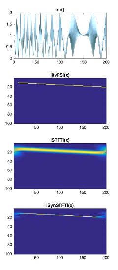
Fig. 1: Top: The chirp signal (26) First middle: The itvPS of the signal $x$ Second middle: The finite STFT of the signal$x$. Bottom: The finite STFT Synchrosqueezing transform of the signal $x$.

It is seen from Figure 1 that the finite STFT Synchrosqueezing transform has a better estimation of the instantaneous frequency given in (27).

The second signal is a two-component signal that is given by

$$x\left(n\right)=\cos\left(2\pi\left(\frac{n}{10}+0.2\left(\frac{n}{10}\cos\left(\frac{n}{10}\right)\right)\right)\right)$$ (28)

$$+\cos\left(2\pi\left(\frac{3n}{10}+0.02\left(\frac{n}{10}\right)^{2}\right)\right),$$

for $n=0,\cdots,199$. The phase functions of the signal (28) are equal to

$$\phi_{1}\left(n\right)=40n+4\cos\left(\frac{n}{10}\right),$$

and

$$\phi_{2}\left(n\right)=60n+\frac{4}{100}n^{2}.$$

Consequently, the instantaneous frequencies are equal to

$$\phi^{\prime}_{1}\left(n\right)=40-\frac{4}{10}\sin\left(\frac{n}{10}\right),$$ (29)

and

$$\phi^{\prime}_{2}\left(n\right)=60+\frac{8}{100}n.$$ (30)

The finite STFT and the finite STFT Synchrosqueezing transform of (28) are shown in Figure 2. Note that the support of the window function in the frequency domain is $10$ samples which is less than the separation of the two consequative instantaneous frequencies, which is 20 samples.

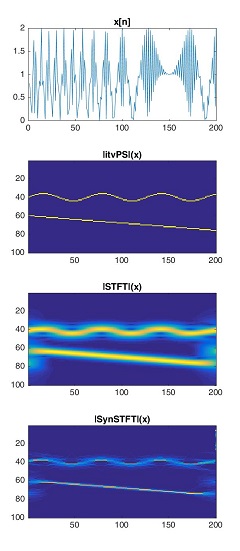
Fig. 2: Top: The two component signal (28) . First middle: The itvPS of the signal $x$. Second middle: The finite STFT of the signal$x$. Bottom: The finite STFT Synchrosqueezing transform of the signal $x$.

Figure 2 shows that the energy in the finite STFT Synchrosqueezing transform is better concentrated around the instantaneous frequencies (29) and (30) as compared to the finite STFT.

The third signal is a signal with interlacing frequency elements

$$x\left(n\right)=\cos\left(5\pi\left(\frac{n}{10}\right)\right)+\cos\left(2\pi\left(\frac{n}{10}+0.05\left(\frac{n}{10}\right)^{2}\right)\right),$$ (31)

for $n=0,\cdots,199$. The phase functions of the signal (31) are equal to

$$\phi_{1}\left(n\right)=50n,$$

and

$$\phi_{2}\left(n\right)=20n+\frac{1}{10}n^{2},$$

which results in the instantaneous frequencies

$$\phi^{\prime}_{1}\left(n\right)=50,$$

and

$$\phi^{\prime}_{2}\left(n\right)=20+\frac{1}{5}n.$$

The finite STFT and the finite STFT Synchrosqueezing transform of (31) are shown in Figure 3. Although the signal in Figure 3 is not in $\mathcal{B}_{d}$, the result is well separated.

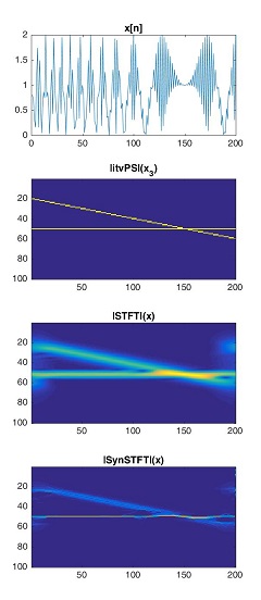
Fig. 3: Top: The signal with interlacing frequency elements (31) First middle: The itvPS of the signal $x$. Second middle: The finite STFT of the signal$x$. Bottom: Finite STFT Synchrosqueezing transform of the signal $x$.

We also added some noise to these three signals before applying the finite STFT Synchrosqueezing transform and finite STFT transform. The results are shown in figures 4, 5 and 6. It is seen that the finite STFT Synchrosqueezing transform is more robust to noise than finite STFT transform.

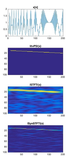
Fig. 4: Top: The noisy signal $y=x+e$ where $\|e\|_{\infty}=0.4$ and $x$ as defined in (26). First middle: The itvPS of the signal $y$. Second middle: The finite STFT of the noisy signal $y$. Bottom: Finite STFT Synchrosqueezing transform of the noisy signal $y$.

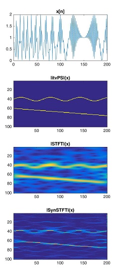
Fig. 5: Top: The noisy signal $y=x+e$ where $\|e\|_{\infty}=0.4$ and $x$ as defined in (28). First middle: The itvPS of the signal $y$. Second middle: The finite STFT of the noisy signal $y$. Botton: The finite STFT Synchrosqueezing transform of the noisy signal $y$.

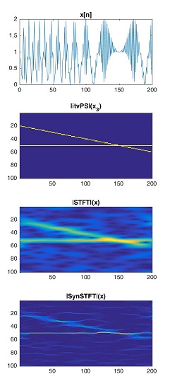
Fig. 6: Top: The noisy signal $y=x+e$ where $\|e\|_{\infty}=0.4$ and $x$ as defined in (31). First middle: The itvPS of the signal $y$. Second middle: The finite STFT of the noisy signal $y$. Botton: The finite STFT Synchrosqueezing transform of the noisy signal $y$.

References

• [1] M.J. Bastiaans, M. Geilen, On the discrete Gabor transform and the discrete Zak transform. Signal Process. 49(3), 151-166 (1996).
• [2] T. Berkant and J. L. Patrick, Comments on the Interpretation of Instantaneous Frequency, IEEE Sig. Proc. Letters, 4 (1997), pp. 123–125.
• [3] L. Cohen, Time-frequency distributions—Review, Proc. IEEE, vol. 77, no. 7, pp. 941-981, Jul. 1989.
• [4] I. Daubechies, Ten Lectures on Wavelets, Society for Industrial and Applied Mathematics, 1992.
• [5] I. Daubechies, S. Maes, A nonlinear squeezing of the continuous wavelet transform based on auditory nerve models, in Wavelets in Medicine and Biology ed. by A. Aldroubi, M. Unser(CRC Press, Boca Raton, 1996), pp. 527-546.
• [6] I. Daubechies, J. Lu, H.-T. Wu, Synchrosqueezed wavelet transforms: an empirical mode decomposition-like tool. Appl. Comput. Harmon. Anal. 30(2), 243-261 (2011).
• [7] R. J. Duffin and A. C. Schaeffer. A Class of Nonharmonic Fourier Series. Trans. American Math. Soc., 72(2):341-366, 1952.
• [8] H.G. Feichtinger, K. Grchenig, Gabor frames and time-frequency analysis of distributions., J. Funct. Anal. 146(2), 464-495 (1996).
• [9] P. Flandrin, Time-Frequency/Time-Scale Analysis. Wavelet Analysis and Its Applications,vol. 10 (Academic, San Diego, CA, 1999)
• [10] W. Fulton and J. Harris. Representation Theory: A First Course. Springer, New York, 1991.
• [11] D. Gabor, Theory of communication, J. Inst. Elect. Eng.—Part III: Radio Commun. Eng., vol. 93, no. 26, pp. 429-457, 1946
• [12] J. Gao, W. Chen, Y. Li, and F. Tian, Generalized S transform and seismic response analysis of thin interbeds, Chin. J. Geophys., vol. 46, no. 4, pp. 526-532, Jul. 2003.
• [13] K. Grochenig , Aspects of Gabor analysis on locally compact abelian groups, Gabor analysis and Algorithms, 211-231, Applied and Numerical Harmonic Analysis, Birkhauser, Boston, MA 1998.
• [14] K. Grochenig, Fundation of time-frequency analysis, Applied and Numerical Harmonic Analysis. Birkhauser, Boston, MA 1998.
• [15] S.K. Guharay, G.S. Thakur, F.J. Goodman, S.L. Rosen, D. Houser, Analysis of non-stationary dynamics in the financial system. Econ. Lett. 121, 454-457 (2013).
• [16] R.H. Herrera, J.-B. Tary, M. van der Baan, Time-frequency representation of microseismic signals using the Synchrosqueezing transform. GeoConvention (2013).
• [17] T. Hou, M. Yan, and Z. Wu. A variant of the emd method for multi-scale data. Advances in Adaptive Data Analysis, 1:483-516, 2009.
• [18] N. E. Huang, Z. Wu, S. R. Long, K. C. Arnold, K. Blank, and T. W. Liu. On instantaneous frequency. Advances in Adaptive Data Analysis, 1:177-229, 2009.
• [19] C. Li, M. Liang, A generalized Synchrosqueezing transform for enhancing signal time-frequency separation. Signal Process. 92, 2264-2274 (2012)
• [20] G. E. Pfander, Gabor frames in finite dimensions, in: Finite Frames, Appl. Numer. Harmon. Anal., Birkhäuser/Springer, New York, 2013, pp. 193-239 (Chapter VI).
• [21] S. Qiu, Discrete Gabor transforms: the Gabor-Gram matrix approach. J. Fourier Anal. Appl. 4 (1), 1-17 (1998).
• [22] S. Qiu, H. Feichtinger, Discrete Gabor structure and optimal representation. IEEE Trans. Signal Process. 43(10), 2258-2268 (1995).
• [23] R. Stockwell, L. Mansinha, and R. Lowe, Localization of the complex spectrum: The S transform, IEEE Trans. Signal Process., vol. 44, no. 4, pp. 998–1001, Apr. 1996.
• [24] G.Thakur, The Synchrosqueezing transform for instantaneous spectral analysis. In Excursions in harmonic analysis, vol. 4, 2014.
• [25] G. Thakur, H.-T. Wu, Synchrosqueezing-based recovery of instantaneous frequency from nonuniform samples. SIAM J. Math. Anal. 43(5), 2078-2095 (2011)
• [26] G. Thakur, E. Brevdo, N.-S. Fuckar, H.-T. Wu,The Synchrosqueezing algorithm for timevarying spectral analysis: robustness properties and new paleoclimate applications. Signal Process. 93, 1079-1094 (2013).
• [27] E. T. Whittaker and G. N. Watson, A Course of Modern Analysis, Fourth Ed., Cambridge Math. Library, Cambridge U. Press, Cambridge, UK, 1927.
• [28] H. T. Wu, Adaptive Analysis of Complex Data Sets., Thesis, 2012.
• [29] H.-T. Wu, Instantaneous frequency and wave shape functions. Appl. Comput. Harmon. Anal. 35, 181-199 (2013)
• [30] H.-T. Wu, Y.-H. Chan, Y.-T. Lin, Y.-H. Yeh, Using synchrosqueezing transform to discover breathing dynamics from ECG signals. Appl. Comput. Harmon. Anal. 36 (2), 354-359 (2014).
• [31] H.-T. Wu, P. Flandrin, and I. Daubechies. One or Two Frequencies? The Synchrosqueezing Answers. Adv. Adapt. Data Anal. 3 (01n02) (2011) 29-39.
• [32] H.-T. Wu, S.-S. Hseu, M.-Y. Bien, Y.R. Kou, I. Daubechies, Evaluating the physiological dynamics via Synchrosqueezing: Prediction of the Ventilator Weaning. IEEE Trans. Biomed. Eng. 61(3), 736-744 (2014).