Long Short-Term Memory for Japanese Word Segmentation

Abstract

This study presents a long short-term memory (LSTM) neural network approach to Japanese word segmentation (JWS). Previous studies on Chinese word segmentation have succeeded in using recurrent neural networks such as LSTM and gated recurrent units. However, in contrast to Chinese, Japanese includes several character types such as hiragana, katakana, and kanji, which produce orthographic variations and increase the difficulty of word segmentation. Additionally, while it is important to consider a global context, traditional JWS approaches still rely on local features. To address this problem, this study proposes employing an LSTM-based approach to JWS.

1 Introduction

Word segmentation is a fundamental task of Japanese language processing. Moreover, word segmentation errors in East Asian languages (e.g., Japanese and Chinese), which lack a trivial word segmentation process, can cause problems for downstream NLP applications. Thus, it is crucial to perform accurate word segmentation for the Japanese language.

To achieve high accuracy, modern Japanese word segmentation (JWS) methods utilize discriminative models relying on extensive feature engineering. However, machine-learning-based methods tend to require hand-crafted feature templates. Thus, they suffer from data sparseness. Neural network models have, therefore, been investigated for various NLP tasks to address the problem of feature engineering [Liu et al., 2015, Sutskever et al., 2014, Socher et al., 2013, Turian et al., 2010, Mikolov et al., 2013]. Neural network models enable the use of dense feature vectors (i.e., embeddings) that are learned via representation learning.

Another important problem in JWS corresponds to context modeling. Traditional JWS methods employ feature templates to expand local features in a fixed window. However, global information beyond the window is not considered. Conversely, recurrent neural network (RNN) models grasp long distance information owing to the use of long short–term memory (LSTM), achieving state-of-the-art accuracy in Chinese word segmentation [Chen et al., 2015b]. However, it is uncertain whether the LSTM approach is also effective for JWS because there are many types of character sets in Japanese that produce orthographic variations.

Therefore, we propose an LSTM network for JWS that incorporates character-level embeddings and long-distance dependency. The main contributions of this study are as follows.

• We propose an LSTM model for JWS and investigate methods to utilize sparse features, such as character type, character $n$-gram, and dictionary features.

• The experimental results indicate that the proposed word segmentation model achieves comparable performance to conventional approaches in both token- and sentence-level accuracy with respect to various datasets.

• Our souce code is available at GitHub.

2 LSTM for Japanese Word Segmentation

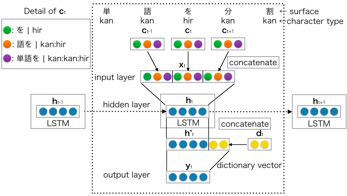
Figure 1: An overview of the proposed LSTM for JWS.

Machine-learning-based approaches for word segmentation build a classifier from an annotated corpus to classify the existence of word boundaries around a target character. In word segmentation, each character is assigned to several labels, such as {B, I, E, S}, {B, I, E}, and {B, I} to indicate the segmentation, where {B}, {I}, {E}, and {S} represents Begin, Inside, End, and Single, in that order. In JWS, the most prevalent label set corresponds to {B, I, E, S}, and the label sets do not significantly affect the accuracy of our preliminary experiments.

Classification of these labels is performed by running the Viterbi algorithm over a word lattice [Kudo et al., 2004, Nakagawa, 2004, Kaji and Kitsuregawa, 2013] or by independently performing predictions [Neubig et al., 2011]. However, previous approaches used feature templates to expand window-based local features. Thus, they suffered data sparseness and a lack of global information in a sentence. An RNN, such as LSTM, addresses the problem of the lack of history by using recurrent hidden units, in which the output at each time depends on that of the previous time. This method has been successfully demonstrated with respect to several NLP tasks, such as language modeling [Mikolov et al., 2010] and text generation [Sutskever et al., 2011].

Thus, we propose character-based embeddings and an LSTM network for JWS. Figure 1 shows an overview of the proposed framework. The model is similar to previous studies on CWS [Chen et al., 2015b] which uses character embeddings. However, our model also incorporates character-based $n$-gram embeddings (character $n$-gram and character type $n$-gram) and a word dictionary sparse feature in addition to character embeddings.

In the neural architecture, character-based embeddings for context characters are extracted via the lookup table layer and concatenated into a single vector, $\bm{x}_{t}\in\mathbb{R}^{H_{1}}$, where $H_{1}$ is the size of the input layer. Thereafter, $\bm{x}_{t}$ is passed into the next layer to perform the linear transformation, $\bm{W_{1}}$, followed by an element-wise activation function, $g$, such as sigmoid and $\tanh$ functions:

$$\bm{h}_{t}=g(\bm{W_{1}}\bm{x}_{t}+\bm{b_{1}})$$ (1)

where $\bm{W_{1}}\in\mathbb{R}^{H_{2}\times H_{1}}$, $\bm{b_{1}}\in\mathbb{R}^{H_{2}}$, and $\bm{h}_{t}\in\mathbb{R}^{H_{2}}$. Additionally, $H_{2}$ denotes a hyperparameter, which indicates the number of hidden units in the hidden layer. $\bm{b_{1}}$ denotes a bias vector, and $\bm{h}_{t}$ denotes the resulting hidden vector. The final output is obtained by running a softmax function after a similar linear transformation, $\bm{W_{2}}$, to the hidden vector as follows:

$$\bm{y}_{t}=\mathit{softmax}(\bm{W_{2}}\bm{h}_{t}+\bm{b_{2}})$$ (2)

where $\bm{W_{2}}$$\in$ $\mathbb{R}^{|T|\times H_{2}}$, $\bm{b_{2}}\in\mathbb{R}^{|T|}$, and $\bm{y}_{t}\in\mathbb{R}^{|T|}$. Thus, $\bm{b_{2}}$ denotes a bias vector, and $\bm{y}_{t}$ denotes the distribution vector for each possible label.

2.1 Character-Level Features

This section discusses character-level features, as shown in Figure 1. This paper introduces character embedding, character-type embedding, and their $n$-gram for JWS. We describe the character vector, $\bm{c}_{t}$, for JWS below. Formally, the character vector, $\bm{c}_{t}$, is defined as follows:

$$\bm{c}_{t}=\bm{l}_{t}\oplus\bm{e}_{t},$$ (3)

where $\oplus$ denotes concatenation of the vectors, and $\bm{l}_{t}$ and $\bm{e}_{t}$ denote character embeddings and character-type embeddings, respectively. These embeddings are fed to the input layer.

In the following subsections, we discuss three features frequently used in JWS, and we describe their realization as embeddings in the proposed architecture.

2.1.1 Character Embeddings

In a word segmentation task, a character dictionary, $C$, of size $|C|$ is often created. Traditional machine-learning approaches that use feature templates treat each character independently as a one-hot vector. However, it is natural for a neural network model to represent discrete data as distributed vectors or embeddings [Bengio et al., 2003, Collobert and Weston, 2008]. Representation learning is an actively studied topic in NLP because it overcomes the data sparseness problem. Thus, the same practice is followed to represent each character as a real-valued vector, $\bm{v_{c}}$ $\in$ $\mathbb{R}^{d}$, where $d$ is the dimensionality of the vector space. With respect to each character, the corresponding character embedding, $\bm{v_{c}}$, is selected by a lookup table.

2.1.2 Character-Type Embeddings

Character embeddings are extremely effective in identifying prefixes and postfixes. However, they can be too sparse when crossing a word boundary. To address this problem, it is helpful to exploit character types, such as hiragana, katakana, and kanji (e.g., ひらがな，カタカナ，漢字), for JWS [Neubig et al., 2011]. For example, katakana sequences tends to correspond to a loan word. A transition from a character type to another will likely correspond to a word boundary [Nagata, 1999].

2.1.3 Character-Based $n$-gram Embeddings

In addition to character type, the $n$-gram is effective in JWS [Neubig et al., 2011]. Thus, the character-type sequence information is incorporated as embeddings. Each character is converted to a one-hot vector corresponding to its character type. A one-hot vector comprises either hiragana, katakana, kanji, alphabet, number, symbol, start symbol, or terminal symbol. The advantages of a deep neural network include dealing with sparse vectors by converting them to dense vectors. This enables the utilization of a sparse feature, such as character trigram. Additionally, a character-based $n$-gram is effective for sentence similarity, part-of-speech tagging [Wieting et al., 2016], and for Japanese morphological analysis [Neubig et al., 2011]. Therefore, $n$-gram is used for character and character-type embeddings. More precisely, a one-hot vector is created for each unigram, bigram, and trigram. Each embedding is selected by a lookup table as well as unigram embeddings.

The embedding vectors $\bm{l}_{t}$ and $\bm{e}_{t}$ are defined as follows:

$$\bm{l}_{t} = \bm{l}_{[t-2:t]}\oplus\bm{l}_{[t-1:t]}\oplus\bm{l}_{[t]}$$ (4)

$$\bm{e}_{t} = \bm{e}_{[t-2:t]}\oplus\bm{e}_{[t-1:t]}\oplus\bm{e}_{[t]}$$ (5)

where $\bm{l}_{[a:b]}$ denotes the embedding for the strings from a to b. The same holds for $\bm{e}_{t}$.

2.2 Incorporating Word Dictionary

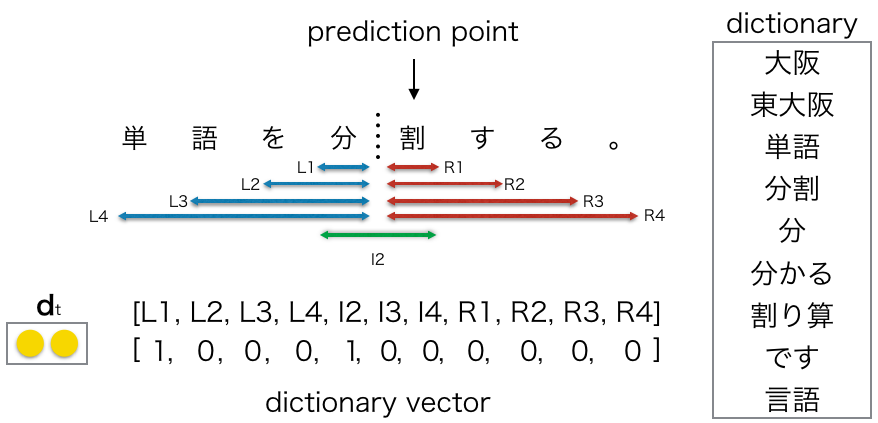
Figure 2: Example of a dictionary vector.

Character embeddings, character-type embeddings, and their $n$-gram extensions perform an excellent job with respect to learning character-based features from an annotated corpus. However, character-based JWS models lack word-level information useful in determining the character sequences constituting a word. Thus, a Japanese morphological analyzer typically uses a dictionary. It is essential for a JWS using a word lattice during decoding to use word-level information such as a unigram and a bigram. However, this is not necessary for character-based JWS approaches.

Notably, it is not trivial to encode dictionary information into a neural network architecture. ?) suggests that it is ineffective to learn both dense continuous and sparse discrete vector representations in the same layer. Thus, we follow the same practice to create a sparse dictionary vector. Whereas, instead of learning embeddings, this is used for the input to the final output layer, as shown in Figure 1.

Figure 2 illustrates the creation of a dictionary vector, comprising three parts, as follows: left-side feature $L$, right-side feature $R$, and inside-feature $I$. For example, L2 is activated if a word with a length corresponding to 2 exists in the dictionary on the left side of the prediction point. If the length of the word exceeds a certain threshold, the word length is cut off with respect to the length. In the study, 4 is adopted as the threshold, following ?). In contrast to $L$ and $R$, $I2$ is fired if there exists a word spanning the boundary and possesses a length of 2. It should be noted that $I$ is activated only if the length of the word exceeds 1, based on its definition. Finally, the feature vectors are concatenated to a single vector (e.g., a dictionary vector).

The dictionary vector, $\bm{d}_{t}$, is concatenated to the current hidden vector. It should be noted that the current hidden vector, $\bm{h}_{t}$, is on top of the LSTM network. Formally, the new hidden vector, $\bm{h^{\prime}}_{t}$, is defined as follows.

$$\bm{h^{\prime}}_{t}=\bm{h}_{t}\oplus\bm{d}_{t}.$$ (6)

2.3 Training

In this study, a cross-entropy error is adopted as a loss function. Given an output vector, $\bm{y}_{t}$, the loss in a correct distribution corresponding to $\bm{c}_{t}$ is computed as follows.

$$\bm{loss}=\sum_{t}-\bm{i}_{t}\log\bm{y}_{t}+\frac{1}{2}\lambda\|\theta\|_{2}^{2},$$ (7)

where $\bm{i}_{t}$ denotes the correct label distribution, $\lambda$ denotes a hyperparameter of L2 regularization, and $\theta$ indicates all parameters of the model.

Following [Socher et al., 2013], the diagonal variant of AdaGrad [Duchi et al., 2011] with mini batches is used to minimize the objective. The update for the $i$-th parameter, $\theta_{t,i}$, at time step $t$, is defined as follows.

$$\theta_{t,i}=\theta_{t-1,i}-\frac{\alpha}{\sqrt{\sum^{t}_{t=\tau}g^{2}_{\tau,i}}}g_{t,i}.$$ (8)

where $\alpha$ denotes the initial learning rate, and $g_{\tau}$ denotes the gradient at time step $\tau$ for parameter $\theta_{i}$.

3 Experiments

We evaluated the proposed neural word segmentation method on several JWS corpora. To evaluate the neural network architectures, we prepare a feed-forward network (FFNN) and an RNN for JWS. The FFNN is illustrated by a dotted line in Figure 1. Additionally, the RNN uses the same inputs as the LSTM, whereas it does not use any LSTM units.

The experiments are separated into two parts. First, the neural network architectures and features are compared to previous state-of-the-art methods on a balanced corpus. Second, the proposed method is evaluated on a newspaper corpus annotated with a different segmentation criterion.

3.1 Settings

Table 1: Number of sentences in the corpora.

domain	train	test
Yahoo! Japan Answers	5,880	496
Yahoo! Japan Blog	7,036	506
White paper	5,471	496
Magazine	12,369	492
Newspaper	16,222	495
Book	9,470	499
BCCWJ All	56,448	2,984
KC All	18,455	1,234

Datasets.

We evaluate the methods with respect to two different datasets: a popular Japanese corpus, the Balanced Corpus of Contemporary Written Japanese (BCCWJ) version 1.1 [Maekawa et al., 2014]; and another widely used Japanese corpus, the Kyoto University Corpus (KC), version 4.0. The BCCWJ is composed of various domains, whereas KC only includes the newswire domain. The details of the corpora are shown in Table 1. The train and test split of BCCWJ follow, per the Project Next NLP. We used a short unit word as the segmentation standard, and we adopted the same train and test split of KC used in previous studies [Kudo et al., 2004, Uchimoto et al., 2001].

With respect to word-level features, ?) do not use any external dictionary, except the dictionary created from the training corpus. Hence, the same scenario is adopted, and all the words in the training corpus are added. However, words appearing only once in a corpus are omitted to prevent overfitting of the training data, as described in [Neubig et al., 2011]. To analyze the effect of the dictionary feature, we recreate a larger dictionary created from both training and test sets. This is termed as “gold dict” in Table 3.

Tools.

In the experiments, we use the state-of-the-art JWS tool, KyTea (ver.0.4.6) , which implements [Neubig et al., 2011] on this dataset. We train a KyTea model using the provided scripts for training. This internally creates a dictionary, as described above. Pretrained KyTea models adopt their own word segmentation criterion, extended from that of BCCWJ. Thus, KyTea models are retrained to ensure a fair comparison.

Additionally, we implement neural network-based JWS models, including FFNN, RNN, and LSTM, by using a neural-network framework, Chainer (ver 1.4.0)[Tokui et al., 2015].

3.2 Hyperparameters

We investigate several parameter combinations inspired by previous studies [Chen et al., 2015b] in our preliminary experiments. The complete set of parameters used in the study is shown in Table 2. The BCCWJ development set is used for tuning hyperparameters.

Pretraining.

Based on the preliminary experiments and the early convergence of the learning curve on the development set, we do not perform pretraining for character embeddings.

Window size.

Preliminary experiments indicate that a window size of 5 is better than others in terms of both accuracy and training time. Thus, window size 5 is selected.

Dimension of character and character-type embeddings.

The dimension of character embeddings is fixed by following [Chen et al., 2015b]. In contrast, we search six configurations of character-type embeddings: 1, 3, 5, 10, 20, and 50. We set the hidden units of character-type embeddings to 10 because of the preliminary experiments.

Label set.

In CWS, the label set {B, I, E, S} is often used. In contrast, various label sets are adopted in JWS. We explore three label sets and show that {B, I, E, S} is slightly better than the others.

Learning rate.

In this task, the learning rate largely affects accuracy. A small learning rate (such as 0.01) degrades accuracy and significantly affects learning time. Thus, a learning rate of 0.1 is selected for all the experiments.

Table 2: The hyperparameter set of the study.

hyperparameter	value
window size	5
character embeddings	100
character type embeddings	10
hidden layer size	150
label set	{B, I, E, S}
learning rate	0.1
coefficient of L2 regularization	0.0001

3.3 Results

Table 3 shows the experimental results for the BCCWJ Corpus. In the KC, the LSTM+ctype+$n$-gram+dict_sys model obtained an F1 of 96.47, whereas the baseline KyTea 0.4.6 achieved an F1 of 96.21. Our LSTM-based method outperformed the state-of-the-art method [Neubig et al., 2011]. Table 4 illustrates the performance of the two methods per domain breakdown. The accuracy of the proposed method, in terms of token-level F1 and sentence-level accuracy, exceeds those of the others in four out of six domains, resulting in improvements in the overall performance. These four domains contain more orthographic variants than the other two.

4 Discussion

Models.

Table 3 shows that LSTM is superior to FFNN and RNN by using the same feature set (character embeddings only). It demonstrates the effectiveness of modeling a context by LSTM.

Character-type embeddings.

Comparing LSTM with LSTM + ctype, F1 improves by 0.25 points. The result shows that character-type embeddings are useful in JWS.

Dictionary feature.

The addition of a dictionary feature to LSTM + ctype improves F1 by 0.37. This result shows that dictionary feature is effective in JWS. However, the addition of the dictionary feature to LSTM + ctype + $n$-gram does not result in any notable difference. We assume that character-based $n$-gram embeddings subsume the dictionary feature because the dictionary is created from the training corpus, (dict_sys). Additional experiments using the gold dictionary created from the test corpus, (dict_gold), support this hypothesis. Our findings are similar to ?), who employed $n$-gram based feature templates and dictionaries for CWS.

$n$-gram embeddings.

A comparison of LSTM + ctype with LSTM + ctype + $n$-gram indicates $n$-gram embeddings significantly improve the performance of the model by a large margin. There are several attempts to incorporate neural representations into a conditional random field (CRF) [Ma and Hovy, 2016, Lample et al., 2016, Peters et al., 2017], all of which use bidirectional LSTM as encoders for sequence labeling tasks. In contrast, we apply simple $n$-gram embeddings, which can be easily obtained using a raw corpus. Our findings are in line with the rich pretraining method for neural CWS [Yang et al., 2017].

Table 3: Experimental results of JWS on BCCWJ. Ctype = character-type embeddings, and $n=1,2,3$.

Methods	F1
FFNN	96.53
RNN	96.46
LSTM	97.00
LSTM+ctype	97.25
LSTM+ctype+dictsys	97.37
LSTM+ctype+{uni,bi}gram	98.05
LSTM+ctype+$n$-gram	98.41
LSTM+ctype+$n$-gram+dictsys	98.42
LSTM+ctype+$n$-gram+dictgold	98.67
KyTea 0.4.6	98.34

5 Error Analysis

Table 4: Token-level and sentence-level performance on various domains in the BCCWJ dataset.

Domain	F1		# incorrect sent.
	KyTea	Ours	KyTea	Ours
Y! Answers	98.38	98.44	75	69
Y! Blog	99.75	99.73	98	97
White paper	99.20	99.08	81	84
Book	98.15	98.28	82	91
Magazine	96.70	97.25	102	90
Newspaper	98.19	98.46	96	75
All	98.34	98.42	534	506

Table 5: An example of the error in this study and KyTea. The character “|” indicates the word boundary, and the asterisk indicates the incorrect part.

Method	Example
Ours	エルマー |*とりゅう |の |絵 |で
KyTea	エルマー |と |りゅう |の |絵 |で
Ours	うち |*がまんま |その |環境 |です |。
KyTea	うち |が |まんま |その |環境 |です |。
Ours	七百 |六十 |一 |の |ため池 |など
KyTea	七百 |六十 |一 |*のため |池 |など
Ours	思う |と |うんざり |です |．
KyTea	思う |*とうんざり |です |．

5.1 Effect of Domain

To determine the characteristics of the proposed method, we conducted an error analysis by comparing the proposed method with KyTea, with respect to different domains. Thus, we computed the F1 for each domain of BCCWJ, and counted the number of incorrect sentences. Table 4 summarizes token-level and sentence-level comparisons between the proposed model and KyTea.

We selected Magazine that exhibited the largest margin in token-level F1 as the successful domain, and selected Book and White paper having the largest margin in sentence-level evaluation as the unsuccessful domains.

Magazine.

This domain contains colloquial expressions as well as formal expressions. Hiragana occupies a substantial portion of this corpus because of the colloquial expressions. Furthermore, F1 for this domain is the lower in the two methods. The results indicate that hiragana exhibits a poor performance. However, the proposed method is more robust than KyTea in this domain. This may be caused by the modeling of contextual information because the hiragana sequence tends to fall outside of the local window size.

Book.

This domain typically includes named entities, such as a company name. This corpus is balanced in terms of the proportion of character types. Generally, the proposed model tends to be robust for compounds of different character types (e.g., Famiポート (Fami Port) multimedia vending machine), whereas ?)’s model correctly classified words comprising unique character types (e.g.ポストドクター (Postdoc)). The difference between token-level and sentence-level accuracy highlights the characteristic of these methods. The proposed method typically produces fewer errors, whereas it does not consistently perform word segmentation across the corpus.

White paper.

This domain comprises of official documents published by the government. Thus, kanji covers a substantial portion of the corpus. Additionally, the number of characters per sentence is high. In this domain, the proposed method is only inferior to ?), with respect to both F1 and the number of incorrect sentences. This is potentially caused by the long-sequence introduced noise to the LSTM-based models.

5.2 Example

To investigate the characteristics of the proposed method from a different perspective, we demonstrate actual examples of word segmentation. Table 5 shows a comparison of four examples for the current study and KyTea 0.4.6. The proposed method possesses two characteristics.

The first characteristic is that strings with the same character type tend to form a word unit. This characteristic is demonstrated by the first and second examples. In the first example, “と (and)” and “りゅう (dragon)” are different words. However, they are of the same character type “Hiragana.” Thus, they are incorrectly combined to form a fake word. In the second example, “が (NOM)” and “まんま (just)” are also incorrectly connected. This type of error tends to occur when the character type corresponds to “Hiragana”, which includes many high-frequency ambiguous single-character particles.

Another characteristic of this method is that words with different character types tend to be broken by KyTea at the position where a character type is changed. This characteristic is demonstrated by the third example. In this example, “ため池 (storage reservoir)” is a single word consisting of “ため (storage)” and “池 (reservoir)”, whereas KyTea fails to recognize the word because “ため” and “池” are of different character types. In contrast, the proposed method correctly identifies the word.

However, there are cases where contrary results are indicated. In the fourth example, “と (and)” and “うんざり (fed up)” correspond to different words of the same character type “Hiragana”. An analysis of the first and second examples indicates that the proposed method tends to form a fake word that comprises of the same character type. However, it yields a correct segmentation result. There is still room for improvement by using a dictionary to address the problem of spurious words. The upper bound of the proposed method is shown in Table 3.

6 Related Works

In JWS, a supervised learning approach is widely used. A popular method in JWS involves creating a word lattice by using a dictionary and using Viterbi decoding [Kudo et al., 2004, Sassano, 2002]. This approach is known to yield accurate results by considering the sequence of words, whereas it is not robust if training data differ from test data [Neubig et al., 2011]. Another popular approach employs pointwise prediction by using a local window [Neubig et al., 2011, Neubig and Mori, 2010]. However, both approaches do not consider the global context because they use feature templates of a fixed length. Additionally, they both suffer from feature sparseness.

Recently, deep neural network architectures have been widely used for CWS tasks [Chen et al., 2015b, Chen et al., 2015a, Pei et al., 2014, Zhang et al., 2016, Cai and Zhao, 2016]. These approaches are mainly divided into two types: structured prediction model [Zhang et al., 2016, Cai and Zhao, 2016] and pointwise prediction model  [Chen et al., 2015b, Chen et al., 2015a, Pei et al., 2014]. However, a deep neural network approach requires high computational costs compared to previous approaches. In JWS, ?) proposed integrating an RNN language model into JWS by interpolating it with traditional JWS. As opposed to using recurrent neural architecture as side information, word segmentation in Japanese is directly learned by using LSTM.

Furthermore, a neural network approach for normalization was explored [Kann et al., 2016, Ikeda et al., 2016]. ?) proposed a character-based encoder-decoder model and achieved state-of-the-art accuracy for the task of canonical morphological segmentation. Because their method was based on unsupervised learning, it could be learned at a low cost. However, it was necessary to adjust word segmentation criteria to human annotation. ?) also presented an encoder-decoder model for Japanese text normalization. However, their model was only as good as conventional CRF, although it was trained with a large-scale artificially created corpus.

7 Conclusion

In this paper, we presented an LSTM neural network approach to JWS. We proposed learning Japanese-specific features, such as character-type and character $n$-gram, as embeddings, and dictionary features as a sparse vector. The proposed method was shown to achieve comparable accuracy to state-of-the-art systems on various domains.

In JWS, it is important to deal with colloquial expressions that are frequently found in dialogue-based conversations and web text [Saito et al., 2014, Sasano et al., 2013, Kaji and Kitsuregawa, 2014]. It is expected that deep neural architectures, such as convolutional neural networks, may be effective for this scenario because of their ability to learn robust representations of characters and words [Ling et al., 2015].

References

- [Bengio et al., 2003] Yoshua Bengio, Réjean Ducharme, Pascal Vincent, and Christian Janvin. 2003. A neural probabilistic language model. J. Mach. Learn. Res., 3:1137–1155.
- [Cai and Zhao, 2016] Deng Cai and Hai Zhao. 2016. Neural word segmentation learning for Chinese. In ACL, pages 409–420.
- [Chen et al., 2015a] Xinchi Chen, Xipeng Qiu, Chenxi Zhu, and Xuanjing Huang. 2015a. Gated recursive neural network for Chinese word segmentation. In ACL-IJCNLP, pages 1744–1753.
- [Chen et al., 2015b] Xinchi Chen, Xipeng Qiu, Chenxi Zhu, Pengfei Liu, and Xuanjing Huang. 2015b. Long short-term memory neural networks for Chinese word segmentation. In EMNLP, pages 1197–1206.
- [Collobert and Weston, 2008] Ronan Collobert and Jason Weston. 2008. A unified architecture for natural language processing: Deep neural networks with multitask learning. In ICML, pages 160–167.
- [Duchi et al., 2011] John Duchi, Elad Hazan, and Yoram Singer. 2011. Adaptive subgradient methods for online learning and stochastic optimization. Journal of Machine Learning Research, 12(Jul):2121–2159.
- [Ikeda et al., 2016] Taishi Ikeda, Hiroyuki Shindo, and Yuji Matsumoto. 2016. Japanese text normalization with encoder-decoder model. In WNUT, pages 118–126.
- [Kaji and Kitsuregawa, 2013] Nobuhiro Kaji and Masaru Kitsuregawa. 2013. Efficient word lattice generation for joint word segmentation and pos tagging in Japanese. In IJCNLP, pages 153–161.
- [Kaji and Kitsuregawa, 2014] Nobuhiro Kaji and Masaru Kitsuregawa. 2014. Accurate word segmentation and POS tagging for Japanese microblogs: Corpus annotation and joint modeling with lexical normalization. In EMNLP, pages 99–109.
- [Kann et al., 2016] Katharina Kann, Ryan Cotterell, and Hinrich Schütze. 2016. Neural morphological analysis: Encoding-decoding canonical segments. In EMNLP, pages 961–967.
- [Kudo et al., 2004] Taku Kudo, Kaoru Yamamoto, and Yuji Matsumoto. 2004. Applying conditional random fields to Japanese morphological analysis. In EMNLP, pages 230–237.
- [Lample et al., 2016] Guillaume Lample, Miguel Ballesteros, Sandeep Subramanian, Kazuya Kawakami, and Chris Dyer. 2016. Neural architectures for named entity recognition. In NAACL, pages 206–270.
- [Ling et al., 2015] Wang Ling, Chris Dyer, Alan W Black, Isabel Trancoso, Ramon Fermandez, Silvio Amir, Luis Marujo, and Tiago Luis. 2015. Finding function in form: Compositional character models for open vocabulary word representation. In EMNLP, pages 1520–1530.
- [Liu et al., 2015] Pengfei Liu, Xipeng Qiu, Xinchi Chen, Shiyu Wu, and Xuanjing Huang. 2015. Multi-timescale long short-term memory neural network for modelling sentences and documents. In EMNLP, pages 2326–2335.
- [Ma and Hovy, 2016] Xuezhe Ma and Eduard Hovy. 2016. End-to-end sequence labeling via bi-directinal LSTM-CNNs-CRF. In ACL, pages 1064–1074.
- [Maekawa et al., 2014] Kikuo Maekawa, Makoto Yamazaki, Toshinobu Ogiso, Takehiko Maruyama, Hideki Ogura, Wakako Kashino, Hanae Koiso, Masaya Yamaguchi, Makiro Tanaka, and Yasuharu Den. 2014. Balanced corpus of contemporary written Japanese. Language Resources and Evaluation, 48(2):345–371.
- [Mikolov et al., 2010] Tomas Mikolov, Martin Karafiát, Lukas Burget, Jan Cernockỳ, and Sanjeev Khudanpur. 2010. Recurrent neural network based language model. In Interspeech, volume 2, page 3.
- [Mikolov et al., 2013] Tomas Mikolov, Ilya Sutskever, Kai Chen, Greg S Corrado, and Jeff Dean. 2013. Distributed representations of words and phrases and their compositionality. In NIPS, pages 3111–3119.
- [Morita et al., 2015] Hajime Morita, Daisuke Kawahara, and Sadao Kurohashi. 2015. Morphological analysis for unsegmented languages using recurrent neural network language model. In EMNLP, pages 2292–2297.
- [Nagata, 1999] Masaaki Nagata. 1999. A part of speech estimation method for Japanese unknown words using a statistical model of morphology and context. In ACL, pages 277–284.
- [Nakagawa, 2004] Tetsuji Nakagawa. 2004. Chinese and Japanese word segmentation using word-level and character-level information. In ACL, page 466.
- [Neubig and Mori, 2010] Graham Neubig and Shinsuke Mori. 2010. Word-based partial annotation for efficient corpus construction. In LREC, pages 2723–2727.
- [Neubig et al., 2011] Graham Neubig, Yosuke Nakata, and Shinsuke Mori. 2011. Pointwise prediction for robust, adaptable Japanese morphological analysis. In ACL-HLT, pages 529–533.
- [Pei et al., 2014] Wenzhe Pei, Tao Ge, and Baobao Chang. 2014. Max-margin tensor neural network for Chinese word segmentation. In ACL, pages 293–303.
- [Peters et al., 2017] Matthew E. Peters, Waleed Ammar, Chandra Bhagavatula, and Russell Power. 2017. Semi-supervised sequence tagging with bidirectional language models. In ACL, pages 1756–1765.
- [Saito et al., 2014] Itsumi Saito, Kugatsu Sadamitsu, Hisako Asano, and Yoshihiro Matsuo. 2014. Morphological analysis for Japanese noisy text based on character-level and word-level normalization. In COLING, pages 1773–1782.
- [Sasano et al., 2013] Ryohei Sasano, Sadao Kurohashi, and Manabu Okumura. 2013. A simple approach to unknown word processing in Japanese morphological analysis. In IJCNLP, pages 162–170.
- [Sassano, 2002] Manabu Sassano. 2002. An empirical study of active learning with support vector machines for Japanese word segmentation. In ACL, pages 505–512.
- [Socher et al., 2013] Richard Socher, John Bauer, Christopher D Manning, and Andrew Y Ng. 2013. Parsing with compositional vector grammars. In ACL, pages 455–465.
- [Sutskever et al., 2011] Ilya Sutskever, James Martens, and Geoffrey E Hinton. 2011. Generating text with recurrent neural networks. In ICML, pages 1017–1024.
- [Sutskever et al., 2014] Ilya Sutskever, Oriol Vinyals, and Quoc V Le. 2014. Sequence to sequence learning with neural networks. In NIPS, pages 3104–3112.
- [Tokui et al., 2015] Seiya Tokui, Kenta Oono, Shohei Hido, and Justin Clayton. 2015. Chainer: a Next-Generation open source framework for deep learning. In NIPS Workshop.
- [Tsuboi, 2014] Yuta Tsuboi. 2014. Neural networks leverage corpus-wide information for part-of-speech tagging. In EMNLP, pages 938–950.
- [Turian et al., 2010] Joseph Turian, Lev Ratinov, and Yoshua Bengio. 2010. Word representations: a simple and general method for semi-supervised learning. In ACL, pages 384–394.
- [Uchimoto et al., 2001] Kiyotaka Uchimoto, Satoshi Sekine, and Hitoshi Isahara. 2001. The unknown word problem: a morphological analysis of Japanese using maximum entropy aided by a dictionary. In EMNLP, pages 91–99.
- [Wieting et al., 2016] John Wieting, Mohit Bansal, Kevin Gimpel, and Karen Livescu. 2016. Charagram: Embedding words and sentences via character n-grams. In EMNLP, pages 1504–1515.
- [Yang et al., 2017] Jie Yang, Yue Zhang, and Fei Dong. 2017. Neural word segmentation with rich pretraining. In ACL, pages 839–849.
- [Zhang et al., 2016] Meishan Zhang, Yue Zhang, and Guohong Fu. 2016. Transition-based neural word segmentation. In ACL, pages 421–431.
- [Zhang et al., 2018] Qi Zhang, Xiaoyu Liu, and Jinlan Fu. 2018. Neural networks incorporating dictionaries for Chinese word segmentation. In AAAI, pages 5682–5689.