Slow-scale split-step tau-leap method for stiff stochastic chemical systems

Viktor Reshniak reshniakv@ornl.gov Abdul Khaliq Abdul.Khaliq@mtsu.edu David Voss d-voss1@wiu.edu Department of Mathematical Sciences and Center for Computational Science, Middle Tennessee State University, Murfreesboro, TN 37132, USA Computer Science and Mathematics Division, Oak Ridge National Laboratory, Oak Ridge, TN 37831, USA Professor Emeritus, Department of Mathematics, Western Illinois University, Macomb, IL 61455, USA
Abstract

Tau-leaping is a family of algorithms for the approximate simulation of the discrete state continuous time Markov chains. A motivation for the development of such methods can be found, for instance, in the fields of chemical kinetics and systems biology. It is known that the dynamical behavior of biochemical systems is often intrinsically stiff representing a serious challenge for their numerical approximation. The naive extension of stiff deterministic solvers to stochastic integration often yields numerical solutions with either impractically large relaxation times or incorrectly resolved covariance. In this paper, we propose a splitting heuristic which helps to resolve some of these issues. The proposed integrator contains a number of unknown parameters which are estimated for each particular problem from the moment equations of the corresponding linearized system. We show that this method is able to reproduce the exact mean and variance of the linear scalar test equation and demonstrates a good accuracy for the arbitrarily stiff systems at least in the linear case. The numerical examples for both linear and nonlinear systems are also provided, and the obtained results confirm the efficiency of the considered splitting approach.

keywords:
stochastic chemical kinetics , continuous time Markov chains , tau-leaping , stationary distribution , quasi-equilibrium , stiffness , relaxation rate , theta method , split-step method , multiscale method
journal: arXiv

1 Introduction

The importance of stochastic fluctuations in biochemical processes has been established and confirmed by a large score of experimental and theoretical studies [1, 2, 3]. It is known that at the cellular level, even a single molecule can drastically impact the outcome of reactions. Markov chain models can account for both discrete and stochastic nature of such processes and provide convenient tools for the mathematical description of stochastic chemical kinetics [4, 5, 6]. For example, the evolution of probabilities in Markovian kinetic networks is entirely specified by the (chemical) master equation (CME). Unfortunately, its dimension grows exponentially with the number of molecular species restricting the domain of its application to very small or simple systems [5, 7, 8].

Simulation techniques provide an alternative to the master equation by generating large ensembles of possible temporal state paths. Gillespie stochastic simulation algorithm (SSA) [9] and its efficient implementations like the next reaction method [10], the optimized direct method [11] or the sorting direct method [12] keep track of every reaction event and are essentially exact. Approximate simulation algorithms allow to skip over multiple reactions in a single leaping step and are often cheaper than SSA. The original tau-leaping algorithm in [13] uses Poisson random variables to estimate the number of multiple reactions which can occur during the step of size τ𝜏\displaystyle\tau. It is based on the assumption that τ𝜏\displaystyle\tau is small enough to guarantee that the intensities of the reactions do not change drastically during the leaping step. Several tau selection strategies have been proposed in the literature to satisfy this leaping condition [14, 15] and to avoid negative populations [16, 17, 18, 19].

Many biochemical systems contain both fast and slow reactions. It is known that transitory and highly reactive species involved in fast reactions may reach equilibrium and be asymptotically at a steady state within the coarse time scale of slow reactions [20, 21]. Sampling fast intermediate species from their quasi-stationary distributions using SSA is redundant on time intervals much exceeding the appropriate relaxation times. Tau-leaping methods applied to such systems usually require tiny steps in order to remain stable and are also inefficient. This phenomenon is known as stiffness and is a well-studied topic in the numerical analysis of deterministic dynamical systems. However, unlike deterministic dynamics, fast stochastic fluctuations represent an essential qualitative feature of biochemical systems and not an artifact of a numerical integrator. Efficient stiff solvers must be able to skip over the fast and stable reactions while capturing their stochastic influence on the slow species.

Stiffness in deterministic equations is efficiently handled with implicit solvers. The naive application of implicit integrators to stochastic systems yields numerical solutions with either unfeasibly large relaxation times or severely overdamped variance [22, 23]. Several approaches to cope with this issue have been proposed in the literature. Quasi-steady state or partial equilibrium approximation employ the splitting of reactions into fast and slow groups which are then integrated separately on their corresponding time scales [20, 24, 21, 25]. Slow-scale and nested algorithms implement these ideas in [26, 27, 28]. Other methods which utilize the splitting of reaction channels were considered in [29, 30, 31, 32, 33, 34]. Approaches which do not require explicit separation of scales have also been proposed. For example, interlacing [22, 35] and projective [36] strategies were used to restore the overly damped stochastic fluctuations by interchanging large implicit steps with short explicit bursts.

Split-step methods have also been proposed for the numerical integration of stiff stochastic systems. For example, in [37], the splitting was used in conjunction with the Minkowski-Weyl decomposition to determine the joint distribution of the reaction count vector satisfying the nonnegativity and integrality conditions on the updated state. Similarly, in [38], the joint distribution was approximated by a conditional Gaussian with the mean and covariance evaluated using the local central limit approximation. Additionally, split-step methods have been studied within the framework of stochastic Runge-Kutta integrators. Chebyshev S-ROCK scheme for the systems with discrete noise was introduced in [39]; it was shown to have excellent stability in the mean but failed to resolve the variance. It was pointed out in [40] that the accuracy of this scheme can be considerably improved by the appropriate choice of Runge-Kutta coefficients satisfying certain optimality conditions.

In this paper, we propose the new implicit split-step tau-leaping method which is both stable in the mean and can accurately resolve stationary distributions of the chemical species involved in fast reactions at least in the linear case. The single step of the proposed scheme has the form

Yn+1=Ξ(τ)(Yn),subscript𝑌𝑛1Ξ𝜏subscript𝑌𝑛\displaystyle\displaystyle Y_{n+1}=\Xi(\tau)(Y_{n}),

where the increment function

Ξ(τ)=Φ2((1𝜽)τ,𝜼2)S(τ)Φ1(𝜽τ,𝜼1)Ξ𝜏subscriptΦ21𝜽𝜏subscript𝜼2𝑆𝜏subscriptΦ1𝜽𝜏subscript𝜼1\displaystyle\displaystyle\Xi(\tau)=\Phi_{2}((1-\boldsymbol{\theta})\tau,\boldsymbol{\eta}_{2})\circ S(\tau)\circ\Phi_{1}(\boldsymbol{\theta}\tau,\boldsymbol{\eta}_{1})

consists of two implicit deterministic steps Φ1subscriptΦ1\displaystyle\Phi_{1}, Φ2subscriptΦ2\displaystyle\Phi_{2} and the single tau-leaping step S𝑆\displaystyle S. The functions Φ1subscriptΦ1\displaystyle\Phi_{1} and Φ2subscriptΦ2\displaystyle\Phi_{2} can be very general but we limit our attention to the classical theta scheme. The main result of the paper is the choice of the parameters 𝜼1subscript𝜼1\displaystyle\boldsymbol{\eta}_{1}, 𝜼2subscript𝜼2\displaystyle\boldsymbol{\eta}_{2} and 𝜽𝜽\displaystyle\boldsymbol{\theta} which admits the accurate simulation of the fast and stable reactions on the coarse time grids. Our approach is conceptually similar to the one in [40] as we also select the optimal parameters in a problem dependent manner. The form of the splitting and the proposed parameter selection strategy, however, are different and, to the best of our knowledge, have not been applied to the equations of stochastic chemical kinetics before.

It is worth noting that stochastic simulation algorithms are usually combined with Monte Carlo methods. A popular tool for reducing the computational burden of Monte Carlo sampling is provided by the multilevel techniques which rely on the availability of the sequence of approximations with increasing fidelity [41]. This approach was recently extended to the discrete state Markov chain models in [42, 43, 44, 45]. The proposed split-step method can potentially be used as a low-fidelity integrator at coarse levels of the discretization hierarchy improving the overall cost of the multilevel estimators.

The paper is organized as follows. In section 2, we give an overview of the equations of stochastic chemical kinetics. In section 3.2, we review the classical simulation algorithms and introduce the new splitting heuristic. Section 4 contains the main result of the paper; we conduct the comparative stability analysis of the classical and the proposed schemes and give the algorithm for estimating the parameters. Finally, the numerical examples for both linear and nonlinear problems are given in section 5.

2 Stochastic chemical kinetics

Consider a thermally equilibrated chemical system which consists of N𝑁\displaystyle N well-stirred molecular species {Si,i=1,,N}formulae-sequencesubscript𝑆𝑖𝑖1𝑁\displaystyle\{S_{i},i=1,...,N\} interacting through R𝑅\displaystyle R reactions channels {r,r=1,,R}formulae-sequencesubscript𝑟𝑟1𝑅\displaystyle\{\mathcal{R}_{r},r=1,...,R\}

1::subscript1absent\displaystyle\displaystyle\mathcal{R}_{1}:\quad ν11S1+ν21S2++νN1SNc1ν11+S1+ν21+S2++νN1+SN,subscript𝑐1superscriptsubscript𝜈11subscript𝑆1superscriptsubscript𝜈21subscript𝑆2superscriptsubscript𝜈𝑁1subscript𝑆𝑁superscriptsubscript𝜈11subscript𝑆1superscriptsubscript𝜈21subscript𝑆2superscriptsubscript𝜈𝑁1subscript𝑆𝑁\displaystyle\displaystyle\nu_{11}^{-}S_{1}+\nu_{21}^{-}S_{2}+...+\nu_{N1}^{-}S_{N}\xrightarrow{c_{1}}\nu_{11}^{+}S_{1}+\nu_{21}^{+}S_{2}+...+\nu_{N1}^{+}S_{N},
2::subscript2absent\displaystyle\displaystyle\mathcal{R}_{2}:\quad ν12S1+ν22S2++νN2SNc2ν12+S1+ν22+S2++νN2+SN,subscript𝑐2superscriptsubscript𝜈12subscript𝑆1superscriptsubscript𝜈22subscript𝑆2superscriptsubscript𝜈𝑁2subscript𝑆𝑁superscriptsubscript𝜈12subscript𝑆1superscriptsubscript𝜈22subscript𝑆2superscriptsubscript𝜈𝑁2subscript𝑆𝑁\displaystyle\displaystyle\nu_{12}^{-}S_{1}+\nu_{22}^{-}S_{2}+...+\nu_{N2}^{-}S_{N}\xrightarrow{c_{2}}\nu_{12}^{+}S_{1}+\nu_{22}^{+}S_{2}+...+\nu_{N2}^{+}S_{N},
\displaystyle\displaystyle\vdots
R::subscript𝑅absent\displaystyle\displaystyle\mathcal{R}_{R}:\quad ν1RS1+ν2RS2++νNRSNcRν1R+S1+ν2R+S2++νNR+SN.subscript𝑐𝑅superscriptsubscript𝜈1𝑅subscript𝑆1superscriptsubscript𝜈2𝑅subscript𝑆2superscriptsubscript𝜈𝑁𝑅subscript𝑆𝑁superscriptsubscript𝜈1𝑅subscript𝑆1superscriptsubscript𝜈2𝑅subscript𝑆2superscriptsubscript𝜈𝑁𝑅subscript𝑆𝑁\displaystyle\displaystyle\nu_{1R}^{-}S_{1}+\nu_{2R}^{-}S_{2}+...+\nu_{NR}^{-}S_{N}\xrightarrow{c_{R}}\nu_{1R}^{+}S_{1}+\nu_{2R}^{+}S_{2}+...+\nu_{NR}^{+}S_{N}.

At any time instance, this system can be in precisely one of the states X(t)=(X1,X2,,XN)T𝑋𝑡superscriptsubscript𝑋1subscript𝑋2subscript𝑋𝑁𝑇\displaystyle X(t)=(X_{1},X_{2},...,X_{N})^{T}, with Xisubscript𝑋𝑖\displaystyle X_{i} denoting the number of molecules of type Sisubscript𝑆𝑖\displaystyle S_{i}. For chemical species with small to moderate molecular populations, intrinsic random fluctuations do not just average away and can lead to significant relative differences in the outcome of reactions even for initially identical system configurations. Evolution of the state vector for such systems can be modeled as a stochastic jump process [9, 46]

(X1(t)X2(t)XN(t))=(X1(0)X2(0)XN(0))+(ν11ν12ν1Rν21ν22ν2RνN1νN2νNR)(N1(t)N2(t)NR(t)),matrixsubscript𝑋1𝑡subscript𝑋2𝑡subscript𝑋𝑁𝑡matrixsubscript𝑋10subscript𝑋20subscript𝑋𝑁0matrixsubscript𝜈11subscript𝜈12subscript𝜈1𝑅subscript𝜈21subscript𝜈22subscript𝜈2𝑅missing-subexpressionsubscript𝜈𝑁1subscript𝜈𝑁2subscript𝜈𝑁𝑅matrixsubscript𝑁1𝑡subscript𝑁2𝑡subscript𝑁𝑅𝑡\displaystyle\displaystyle\begin{pmatrix}X_{1}(t)\\ X_{2}(t)\\ \vdots\\ X_{N}(t)\\ \end{pmatrix}=\begin{pmatrix}X_{1}(0)\\ X_{2}(0)\\ \vdots\\ X_{N}(0)\\ \end{pmatrix}+\begin{pmatrix}\nu_{11}&\nu_{12}&\ldots&\nu_{1R}\\ \nu_{21}&\nu_{22}&\ldots&\nu_{2R}\\ \vdots&&\ddots&\vdots\\ \nu_{N1}&\nu_{N2}&\ldots&\nu_{NR}\\ \end{pmatrix}\begin{pmatrix}N_{1}(t)\\ N_{2}(t)\\ \vdots\\ N_{R}(t)\\ \end{pmatrix}, (1)

where each stoichiometric column vector νr=[ν1r+ν1r,,νNr+νNr]Tsubscript𝜈𝑟superscriptsuperscriptsubscript𝜈1𝑟superscriptsubscript𝜈1𝑟superscriptsubscript𝜈𝑁𝑟superscriptsubscript𝜈𝑁𝑟𝑇\displaystyle\nu_{r}=[\nu_{1r}^{+}-\nu_{1r}^{-},...,\nu_{Nr}^{+}-\nu_{Nr}^{-}]^{T} denotes the change in molecular populations from the reaction channel rsubscript𝑟\displaystyle\mathcal{R}_{r}, and Markovian processes Nr(t)subscript𝑁𝑟𝑡\displaystyle N_{r}(t) count the number of corresponding reactions in the time interval [0,t]0𝑡\displaystyle[0,t].

Equation (1) represents a continuous time Markov chain with the transition probabilities

[X(t+dt)X(t)=νr|X(t)]=ar(X(t))dt+o(dt),r=1,..,R\displaystyle\displaystyle\mathbb{P}\left[{X(t+dt)-X(t)=\nu_{r}|X(t)}\right]=a_{r}(X(t))dt+o(dt),\qquad r=1,..,R

and with the associated chemical master equation

t,xtsubscript𝑡𝑥𝑡\displaystyle\displaystyle\frac{\partial\mathbb{P}_{t,x}}{\partial t} =r=1Rar(x)t,x+r=1Rar(xνr)t,xνr,absentsuperscriptsubscript𝑟1𝑅subscript𝑎𝑟𝑥subscript𝑡𝑥superscriptsubscript𝑟1𝑅subscript𝑎𝑟𝑥subscript𝜈𝑟subscript𝑡𝑥subscript𝜈𝑟\displaystyle\displaystyle=-\sum_{r=1}^{R}a_{r}(x)\mathbb{P}_{t,x}+\sum_{r=1}^{R}a_{r}(x-\nu_{r})\mathbb{P}_{t,x-\nu_{r}}, (2)
0,xsubscript0𝑥\displaystyle\displaystyle\mathbb{P}_{0,x} =px.absentsubscript𝑝𝑥\displaystyle\displaystyle=p_{x}.

Equation (2) describes the change in time of the probability mass function t,x=[X(t)=x]subscript𝑡𝑥delimited-[]𝑋𝑡𝑥\displaystyle\mathbb{P}_{t,x}=\mathbb{P}\left[{X(t)=x}\right] of every element x𝕊𝑥𝕊\displaystyle x\in\mathbb{S} from the state space 𝕊+N𝕊superscriptsubscript𝑁\displaystyle\mathbb{S}\subset\mathbb{Z}_{+}^{N} of the system. According to the stochastic law of mass action, transition intensities (propensities) ar(x)subscript𝑎𝑟𝑥\displaystyle a_{r}(x) are proportional to the reaction-rate constants crsubscript𝑐𝑟\displaystyle c_{r} and the number of distinct combinations of molecules of the source species in the corresponding reactions [46]

ar(x)=cri=1N(xiνri)=cri=1Nxi!(xiνri)!νri!,r=1,..,R.\displaystyle\displaystyle a_{r}(x)=c_{r}\prod_{i=1}^{N}\binom{x_{i}}{\nu_{ri}^{-}}=c_{r}\prod_{i=1}^{N}\frac{x_{i}!}{(x_{i}-\nu_{ri}^{-})!\nu_{ri}^{-}!},\qquad r=1,..,R.

Although the master equation provides a complete probabilistic description of the chemical system at any time instance, it admits analytical solutions only in the exceptional simple cases and rarely can be solved numerically due to the exponential growth of its dimension with the number of species involved. In practice, however, it often suffices to know the evolution law of statistical moments since for any analytic function g(x)𝑔𝑥\displaystyle g(x) of a random variable x𝑥\displaystyle x, we have that

𝔼[g(x)]=n=0g(n)(0)n!𝔼[xn].𝔼delimited-[]𝑔𝑥superscriptsubscript𝑛0superscript𝑔𝑛0𝑛𝔼delimited-[]superscript𝑥𝑛\displaystyle\displaystyle\mathbb{E}\left[{g(x)}\right]=\sum_{n=0}^{\infty}\frac{g^{(n)}(0)}{n!}\mathbb{E}\left[{x^{n}}\right].

Additionally, multiscale stochastic simulation algorithms often require at most two first stationary moments of the fast species to compute the averaged slow dynamics [26, 24].

Consider the expected value of the arbitrary function of the state

𝔼[f(X(t))]𝔼delimited-[]𝑓𝑋𝑡\displaystyle\displaystyle\mathbb{E}\left[{f(X(t))}\right] =x𝕊f(x)t,x.absentsubscript𝑥𝕊𝑓𝑥subscript𝑡𝑥\displaystyle\displaystyle=\sum_{x\in\mathbb{S}}f(x)\mathbb{P}_{t,x}.

By differentiating the above expression and using (2), we get

t𝔼[f(X(t))]𝑡𝔼delimited-[]𝑓𝑋𝑡\displaystyle\displaystyle\frac{\partial}{\partial t}\mathbb{E}\left[{f(X(t))}\right] =x𝕊f(x)t,xt=r=1Rx𝕊f(x)(ar(xνr)t,xνrar(x)t,x)absentsubscript𝑥𝕊𝑓𝑥subscript𝑡𝑥𝑡superscriptsubscript𝑟1𝑅subscript𝑥𝕊𝑓𝑥subscript𝑎𝑟𝑥subscript𝜈𝑟subscript𝑡𝑥subscript𝜈𝑟subscript𝑎𝑟𝑥subscript𝑡𝑥\displaystyle\displaystyle=\sum_{x\in\mathbb{S}}f(x)\frac{\partial\mathbb{P}_{t,x}}{\partial t}=\sum_{r=1}^{R}\sum_{x\in\mathbb{S}}f(x)\Big{(}a_{r}(x-\nu_{r})\mathbb{P}_{t,x-\nu_{r}}-a_{r}(x)\mathbb{P}_{t,x}\Big{)}
=r=1Rx𝕊(f(x+νr)f(x))ar(x)t,x.absentsuperscriptsubscript𝑟1𝑅subscript𝑥𝕊𝑓𝑥subscript𝜈𝑟𝑓𝑥subscript𝑎𝑟𝑥subscript𝑡𝑥\displaystyle\displaystyle=\sum_{r=1}^{R}\sum_{x\in\mathbb{S}}\Big{(}f(x+\nu_{r})-f(x)\Big{)}a_{r}(x)\mathbb{P}_{t,x}. (3)

Note that the change of variables (xνr)x𝑥subscript𝜈𝑟𝑥\displaystyle(x-\nu_{r})\to x in the first term in parentheses does not change the limits of summation because the sum is taken over all possible states and both (xνr)𝕊𝑥subscript𝜈𝑟𝕊\displaystyle(x-\nu_{r})\in\mathbb{S} and x𝕊𝑥𝕊\displaystyle x\in\mathbb{S}.

In particular, we have

t𝔼[Xi]=r=1Rx𝕊(xi+νi,rxi)ar(x)t,x=r=1Rνi,r𝔼[ar(X)],𝑡𝔼delimited-[]subscript𝑋𝑖superscriptsubscript𝑟1𝑅subscript𝑥𝕊subscript𝑥𝑖subscript𝜈𝑖𝑟subscript𝑥𝑖subscript𝑎𝑟𝑥subscript𝑡𝑥superscriptsubscript𝑟1𝑅subscript𝜈𝑖𝑟𝔼delimited-[]subscript𝑎𝑟𝑋\displaystyle\displaystyle\frac{\partial}{\partial t}\mathbb{E}\left[{X_{i}}\right]=\sum_{r=1}^{R}\sum_{x\in\mathbb{S}}\Big{(}x_{i}+\nu_{i,r}-x_{i}\Big{)}a_{r}(x)\mathbb{P}_{t,x}=\sum_{r=1}^{R}\nu_{i,r}\mathbb{E}\left[{a_{r}(X)}\right],
t(𝔼[XiXk]𝔼[Xi]𝔼[Xk])𝑡𝔼delimited-[]subscript𝑋𝑖subscript𝑋𝑘𝔼delimited-[]subscript𝑋𝑖𝔼delimited-[]subscript𝑋𝑘\displaystyle\displaystyle\frac{\partial}{\partial t}\Big{(}\mathbb{E}\left[{X_{i}X_{k}}\right]-\mathbb{E}\left[{X_{i}}\right]\mathbb{E}\left[{X_{k}}\right]\Big{)}
=r=1R(νk,r(𝔼[Xiar(X)]𝔼[Xi])+νi,r(𝔼[Xkar(X)]𝔼[Xk])+νi,rνk,r𝔼[ar(X)]).absentsuperscriptsubscript𝑟1𝑅subscript𝜈𝑘𝑟𝔼delimited-[]subscript𝑋𝑖subscript𝑎𝑟𝑋𝔼delimited-[]subscript𝑋𝑖subscript𝜈𝑖𝑟𝔼delimited-[]subscript𝑋𝑘subscript𝑎𝑟𝑋𝔼delimited-[]subscript𝑋𝑘subscript𝜈𝑖𝑟subscript𝜈𝑘𝑟𝔼delimited-[]subscript𝑎𝑟𝑋\displaystyle\displaystyle=\sum_{r=1}^{R}\Big{(}\nu_{k,r}\big{(}\mathbb{E}\left[{X_{i}a_{r}(X)}\right]-\mathbb{E}\left[{X_{i}}\right]\big{)}+\nu_{i,r}\big{(}\mathbb{E}\left[{X_{k}a_{r}(X)}\right]-\mathbb{E}\left[{X_{k}}\right]\big{)}+\nu_{i,r}\nu_{k,r}\mathbb{E}\left[{a_{r}(X)}\right]\Big{)}.

In matrix-vector notation, the above expressions take the form

t𝔼[X(t)]𝑡𝔼delimited-[]𝑋𝑡\displaystyle\displaystyle\frac{\partial}{\partial t}\mathbb{E}\left[{X(t)}\right] =ν𝔼[a(X(t))],absent𝜈𝔼delimited-[]𝑎𝑋𝑡\displaystyle\displaystyle=\nu\cdot\mathbb{E}\left[{a\big{(}X(t)\big{)}}\right],
tov[X(t),X(t)]𝑡𝑜𝑣𝑋𝑡𝑋𝑡\displaystyle\displaystyle\frac{\partial}{\partial t}\mathbb{C}ov\left[{X(t),X(t)}\right] =νov[a(X(t)),X(t)]+ov[X(t),a(X(t))]νTabsent𝜈𝑜𝑣𝑎𝑋𝑡𝑋𝑡𝑜𝑣𝑋𝑡𝑎𝑋𝑡superscript𝜈𝑇\displaystyle\displaystyle=\nu\cdot\mathbb{C}ov\left[{a(X(t)),X(t)}\right]+\mathbb{C}ov\left[{X(t),a(X(t))}\right]\cdot\nu^{T}
+νdiag(𝔼[a(X(t))])νT.𝜈𝑑𝑖𝑎𝑔𝔼delimited-[]𝑎𝑋𝑡superscript𝜈𝑇\displaystyle\displaystyle+\nu\cdot diag\left(\mathbb{E}\left[{a\big{(}X(t)\big{)}}\right]\right)\cdot\nu^{T}.

This system may not be closed due to possible higher moments of X(t)𝑋𝑡\displaystyle X(t) appearing in the right-hand side of the equations. However, the propensity functions of the zero and first order reactions can be combined into a single vector in the form of

a(X)=CX+d,𝑎𝑋𝐶𝑋𝑑\displaystyle\displaystyle a(X)=CX+d, (4)

where the nonzero elements Crj=crsubscript𝐶𝑟𝑗subscript𝑐𝑟\displaystyle C_{rj}=c_{r} of the R×N𝑅𝑁\displaystyle R\times N matrix C𝐶\displaystyle C correspond to the rates of the conversion and degradation reactions r:Sjcr:subscript𝑟superscriptsubscript𝑐𝑟subscript𝑆𝑗\displaystyle\mathcal{R}_{r}:S_{j}{\stackrel{{\scriptstyle c_{r}}}{{\rightarrow}}}* and the R𝑅\displaystyle R - dimensional vector d𝑑\displaystyle d contains the rates of the inflow reactions r:cr:subscript𝑟superscriptsubscript𝑐𝑟\displaystyle\mathcal{R}_{r}:\emptyset{\stackrel{{\scriptstyle c_{r}}}{{\rightarrow}}}*. In this case, the mean and covariance of the state vector X(t)𝑋𝑡\displaystyle X(t) are defined by the following closed system

t𝔼[X(t)]𝑡𝔼delimited-[]𝑋𝑡\displaystyle\displaystyle\frac{\partial}{\partial t}\mathbb{E}\left[{X(t)}\right] =νC𝔼[X(t)]+νd,absent𝜈𝐶𝔼delimited-[]𝑋𝑡𝜈𝑑\displaystyle\displaystyle=\nu C\cdot\mathbb{E}\left[{X(t)}\right]+\nu d, (5)
tov[X(t)]𝑡𝑜𝑣delimited-[]𝑋𝑡\displaystyle\displaystyle\frac{\partial}{\partial t}\mathbb{C}ov\left[{X(t)}\right] =νCov[X(t)]+ov[X(t)](νC)Tabsent𝜈𝐶𝑜𝑣delimited-[]𝑋𝑡𝑜𝑣delimited-[]𝑋𝑡superscript𝜈𝐶𝑇\displaystyle\displaystyle=\nu C\cdot\mathbb{C}ov\left[{X(t)}\right]+\mathbb{C}ov\left[{X(t)}\right]\cdot(\nu C)^{T} (6)
+νdiag(C𝔼[X(t)]+d)νT.𝜈𝑑𝑖𝑎𝑔𝐶𝔼delimited-[]𝑋𝑡𝑑superscript𝜈𝑇\displaystyle\displaystyle+\nu\cdot diag\left(C\cdot\mathbb{E}\left[{X(t)}\right]+d\right)\cdot\nu^{T}.

3 Simulation algorithms

As an alternative to the CME, the statistical quantities of interest associated with the state of the chemical system can be extracted directly from (1) by simulating large ensembles of individual state paths. In this section, we overview the classical algorithms for the exact and approximate path simulation and propose a new one.

3.1 Exact simulation. Stochastic simulation algorithm

The random time change formula allows reformulating the counting processes Nr(t)subscript𝑁𝑟𝑡\displaystyle N_{r}(t) in (1) in terms of the unit rate Poisson processes 𝒫(t)𝒫𝑡\displaystyle\mathcal{P}(t) [46, Theorem 1.10]. This results in the following stochastic integral equation

X(t)=X(0)+r=1Rνr𝒫(0tar(X(s))𝑑s).𝑋𝑡𝑋0superscriptsubscript𝑟1𝑅subscript𝜈𝑟𝒫superscriptsubscript0𝑡subscript𝑎𝑟𝑋𝑠differential-d𝑠\displaystyle\displaystyle X(t)=X(0)+\sum_{r=1}^{R}\nu_{r}\mathcal{P}\left(\int_{0}^{t}a_{r}(X(s))ds\right). (7)

Taking into account that the holding times of the Poisson jump process are exponentially distributed random variables, the individual realizations of X(t)𝑋𝑡\displaystyle X(t) can be generated with the stochastic simulation algorithm (SSA) as follows [9]

X(tn+τ)𝑋subscript𝑡𝑛𝜏\displaystyle\displaystyle X(t_{n}+\tau) =X(tn)+νr.absent𝑋subscript𝑡𝑛subscript𝜈𝑟\displaystyle\displaystyle=X(t_{n})+\nu_{r}.

The holding time and the index of the next reaction are calculated as

τ𝜏\displaystyle\displaystyle\tau =1i=1Rai(X(tn))lnr1,absent1superscriptsubscript𝑖1𝑅subscript𝑎𝑖𝑋subscript𝑡𝑛subscript𝑟1\displaystyle\displaystyle=-\frac{1}{\sum_{i=1}^{R}a_{i}(X(t_{n}))}\ln r_{1},
r𝑟\displaystyle\displaystyle r =min{r:i=1rai(X(tn))>r2i=1Rai(X(tn))},absent:𝑟superscriptsubscript𝑖1𝑟subscript𝑎𝑖𝑋subscript𝑡𝑛subscript𝑟2superscriptsubscript𝑖1𝑅subscript𝑎𝑖𝑋subscript𝑡𝑛\displaystyle\displaystyle=\min\left\{r:\sum_{i=1}^{r}a_{i}(X(t_{n}))>r_{2}\sum_{i=1}^{R}a_{i}(X(t_{n}))\right\},

where r1subscript𝑟1\displaystyle r_{1}, r2subscript𝑟2\displaystyle r_{2} are the standard uniform random numbers. There also exist several efficient implementations of this algorithm such as the next reaction method [10], the optimized direct method [11] and the sorting direct method [12].

As was pointed out above, SSA is exact but redundant for sampling random state paths from the stationary distributions. Approximate path simulation algorithms can be more suitable in this case since they allow to skip over multiple reactions in a single step.

3.2 Approximate simulation. Tau-leaping

Consider the integral equation (7) over the time interval t[tn,tn+1]𝑡subscript𝑡𝑛subscript𝑡𝑛1\displaystyle t~{}\in~{}[t_{n},t_{n+1}]

X(tn+1)𝑋subscript𝑡𝑛1\displaystyle\displaystyle X(t_{n+1}) =X(tn)+r=1Rνr𝒫(tntn+1ar(X(s))𝑑s)absent𝑋subscript𝑡𝑛superscriptsubscript𝑟1𝑅subscript𝜈𝑟𝒫superscriptsubscriptsubscript𝑡𝑛subscript𝑡𝑛1subscript𝑎𝑟𝑋𝑠differential-d𝑠\displaystyle\displaystyle=X(t_{n})+\sum_{r=1}^{R}\nu_{r}\mathcal{P}\left(\int\displaylimits_{t_{n}}^{t_{n+1}}a_{r}(X(s))ds\right) (8)
=X(tn)+r=1Rνrtntn+1ar(X(s))𝑑s+r=1Rνr𝒫¯(tntn+1ar(X(s))𝑑s)absent𝑋subscript𝑡𝑛superscriptsubscript𝑟1𝑅subscript𝜈𝑟superscriptsubscriptsubscript𝑡𝑛subscript𝑡𝑛1subscript𝑎𝑟𝑋𝑠differential-d𝑠superscriptsubscript𝑟1𝑅subscript𝜈𝑟¯𝒫superscriptsubscriptsubscript𝑡𝑛subscript𝑡𝑛1subscript𝑎𝑟𝑋𝑠differential-d𝑠\displaystyle\displaystyle=X(t_{n})+\sum_{r=1}^{R}\nu_{r}\int\displaylimits_{t_{n}}^{t_{n+1}}a_{r}(X(s))ds+\sum_{r=1}^{R}\nu_{r}\overline{\mathcal{P}}\left(\int\displaylimits_{t_{n}}^{t_{n+1}}a_{r}(X(s))ds\right)

with the driving martingale stochastic processes

𝒫¯(tntn+1ar(X(s))𝑑s)=𝒫(tntn+1ar(X(s))𝑑s)tntn+1ar(X(s))𝑑s.¯𝒫superscriptsubscriptsubscript𝑡𝑛subscript𝑡𝑛1subscript𝑎𝑟𝑋𝑠differential-d𝑠𝒫superscriptsubscriptsubscript𝑡𝑛subscript𝑡𝑛1subscript𝑎𝑟𝑋𝑠differential-d𝑠superscriptsubscriptsubscript𝑡𝑛subscript𝑡𝑛1subscript𝑎𝑟𝑋𝑠differential-d𝑠\displaystyle\overline{\mathcal{P}}\left(\int\displaylimits_{t_{n}}^{t_{n+1}}a_{r}(X(s))ds\right)~{}=~{}\mathcal{P}\left(\int\displaylimits_{t_{n}}^{t_{n+1}}a_{r}(X(s))ds\right)~{}-~{}\int\displaylimits_{t_{n}}^{t_{n+1}}a_{r}(X(s))ds.

Approximation of the state dependent Poisson processes is the major difficulty in the construction of accurate numerical solutions to the above equation. For slow reactions, it is reasonable to assume that the number of molecules and hence propensities do not change fast inside the interval of integration and one can use an explicit approximation of the integrals

𝒫¯(tntn+1ar(X(s))𝑑s)𝒫¯(ar(X(tn))τ),τ=tn+1tn.formulae-sequence¯𝒫superscriptsubscriptsubscript𝑡𝑛subscript𝑡𝑛1subscript𝑎𝑟𝑋𝑠differential-d𝑠¯𝒫subscript𝑎𝑟𝑋subscript𝑡𝑛𝜏𝜏subscript𝑡𝑛1subscript𝑡𝑛\displaystyle\overline{\mathcal{P}}\left(\int\displaylimits_{t_{n}}^{t_{n+1}}a_{r}(X(s))ds\right)\approx\overline{\mathcal{P}}\Big{(}a_{r}(X(t_{n}))\tau\Big{)},\qquad\tau=t_{n+1}-t_{n}.

Approximating the deterministic part of (8) with the theta scheme, one gets the family of drift implicit tau-leaping methods

Yn+1subscript𝑌𝑛1\displaystyle\displaystyle Y_{n+1} =Yn+r=1Rνr((1θ)ar(Yn)+θar(Yn+1))τ+r=1Rνr𝒫¯(ar(Yn)τ)absentsubscript𝑌𝑛superscriptsubscript𝑟1𝑅subscript𝜈𝑟1𝜃subscript𝑎𝑟subscript𝑌𝑛𝜃subscript𝑎𝑟subscript𝑌𝑛1𝜏superscriptsubscript𝑟1𝑅subscript𝜈𝑟¯𝒫subscript𝑎𝑟subscript𝑌𝑛𝜏\displaystyle\displaystyle=Y_{n}+\sum_{r=1}^{R}\nu_{r}\Big{(}(1-\theta)a_{r}(Y_{n})+\theta a_{r}(Y_{n+1})\Big{)}\tau+\sum_{r=1}^{R}\nu_{r}\overline{\mathcal{P}}\Big{(}a_{r}(Y_{n})\tau\Big{)} (9)
=Yn+θr=1Rνrar(Yn+1)τ+r=1Rνr[𝒫(ar(Yn)τ)θar(Yn)τ],absentsubscript𝑌𝑛𝜃superscriptsubscript𝑟1𝑅subscript𝜈𝑟subscript𝑎𝑟subscript𝑌𝑛1𝜏superscriptsubscript𝑟1𝑅subscript𝜈𝑟delimited-[]𝒫subscript𝑎𝑟subscript𝑌𝑛𝜏𝜃subscript𝑎𝑟subscript𝑌𝑛𝜏\displaystyle\displaystyle=Y_{n}+\theta\sum_{r=1}^{R}\nu_{r}a_{r}(Y_{n+1})\tau+\sum_{r=1}^{R}\nu_{r}\Big{[}\mathcal{P}\Big{(}a_{r}(Y_{n})\tau\Big{)}-\theta a_{r}(Y_{n})\tau\Big{]},

where Ynsubscript𝑌𝑛\displaystyle Y_{n} is the numerical approximation of X(tn)𝑋subscript𝑡𝑛\displaystyle X(t_{n}). The classical explicit [13], implicit [22] and trapezoidal [23] tau-leaping methods correspond to the parameter values θ=0𝜃0\displaystyle\theta=0, θ=1𝜃1\displaystyle\theta=1 and θ=12𝜃12\displaystyle\theta=\frac{1}{2} respectively. The error analysis of these schemes reveals their first order of weak convergence [47, 48, 49].

Theta methods are implicit in their deterministic part but use the explicit approximation of the driving stochastic processes. Split-step methods form another class of integrators which allow incorporating implicitness into the stochastic part as well. The standard split-step scheme reads as

Y^n=Ynsubscript^𝑌𝑛subscript𝑌𝑛\displaystyle\displaystyle\hat{Y}_{n}=Y_{n} +r=1Rνr((1θ)ar(Yn)+θar(Y^n))τ,superscriptsubscript𝑟1𝑅subscript𝜈𝑟1𝜃subscript𝑎𝑟subscript𝑌𝑛𝜃subscript𝑎𝑟subscript^𝑌𝑛𝜏\displaystyle\displaystyle+\sum_{r=1}^{R}\nu_{r}\Big{(}(1-\theta)a_{r}(Y_{n})+\theta a_{r}(\hat{Y}_{n})\Big{)}\tau, (10)
Yn+1=Y^nsubscript𝑌𝑛1subscript^𝑌𝑛\displaystyle\displaystyle Y_{n+1}=\hat{Y}_{n} +r=1Rνr𝒫¯(ar(Y^n)τ)=Yn+r=1Rνr𝒫(ar(Y^n)τ).superscriptsubscript𝑟1𝑅subscript𝜈𝑟¯𝒫subscript𝑎𝑟subscript^𝑌𝑛𝜏subscript𝑌𝑛superscriptsubscript𝑟1𝑅subscript𝜈𝑟𝒫subscript𝑎𝑟subscript^𝑌𝑛𝜏\displaystyle\displaystyle+\sum_{r=1}^{R}\nu_{r}\overline{\mathcal{P}}\left(a_{r}(\hat{Y}_{n})\tau\right)={Y}_{n}+\sum_{r=1}^{R}\nu_{r}{\mathcal{P}}\left(a_{r}(\hat{Y}_{n})\tau\right).

In this paper, we propose the two-stage split-step method which combines ideas of the theta and the split-step methods. The proposed scheme has the form

Y^n=Ynsubscript^𝑌𝑛subscript𝑌𝑛\displaystyle\displaystyle\hat{Y}_{n}=Y_{n} +r=1Rνr((1η1r)ar(Yn)+η1rar(Y^n))(1θr)τ,superscriptsubscript𝑟1𝑅subscript𝜈𝑟1subscript𝜂1𝑟subscript𝑎𝑟subscript𝑌𝑛subscript𝜂1𝑟subscript𝑎𝑟subscript^𝑌𝑛1subscript𝜃𝑟𝜏\displaystyle\displaystyle+\sum_{r=1}^{R}\nu_{r}\left((1-\eta_{1r})a_{r}(Y_{n})+\eta_{1r}a_{r}(\hat{Y}_{n})\right)(1-\theta_{r})\tau,
Y~n=Y^nsubscript~𝑌𝑛subscript^𝑌𝑛\displaystyle\displaystyle\tilde{Y}_{n}=\hat{Y}_{n} +r=1Rνr𝒫¯(ar(Y^n)τ),superscriptsubscript𝑟1𝑅subscript𝜈𝑟¯𝒫subscript𝑎𝑟subscript^𝑌𝑛𝜏\displaystyle\displaystyle+\sum_{r=1}^{R}\nu_{r}\overline{\mathcal{P}}\left(a_{r}(\hat{Y}_{n})\tau\right), (11)
Yn+1=Y~nsubscript𝑌𝑛1subscript~𝑌𝑛\displaystyle\displaystyle Y_{n+1}=\tilde{Y}_{n} +r=1Rνr((1η2r)ar(Y~n)+η2rar(Yn+1))θrτsuperscriptsubscript𝑟1𝑅subscript𝜈𝑟1subscript𝜂2𝑟subscript𝑎𝑟subscript~𝑌𝑛subscript𝜂2𝑟subscript𝑎𝑟subscript𝑌𝑛1subscript𝜃𝑟𝜏\displaystyle\displaystyle+\sum_{r=1}^{R}\nu_{r}\left((1-\eta_{2r})a_{r}(\tilde{Y}_{n})+\eta_{2r}a_{r}(Y_{n+1})\right)\theta_{r}\tau

with the parameters η1r,η2r,θr[a,b]subscript𝜂1𝑟subscript𝜂2𝑟subscript𝜃𝑟𝑎𝑏\displaystyle\eta_{1r},\eta_{2r},\theta_{r}\in[a,b] for some bounded a𝑎\displaystyle a, b𝑏\displaystyle b. We discuss the optimal selection of these parameters in section 4.

Remark. Numerical schemes for the stochastic biochemical systems must ensure the non-negativity and integrality of the generated states. The integrality for the scheme in (3.2) can be guaranteed if we set

Yn+1int=Yn+r=1Rνr\displaystyle\displaystyle Y_{n+1}^{int}=Y_{n}+\sum_{r=1}^{R}\nu_{r}\Bigg{\lfloor} ((1η1r)ar(Yn)+η1rar(Y^n))(1θr)τ+𝒫¯(ar(Y^n)τ)1subscript𝜂1𝑟subscript𝑎𝑟subscript𝑌𝑛subscript𝜂1𝑟subscript𝑎𝑟subscript^𝑌𝑛1subscript𝜃𝑟𝜏¯𝒫subscript𝑎𝑟subscript^𝑌𝑛𝜏\displaystyle\displaystyle\left((1-\eta_{1r})a_{r}(Y_{n})+\eta_{1r}a_{r}(\hat{Y}_{n})\right)(1-\theta_{r})\tau+\overline{\mathcal{P}}\left(a_{r}(\hat{Y}_{n})\tau\right)
+\displaystyle\displaystyle+ ((1η2r)ar(Y~n)+η2rar(Yn+1))θrτ,\displaystyle\displaystyle\left((1-\eta_{2r})a_{r}(\tilde{Y}_{n})+\eta_{2r}a_{r}(Y_{n+1})\right)\theta_{r}\tau\Bigg{\rceil},

where delimited-⌊⌉\displaystyle\lfloor\cdot\rceil denotes the nearest integer function. This choice ensures stoichiometrically realizable states since every state change is of the form k1ν1++kRνRsubscript𝑘1subscript𝜈1subscript𝑘𝑅subscript𝜈𝑅\displaystyle k_{1}\nu_{1}+...+k_{R}\nu_{R} for some non-negative integers k1,,kRsubscript𝑘1subscript𝑘𝑅\displaystyle k_{1},...,k_{R}. The nonnegativity of the states can be achieved by applying the bounding procedure proposed in [50, Section 2.2]; it also follows stoichiometry of the system and does not alter the first order consistency of the tau-leaping methods by updating events with probabilities of order O(τ2)𝑂superscript𝜏2\displaystyle O(\tau^{2}) or higher [49].

4 Moment stability analysis

As was mentioned above, fast and highly reactive species often converge to the stable state within the coarse time scale of slow reactions. Here stability is understood as the existence of a stationary distribution of the fast species conditioned on the “frozen” slow species. However, distributions are hard to study. Analysis of statistical moments is often more tractable, especially in the linear case. It has been shown that the classical tau-leaping methods fail at an accurate simultaneous resolution of the stationary mean and variance [23]. In this section, we provide the comparative linear moment stability analysis of the theta tau-leaping method (9) and the split-step scheme (3.2) and show the superiority of the latter for integrating fast and stable chemical reactions.

We will need the following definitions

Definition 1 (Reaction rate equation).

Reaction rate equation (RRE) is a deterministic ODE model for the evolution of molecular concentrations

dz(t)dt=r=1Rνra¯r(z(t)),𝑑𝑧𝑡𝑑𝑡superscriptsubscript𝑟1𝑅subscript𝜈𝑟subscript¯𝑎𝑟𝑧𝑡\displaystyle\displaystyle\frac{dz(t)}{dt}=\sum_{r=1}^{R}\nu_{r}\overline{a}_{r}(z(t)),

where z=XV𝑧𝑋𝑉\displaystyle z=\frac{X}{V}, ar¯=arV¯subscript𝑎𝑟subscript𝑎𝑟𝑉\displaystyle\overline{a_{r}}=\frac{a_{r}}{V} and V𝑉\displaystyle V is the volume of the system. This model gives a good approximation of the dynamical behavior of chemical systems in the fluid limit such that limVX(0)V=constsubscript𝑉𝑋0𝑉𝑐𝑜𝑛𝑠𝑡\displaystyle\lim_{V\to\infty}\frac{X(0)}{V}=const [51, 5].

Lemma 1 (Law of total expectation).

The unconditional expectation and covariance of the random vector Yn+1subscript𝑌𝑛1\displaystyle Y_{n+1} can be evaluated as

𝔼[Yn+1]𝔼delimited-[]subscript𝑌𝑛1\displaystyle\displaystyle\mathbb{E}\left[{Y_{n+1}}\right] =𝔼[𝔼[Yn+1|Yn]],absent𝔼delimited-[]𝔼delimited-[]conditionalsubscript𝑌𝑛1subscript𝑌𝑛\displaystyle\displaystyle=\mathbb{E}\left[{\mathbb{E}\left[{Y_{n+1}|Y_{n}}\right]}\right],
ov[Yn+1]𝑜𝑣delimited-[]subscript𝑌𝑛1\displaystyle\displaystyle\mathbb{C}ov\left[{Y_{n+1}}\right] =ov[𝔼[Yn+1|Yn]]+𝔼[ov[Yn+1|Yn]].absent𝑜𝑣delimited-[]𝔼delimited-[]conditionalsubscript𝑌𝑛1subscript𝑌𝑛𝔼delimited-[]𝑜𝑣delimited-[]conditionalsubscript𝑌𝑛1subscript𝑌𝑛\displaystyle\displaystyle=\mathbb{C}ov\left[{\mathbb{E}\left[{Y_{n+1}|Y_{n}}\right]}\right]+\mathbb{E}\left[{\mathbb{C}ov\left[{Y_{n+1}|Y_{n}}\right]}\right].

4.1 Motivating example

As a motivation for the choice of the splitting in (3.2), consider the reversible isomerization reaction

S1c1c2S2.subscript𝑆1subscript𝑐2superscriptsubscript𝑐1subscript𝑆2\displaystyle\displaystyle S_{1}\underset{c_{2}}{\stackrel{{\scriptstyle c_{1}}}{{\rightleftharpoons}}}S_{2}. (12)

This reaction has the linear propensities a1=c1X1subscript𝑎1subscript𝑐1subscript𝑋1\displaystyle a_{1}=c_{1}X_{1}, a2=c2X2subscript𝑎2subscript𝑐2subscript𝑋2\displaystyle a_{2}=c_{2}X_{2} with the stoichiometric vectors ν1=(1,1)Tsubscript𝜈1superscript11𝑇\displaystyle\nu_{1}=(-1,1)^{T} and ν2=(1,1)Tsubscript𝜈2superscript11𝑇\displaystyle\nu_{2}=(1,-1)^{T}. The stationary distribution of (12) is the binomial distribution [23, 8]

[X=x]=xT!xT!(xTx)!qx(1q)xTxdelimited-[]superscript𝑋𝑥subscript𝑥𝑇subscript𝑥𝑇subscript𝑥𝑇𝑥superscript𝑞𝑥superscript1𝑞subscript𝑥𝑇𝑥\displaystyle\mathbb{P}\left[{X^{*}=x}\right]=\frac{x_{T}!}{x_{T}!(x_{T}-x)!}q^{x}(1-q)^{x_{T}-x}

with the mean and the variance

𝔼[X]𝔼delimited-[]superscript𝑋\displaystyle\displaystyle\mathbb{E}\left[{X^{*}}\right] =c2λxT,𝕍ar[X]=c1c2λ2xT,formulae-sequenceabsentsubscript𝑐2𝜆subscript𝑥𝑇𝕍𝑎𝑟delimited-[]superscript𝑋subscript𝑐1subscript𝑐2superscript𝜆2subscript𝑥𝑇\displaystyle\displaystyle=\frac{c_{2}}{\lambda}x_{T},\qquad\mathbb{V}ar\left[{X^{*}}\right]=\frac{c_{1}c_{2}}{\lambda^{2}}x_{T},

where X=X1()superscript𝑋subscript𝑋1\displaystyle X^{*}=X_{1}(\infty), λ=c1+c2𝜆subscript𝑐1subscript𝑐2\displaystyle\lambda=c_{1}+c_{2} and xTsubscript𝑥𝑇\displaystyle x_{T} denotes the fixed total number of molecules, i.e., xT=X1+X2subscript𝑥𝑇subscript𝑋1subscript𝑋2\displaystyle x_{T}=X_{1}+X_{2}.

Let Ynsubscript𝑌𝑛\displaystyle Y_{n} denote the numerical approximation of X1(tn)subscript𝑋1subscript𝑡𝑛\displaystyle X_{1}(t_{n}) and consider the theta method (9) applied to the test system (12). The following condition ensures the global stability of the mean and the variance of the numerical solution (see A)

|P(λτ)|=|1λ(1θ)τ1+λθτ|<1.𝑃𝜆𝜏1𝜆1𝜃𝜏1𝜆𝜃𝜏1\displaystyle\displaystyle|P(\lambda\tau)|=\left|\frac{1-\lambda(1-\theta)\tau}{1+\lambda\theta\tau}\right|<1. (13)

We call P(λτ)𝑃𝜆𝜏\displaystyle P(\lambda\tau) the propagation coefficient.

Assuming (13) and letting n𝑛\displaystyle n\to\infty, we get the mean and the variance of the corresponding stationary distribution

𝔼[Y]𝔼delimited-[]subscript𝑌\displaystyle\displaystyle\mathbb{E}\left[{Y_{\infty}}\right] =𝔼[X],absent𝔼delimited-[]superscript𝑋\displaystyle\displaystyle=\mathbb{E}\left[{X^{*}}\right], (14)
𝕍ar[Y]𝕍𝑎𝑟delimited-[]subscript𝑌\displaystyle\displaystyle\mathbb{V}ar\left[{Y_{\infty}}\right] =A(λτ)𝕍ar[X],absent𝐴𝜆𝜏𝕍𝑎𝑟delimited-[]superscript𝑋\displaystyle\displaystyle=A(\lambda\tau)\mathbb{V}ar\left[{X^{*}}\right],

where A(λτ)=22+λ(2θ1)τ𝐴𝜆𝜏22𝜆2𝜃1𝜏\displaystyle A(\lambda\tau)=\frac{2}{2+\lambda(2\theta-1)\tau} is the stationary variance amplifier.

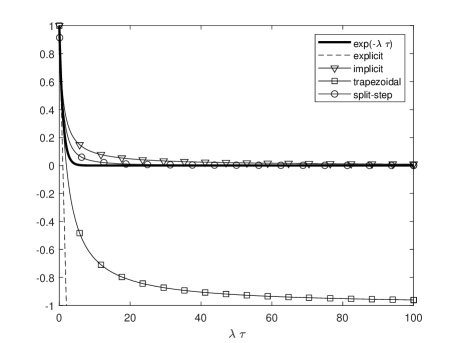
Table 1 shows the propagation coefficients and the stationary variance amplifiers of the theta scheme for different values of θ𝜃\displaystyle\theta. It is seen that the stationary mean of the true solution is recovered correctly for all values of θ𝜃\displaystyle\theta when condition (13) is satisfied. The stationary variance is resolved correctly only by the trapezoidal scheme with θ=12𝜃12\displaystyle\theta=\frac{1}{2}, other values of θ𝜃\displaystyle\theta result in either underdamped (θ<12𝜃12\displaystyle\theta<\frac{1}{2}) or overdamped (θ>12𝜃12\displaystyle\theta>\frac{1}{2}) variance. Additionally, one can see from Figure 1 that the propagation coefficient of the trapezoidal scheme is close to one for large values of λτ𝜆𝜏\displaystyle\lambda\tau indicating slow relaxation rate of the numerical solution to the stationary state. This limits the domain of application of the trapezoidal scheme to the systems with the time scale separation much larger than the relaxation time of the numerical solution.

θ𝜃\displaystyle\theta Propagation coefficients

1λ(1θ)τ1+λθτ1𝜆1𝜃𝜏1𝜆𝜃𝜏\displaystyle\frac{1-\lambda(1-\theta)\tau}{1+\lambda\theta\tau}
Variance amplifiers

22+λ(2θ1)τ22𝜆2𝜃1𝜏\displaystyle\frac{2}{2+\lambda(2\theta-1)\tau}
Stability condition
0 1λτ1𝜆𝜏\displaystyle 1-\lambda\tau 22λτ22𝜆𝜏\displaystyle\frac{2}{2-\lambda\tau} τ<2λ𝜏2𝜆\displaystyle\tau<\frac{{\color[rgb]{0,0,0}2}}{\lambda}
1212\displaystyle\frac{1}{2} 2λτ2+λτ2𝜆𝜏2𝜆𝜏\displaystyle\frac{2-\lambda\tau}{2+\lambda\tau} 1 unconditional
1 11+λτ11𝜆𝜏\displaystyle\frac{1}{1+\lambda\tau} 22+λτ22𝜆𝜏\displaystyle\frac{2}{2+\lambda\tau} unconditional
Table 1: Propagation coefficients and stationary variance amplifiers of the theta method (9). Parameter λ𝜆\displaystyle\lambda is set to λ=c1+c2𝜆subscript𝑐1subscript𝑐2\displaystyle\lambda=c_{1}+c_{2}.

Now consider the split-step method (3.2) applied to the system (12). Let θr=θsubscript𝜃𝑟𝜃\displaystyle\theta_{r}=\theta, η1r=η1subscript𝜂1𝑟subscript𝜂1\displaystyle\eta_{1r}=\eta_{1} and η2r=η2subscript𝜂2𝑟subscript𝜂2\displaystyle\eta_{2r}=\eta_{2}. The global stability condition reads as (see B)

|P(λτ)|=|(1(1η1)λ(1θ)τ1+η1λ(1θ)τ)(1(1η2)λθτ1+η2λθτ)|<1.𝑃𝜆𝜏11subscript𝜂1𝜆1𝜃𝜏1subscript𝜂1𝜆1𝜃𝜏11subscript𝜂2𝜆𝜃𝜏1subscript𝜂2𝜆𝜃𝜏1\displaystyle\displaystyle|P(\lambda\tau)|=\left|\left(\frac{1-(1-\eta_{1})\lambda(1-\theta)\tau}{1+\eta_{1}\lambda(1-\theta)\tau}\right)\left(\frac{1-(1-\eta_{2})\lambda\theta\tau}{1+\eta_{2}\lambda\theta\tau}\right)\right|<1.

Assuming this condition, the stationary moments of the numerical solution take the following values

𝔼[Y()]𝔼delimited-[]𝑌\displaystyle\displaystyle\mathbb{E}\left[{Y(\infty)}\right] =𝔼[X],absent𝔼delimited-[]superscript𝑋\displaystyle\displaystyle=\mathbb{E}\left[{X^{*}}\right],
𝕍ar[Y()]𝕍𝑎𝑟delimited-[]𝑌\displaystyle\displaystyle\mathbb{V}ar\left[{Y(\infty)}\right] =A(λτ)𝕍ar[X]absent𝐴𝜆𝜏𝕍𝑎𝑟delimited-[]superscript𝑋\displaystyle\displaystyle=A(\lambda\tau)\mathbb{V}ar\left[{X^{*}}\right]

with

A(λτ)=2λτ(1+η2λθτ1(1η2)λθτ)2(1(1η1)λ(1θ)τ1+η1λ(1θ)τ)2.𝐴𝜆𝜏2𝜆𝜏superscript1subscript𝜂2𝜆𝜃𝜏11subscript𝜂2𝜆𝜃𝜏2superscript11subscript𝜂1𝜆1𝜃𝜏1subscript𝜂1𝜆1𝜃𝜏2\displaystyle A(\lambda\tau)=\frac{2\lambda\tau}{\displaystyle{\left(\frac{1+\eta_{2}\lambda\theta\tau}{1-(1-\eta_{2})\lambda\theta\tau}\right)^{2}-\left(\frac{1-(1-\eta_{1})\lambda(1-\theta)\tau}{1+\eta_{1}\lambda(1-\theta)\tau}\right)^{2}}}.

One can see that the split-step method also preserves the stationary mean of the true solution while the stationary variance depends on the choice of the parameters θ𝜃\displaystyle\theta, η1subscript𝜂1\displaystyle\eta_{1}, η2subscript𝜂2\displaystyle\eta_{2}. Table 4.1 provides the propagation coefficients and the variance amplifiers of the scheme (3.2) for different values of these parameters. It is seen that the proposed scheme recovers the stability properties of the theta tau-leaping method when η1=0subscript𝜂10\displaystyle\eta_{1}=0, η2=1subscript𝜂21\displaystyle\eta_{2}=1 and of the standard split-step scheme (10) when θ=0𝜃0\displaystyle\theta=0, η1=1subscript𝜂11\displaystyle\eta_{1}=1. By rewriting the variance amplifier as a rational function in λτ𝜆𝜏\displaystyle\lambda\tau, it is also easy to check that the only choice of fixed parameters for which 𝕍ar[Y()]=𝕍ar[X]𝕍𝑎𝑟delimited-[]𝑌𝕍𝑎𝑟delimited-[]superscript𝑋\displaystyle\mathbb{V}ar\left[{Y(\infty)}\right]=\mathbb{V}ar\left[{X^{*}}\right] uniformly in λτ𝜆𝜏\displaystyle\lambda\tau is given by η1=0subscript𝜂10\displaystyle\eta_{1}=0, η2=1subscript𝜂21\displaystyle\eta_{2}=1, θ=12𝜃12\displaystyle\theta=\frac{1}{2} which corresponds to the trapezoidal theta scheme.

[θ,η1,η2]𝜃subscript𝜂1subscript𝜂2\displaystyle[\theta,\eta_{1},\eta_{2}] Propagation
coefficients Variance
amplifiers Stability
condition
[θ,1,1]𝜃11\displaystyle[\theta,1,1] 11+z+θ(1θ)z211𝑧𝜃1𝜃superscript𝑧2\displaystyle\frac{1}{1+z+\theta(1-\theta)z^{2}} 2z(1+θz)21(1+(1θ)z)22𝑧superscript1𝜃𝑧21superscript11𝜃𝑧2\displaystyle\frac{2z}{(1+\theta z)^{2}-\displaystyle{\frac{1}{(1+(1-\theta)z)^{2}}}} unconditional
[θ,0,1]𝜃01\displaystyle[\theta,0,1] 1(1θ)z1+θz11𝜃𝑧1𝜃𝑧\displaystyle\frac{1-(1-\theta)z}{1+\theta z} 22+(2θ1)z222𝜃1𝑧\displaystyle\frac{2}{2+(2\theta-1)z} (12θ)z<212𝜃𝑧2\displaystyle(1-2\theta)z<2
[0,η1,η2]0subscript𝜂1subscript𝜂2\displaystyle[0,\eta_{1},\eta_{2}] 1(1η1)z1+η1z11subscript𝜂1𝑧1subscript𝜂1𝑧\displaystyle\frac{1-(1-\eta_{1})z}{1+\eta_{1}z} 2(1+η1z)22+z(12η1+2η12)2superscript1subscript𝜂1𝑧22𝑧12subscript𝜂12superscriptsubscript𝜂12\displaystyle\frac{2(1+\eta_{1}z)^{2}}{2+z(1-2\eta_{1}+2\eta_{1}^{2})} (12η1)z<212subscript𝜂1𝑧2\displaystyle(1-2\eta_{1})z<2
Table 2: Propagation coefficients and stationary variance amplifiers of the split-step method (10) with z=λτ𝑧𝜆𝜏\displaystyle z=\lambda\tau and λ=c1+c2𝜆subscript𝑐1subscript𝑐2\displaystyle\lambda=c_{1}+c_{2}.

It is worth noting that with η1=η2=1subscript𝜂1subscript𝜂21\displaystyle\eta_{1}=\eta_{2}=1, the global stability condition for the split-step method is satisfied uniformly in θ𝜃\displaystyle\theta and the propagation coefficient tends to zero for large values of λτ𝜆𝜏\displaystyle\lambda\tau producing numerical solutions with small relaxation time. Figure 1 illustrates the propagation coefficients from Tables 1 and 4.1 for different numerical schemes along with the exponential decay eλtsuperscript𝑒𝜆𝑡\displaystyle e^{-\lambda t} of the exact mean 𝔼[X1(t)]𝔼delimited-[]subscript𝑋1𝑡\displaystyle\mathbb{E}\left[{X_{1}(t)}\right]. It is clear that the split-step method with η1=η2=1subscript𝜂1subscript𝜂21\displaystyle\eta_{1}=\eta_{2}=1 gives the best approximation of the true exponential decay when compared to other considered schemes. Moreover, by an appropriate choice of the parameter θ𝜃\displaystyle\theta, the scheme can reproduce the exact stationary variance of the true solution for each given λτ𝜆𝜏\displaystyle\lambda\tau. The following condition can ensure this

2λτ(1+θλτ)21(1+(1θ)λτ)2=1.2𝜆𝜏superscript1𝜃𝜆𝜏21superscript11𝜃𝜆𝜏21\displaystyle\displaystyle\frac{2\lambda\tau}{(1+\theta\lambda\tau)^{2}-\displaystyle{\frac{1}{(1+(1-\theta)\lambda\tau)^{2}}}}=1. (15)

The above equation does not have a closed form solution. However, for large values of λτ𝜆𝜏\displaystyle\lambda\tau, the fraction in the denominator can be neglected which gives the following approximation

θ= 2λτ-1λτ,   λ=c_1+c_2. For the small values of λτ𝜆𝜏\displaystyle\lambda\tau, one can search for the solution in the form of

θ𝜃\displaystyle\displaystyle\theta =θ+θ′′λτ+θ′′′(λτ)2+absentsuperscript𝜃superscript𝜃′′𝜆𝜏superscript𝜃′′′superscript𝜆𝜏2\displaystyle\displaystyle=\theta^{{}^{\prime}}+\theta^{{}^{\prime\prime}}\lambda\tau+\theta^{{}^{\prime\prime\prime}}(\lambda\tau)^{2}+...

Substituting this asymptotic expansion into the original equation and solving for the coefficients, we get

θsuperscript𝜃\displaystyle\displaystyle\theta^{{}^{\prime}} =332,θ′′=9+536,θ′′′=108187324,formulae-sequenceabsent332formulae-sequencesuperscript𝜃′′9536superscript𝜃′′′108187324\displaystyle\displaystyle=\frac{3-\sqrt{3}}{2},\quad\theta^{{}^{\prime\prime}}=\frac{-9+5\sqrt{3}}{6},\quad\theta^{{}^{\prime\prime\prime}}=\frac{108-187\sqrt{3}}{24},\quad...

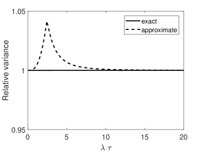
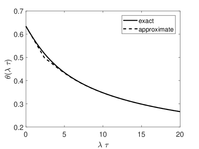
As can be seen from Figure 2, it is appropriate to choose the following representation for the parameter θ𝜃\displaystyle\theta

θ(λτ)={θ+θ′′λτ,if λτ2.45,2λτ1λτ,if λτ>2.45.𝜃𝜆𝜏casessuperscript𝜃superscript𝜃′′𝜆𝜏if 𝜆𝜏2.452𝜆𝜏1𝜆𝜏if 𝜆𝜏2.45\displaystyle\displaystyle\theta(\lambda\tau)=\begin{cases}\theta^{{}^{\prime}}+\theta^{{}^{\prime\prime}}\lambda\tau,&\text{if }\lambda\tau\leq 2.45,\\[10.00002pt] \sqrt{\frac{2}{\lambda\tau}}-\frac{1}{\lambda\tau},&\text{if }\lambda\tau>2.45.\end{cases} (16)

The value λτ=2.45𝜆𝜏2.45\displaystyle\lambda\tau=2.45 corresponds to the point where the two branches of θ(λτ)𝜃𝜆𝜏\displaystyle\theta(\lambda\tau) coincide.

Note that the above formula is obtained by fitting the asymptotical moments of the numerical solution to the exact stationary moments of the true solution. This approach is suitable only for simple systems with known analytical distributions. In the next section, we generalize this parameter estimation technique to arbitrary chemical networks.
Refer to caption
Figure 1: Propagation coefficient of numerical schemes.
Refer to caption
Refer to caption
Figure 2: Parameter θ𝜃\displaystyle\theta and the corresponding variance amplifier.

The parameter λ=c1+c2𝜆subscript𝑐1subscript𝑐2\displaystyle\lambda=c_{1}+c_{2} in the formula (16) is the measure of the relaxation rate of the reversible pair S1c1c2S2subscript𝑆1subscript𝑐2superscriptsubscript𝑐1subscript𝑆2\displaystyle S_{1}\underset{c_{2}}{\stackrel{{\scriptstyle c_{1}}}{{\rightleftharpoons}}}S_{2} to its stationary distribution. It can also be obtained through a deterministic analysis by studying the eigenvalues of the Jacobian matrix of the corresponding reaction rate equation. Indeed, the coefficient matrix of the linear differential system

ddt(z1z2)=(c1c2c1c2)(z1z2)𝑑𝑑𝑡matrixsubscript𝑧1subscript𝑧2matrixsubscript𝑐1subscript𝑐2subscript𝑐1subscript𝑐2matrixsubscript𝑧1subscript𝑧2\displaystyle\displaystyle\frac{d}{dt}\begin{pmatrix}z_{1}\\[5.0pt] z_{2}\end{pmatrix}=\begin{pmatrix}-c_{1}&c_{2}\\[5.0pt] c_{1}&-c_{2}\end{pmatrix}\begin{pmatrix}z_{1}\\[5.0pt] z_{2}\end{pmatrix}

has two eigenvalues: λ1=0subscript𝜆10\displaystyle\lambda_{1}=0 and λ2=c1c2subscript𝜆2subscript𝑐1subscript𝑐2\displaystyle\lambda_{2}=-c_{1}-c_{2}. In a general case, the system of RREs with an equilibrium point Xsuperscript𝑋\displaystyle X^{*} can be linearized around this point giving the system of ODEs

dedt=ν𝒟a(X)e,𝑑𝑒𝑑𝑡𝜈𝒟𝑎superscript𝑋𝑒\displaystyle\displaystyle\frac{de}{dt}=\nu\cdot\mathcal{D}a(X^{*})\cdot e,

where e=XX𝑒𝑋superscript𝑋\displaystyle e=X-X^{*} and 𝒟a(X)𝒟𝑎superscript𝑋\displaystyle\mathcal{D}a(X^{*}) is the Jacobian matrix of the vector with reaction propensities. For the reversible pairs of reactions, the rank of the stoichiometric matrix ν𝜈\displaystyle\nu is equal to one which, according to the rank-nullity theorem, implies that the coefficient matrix of the linearized system has exactly one non-zero eigenvalue. Since the trace of a matrix is the sum of its eigenvalues, the rate of decay of a reversible pair can be easily computed as

λ=Tr[ν𝒟a(X)],𝜆Tr𝜈𝒟𝑎superscript𝑋\displaystyle\displaystyle\lambda=-\operatorname{Tr}\big{[}\nu\cdot\mathcal{D}a(X^{*})\big{]}, (17)

where TrTr\displaystyle\operatorname{Tr} denotes the trace operator.

4.2 Parameter estimation for general systems

Recall that for the case of linear propensity functions in (4), the temporal evolution of the mean and covariance is described by the system of equations

t𝔼[X(t)]𝑡𝔼delimited-[]𝑋𝑡\displaystyle\displaystyle\frac{\partial}{\partial t}\mathbb{E}\left[{X(t)}\right] =νC𝔼[X(t)]+νd,absent𝜈𝐶𝔼delimited-[]𝑋𝑡𝜈𝑑\displaystyle\displaystyle=\nu C\cdot\mathbb{E}\left[{X(t)}\right]+\nu d, (5)
tov[X(t)]𝑡𝑜𝑣delimited-[]𝑋𝑡\displaystyle\displaystyle\frac{\partial}{\partial t}\mathbb{C}ov\left[{X(t)}\right] =νCov[X(t)]+ov[X(t)](νC)Tabsent𝜈𝐶𝑜𝑣delimited-[]𝑋𝑡𝑜𝑣delimited-[]𝑋𝑡superscript𝜈𝐶𝑇\displaystyle\displaystyle=\nu C\cdot\mathbb{C}ov\left[{X(t)}\right]+\mathbb{C}ov\left[{X(t)}\right]\cdot(\nu C)^{T} (6)
+νdiag(C𝔼[X(t)]+d)νT.𝜈𝑑𝑖𝑎𝑔𝐶𝔼delimited-[]𝑋𝑡𝑑superscript𝜈𝑇\displaystyle\displaystyle+\nu\cdot diag\left(C\cdot\mathbb{E}\left[{X(t)}\right]+d\right)\cdot\nu^{T}.

We use these equations to estimate the parameters of the split-step scheme by optimizing the error in the first two moments.

The key idea of the proposed approach can be broken down to three steps. Firstly, to find the reference values of the mean and covariance, we need to solve the system in (5)-(6) either analytically or numerically. When the analytical solution is not available, we find its numerical approximation by discretizing the above equations as follows

μn+1subscript𝜇𝑛1\displaystyle\displaystyle\mu_{n+1} =P1μn+τp2,absentsubscript𝑃1subscript𝜇𝑛𝜏subscript𝑝2\displaystyle\displaystyle=P_{1}\mu_{n}+\tau p_{2}, (18)
P3σn+1+σn+1P3Tsubscript𝑃3subscript𝜎𝑛1subscript𝜎𝑛1superscriptsubscript𝑃3𝑇\displaystyle\displaystyle P_{3}\sigma_{n+1}+\sigma_{n+1}P_{3}^{T} =P4σn+σnP4T+τνdiag(Cμn+1+d)νT,absentsubscript𝑃4subscript𝜎𝑛subscript𝜎𝑛superscriptsubscript𝑃4𝑇𝜏𝜈𝑑𝑖𝑎𝑔𝐶subscript𝜇𝑛1𝑑superscript𝜈𝑇\displaystyle\displaystyle=P_{4}\sigma_{n}+\sigma_{n}P_{4}^{T}+\tau\nu\cdot diag(C\mu_{n+1}+d)\cdot\nu^{T}, (19)

where μnsubscript𝜇𝑛\displaystyle\mu_{n} and σnsubscript𝜎𝑛\displaystyle\sigma_{n} are the numerical approximations of 𝔼[X(tn)]𝔼delimited-[]𝑋subscript𝑡𝑛\displaystyle\mathbb{E}\left[{X(t_{n})}\right] and ov[X(tn)]𝑜𝑣delimited-[]𝑋subscript𝑡𝑛\displaystyle\mathbb{C}ov\left[{X(t_{n})}\right] respectively. The coefficient matrices and vectors in the above formulas are given by

P1subscript𝑃1\displaystyle\displaystyle P_{1} =(Iθ~τνC)1(I+(1θ~)τνC),absentsuperscript𝐼~𝜃𝜏𝜈𝐶1𝐼1~𝜃𝜏𝜈𝐶\displaystyle\displaystyle=\Big{(}I-\tilde{\theta}\tau\nu C\Big{)}^{-1}\Big{(}I+(1-\tilde{\theta})\tau\nu C\Big{)},\qquad P3=12Iθ~τνC,subscript𝑃312𝐼~𝜃𝜏𝜈𝐶\displaystyle\displaystyle P_{3}=\frac{1}{2}I-\tilde{\theta}\tau\nu C,
p2subscript𝑝2\displaystyle\displaystyle p_{2} =(Iθ~τνC)1νd,absentsuperscript𝐼~𝜃𝜏𝜈𝐶1𝜈𝑑\displaystyle\displaystyle=\Big{(}I-\tilde{\theta}\tau\nu C\Big{)}^{-1}\nu d,\qquad P4=12I+(1θ~)τνC.subscript𝑃412𝐼1~𝜃𝜏𝜈𝐶\displaystyle\displaystyle P_{4}=\frac{1}{2}I+(1-\tilde{\theta})\tau\nu C.

Note that the parameter θ~~𝜃\displaystyle\tilde{\theta} above is in general not related to the parameter θ𝜃\displaystyle\theta in the considered split-step scheme (3.2). Any other approximation scheme for the solution of (5)-(6) can also be used instead of (18)-(19). Moreover, in all numerical simulations below, we used the fully implicit scheme with θ~=1~𝜃1\displaystyle\tilde{\theta}=1.

Secondly, we explicitly derive the equations for the mean and covariance of the solution generated with the split-step scheme (3.2). In the case of linear propensity functions, it reads as

Y^nsubscript^𝑌𝑛\displaystyle\displaystyle\hat{Y}_{n} =R1Yn+τr2,absentsubscript𝑅1subscript𝑌𝑛𝜏subscript𝑟2\displaystyle\displaystyle=R_{1}Y_{n}+\tau r_{2},
Y~nsubscript~𝑌𝑛\displaystyle\displaystyle\tilde{Y}_{n} =Y^n+ν𝒫((CY^n+d)τ)τ(νCY^n+νd),absentsubscript^𝑌𝑛𝜈𝒫𝐶subscript^𝑌𝑛𝑑𝜏𝜏𝜈𝐶subscript^𝑌𝑛𝜈𝑑\displaystyle\displaystyle=\hat{Y}_{n}+\nu\mathcal{P}\Big{(}\big{(}C\hat{Y}_{n}+d\big{)}\tau\Big{)}-\tau\Big{(}\nu C\hat{Y}_{n}+\nu d\Big{)}, (20)
Yn+1subscript𝑌𝑛1\displaystyle\displaystyle Y_{n+1} =R3Y~n+τr4,absentsubscript𝑅3subscript~𝑌𝑛𝜏subscript𝑟4\displaystyle\displaystyle=R_{3}\tilde{Y}_{n}+\tau r_{4},

where

R1subscript𝑅1\displaystyle\displaystyle R_{1} =(Iτνdiag(η1)diag(1θ)C)1(I+τνdiag(1η1)diag(1θ)C),absentsuperscript𝐼𝜏𝜈𝑑𝑖𝑎𝑔subscript𝜂1𝑑𝑖𝑎𝑔1𝜃𝐶1𝐼𝜏𝜈𝑑𝑖𝑎𝑔1subscript𝜂1𝑑𝑖𝑎𝑔1𝜃𝐶\displaystyle\displaystyle=\Big{(}I-\tau\nu\cdot diag(\eta_{1})\cdot diag(1-\theta)\cdot C\Big{)}^{-1}\Big{(}I+\tau\nu\cdot diag(1-\eta_{1})\cdot diag(1-\theta)\cdot C\Big{)},
r2subscript𝑟2\displaystyle\displaystyle r_{2} =(Iτνdiag(η1)diag(1θ)C)1νdiag(1θ)d,absentsuperscript𝐼𝜏𝜈𝑑𝑖𝑎𝑔subscript𝜂1𝑑𝑖𝑎𝑔1𝜃𝐶1𝜈𝑑𝑖𝑎𝑔1𝜃𝑑\displaystyle\displaystyle=\Big{(}I-\tau\nu\cdot diag(\eta_{1})\cdot diag(1-\theta)\cdot C\Big{)}^{-1}\nu\cdot diag(1-\theta)\cdot d,
R3subscript𝑅3\displaystyle\displaystyle R_{3} =(Iτνdiag(η2)diag(θ)C)1(I+τνdiag(1η2)diag(θ)C),absentsuperscript𝐼𝜏𝜈𝑑𝑖𝑎𝑔subscript𝜂2𝑑𝑖𝑎𝑔𝜃𝐶1𝐼𝜏𝜈𝑑𝑖𝑎𝑔1subscript𝜂2𝑑𝑖𝑎𝑔𝜃𝐶\displaystyle\displaystyle=\Big{(}I-\tau\nu\cdot diag(\eta_{2})\cdot diag(\theta)\cdot C\Big{)}^{-1}\Big{(}I+\tau\nu\cdot diag(1-\eta_{2})\cdot diag(\theta)\cdot C\Big{)},
r4subscript𝑟4\displaystyle\displaystyle r_{4} =(Iτνdiag(η2)diag(θ)C)1νdiag(θ)dabsentsuperscript𝐼𝜏𝜈𝑑𝑖𝑎𝑔subscript𝜂2𝑑𝑖𝑎𝑔𝜃𝐶1𝜈𝑑𝑖𝑎𝑔𝜃𝑑\displaystyle\displaystyle=\Big{(}I-\tau\nu\cdot diag(\eta_{2})\cdot diag(\theta)\cdot C\Big{)}^{-1}\nu\cdot diag(\theta)\cdot d

and θ=[θ1,,θR]T𝜃superscriptsubscript𝜃1subscript𝜃𝑅𝑇\displaystyle\theta=[\theta_{1},...,\theta_{R}]^{T}, η1=[η11,,η1R]Tsubscript𝜂1superscriptsubscript𝜂11subscript𝜂1𝑅𝑇\displaystyle\eta_{1}=[\eta_{11},...,\eta_{1R}]^{T}, η2=[η21,,η2R]Tsubscript𝜂2superscriptsubscript𝜂21subscript𝜂2𝑅𝑇\displaystyle\eta_{2}=[\eta_{21},...,\eta_{2R}]^{T}.

By applying Lemma 1, it is easy to show that the expectation of Yn+1subscript𝑌𝑛1\displaystyle Y_{n+1} is given by

𝔼[Y^n]𝔼delimited-[]subscript^𝑌𝑛\displaystyle\displaystyle\mathbb{E}\left[{\hat{Y}_{n}}\right] =R1𝔼[Yn]+τr2,absentsubscript𝑅1𝔼delimited-[]subscript𝑌𝑛𝜏subscript𝑟2\displaystyle\displaystyle=R_{1}\mathbb{E}\left[{Y_{n}}\right]+\tau r_{2},
𝔼[Yn+1]𝔼delimited-[]subscript𝑌𝑛1\displaystyle\displaystyle\mathbb{E}\left[{{Y}_{n+1}}\right] =R3𝔼[Y^n]+τr4.absentsubscript𝑅3𝔼delimited-[]subscript^𝑌𝑛𝜏subscript𝑟4\displaystyle\displaystyle=R_{3}\mathbb{E}\left[{\hat{Y}_{n}}\right]+\tau r_{4}. (21)

To find the covariance of Yn+1subscript𝑌𝑛1\displaystyle Y_{n+1}, recall that the components of the random vector 𝒫((CY^n+d)τ)𝒫𝐶subscript^𝑌𝑛𝑑𝜏\displaystyle\mathcal{P}\Big{(}\big{(}C\hat{Y}_{n}+d\big{)}\tau\Big{)} are independent Poisson variables conditioned on Ynsubscript𝑌𝑛\displaystyle Y_{n} and thus ov[𝒫((CY^n+d)τ)|Yn]𝑜𝑣delimited-[]conditional𝒫𝐶subscript^𝑌𝑛𝑑𝜏subscript𝑌𝑛\displaystyle\mathbb{C}ov\left[{\mathcal{P}\Big{(}\big{(}C\hat{Y}_{n}+d\big{)}\tau\Big{)}|Y_{n}}\right] is a diagonal matrix. This gives

ov[Y^n]𝑜𝑣delimited-[]subscript^𝑌𝑛\displaystyle\displaystyle\mathbb{C}ov\left[{\hat{Y}_{n}}\right] =R1ov[Yn]R1T,absentsubscript𝑅1𝑜𝑣delimited-[]subscript𝑌𝑛superscriptsubscript𝑅1𝑇\displaystyle\displaystyle=R_{1}\mathbb{C}ov\left[{Y_{n}}\right]R_{1}^{T},
ov[Y~n]𝑜𝑣delimited-[]subscript~𝑌𝑛\displaystyle\displaystyle\mathbb{C}ov\left[{\tilde{Y}_{n}}\right] =ov[Y^n]+τνdiag(C𝔼[Y^n]+d)νT,absent𝑜𝑣delimited-[]subscript^𝑌𝑛𝜏𝜈𝑑𝑖𝑎𝑔𝐶𝔼delimited-[]subscript^𝑌𝑛𝑑superscript𝜈𝑇\displaystyle\displaystyle=\mathbb{C}ov\left[{\hat{Y}_{n}}\right]+\tau\nu\cdot diag\left(C\mathbb{E}\left[{\hat{Y}_{n}}\right]+d\right)\cdot\nu^{T}, (22)
ov[Yn+1]𝑜𝑣delimited-[]subscript𝑌𝑛1\displaystyle\displaystyle\mathbb{C}ov\left[{Y_{n+1}}\right] =R3ov[Y~n]R3T.absentsubscript𝑅3𝑜𝑣delimited-[]subscript~𝑌𝑛superscriptsubscript𝑅3𝑇\displaystyle\displaystyle=R_{3}\mathbb{C}ov\left[{\tilde{Y}_{n}}\right]R_{3}^{T}.

Finally, by comparing the equations for the means in (5), (21) and covariances in (6), (22), we obtain the optimal parameter values θnsuperscript𝜃𝑛\displaystyle\theta^{n}, η1nsuperscriptsubscript𝜂1𝑛\displaystyle\eta_{1}^{n} and η2nsuperscriptsubscript𝜂2𝑛\displaystyle\eta_{2}^{n} at each time step as a solution to the following minimization problem

{θn,η1n,η2n}=argminθn,η1n,η2n[a,b](𝔼[Yn]μn2+ov[Yn]σnf2),superscript𝜃𝑛superscriptsubscript𝜂1𝑛superscriptsubscript𝜂2𝑛subscriptargminsuperscript𝜃𝑛superscriptsubscript𝜂1𝑛superscriptsubscript𝜂2𝑛𝑎𝑏superscriptnorm𝔼delimited-[]subscript𝑌𝑛subscript𝜇𝑛2superscriptsubscriptnorm𝑜𝑣delimited-[]subscript𝑌𝑛subscript𝜎𝑛𝑓2\displaystyle\displaystyle\{\theta^{n},\eta_{1}^{n},\eta_{2}^{n}\}=\operatorname*{arg\,min}_{\theta^{n},\eta_{1}^{n},\eta_{2}^{n}\in[a,b]}\Big{(}\left\|\mathbb{E}\left[{Y_{n}}\right]-\mu_{n}\right\|^{2}+\left\|\mathbb{C}ov\left[{Y_{n}}\right]-\sigma_{n}\right\|_{f}^{2}\Big{)}, (23)

where [a,b]𝑎𝑏\displaystyle[a,b] is a bounded interval, f\displaystyle\left\|\cdot\right\|_{f} is the Frobenius matrix norm and \displaystyle\left\|\cdot\right\| is the usual Euclidean vector norm. Algorithm 1 contains a detailed description of the proposed parameter estimation approach.

Algorithm 1 Parameter estimation for the split-step tau-leaping algorithm
0:  Initial condition X0subscript𝑋0\displaystyle X_{0}, time step τ𝜏\displaystyle\tau, final time T𝑇\displaystyle T, α1<1subscript𝛼11\displaystyle\alpha_{1}<1, α2<1subscript𝛼21\displaystyle\alpha_{2}<1
0:  Optimal parameter values
1:  for  each reversible reaction pair  do
2:     Estimate the relaxation rate λrsubscript𝜆𝑟\displaystyle\lambda_{r} using formula (17)
3:     Find θr0superscriptsubscript𝜃𝑟0\displaystyle\theta_{r}^{0} as a solution of the equation (15) or using formula (16)
4:     Set η1r0=η2r0=1superscriptsubscript𝜂1𝑟0superscriptsubscript𝜂2𝑟01\displaystyle\eta_{1r}^{0}=\eta_{2r}^{0}=1
5:  end for
6:  n1𝑛1\displaystyle n\leftarrow 1
7:  t1=t0+τsubscript𝑡1subscript𝑡0𝜏\displaystyle t_{1}=t_{0}+\tau
8:  while tnTsubscript𝑡𝑛𝑇\displaystyle t_{n}\leq T do
9:     Find μnsubscript𝜇𝑛\displaystyle\mu_{n} and σnsubscript𝜎𝑛\displaystyle\sigma_{n} from (18) and (19)
10:     Set C=𝒟a(μn)𝐶𝒟𝑎subscript𝜇𝑛\displaystyle C=\mathcal{D}a\big{(}\mu_{n}\big{)} and d=a(μn)Cμn𝑑𝑎subscript𝜇𝑛𝐶subscript𝜇𝑛\displaystyle d=a\big{(}\mu_{n}\big{)}-C\cdot\mu_{n}
11:     Set θn1,η1n1,η2n1superscript𝜃𝑛1superscriptsubscript𝜂1𝑛1superscriptsubscript𝜂2𝑛1\displaystyle\theta^{n-1},\eta_{1}^{n-1},\eta_{2}^{n-1} as initial guess for θn,η1n,η2nsuperscript𝜃𝑛superscriptsubscript𝜂1𝑛superscriptsubscript𝜂2𝑛\displaystyle\theta^{n},\eta_{1}^{n},\eta_{2}^{n}
12:     Find θn,η1n,η2nsuperscript𝜃𝑛superscriptsubscript𝜂1𝑛superscriptsubscript𝜂2𝑛\displaystyle\theta^{n},\eta_{1}^{n},\eta_{2}^{n} from
{θn,η1n,η2n}=argmin(𝔼[Yn]μn2+ov[Yn]σnf2)superscript𝜃𝑛superscriptsubscript𝜂1𝑛superscriptsubscript𝜂2𝑛argminsuperscriptnorm𝔼delimited-[]subscript𝑌𝑛subscript𝜇𝑛2superscriptsubscriptnorm𝑜𝑣delimited-[]subscript𝑌𝑛subscript𝜎𝑛𝑓2\displaystyle\displaystyle\{\theta^{n},\eta_{1}^{n},\eta_{2}^{n}\}=\operatorname*{arg\,min}\Big{(}\left\|\mathbb{E}\left[{Y_{n}}\right]-\mu_{n}\right\|^{2}+\left\|\mathbb{C}ov\left[{Y_{n}}\right]-\sigma_{n}\right\|_{f}^{2}\Big{)}
13:     with 𝔼[Yn]𝔼delimited-[]subscript𝑌𝑛\displaystyle\mathbb{E}\left[{Y_{n}}\right] and ov[Yn]𝑜𝑣delimited-[]subscript𝑌𝑛\displaystyle\mathbb{C}ov\left[{Y_{n}}\right] given by the formulas (21) and (22) respectively
14:     if  𝔼[Yn]μnμnα1norm𝔼delimited-[]subscript𝑌𝑛subscript𝜇𝑛normsubscript𝜇𝑛subscript𝛼1\displaystyle\frac{\left\|\mathbb{E}\left[{Y_{n}}\right]-\mu_{n}\right\|}{\left\|\mu_{n}\right\|}\geq\alpha_{1} or ov[Yn]σnfσnfα2subscriptnorm𝑜𝑣delimited-[]subscript𝑌𝑛subscript𝜎𝑛𝑓subscriptnormsubscript𝜎𝑛𝑓subscript𝛼2\displaystyle\frac{\left\|\mathbb{C}ov\left[{Y_{n}}\right]-\sigma_{n}\right\|_{f}}{\left\|\sigma_{n}\right\|_{f}}\geq\alpha_{2}  then
15:        Reduce τ𝜏\displaystyle\tau
16:     else
17:        nn+1𝑛𝑛1\displaystyle n\leftarrow n+1
18:     end if
19:     tn=tn1+τsubscript𝑡𝑛subscript𝑡𝑛1𝜏\displaystyle t_{n}=t_{n-1}+\tau
20:  end while

For nonlinear systems, one can use the following linearization

a(X)𝑎𝑋\displaystyle\displaystyle a(X) a(𝔼[X])+𝒟a(𝔼[X])(X𝔼[X]).absent𝑎𝔼delimited-[]𝑋𝒟𝑎𝔼delimited-[]𝑋𝑋𝔼delimited-[]𝑋\displaystyle\displaystyle\approx a\big{(}\mathbb{E}\left[{X}\right]\big{)}+\mathcal{D}a\big{(}\mathbb{E}\left[{X}\right]\big{)}\cdot\big{(}X-\mathbb{E}\left[{X}\right]\big{)}. (24)

By setting

C=D a(E_ [ X ] )   and   d=a( E_ [ X ] ) - C ⋅E_ [ X ] , this approximation allows applying Algorithm 1 to arbitrary chemical networks.

Remark. Special care must be taken when addressing the existence and uniqueness of the solution to the optimization problem in (23). The uniqueness part can be relaxed because any sufficiently small local minimum of the target functional can be taken as a solution. Also, the initial guess with η1=η2=1subscript𝜂1subscript𝜂21\displaystyle\eta_{1}=\eta_{2}=1 and θ𝜃\displaystyle\theta as in (16) (by considering reversible pairs individually in isolation from other reactions) often lies in the basin of attraction of the global minimum. The existence of the solution is also guaranteed because the problem is constrained to the bounded interval.

5 Numerical examples

In this section, we present numerical results for both linear and nonlinear problems. The provided examples aim to show that the proposed integration technique is capable to accurately recover stationary distributions of reaction networks without explicitly resolving their temporal scales. In all examples below, we estimated the parameters with the single run of the standard unconstrained gradient search with the initial conditions as in Algorithm 1. All simulations were performed using 106superscript106\displaystyle 10^{6} Monte Carlo samples.

5.1 Example 1. (Linear system)

Consider the monomolecular reaction network with three pairs of reversible reactions

S1c1c2S2c3c4S3c5c6S4.subscript𝑆1subscript𝑐2superscriptsubscript𝑐1subscript𝑆2subscript𝑐4superscriptsubscript𝑐3subscript𝑆3subscript𝑐6superscriptsubscript𝑐5subscript𝑆4\displaystyle\displaystyle S_{1}~{}\underset{c_{2}}{\stackrel{{\scriptstyle c_{1}}}{{\rightleftharpoons}}}~{}S_{2}~{}\underset{c_{4}}{\stackrel{{\scriptstyle c_{3}}}{{\rightleftharpoons}}}~{}S_{3}~{}\underset{c_{6}}{\stackrel{{\scriptstyle c_{5}}}{{\rightleftharpoons}}}~{}S_{4}. (25)

This network is described by the following stoichiometric matrix

ν=(110000111100001111000011)𝜈matrix110000111100001111000011\displaystyle\displaystyle\nu=\begin{pmatrix}-1&1&0&0&0&0\\[5.0pt] 1&-1&-1&1&0&0\\[5.0pt] 0&0&1&-1&-1&1\\[5.0pt] 0&0&0&0&1&-1\end{pmatrix}

and the corresponding propensity functions

α1(X(t))=c1X1(t),subscript𝛼1𝑋𝑡subscript𝑐1subscript𝑋1𝑡\displaystyle\displaystyle\alpha_{1}(X(t))=c_{1}X_{1}(t),\quad α2(X(t))=c2X2(t),subscript𝛼2𝑋𝑡subscript𝑐2subscript𝑋2𝑡\displaystyle\displaystyle\alpha_{2}(X(t))=c_{2}X_{2}(t),
α3(X(t))=c3X2(t),subscript𝛼3𝑋𝑡subscript𝑐3subscript𝑋2𝑡\displaystyle\displaystyle\alpha_{3}(X(t))=c_{3}X_{2}(t),\quad α4(X(t))=c4X3(t),subscript𝛼4𝑋𝑡subscript𝑐4subscript𝑋3𝑡\displaystyle\displaystyle\alpha_{4}(X(t))=c_{4}X_{3}(t),
α5(X(t))=c5X3(t),subscript𝛼5𝑋𝑡subscript𝑐5subscript𝑋3𝑡\displaystyle\displaystyle\alpha_{5}(X(t))=c_{5}X_{3}(t),\quad α6(X(t))=c6X4(t).subscript𝛼6𝑋𝑡subscript𝑐6subscript𝑋4𝑡\displaystyle\displaystyle\alpha_{6}(X(t))=c_{6}X_{4}(t).

Monomolecular reactions provide an example of chemical systems with known analytical solutions [8]. For the initial condition X(0)=[xT,0,,0]T𝑋0superscriptsubscript𝑥𝑇00𝑇\displaystyle X(0)=[x_{T},0,...,0]^{T}, the exact distribution of X(t)𝑋𝑡\displaystyle X(t) is multinomial and has the particularly simple form

t,xsubscript𝑡𝑥\displaystyle\displaystyle\mathbb{P}_{t,x} =(x,xT,p(t)),p(t)=exp(tνC)[1,0,,0]T.formulae-sequenceabsent𝑥subscript𝑥𝑇𝑝𝑡𝑝𝑡𝑡𝜈𝐶superscript100𝑇\displaystyle\displaystyle=\mathcal{M}\big{(}x,x_{T},p(t)\big{)},\qquad p(t)=\exp(t\nu C)\cdot[1,0,...,0]^{T}.

The exact mean and covariance are thus given by
𝔼[X(t)]𝔼delimited-[]𝑋𝑡\displaystyle\displaystyle\mathbb{E}\left[{X(t)}\right] =xTp(t),absentsubscript𝑥𝑇𝑝𝑡\displaystyle\displaystyle=x_{T}\cdot p(t),
ov[Xi(t),Xj(t)]𝑜𝑣subscript𝑋𝑖𝑡subscript𝑋𝑗𝑡\displaystyle\displaystyle\mathbb{C}ov\left[{X_{i}(t),X_{j}(t)}\right] ={xTpi(t)(1pi(t))if i=j,xTpi(t)pj(t)if ij.absentcasessubscript𝑥𝑇subscript𝑝𝑖𝑡1subscript𝑝𝑖𝑡if 𝑖𝑗subscript𝑥𝑇subscript𝑝𝑖𝑡subscript𝑝𝑗𝑡if 𝑖𝑗\displaystyle\displaystyle=\begin{cases}x_{T}\cdot p_{i}(t)(1-p_{i}(t))&\text{if }i=j,\\ x_{T}\cdot p_{i}(t)p_{j}(t)&\text{if }i\neq j.\end{cases}
Refer to caption
Refer to caption
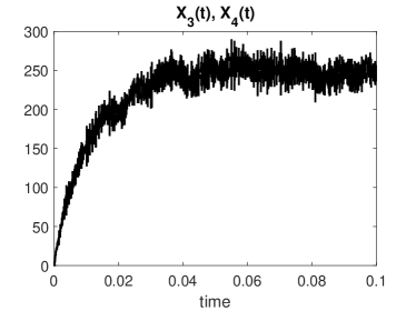
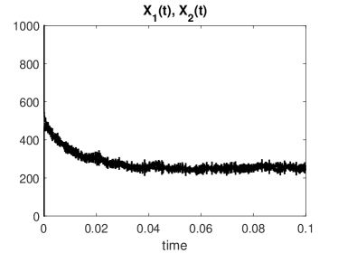
Figure 3: A realization of the state paths of the system in (25) with the initial condition X(0)=[1000,0,0,0]T𝑋0superscript1000000𝑇\displaystyle X(0)=[1000,0,0,0]^{T} and reaction rates c=[104,104,102,102,105,105]𝑐superscript104superscript104superscript102superscript102superscript105superscript105\displaystyle c~{}=~{}[10^{4},10^{4},10^{2},10^{2},10^{5},10^{5}].
[Uncaptioned image]
[Uncaptioned image]
[Uncaptioned image]
[Uncaptioned image]
Figure 4: Evolution of the mean and covariance of the system in (25) with the initial condition X(0)=[1000,0,0,0]T𝑋0superscript1000000𝑇\displaystyle X(0)=[1000,0,0,0]^{T} and reaction rates c=[104,104,102,102,105,105]𝑐superscript104superscript104superscript102superscript102superscript105superscript105\displaystyle c~{}=~{}[10^{4},10^{4},10^{2},10^{2},10^{5},10^{5}].

Figure 3 shows a single realization of the state paths for the stiff system in (25). The temporal evolution of some of the moments is depicted in Figure 4.1. It also shows the approximate moments calculated from the systems in (18)-(19) and (21)-(22). It is seen that the parameter estimation approach in (23) works well and both approximate solutions tend to the stationary state of the true analytical solution as desired.

To test the accuracy of the integrators, we fix the time step τ=1𝜏1\displaystyle\tau=1 and the final time T=100𝑇100\displaystyle T=100 and consider the reaction rates of the form

c=α[1,1,1,1,1,1]T.𝑐𝛼superscript111111𝑇\displaystyle\displaystyle c=\alpha\cdot[1,1,1,1,1,1]^{T}.

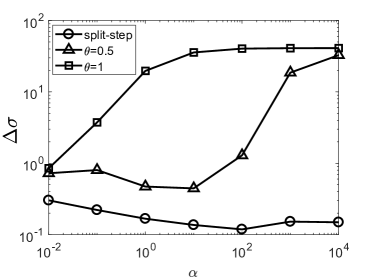
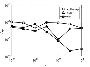
Different values of α𝛼\displaystyle\alpha allow to compare the performance of the proposed and classical methods at different temporal scales. Figure 5 illustrates the results of this comparison for the split-step algorithm in (10) and the theta scheme in (9). It is clear that both methods give accurate results for the stationary mean. However, the ability of the theta scheme to preserve the stationary variance is deteriorating at faster scales while the split-step method demonstrates the same level of accuracy uniformly in α𝛼\displaystyle\alpha. Also, note that the proposed algorithm has two implicit steps and is more expensive than the theta scheme using the same temporal discretization. However, the results in Figure 5 indicate that the split-step method is much more accurate and is more appropriate for simulating fast reactions.

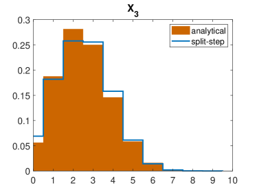
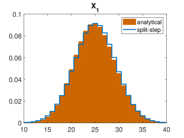
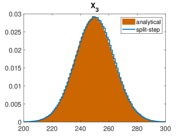
Finally, Figure 4.1 shows the exact and simulated marginal distributions of X1(T)subscript𝑋1𝑇\displaystyle X_{1}(T) and X3(T)subscript𝑋3𝑇\displaystyle X_{3}(T) for different numbers of molecules xTsubscript𝑥𝑇\displaystyle x_{T}. One can see that the split-step method (10) is able to accurately recover the stationary distributions for both small and large numbers of molecular species. The better accuracy for larger values of xTsubscript𝑥𝑇\displaystyle x_{T} can be explained as an artifact of the integrality preserving procedure.
Refer to caption
Refer to caption
Figure 5: Errors of the mean (left) and the covariance (right) of the simulated approximate solutions at T=100𝑇100\displaystyle T=100 for the reaction rates c=α[1,1,1,1,1,1]𝑐𝛼111111\displaystyle c~{}=\alpha\cdot[1,1,1,1,1,1].
Refer to caption
Refer to caption
(a) xT=10subscript𝑥𝑇10\displaystyle x_{T}=10
Refer to caption
Refer to caption
(b) xT=100subscript𝑥𝑇100\displaystyle x_{T}=100
Refer to caption
Refer to caption
(c) xT=1000subscript𝑥𝑇1000\displaystyle x_{T}=1000
Figure 6: Marginal distributions of X1(T)subscript𝑋1𝑇\displaystyle X_{1}(T) and X3(T)subscript𝑋3𝑇\displaystyle X_{3}(T) at T=10𝑇10\displaystyle T=10 for the system in (25) with the reaction rates c=[104,104,102,102,105,105].𝑐superscript104superscript104superscript102superscript102superscript105superscript105\displaystyle c~{}=~{}[10^{4},10^{4},10^{2},10^{2},10^{5},10^{5}].

5.2 Example 2. (Nonlinear system)

Consider the following stiff 3-species 6-reaction system [52]

S1+S2c1c2S3,subscript𝑆1subscript𝑆2subscript𝑐2superscriptsubscript𝑐1subscript𝑆3\displaystyle\displaystyle S_{1}+S_{2}\underset{c_{2}}{\stackrel{{\scriptstyle c_{1}}}{{\rightleftharpoons}}}S_{3},
S1+S3c3c4S2,subscript𝑆1subscript𝑆3subscript𝑐4superscriptsubscript𝑐3subscript𝑆2\displaystyle\displaystyle S_{1}+S_{3}\underset{c_{4}}{\stackrel{{\scriptstyle c_{3}}}{{\rightleftharpoons}}}S_{2}, (26)
S2+S3c5c6S1subscript𝑆2subscript𝑆3subscript𝑐6superscriptsubscript𝑐5subscript𝑆1\displaystyle\displaystyle S_{2}+S_{3}\underset{c_{6}}{\stackrel{{\scriptstyle c_{5}}}{{\rightleftharpoons}}}S_{1}

with the rate constants c1=c2=103subscript𝑐1subscript𝑐2superscript103\displaystyle c_{1}=c_{2}=10^{3}, c3=105subscript𝑐3superscript105\displaystyle c_{3}=10^{-5}, c4=10subscript𝑐410\displaystyle c_{4}=10, c5=1subscript𝑐51\displaystyle c_{5}=1 and c6=106subscript𝑐6superscript106\displaystyle c_{6}=10^{6}. The stoichiometric matrix of this reaction network is given by

ν=(111111111111111111)𝜈matrix111111111111111111\displaystyle\displaystyle\nu=\begin{pmatrix}-1&1&-1&1&1&-1\\[5.0pt] -1&1&1&-1&-1&1\\[5.0pt] 1&-1&-1&1&-1&1\\ \end{pmatrix}

and the propensities of the reaction channels are, respectively,

α1(X(t))=c1X1(t)X2(t),subscript𝛼1𝑋𝑡subscript𝑐1subscript𝑋1𝑡subscript𝑋2𝑡\displaystyle\displaystyle\alpha_{1}(X(t))=c_{1}X_{1}(t)X_{2}(t),\quad α2(X(t))=c2X3(t),subscript𝛼2𝑋𝑡subscript𝑐2subscript𝑋3𝑡\displaystyle\displaystyle\alpha_{2}(X(t))=c_{2}X_{3}(t),
α3(X(t))=c3X1(t)X3(t),subscript𝛼3𝑋𝑡subscript𝑐3subscript𝑋1𝑡subscript𝑋3𝑡\displaystyle\displaystyle\alpha_{3}(X(t))=c_{3}X_{1}(t)X_{3}(t),\quad α4(X(t))=c4X2(t),subscript𝛼4𝑋𝑡subscript𝑐4subscript𝑋2𝑡\displaystyle\displaystyle\alpha_{4}(X(t))=c_{4}X_{2}(t),
α5(X(t))=c5X2(t)X3(t),subscript𝛼5𝑋𝑡subscript𝑐5subscript𝑋2𝑡subscript𝑋3𝑡\displaystyle\displaystyle\alpha_{5}(X(t))=c_{5}X_{2}(t)X_{3}(t),\quad α6(X(t))=c6X1(t).subscript𝛼6𝑋𝑡subscript𝑐6subscript𝑋1𝑡\displaystyle\displaystyle\alpha_{6}(X(t))=c_{6}X_{1}(t).

The system in (5.2) does not have known analytical solutions. Instead, the reference solution was obtained using the stochastic simulation algorithm with 104superscript104\displaystyle 10^{4} samples. We used the initial condition X(0)=[103,103,106]T𝑋0superscriptsuperscript103superscript103superscript106𝑇\displaystyle X(0)=[10^{3},10^{3},10^{6}]^{T} which corresponds to the true stationary mean of this particular system and performed all simulations over the time interval [0,0.01]00.01\displaystyle[0,0.01] with the time step τ=103𝜏superscript103\displaystyle\tau=10^{-3}.

Figure 4.1 depicts the evolution in time of the selected elements of the mean vector and the covariance matrix. The approximate mean and covariance were evaluated using the linearization in (24). It is seen that both the linearization (24) and the corresponding fitted approximation (21)-(22) produce an adequate description of the true stationary nonlinear dynamics.

Additionally, Figure 4.1 provides the comparison of the marginal distributions obtained with the split-step and theta schemes. It is evident that both implicit and trapezoidal methods produce severely overdamped solutions resulting in very atomic distributions. At the same time, the proposed split-step integrator generates results which compare well to the reference solution as desired.

[Uncaptioned image]
[Uncaptioned image]
[Uncaptioned image]
[Uncaptioned image]
Figure 7: Evolution in time of the mean and covariance of the system in (5.2).
[Uncaptioned image]
[Uncaptioned image]
[Uncaptioned image]
[Uncaptioned image]
Figure 8: Marginal distributions of X1(T)subscript𝑋1𝑇\displaystyle X_{1}(T) and X3(T)subscript𝑋3𝑇\displaystyle X_{3}(T) at T=0.01𝑇0.01\displaystyle T=0.01 for the system in (5.2).

6 Conclusion

In this paper, we considered the problem of accurate integration of the fast and stable reactions using time discretizations much exceeding their scale. For this purpose, we proposed the new splitting heuristic for the tau-leaping method and devised the algorithm for the estimation of its parameters. We showed that the proposed integrator is stable and is capable to accurately sample from the stationary distributions of the fast molecular species at least in the linear case. Classical tau-leaping approximations do not possess this property and behave poorly as stiff integrators.

Appendix A Stability of the theta method

Let Ynsubscript𝑌𝑛\displaystyle Y_{n} denote the numerical approximation of X1(tn)subscript𝑋1subscript𝑡𝑛\displaystyle X_{1}(t_{n}) and consider the theta method (9) applied to the test system (12)

Yn+1subscript𝑌𝑛1\displaystyle\displaystyle Y_{n+1} =Yn+(c2(xTYn+1)c1Yn+1c2(xTYn)+c1Yn)θτabsentsubscript𝑌𝑛subscript𝑐2subscript𝑥𝑇subscript𝑌𝑛1subscript𝑐1subscript𝑌𝑛1subscript𝑐2subscript𝑥𝑇subscript𝑌𝑛subscript𝑐1subscript𝑌𝑛𝜃𝜏\displaystyle\displaystyle=Y_{n}+\Big{(}c_{2}(x_{T}-Y_{n+1})-c_{1}Y_{n+1}-c_{2}(x_{T}-Y_{n})+c_{1}Y_{n}\Big{)}\theta\tau
+𝒫(c2(xTYn)τ)𝒫(c1Ynτ)𝒫subscript𝑐2subscript𝑥𝑇subscript𝑌𝑛𝜏𝒫subscript𝑐1subscript𝑌𝑛𝜏\displaystyle\displaystyle+\mathcal{P}\Big{(}c_{2}(x_{T}-Y_{n})\tau\Big{)}-\mathcal{P}\Big{(}c_{1}Y_{n}\tau\Big{)}
=Yn+11+(c1+c2)θτ[𝒫(c2(xTYn)τ)𝒫(c1Ynτ)].absentsubscript𝑌𝑛11subscript𝑐1subscript𝑐2𝜃𝜏delimited-[]𝒫subscript𝑐2subscript𝑥𝑇subscript𝑌𝑛𝜏𝒫subscript𝑐1subscript𝑌𝑛𝜏\displaystyle\displaystyle=Y_{n}+\frac{1}{1+(c_{1}+c_{2})\theta\tau}\left[\mathcal{P}\Big{(}c_{2}(x_{T}-Y_{n})\tau\Big{)}-\mathcal{P}\Big{(}c_{1}Y_{n}\tau\Big{)}\right].

The mean and the variance of the solution obtained with the theta method can be easily calculated as

𝔼[Yn+1]𝔼delimited-[]subscript𝑌𝑛1\displaystyle\displaystyle\mathbb{E}\left[{Y_{n+1}}\right] =𝔼[𝔼[Yn+1|Yn]]absent𝔼delimited-[]𝔼delimited-[]conditionalsubscript𝑌𝑛1subscript𝑌𝑛\displaystyle\displaystyle=\mathbb{E}\left[{\mathbb{E}\left[{Y_{n+1}|Y_{n}}\right]}\right]
=𝔼[Yn+c2(xTYn)τc1Ynτ1+(c1+c2)θτ]=1(c1+c2)(1θ)τ1+(c1+c2)θτ𝔼[Yn]+c2xTτ1+(c1+c2)θτabsent𝔼delimited-[]subscript𝑌𝑛subscript𝑐2subscript𝑥𝑇subscript𝑌𝑛𝜏subscript𝑐1subscript𝑌𝑛𝜏1subscript𝑐1subscript𝑐2𝜃𝜏1subscript𝑐1subscript𝑐21𝜃𝜏1subscript𝑐1subscript𝑐2𝜃𝜏𝔼delimited-[]subscript𝑌𝑛subscript𝑐2subscript𝑥𝑇𝜏1subscript𝑐1subscript𝑐2𝜃𝜏\displaystyle\displaystyle=\mathbb{E}\left[{Y_{n}+\frac{c_{2}(x_{T}-Y_{n})\tau-c_{1}Y_{n}\tau}{1+(c_{1}+c_{2})\theta\tau}}\right]=\frac{1-(c_{1}+c_{2})(1-\theta)\tau}{1+(c_{1}+c_{2})\theta\tau}\mathbb{E}\left[{Y_{n}}\right]+\frac{c_{2}x_{T}\tau}{1+(c_{1}+c_{2})\theta\tau}

and

𝕍ar[Yn+1]𝕍𝑎𝑟delimited-[]subscript𝑌𝑛1\displaystyle\displaystyle\mathbb{V}ar\left[{Y_{n+1}}\right] =𝕍ar[𝔼[Yn+1|Yn]]+𝔼[𝕍ar[Yn+1|Yn]]absent𝕍𝑎𝑟delimited-[]𝔼delimited-[]conditionalsubscript𝑌𝑛1subscript𝑌𝑛𝔼delimited-[]𝕍𝑎𝑟delimited-[]conditionalsubscript𝑌𝑛1subscript𝑌𝑛\displaystyle\displaystyle=\mathbb{V}ar\left[{\mathbb{E}\left[{Y_{n+1}|Y_{n}}\right]}\right]+\mathbb{E}\left[{\mathbb{V}ar\left[{Y_{n+1}|Y_{n}}\right]}\right]
=𝕍ar[Yn+c2(xTYn)τc1Ynτ1+(c1+c2)θτ]+𝔼[c1Ynτ+c2(xTYn)τ(1+(c1+c2)θτ)2]absent𝕍𝑎𝑟delimited-[]subscript𝑌𝑛subscript𝑐2subscript𝑥𝑇subscript𝑌𝑛𝜏subscript𝑐1subscript𝑌𝑛𝜏1subscript𝑐1subscript𝑐2𝜃𝜏𝔼delimited-[]subscript𝑐1subscript𝑌𝑛𝜏subscript𝑐2subscript𝑥𝑇subscript𝑌𝑛𝜏superscript1subscript𝑐1subscript𝑐2𝜃𝜏2\displaystyle\displaystyle=\mathbb{V}ar\left[{Y_{n}+\frac{c_{2}(x_{T}-Y_{n})\tau-c_{1}Y_{n}\tau}{1+(c_{1}+c_{2})\theta\tau}}\right]+\mathbb{E}\left[{\frac{c_{1}Y_{n}\tau+c_{2}(x_{T}-Y_{n})\tau}{(1+(c_{1}+c_{2})\theta\tau)^{2}}}\right]
=(1(c1+c2)(1θ)τ1+(c1+c2)θτ)2𝕍ar[Yn]+(c1c2)τ(1+(c1+c2)θτ)2𝔼[Yn]+c2xTτ(1+(c1+c2)θτ)2.absentsuperscript1subscript𝑐1subscript𝑐21𝜃𝜏1subscript𝑐1subscript𝑐2𝜃𝜏2𝕍𝑎𝑟delimited-[]subscript𝑌𝑛subscript𝑐1subscript𝑐2𝜏superscript1subscript𝑐1subscript𝑐2𝜃𝜏2𝔼delimited-[]subscript𝑌𝑛subscript𝑐2subscript𝑥𝑇𝜏superscript1subscript𝑐1subscript𝑐2𝜃𝜏2\displaystyle\displaystyle=\left(\frac{1-(c_{1}+c_{2})(1-\theta)\tau}{1+(c_{1}+c_{2})\theta\tau}\right)^{2}\mathbb{V}ar\left[{Y_{n}}\right]+\frac{(c_{1}-c_{2})\tau}{(1+(c_{1}+c_{2})\theta\tau)^{2}}\mathbb{E}\left[{Y_{n}}\right]+\frac{c_{2}x_{T}\tau}{(1+(c_{1}+c_{2})\theta\tau)^{2}}.

These recurrences have the solutions

𝔼[Yn]𝔼delimited-[]subscript𝑌𝑛\displaystyle\displaystyle\mathbb{E}\left[{Y_{n}}\right] =An𝔼[Y0]+1An1AB,absentsuperscript𝐴𝑛𝔼delimited-[]subscript𝑌01superscript𝐴𝑛1𝐴𝐵\displaystyle\displaystyle=A^{n}\mathbb{E}\left[{Y_{0}}\right]+\frac{1-A^{n}}{1-A}B,
𝕍ar[Yn]𝕍𝑎𝑟delimited-[]subscript𝑌𝑛\displaystyle\displaystyle\mathbb{V}ar\left[{Y_{n}}\right] =A2n𝕍ar[Y0]+CA1An1A(𝔼[Yn]B1A)+1A2n1A2(BC1A+D),absentsuperscript𝐴2𝑛𝕍𝑎𝑟delimited-[]subscript𝑌0𝐶𝐴1superscript𝐴𝑛1𝐴𝔼delimited-[]subscript𝑌𝑛𝐵1𝐴1superscript𝐴2𝑛1superscript𝐴2𝐵𝐶1𝐴𝐷\displaystyle\displaystyle=A^{2n}\mathbb{V}ar\left[{Y_{0}}\right]+\frac{C}{A}\frac{1-A^{n}}{1-A}\left(\mathbb{E}\left[{Y_{n}}\right]-\frac{B}{1-A}\right)+\frac{1-A^{2n}}{1-A^{2}}\left(\frac{BC}{1-A}+D\right),

where the coefficients A𝐴\displaystyle A, B𝐵\displaystyle B, C𝐶\displaystyle C and D𝐷\displaystyle D are given by

A=1(c1+c2)(1θ)τ1+(c1+c2)θτ,𝐴1subscript𝑐1subscript𝑐21𝜃𝜏1subscript𝑐1subscript𝑐2𝜃𝜏\displaystyle\displaystyle A=\frac{1-(c_{1}+c_{2})(1-\theta)\tau}{1+(c_{1}+c_{2})\theta\tau},\qquad B=c2xTτ1+(c1+c2)θτ,𝐵subscript𝑐2subscript𝑥𝑇𝜏1subscript𝑐1subscript𝑐2𝜃𝜏\displaystyle\displaystyle B=\frac{c_{2}x_{T}\tau}{1+(c_{1}+c_{2})\theta\tau},
C=(c1c2)τ(1+(c1+c2)θτ)2,𝐶subscript𝑐1subscript𝑐2𝜏superscript1subscript𝑐1subscript𝑐2𝜃𝜏2\displaystyle\displaystyle C=\frac{(c_{1}-c_{2})\tau}{(1+(c_{1}+c_{2})\theta\tau)^{2}},\qquad D=c2xTτ(1+(c1+c2)θτ)2.𝐷subscript𝑐2subscript𝑥𝑇𝜏superscript1subscript𝑐1subscript𝑐2𝜃𝜏2\displaystyle\displaystyle D=\frac{c_{2}x_{T}\tau}{(1+(c_{1}+c_{2})\theta\tau)^{2}}.

The following condition ensures the global stability of the mean and the variance of the numerical solution obtained with the theta method (9)

|A|=|1(c1+c2)(1θ)τ1+(c1+c2)θτ|<1.𝐴1subscript𝑐1subscript𝑐21𝜃𝜏1subscript𝑐1subscript𝑐2𝜃𝜏1\displaystyle\displaystyle|A|=\left|\frac{1-(c_{1}+c_{2})(1-\theta)\tau}{1+(c_{1}+c_{2})\theta\tau}\right|<1.

Appendix B Stability of the split-step method

Let Ynsubscript𝑌𝑛\displaystyle Y_{n} denote the numerical approximation of X1(tn)subscript𝑋1subscript𝑡𝑛\displaystyle X_{1}(t_{n}) and consider the split-step method (3.2) applied to the test system (12)

Y^nsubscript^𝑌𝑛\displaystyle\displaystyle\hat{Y}_{n} =1(1η1)(c1+c2)(1θ)τ1+η1(c1+c2)(1θ)τYn+c2xT(1θ)τ1+η1(c1+c2)(1θ)τ,absent11subscript𝜂1subscript𝑐1subscript𝑐21𝜃𝜏1subscript𝜂1subscript𝑐1subscript𝑐21𝜃𝜏subscript𝑌𝑛subscript𝑐2subscript𝑥𝑇1𝜃𝜏1subscript𝜂1subscript𝑐1subscript𝑐21𝜃𝜏\displaystyle\displaystyle=\frac{1-(1-\eta_{1})(c_{1}+c_{2})(1-\theta)\tau}{1+\eta_{1}(c_{1}+c_{2})(1-\theta)\tau}Y_{n}+\frac{c_{2}x_{T}(1-\theta)\tau}{1+\eta_{1}(c_{1}+c_{2})(1-\theta)\tau},
Y~nsubscript~𝑌𝑛\displaystyle\displaystyle\tilde{Y}_{n} =(1+τ(c1+c2))Y^n+𝒫(c2(xTY^n)τ)𝒫(c1Y^nτ)c2τxT,absent1𝜏subscript𝑐1subscript𝑐2subscript^𝑌𝑛𝒫subscript𝑐2subscript𝑥𝑇subscript^𝑌𝑛𝜏𝒫subscript𝑐1subscript^𝑌𝑛𝜏subscript𝑐2𝜏subscript𝑥𝑇\displaystyle\displaystyle=(1+\tau(c_{1}+c_{2}))\hat{Y}_{n}+\mathcal{P}\left(c_{2}(x_{T}-\hat{Y}_{n})\tau\right)-\mathcal{P}\left(c_{1}\hat{Y}_{n}\tau\right)-c_{2}\tau x_{T},
Yn+1subscript𝑌𝑛1\displaystyle\displaystyle Y_{n+1} =1(1η2)(c1+c2)θτ1+η2(c1+c2)θτY~n+c2xTθτ1+η2(c1+c2)θτ.absent11subscript𝜂2subscript𝑐1subscript𝑐2𝜃𝜏1subscript𝜂2subscript𝑐1subscript𝑐2𝜃𝜏subscript~𝑌𝑛subscript𝑐2subscript𝑥𝑇𝜃𝜏1subscript𝜂2subscript𝑐1subscript𝑐2𝜃𝜏\displaystyle\displaystyle=\frac{1-(1-\eta_{2})(c_{1}+c_{2})\theta\tau}{1+\eta_{2}(c_{1}+c_{2})\theta\tau}\tilde{Y}_{n}+\frac{c_{2}x_{T}\theta\tau}{1+\eta_{2}(c_{1}+c_{2})\theta\tau}.

Equations for the mean and the variance take the form

𝔼[Yn+1]𝔼delimited-[]subscript𝑌𝑛1\displaystyle\displaystyle\mathbb{E}\left[{Y_{n+1}}\right] =(1(1η1)(c1+c2)(1θ)τ1+η1(c1+c2)(1θ)τ)(1(1η2)(c1+c2)θτ1+η2(c1+c2)θτ)𝔼[Yn]absent11subscript𝜂1subscript𝑐1subscript𝑐21𝜃𝜏1subscript𝜂1subscript𝑐1subscript𝑐21𝜃𝜏11subscript𝜂2subscript𝑐1subscript𝑐2𝜃𝜏1subscript𝜂2subscript𝑐1subscript𝑐2𝜃𝜏𝔼delimited-[]subscript𝑌𝑛\displaystyle\displaystyle=\left(\frac{1-(1-\eta_{1})(c_{1}+c_{2})(1-\theta)\tau}{1+\eta_{1}(c_{1}+c_{2})(1-\theta)\tau}\right)\left(\frac{1-(1-\eta_{2})(c_{1}+c_{2})\theta\tau}{1+\eta_{2}(c_{1}+c_{2})\theta\tau}\right)\mathbb{E}\left[{Y_{n}}\right]
+1(1η1η2)(c1+c2)θ(1θ)τ(1+η1(c1+c2)(1θ)τ)(1+η2(c1+c2)θτ)c2xTτ,11subscript𝜂1subscript𝜂2subscript𝑐1subscript𝑐2𝜃1𝜃𝜏1subscript𝜂1subscript𝑐1subscript𝑐21𝜃𝜏1subscript𝜂2subscript𝑐1subscript𝑐2𝜃𝜏subscript𝑐2subscript𝑥𝑇𝜏\displaystyle\displaystyle+\frac{1-(1-\eta_{1}-\eta_{2})(c_{1}+c_{2})\theta(1-\theta)\tau}{\Big{(}1+\eta_{1}(c_{1}+c_{2})(1-\theta)\tau\Big{)}\Big{(}1+\eta_{2}(c_{1}+c_{2})\theta\tau\Big{)}}c_{2}x_{T}\tau,
𝕍ar[Yn+1]𝕍𝑎𝑟delimited-[]subscript𝑌𝑛1\displaystyle\displaystyle\mathbb{V}ar\left[{Y_{n+1}}\right] =(1(1η1)(c1+c2)(1θ)τ1+η1(c1+c2)(1θ)τ)2(1(1η2)(c1+c2)θτ1+η2(c1+c2)θτ)2𝕍ar[Yn]absentsuperscript11subscript𝜂1subscript𝑐1subscript𝑐21𝜃𝜏1subscript𝜂1subscript𝑐1subscript𝑐21𝜃𝜏2superscript11subscript𝜂2subscript𝑐1subscript𝑐2𝜃𝜏1subscript𝜂2subscript𝑐1subscript𝑐2𝜃𝜏2𝕍𝑎𝑟delimited-[]subscript𝑌𝑛\displaystyle\displaystyle=\left(\frac{1-(1-\eta_{1})(c_{1}+c_{2})(1-\theta)\tau}{1+\eta_{1}(c_{1}+c_{2})(1-\theta)\tau}\right)^{2}\left(\frac{1-(1-\eta_{2})(c_{1}+c_{2})\theta\tau}{1+\eta_{2}(c_{1}+c_{2})\theta\tau}\right)^{2}\mathbb{V}ar\left[{Y_{n}}\right]
+(1(1η1)(c1+c2)(1θ)τ1+η1(c1+c2)(1θ)τ)(1(1η2)(c1+c2)θτ1+η2(c1+c2)θτ)2(c1c2)τ𝔼[Yn]11subscript𝜂1subscript𝑐1subscript𝑐21𝜃𝜏1subscript𝜂1subscript𝑐1subscript𝑐21𝜃𝜏superscript11subscript𝜂2subscript𝑐1subscript𝑐2𝜃𝜏1subscript𝜂2subscript𝑐1subscript𝑐2𝜃𝜏2subscript𝑐1subscript𝑐2𝜏𝔼delimited-[]subscript𝑌𝑛\displaystyle\displaystyle+\left(\frac{1-(1-\eta_{1})(c_{1}+c_{2})(1-\theta)\tau}{1+\eta_{1}(c_{1}+c_{2})(1-\theta)\tau}\right)\left(\frac{1-(1-\eta_{2})(c_{1}+c_{2})\theta\tau}{1+\eta_{2}(c_{1}+c_{2})\theta\tau}\right)^{2}(c_{1}-c_{2})\tau\mathbb{E}\left[{Y_{n}}\right]
+(1(1η2)(c1+c2)θτ1+η2(c1+c2)θτ)2(1+(c1c2)(1θ)τ1+η1(c1+c2)(1θ)τ)c2xTτsuperscript11subscript𝜂2subscript𝑐1subscript𝑐2𝜃𝜏1subscript𝜂2subscript𝑐1subscript𝑐2𝜃𝜏21subscript𝑐1subscript𝑐21𝜃𝜏1subscript𝜂1subscript𝑐1subscript𝑐21𝜃𝜏subscript𝑐2subscript𝑥𝑇𝜏\displaystyle\displaystyle+\left(\frac{1-(1-\eta_{2})(c_{1}+c_{2})\theta\tau}{1+\eta_{2}(c_{1}+c_{2})\theta\tau}\right)^{2}\left(1+\frac{(c_{1}-c_{2})(1-\theta)\tau}{1+\eta_{1}(c_{1}+c_{2})(1-\theta)\tau}\right)c_{2}x_{T}\tau

and the global stability condition reads as

|(1(1η1)(c1+c2)(1θ)τ1+η1(c1+c2)(1θ)τ)(1(1η2)(c1+c2)θτ1+η2(c1+c2)θτ)|<1.11subscript𝜂1subscript𝑐1subscript𝑐21𝜃𝜏1subscript𝜂1subscript𝑐1subscript𝑐21𝜃𝜏11subscript𝜂2subscript𝑐1subscript𝑐2𝜃𝜏1subscript𝜂2subscript𝑐1subscript𝑐2𝜃𝜏1\displaystyle\displaystyle\left|\left(\frac{1-(1-\eta_{1})(c_{1}+c_{2})(1-\theta)\tau}{1+\eta_{1}(c_{1}+c_{2})(1-\theta)\tau}\right)\left(\frac{1-(1-\eta_{2})(c_{1}+c_{2})\theta\tau}{1+\eta_{2}(c_{1}+c_{2})\theta\tau}\right)\right|<1.

References

References

  • [1] H. H. McAdams, A. Arkin, It’s a noisy business! Genetic regulation at the nanomolar scale, Trends in Genetics 15 (2) (1999) 65 – 69. doi:https://doi.org/10.1016/S0168-9525(98)01659-X.
  • [2] A. Raj, A. van Oudenaarden, Nature, nurture, or chance: Stochastic gene expression and its consequences, Cell 135 (2) (2008) 216 – 226. doi:https://doi.org/10.1016/j.cell.2008.09.050.
  • [3] O. Symmons, A. Raj, What’s Luck Got to Do with It: Single Cells, Multiple Fates, and Biological Nondeterminism, Molecular Cell 62 (5) (2016) 788 – 802. doi:https://doi.org/10.1016/j.molcel.2016.05.023.
  • [4] P. Érdi, J. Tóth, Mathematical models of chemical reactions: theory and applications of deterministic and stochastic models, Manchester University Press, 1989.
  • [5] D. T. Gillespie, Markov processes: an introduction for physical scientists, Elsevier, 1991.
  • [6] N. G. Van Kampen, Stochastic processes in physics and chemistry, Vol. 1, Elsevier, 1992.
  • [7] M. Hegland, C. Burden, L. Santoso, S. MacNamara, H. Booth, A solver for the stochastic master equation applied to gene regulatory networks, Journal of Computational and Applied Mathematics 205 (2) (2007) 708 – 724. doi:https://doi.org/10.1016/j.cam.2006.02.053.
  • [8] T. Jahnke, W. Huisinga, Solving the chemical master equation for monomolecular reaction systems analytically, Journal of Mathematical Biology 54 (1) (2007) 1–26. doi:10.1007/s00285-006-0034-x.
  • [9] D. T. Gillespie, Exact stochastic simulation of coupled chemical reactions, The Journal of Physical Chemistry 81 (25) (1977) 2340–2361. doi:10.1021/j100540a008.
  • [10] M. A. Gibson, J. Bruck, Efficient exact stochastic simulation of chemical systems with many species and many channels, The Journal of Physical Chemistry A 104 (9) (2000) 1876–1889. doi:10.1021/jp993732q.
  • [11] Y. Cao, H. Li, L. Petzold, Efficient formulation of the stochastic simulation algorithm for chemically reacting systems, The Journal of Chemical Physics 121 (9) (2004) 4059–4067. doi:10.1063/1.1778376.
  • [12] J. M. McCollum, G. D. Peterson, C. D. Cox, M. L. Simpson, N. F. Samatova, The sorting direct method for stochastic simulation of biochemical systems with varying reaction execution behavior, Computational Biology and Chemistry 30 (1) (2006) 39 – 49. doi:https://doi.org/10.1016/j.compbiolchem.2005.10.007.
  • [13] D. T. Gillespie, Approximate accelerated stochastic simulation of chemically reacting systems, The Journal of Chemical Physics 115 (4) (2001) 1716–1733. doi:http://dx.doi.org/10.1063/1.1378322.
  • [14] D. T. Gillespie, L. R. Petzold, Improved leap-size selection for accelerated stochastic simulation, The Journal of Chemical Physics 119 (16) (2003) 8229–8234. doi:10.1063/1.1613254.
  • [15] Y. Cao, D. T. Gillespie, L. R. Petzold, Efficient step size selection for the tau-leaping simulation method, The Journal of Chemical Physics 124 (4) (2006) 044109. doi:10.1063/1.2159468.
  • [16] T. Tian, K. Burrage, Binomial leap methods for simulating stochastic chemical kinetics, The Journal of Chemical Physics 121 (21) (2004) 10356–10364. doi:10.1063/1.1810475.
  • [17] Y. Cao, D. T. Gillespie, L. R. Petzold, Avoiding negative populations in explicit poisson tau-leaping, The Journal of Chemical Physics 123 (5) (2005) 054104. doi:10.1063/1.1992473.
  • [18] A. Chatterjee, D. G. Vlachos, M. A. Katsoulakis, Binomial distribution based τ𝜏\displaystyle\tau-leap accelerated stochastic simulation, The Journal of Chemical Physics 122 (2) (2005) 024112. doi:10.1063/1.1833357.
  • [19] A. Moraes, R. Tempone, P. Vilanova, Hybrid chernoff tau-leap, Multiscale Modeling & Simulation 12 (2) (2014) 581–615. doi:10.1137/130925657.
  • [20] J. Goutsias, Quasiequilibrium approximation of fast reaction kinetics in stochastic biochemical systems, The Journal of Chemical Physics 122 (18). doi:http://dx.doi.org/10.1063/1.1889434.
  • [21] C. V. Rao, A. P. Arkin, Stochastic chemical kinetics and the quasi-steady-state assumption: Application to the Gillespie algorithm, The Journal of Chemical Physics 118 (11) (2003) 4999–5010. doi:http://dx.doi.org/10.1063/1.1545446.
  • [22] M. Rathinam, L. R. Petzold, Y. Cao, D. T. Gillespie, Stiffness in stochastic chemically reacting systems: The implicit tau-leaping method, The Journal of Chemical Physics 119 (24) (2003) 12784–12794. doi:http://dx.doi.org/10.1063/1.1627296.
  • [23] Y. Cao, L. R. Petzold, M. Rathinam, D. T. Gillespie, The numerical stability of leaping methods for stochastic simulation of chemically reacting systems, The Journal of Chemical Physics 121 (24) (2004) 12169–12178. doi:http://dx.doi.org/10.1063/1.1823412.
  • [24] Y. Cao, D. Gillespie, L. Petzold, Multiscale stochastic simulation algorithm with stochastic partial equilibrium assumption for chemically reacting systems, Journal of Computational Physics 206 (2) (2005) 395 – 411. doi:http://dx.doi.org/10.1016/j.jcp.2004.12.014.
  • [25] E. A. Mastny, E. L. Haseltine, J. B. Rawlings, Two classes of quasi-steady-state model reductions for stochastic kinetics, The Journal of Chemical Physics 127 (9). doi:http://dx.doi.org/10.1063/1.2764480.
  • [26] Y. Cao, D. T. Gillespie, L. R. Petzold, The slow-scale stochastic simulation algorithm, The Journal of Chemical Physics 122 (1). doi:http://dx.doi.org/10.1063/1.1824902.
  • [27] Y. Cao, L. Petzold, Slow-scale tau-leaping method, Computer Methods in Applied Mechanics and Engineering 197 (43–44) (2008) 3472 – 3479. doi:http://dx.doi.org/10.1016/j.cma.2008.02.024.
  • [28] Weinan E, D. Liu, E. Vanden-Eijnden, Nested stochastic simulation algorithms for chemical kinetic systems with multiple time scales, Journal of Computational Physics 221 (1) (2007) 158 – 180. doi:http://dx.doi.org/10.1016/j.jcp.2006.06.019.
  • [29] Y. Hu, A. Abdulle, T. Li, Boosted hybrid method for solving chemical reaction systems with multiple scales in time and population size, Communications in Computational Physics 12 (2012) 981–1005. doi:10.4208/cicp.190411.301111a.
  • [30] T. Jahnke, D. Altıntan, Efficient simulation of discrete stochastic reaction systems with a splitting method, BIT Numerical Mathematics 50 (4) (2010) 797–822. doi:10.1007/s10543-010-0286-0.
  • [31] S. Engblom, Strong convergence for split-step methods in stochastic jump kinetics, SIAM Journal on Numerical Analysis 53 (6) (2015) 2655–2676. doi:10.1137/141000841.
  • [32] Weinan E, D. Liu, E. Vanden-Eijnden, Nested stochastic simulation algorithm for chemical kinetic systems with disparate rates, The Journal of Chemical Physics 123 (19). doi:http://dx.doi.org/10.1063/1.2109987.
  • [33] E. L. Haseltine, J. B. Rawlings, Approximate simulation of coupled fast and slow reactions for stochastic chemical kinetics, The Journal of Chemical Physics 117 (15) (2002) 6959–6969. doi:http://dx.doi.org/10.1063/1.1505860.
  • [34] A. Samant, B. A. Ogunnaike, D. G. Vlachos, A hybrid multiscale Monte Carlo algorithm (HyMSMC) to cope with disparity in time scales and species populations in intracellular networks, BMC Bioinformatics 8 (1) (2007) 1–23. doi:10.1186/1471-2105-8-175.
  • [35] I. Cipcigan, M. Rathinam, Uniform convergence of interlaced Euler method for stiff stochastic differential equations, Multiscale Modeling & Simulation 9 (3) (2011) 1217–1252. arXiv:http://dx.doi.org/10.1137/080743305, doi:10.1137/080743305.
  • [36] H. Lu, P. Li, Stochastic projective methods for simulating stiff chemical reacting systems, Computer Physics Communications 183 (7) (2012) 1427 – 1442. doi:http://dx.doi.org/10.1016/j.cpc.2012.02.018.
  • [37] Y. Yang, M. Rathinam, J. Shen, Integral tau methods for stiff stochastic chemical systems, The Journal of Chemical Physics 134 (4). doi:http://dx.doi.org/10.1063/1.3532768.
  • [38] Y. Yang, M. Rathinam, Tau leaping of stiff stochastic chemical systems via local central limit approximation, Journal of Computational Physics 242 (2013) 581 – 606. doi:http://dx.doi.org/10.1016/j.jcp.2013.02.011.
  • [39] A. Abdulle, Y. Hu, T. Li, Chebyshev methods with discrete noise: the tau-ROCK methods, Journal of Computational Mathematics 28 (2) (2010) 195–217.
  • [40] P. Rué, J. Villà-Freixa, K. Burrage, Simulation methods with extended stability for stiff biochemical kinetics, BMC Systems Biology 4 (1) (2010) 110. doi:10.1186/1752-0509-4-110.
  • [41] M. B. Giles, Multilevel Monte Carlo methods, Acta Numerica 24 (2015) 259––328. doi:10.1017/S096249291500001X.
  • [42] D. F. Anderson, D. J. Higham, Multilevel Monte Carlo for continuous time Markov chains, with applications in biochemical kinetics, Multiscale Modeling & Simulation 10 (1) (2012) 146–179. doi:10.1137/110840546.
  • [43] A. Moraes, R. Tempone, P. Vilanova, Multilevel hybrid Chernoff tau-leap, BIT Numerical Mathematics (2015) 1–51doi:10.1007/s10543-015-0556-y.
  • [44] C. Lester, R. E. Baker, M. B. Giles, C. A. Yates, Extending the multi-level method for the simulation of stochastic biological systems, Bulletin of Mathematical Biology 78 (8) (2016) 1640–1677. doi:10.1007/s11538-016-0178-9.
  • [45] C. Ben Hammouda, A. Moraes, R. Tempone, Multilevel hybrid split-step implicit tau-leap, Numerical Algorithms 74 (2) (2017) 527–560. doi:10.1007/s11075-016-0158-z.
  • [46] D. F. Anderson, T. G. Kurtz, Stochastic Analysis of Biochemical Systems, Springer International Publishing, Cham, 2015. doi:10.1007/978-3-319-16895-1_1.
  • [47] T. Li, Analysis of explicit tau-leaping schemes for simulating chemically reacting systems, Multiscale Modeling & Simulation 6 (2) (2007) 417–436. arXiv:http://dx.doi.org/10.1137/06066792X, doi:10.1137/06066792X.
  • [48] D. F. Anderson, A. Ganguly, T. G. Kurtz, Error analysis of tau-leap simulation methods, The Annals of Applied Probability 21 (6) (2011) 2226–2262.
  • [49] M. Rathinam, L. R. Petzold, Y. Cao, D. T. Gillespie, Consistency and stability of tau-leaping schemes for chemical reaction systems, Multiscale Modeling & Simulation 4 (3) (2005) 867–895. arXiv:http://dx.doi.org/10.1137/040603206, doi:10.1137/040603206.
  • [50] M. Rathinam, H. E. Samad, Reversible-equivalent-monomolecular tau: A leaping method for “small number and stiff” stochastic chemical systems, Journal of Computational Physics 224 (2) (2007) 897 – 923. doi:http://dx.doi.org/10.1016/j.jcp.2006.10.034.
  • [51] S. N. Ethier, T. G. Kurtz, Markov processes: characterization and convergence, Wiley Series in Probability and Statistics, Wiley, 1986.
  • [52] V. Sotiropoulos, Y. N. Kaznessis, An adaptive time step scheme for a system of stochastic differential equations with multiple multiplicative noise: Chemical Langevin equation, a proof of concept, The Journal of Chemical Physics 128 (1).