C/O ratios in planetary nebulae with dual-dust chemistry from faint optical recombination lines

Abstract

We present deep high-resolution (R$\sim$15,000) and high-quality UVES optical spectrophotometry of nine planetary nebulae with dual-dust chemistry. We compute physical conditions from several diagnostics. Ionic abundances for a large number of ions of N, O, Ne, S, Cl, Ar, K, Fe and Kr are derived from collisionally excited lines. Elemental abundances are computed using state-of-the-art ionization correction factors. We derive accurate C/O ratios from optical recombination lines. We have re-analyzed additional high-quality spectra of 14 PNe from the literature following the same methodology. Comparison with asymptotic giant branch models reveal that about half of the total sample objects are consistent with being descendants of low-mass progenitor stars (M $<$ 1.5 M_⊙). Given the observed N/O, C/O, and He/H ratios, we cannot discard that some of the objects come from more massive progenitor stars (M $>$ 3–4 M_⊙) that have suffered a mild HBB. None of the objects seem to be descendant of very massive progenitors. We propose that in most of the planetary nebulae studied here, the PAHs have been formed through the dissociation of the CO molecule. The hypothesis of a last thermal pulse that turns O-rich PNe into C-rich PNe is discarded, except in three objects, that show C/O$>$1. We also discuss the possibility of a He pre-enrichment to explain the most He-enriched objects. We cannot discard another scenarios like extra mixing, stellar rotation or binary interactions to explain the chemical abundances behaviour observed in our sample.

1 Introduction

Planetary nebulae (PNe) can be easily observed at very large distances and the chemical composition of the gas and other properties can be derived. Some abundances (e.g., Ar/H, Cl/H) may remain practically unchanged by stellar evolution, reflecting the primordial composition of the interstellar matter where the progenitor stars were born. Other abundance ratios (e.g., ¹²C/¹³C, N/O or C/O), however, are strongly modified during the previous asymptotic giant branch (AGB) phase. During the thermally-pulsing phase on the AGB, the products of the He burning shell (e.g., ¹²C) are brought to the stellar surface via third dredge-up (TDU) episodes, which consist in the penetration of the stellar convective envelope into regions where nuclear burning of helium has taken place, and can convert originally O-rich stars (C/O$<$1) in C-rich stars (C/O$>$1) (Herwig, 2005; Karakas & Lattanzio, 2014). The activation of proton capture nucleosynthesis at the base of the convective envelope (hot bottom burning, HBB) in the more massive AGB stars (M$>$3–4 M_⊙, at solar metallicity) prevents the formation of C-rich atmospheres and enriches the stellar surface in specific isotopes such as ¹³C and ¹⁴N (Boothroyd & Sackmann, 1992; Mazzitelli, D’Antona, & Ventura, 1999; Ventura et al., 2015). Thus, low-mass ($\sim$1.5$-$3 M_⊙) stars are expected to be C-rich at the end of the AGB phase while more massive HBB stars may remain O-rich during all their AGB evolution. At supersolar metallicity, however, only stars in a small mass range (3$-$4 M_⊙) can become C-rich (Karakas, 2014; Marigo et al., 2017).

The low effective temperature and the high density of the circumstellar envelope of AGB stars favour the production of dust. The kind of dust formed depends on the surface chemistry: carbon stars form mainly solid carbon and silicon carbide, while oxygen-rich stars are responsible for the condensation of silicates (e.g. Nanni et al., 2013; Dell’Agli et al., 2017). It has been believed for a long time that post-AGB stars and PNe belong to only one of the two chemical branches (C-rich or O-rich) mentioned above. PNe with rare Wolf-Rayet [WC] central stars (Górny & Tylenda, 2000) were the first to show simultaneously the presence of carbon-based (e.g., polycyclic aromatic hydrocarbons; PAHs) and oxygen-based dust (e.g., amorphous/crystalline silicates) (Waters et al., 1998). However, Spitzer/IRS observations of Galactic bulge and disc PNe have shown that such dual-dust chemistry (DC) phenomenon is clearly not restricted to PNe with [WC] central stars and is seen also in other PNe with normal central stars (Perea-Calderón et al., 2009; García-Hernández & Górny, 2014).

The origin of the simultaneous presence of PAHs and silicates in DC PNe is still a mystery. Perea-Calderón et al. (2009) discussed several mechanisms to explain it in the Galactic bulge. Their most plausible scenario is a final thermal-pulse on the AGB (or just after), which may turn an O-rich outflow into C-rich. The crystallization of amorphous silicates may be due to the enhanced mass loss, while the PAHs may form from the newly released C-rich material (Matsuura et al., 2004). Guzman-Ramirez et al. (2011) and Guzman-Ramirez et al. (2014) proposed instead a chemical model to explain PAHs presence in the IR spectra of O-rich Galactic Bulge PNe; in their scenario, first suggested by Matsuura et al. (2004) and Cernicharo (2004), hydrocarbon chains can form within O-rich gas through gas-phase chemical reactions and they concluded that the formation of PAHs in DC bulge PNe is best explained through hydrocarbon chemistry in an UV-irradiated, dense torus, which could be associated with the action of a central binary system. Both proposals are based on the assumption that DC PNe in the bulge are of low-mass ($\sim$1$-$2 M_⊙) and intrinsically O-rich.

Recent Spitzer observations of a large sample ($\sim$150) of compact ($\leq$5^′′) Galactic disc and bulge PNe have shown that DC PNe represent an important fraction ($\sim$20%) of PNe in the disc, while they dominate ($\sim$50%) the PNe sample in the bulge (Stanghellini et al., 2012). Low-resolution (R$\sim$1000) optical spectroscopy of a significant portion of this sample of compact Galactic disc and bulge PNe with Spitzer spectra allowed García-Hernández & Górny (2014) to derive the nebular abundances of He, N, O, Ar, Ne, S, and Cl. Remarkably, DC PNe both with crystalline and amorphous silicate dust features (DC_cr and DC_am+cr) in the bulge and disc display median He and N (and N/O) abundances higher than those observed in PNe with only O-rich or C-rich dust (see Figs. 5 and 6 in García-Hernández & Górny, 2014); DC PNe are also located closer to the Galactic disc than the other types of PNe. Curiously, some DC PNe are C-rich (C/O$>$1; García-Rojas et al., 2013), suggesting that the underlying assumptions of the Guzmán-Ramírez et al. analysis may not apply in all cases. The chemical abundances observed in DC PNe (bulge and disc) are indeed consistent with them being the descendants of solar metallicity and relatively massive ($\sim$3$-$5 M_⊙) AGB stars, with the most massive experiencing HBB (see also García-Rojas et al., 2013). This is at odds with the generally accepted idea that the Galactic bulge is mostly composed by old low-mass stars but it is in line with the recent findings of a lack of C-rich AGB stars in the bulge of M31 (Boyer et al., 2013). However, another possibility could be that DC PNe evolve from suprasolar metallicity and less massive stars (say $\sim$1.5$-$2.5 M_⊙), which do not become C-rich depending on the number of TDU episodes experienced (Karakas, 2014). Hence, accurate C/O ratios of a larger sample of DC PNe would help to understand this puzzle.

The determination of C abundances in PNe is somewhat difficult because, traditionally, C abundances have been derived from UV C III] $\lambda$1909 Å and C II] $\lambda$2326 Å collisionally excited lines (hereinafter CELs), whose intensity is strongly affected by interstellar reddening and should be observed from space. Moreover, DC PNe are extremely faint objects in the UV, making this approach unreliable. Moreover, there are not detections of these lines reported in the literature for any of the objects in our sample. Alternatively, the use of large telescopes and the new CCDs with improved efficiency in the blue has made it possible to measure the faint optical recombination line (hereinafter, ORL) of C ii $\lambda$4267 Å  whose abundance is almost independent of the assumed electron temperature. The abundances obtained from this and other C ORLs are always higher than the ones computed from UV C CELs; this behaviour is the so-called “abundance discrepancy problem” and it has been present for the last 70 years. However, we avoid this problem by measuring C abundances from C ii ORLs along with the faint ORLs of multiplet 1 of O ii at $\lambda$$\sim$4650 Å and making use of state-of-the-art ionization correction factors for PNe (Delgado-Inglada et al., 2014, hereinafter D-I14) to take into account the unobserved ionization stages of C and O. This approach allows one to derive reliable C/O nebular ratios since C/O ratios computed in this way have been shown to be consistent to those computed from CELs (Wang & Liu, 2007; Delgado-Inglada & Rodríguez, 2014). We will discuss this further in Sect. 4.3.

An example is the work by García-Rojas et al. (2013), which reported accurate C/O nebular ratios based on optical recombination lines in a few (8) DC PNe with early [WC]-type central stars; 5 DC PNe in their sample have O-rich (C/O $<$ 1) nebulae but 3 of them have C-rich nebulae. Interestingly, the DC PNe with O-rich nebulae are those with the typical DC Spitzer spectrum, showing very weak PAH bands and crystalline/amorphous silicates, while the C-rich ones display very unusual Spitzer spectra with strong PAH bands (and a strong unidentified broad emission around $\sim$24 $\mu$m) and very weak crystalline silicate features.

The aim of this paper is to exploit these observational advances to expand the sample of dual chemistry planetary nebulae for which C/O ratios are known. We present elemental abundances (He, C, N, O, Ne, S, Cl, Ar, K, Fe, and Kr, when possible) from new observations of nine dual chemistry PNe and for another six PNe already studied by Delgado-Inglada et al. (2015, hereinafter D-I15) to expand the sample of eight DC PNe previously analysed by García-Rojas et al. (2012) and García-Rojas et al. (2013). Furthermore, we perform a detailed comparison of the nebular abundances observed with two different sets of AGB models to infer new information on the origin of the dual chemistry phenomenon in PNe.

This paper is organized as follows: in Sect. 2 we describe the observations and data reduction; in Sect. 3 we discuss the methodology for line flux measurements and line identification as well as the extinction correction; in Sect. 4 we compute physical conditions and chemical abundances of the objects. In Sect. 5 we describe the nucleosynthesis models we use; the comparison between observations and nucleosynthesis models is made in Sect. 6. Finally, our results are discussed in Sect. 7 and our conclusions are presented in Sect. 8.

2 Observations and Data Reduction

We selected our sample (9 objects) from the list of Galactic disc and bulge DC PNe of Stanghellini et al. (2012) following several criteria: a) relatively high surface brightness in the optical; b) previous detection of the temperature sensitive [O iii] $\lambda$4363 emission line with smaller telescopes; c) high ionization degree to be sure that most of the oxygen is in the form of O²⁺; and d) different types of Spitzer spectra (dust types; see Table 1) and central stars. We note that all the objects included in the Stanghellini et al. (2012) sample are compact (with optical diameters $\leq$ 5 ^′′, except H 1-50 and M 1-60 which have optical diameters $\sim$10 ^′′; Acker et al., 1992) objects and, hence, our sample is biased to (presumably) young and relatively low-mass PNe; indeed, in the Stanghellini et al. (2012) PNe sample there is a complete lack of very massive N-rich PNe with O-rich dust (the expected outcome of the most massive AGB stars experiencing strong HBB). As we will see in this paper, most of our sources seem to be consistent with very low-mass progenitors; see Sect. refsec:discuss.

The spectra of all sample sources were taken with the Ultraviolet-Visual Echelle Spectrograph (UVES, D’Odorico et al., 2000), attached to the 8.2m Kueyen (UT2) Very Large Telescope at Cerro Paranal Observatory (Chile). The observations were carried out in visitor mode. All except one of the objects (He 2-96) were observed on 2015 May 26 under clear/dark conditions and with a seeing below 1.3^′′. He 2-96 was observed on 2015 May 24 under clear/dark conditions and with a seeing between 1^′′ and 2.2^′′.

We used two standard settings, DIC1 (346+580) and DIC2 (437+860), in both the red and blue arms of the telescope, covering nearly the full optical range between 3100–10420 Å. In the setting DIC1 (346+580) the dichroic splits the light beam in two wavelengths ranges: 3100–3885 Å in the blue arm and 4785–6805 Å in the red arm; in the setting DIC2 (437+860) the dichroic configuration changes to split the light beam in the wavelength ranges: 3750–4995 in the blue arm and 6700–10420 Å in the red arm. The wavelength regions 5773–5833 Å and 8540–8650 Å were not observed because of the gap between the two CCDs used in the red arm. Additionally, there are small gaps at the reddest wavelengths that were not observed because the redmost orders do not fit completely within the CCD. The journal of observations is shown in Table 1. We used the Atmospheric Dispersion Corrector (ADC) to prevent atmospheric dispersion effects. Additionally, most of the objects are compact and were observed with the slit in the parallactic angle. The airmasses at which the objects were observed are presented in Table 1. We labelled the four spectral ranges as B1 for DIC1-346, B2 for DIC2-437, R1 for DIC1-580 and R2: for DIC2-860 (see Table 1). We obtained 3 exposures between 150 and 200s in DIC1 configuration and between 300 and 600 s in DIC2 configuration. These exposures were taken consecutively following the sequence DIC1 (346+580) $\rightarrow$ DIC2 (437+860). Additional single short exposures of 30 s in each configuration and object were taken to prevent the saturation of the brightest emission lines. The slit length was fixed to 10^′′ in the two bluest spectral ranges (B1 and B2) and 12^′′ in the two reddest ones (R1 and R2), obtaining an adequate interorder separation. The slit width was set to 1.5^′′, which gives an effective spectral resolution of $\Delta\lambda/\lambda$$\sim$ 15,000 ($\sim$17.5 km s^-1), which is needed to deblend the O ii+N iii+C iii complex in some of our objects. In Table 1 we also present the extracted area for each object.

Table 1: Journal of observations.

PN G	Object	Date	Setting	Exp. time	Airmass	Extracted	Galactic	$R_{G}$	$z$	Spitzer	Spectral
				(s)		area	Comp.	(kpc)a	(pc)b	dust-typec	typed
359.7-02.6	H 1-40	2015/05/26	B1, R1	30, 3$\times$200	1.1 –1.2	3.9′′$\times$1.5′′	bulge	0.73	$-$342	DCam+cr	none
			B2, R2	30, 3$\times$600
358.7-05.2	H 1-50	2015/05/26	B1, R1	30, 3$\times$150	1.1–1.2	3.9′′$\times$1.5′′	bulge	2.64	$-$983	DCcr	none
			B2, R2	30, 3$\times$300
296.3-03.0	He 2-73	2015/05/26	B1, R1	30, 3$\times$150	1.3 –1.4	4.7′′$\times$1.5′′	disc	7.87	$-$365	DCcr	none
			B2, R2	30, 3$\times$600
309.0+00.8	He 2-96	2015/05/24	B1, R1	30, 3$\times$200	1.2 –1.3	4.2′′$\times$1.5′′	disc	1.80	28	DCam+cr	none
			B2, R2	30, 3$\times$600
327.8-06.1	He 2-158	2015/05/26	B1, R1	30, 3$\times$200	1.3 –1.5	3.7′′$\times$1.5′′	disc	13.90	$-$2151	DCcr	none
			B2, R2	30, 3$\times$550
006.4+02.0	M 1-31	2015/05/26	B1, R1	30, 3$\times$200	1.2 –1.4	4.2′′$\times$1.5′′	bulge	2.94	181	DCcr	wels
			B2, R2	30, 3$\times$600
013.1+04.1	M 1-33	2015/05/26	B1, R1	30, 3$\times$200	1.0 –1.4	5.2′′$\times$1.5′′	disc	1.87	533	DCam+cr	unknown
			B2, R2	30, 3$\times$600
019.7-04.5	M 1-60	2015/05/26	B1, R1	30, 3$\times$200	1.0 –1.1	4.7′′$\times$1.5′′	disc	3.34	$-$751	DCcr	[WC4]
			B2, R2	30, 3$\times$600
006.0-03.6	M 2-31	2015/05/26	B1, R1	30, 3$\times$200	1.1 –1.3	4.7′′$\times$1.5′′	bulge	1.80	$-$403	DCcr	[WC4]
			B2, R2	30, 3$\times$600

^a

$R_{G}$ = [$R_{\odot}^{2}$ + [$cos(b)\times D$]${}^{2}-2\times R_{\odot}\times D\times cos(l)\times cos(b)$]^1/2, where $R_{G}$ and $D$ are the Galactocentric and heliocentric distances, respectively, and $b$ and $l$ are Galactic latitude and longitude, respectively. Galactocentric distances are obtained using statistical heliocentric distances from Stanghellini & Haywood (2010), except for He 2-96 for which we adopted the statistical distance computed by Tajitsu & Tamura (1998) from IRAS fluxes. The Sun is assumed to be at $R_{\odot}$ = 8.0 kpc.

^b

$z$ is the height above the Galactic plane in pc. $z$ = $D\times cos(b)$, where $D$ and $b$ are the heliocentric distance and the Galactic latitude, respectively.

^c

DC_cr: Double chemistry with crystalline silicates, DC_am+cr: Double chemistry with amorphous+crystalline silicates (see García-Hernández & Górny, 2014).

^d

Central Star classification from Acker & Neiner (2003). None — Neither [WC] nor wels.

The raw frames were reduced using the public ESO UVES pipeline (Ballester et al., 2000) under the GASGANO graphic user interface, following the standard procedure of bias subtraction, aperture extraction, background subtraction, flat-fielding and wavelength calibration. The final products of the pipeline were 2D wavelength calibrated spectra; our own Python scripts were used thereafter to collapse the spectra in the spatial direction and obtain our final 1D-spectra. The standard stars EG 274, Feige 110 and HR 5501 (Hamuy et al., 1992, 1994) were observed to perform the flux calibration and were also fully reduced with the pipeline. The flux calibration and radial velocity correction were performed using the standard procedures with IRAF (Tody, 1993).

2.1 Description of the sample

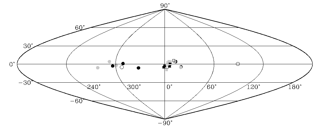
Figure 1: Distribution of the PNe of our sample in the Galactic coordinates. Circles represent objects of the Galactic disk and squares, objects belonging to the Galactic bulge. Filled black symbols are new observed objects whose properties are summarized in Table 1. Gray and white symbols are objects from the literature and are also analysed in this work. They are described in Sect. 4.4.1.

In Fig. 1 we show the location of our sample objects in the Galactic coordinates plane. We have included our new observed objects (black dots) as well as the literature data described in Sect. 4.4.1 (grey and white symbols). The symbols differentiate between bulge (squares) and disc (circles) PNe. This choice will be maintained throughout the paper. We estimated Galactocentric distances, $R_{G}$, for most of the PNe using the statistical distances computed by Stanghellini & Haywood (2010), except for He 2-96, for which we assumed the distance computed by Tajitsu & Tamura (1998). We adopted a Galactocentric distance for the Sun of 8 kpc. Additionally, we also computed the height over the Galactic plane, $z$, using the estimated heliocentric distances and the Galactic latitude for each PNe, trying to identify possible PNe belonging to the thick disc. Assuming that the distance scale of the thin disc is about 350 pc, three objects have high probabilities of being thick disc PNe (He 2-158, M 1-33 and M 1-60). We will briefly discuss this topic in Sect. 6.1. The computed $R_{G}$ and $z$ are shown in Table 1. We checked that the selection of the distance scale does not change significantly the distribution of the objects along the Galactic disc by comparing with the Galactocentric distances obtained using the distance scale by Zhang (1995); although individual Galactocentric distances can change, the global behaviour remains the same. Finally, there is no evidence of binary central stars in our sample.

3 Line fluxes, identifications, and extinction correction

We used the splot routine of the IRAF package to measure the line fluxes. The total flux of each line was measured by integrating between two given limits, over a local continuum estimated by eye. In the cases of line blending we used a multiple Gaussian fitting. Owing to the small area covered by our slit, we could not properly extract a sky spectrum. However, taking into account the wider profiles of the emission lines with respect to the telluric lines, it was easy to distinguish telluric emission features from nebular emission lines. We checked carefully line blendings (especially with telluric emission lines) in our 2D wavelength calibrated spectra. The cases in which nebular emission lines are severely blended with sky emission features were not considered and are not included in our line identification tables (see Tables LABEL:tab:lineid1 to LABEL:tab:lineid9 in the Appendix). Finally, several lines are strongly affected by atmospheric features in absorption, by internal reflections of the optics or by bleeding of the emission from the most brightest lines in adjacent orders, rendering their intensities unreliable. In some cases, where we consider we could deblend the line from the non-nebular emission feature, we decided to report the line flux anyway, and included a label in the line identification table as a note of caution. We have to emphasize that we did not correct for telluric emission/absorptions in the reddest part of the spectra. Although we have labeled in Tables  LABEL:tab:lineid1 to LABEL:tab:lineid9 lines clearly affected by telluric emission/absorptions, we can not discard that other lines at the reddest wavelenghts of our spectra could be slightly affected by narrow telluric absorptions, and these fluxes should be considered with caution.

The four different spectral ranges covered in the spectra have overlapping regions at the edges. To produce a homogeneous data set of line flux ratios, we have followed the same procedure described in García-Rojas et al. (2015). Some lines that were saturated in the long exposures were measured in the short ones and rescaled to the H$\beta$ flux in a similar way.

The final intensity of a given line in the overlapping regions is the average of the values obtained in both spectra. In general there was an excellent agreement between line fluxes measured in overlapping spectra. The differences for each line do not show any systematic trend and, for the brightest lines, are always lower than 10%. The differences found for the faintest lines in the overlapping regions can be larger (up to 50%), but the final adopted errors for each line take into account these uncertainties. Therefore, the final adopted uncertainties are always larger than the differences found between both ranges. However, our final results are not substantially affected by these effects because we have not considered fluxes of faint lines of overlapping regions in our analysis.

4 Physical conditions and abundance determinations

4.1 Electron densities and temperatures

The high-quality of our spectra allowed us to use multiple emission-line ratios to derive physical conditions ($n_{\rm e}$ and $T_{\rm e}$) in our objects. The computations of physical conditions and chemical abundances were carried out with Pyneb $v$1.0.26 (Luridiana et al., 2015). To derive the electron density, $n_{\rm e}$, and the electron temperature, $T_{\rm e}$, we cross-converged the temperature and density derived from two sensitive diagnostic line ratios. The method getCrossTemDen included in Pyneb allows the simultaneous determination of $n_{\rm e}$ and $T_{\rm e}$. This routine makes an initial guess of the $T_{\rm e}$ and then, it calculates iteratively the values of $n_{\rm e}$ and $T_{\rm e}$ until convergence. We have used the same state-of-the-art atomic data set as in García-Rojas et al. (2015) which are summarized in Table 2. Errors in the diagnostics were computed via Monte Carlo simulations. We generate 500 random values for each line intensity using a Gaussian distribution centered in the observed line intensity with a sigma equal to the associated uncertainty. For higher number of Monte Carlo simulations, the errors in the computed quantities remain constant. The computed electron temperatures and densities are presented in Table 3.

Table 2: Atomic data set used for collisionally excited lines.

	Transition	Collision
Ion	Probabilities	Strengths
N+	Froese Fischer & Tachiev (2004)	Tayal (2011)
O+	Froese Fischer & Tachiev (2004)	Kisielius et al. (2009)
O2+	Froese Fischer & Tachiev (2004)	Storey et al. (2014)
	Storey & Zeippen (2000)
Ne2+	Galavís et al. (1997)	McLaughlin & Bell (2000)
Ne3+	Butler & Zeippen (1989)	Giles (1981)
	Bhatia & Kastner (1988)
Ne4+	Galavís et al. (1997)	Dance et al. (2013)
	Bhatia & Doschek (1993)
S+	Podobedova et al. (2009)	Tayal & Zatsarinny (2010)
S2+	Podobedova et al. (2009)	Tayal & Gupta (1999)
Cl+	Mendoza & Zeippen (1983)	Tayal (2004)
Cl2+	Mendoza (1983)	Butler & Zeippen (1989)
Cl3+	Kaufman & Sugar (1986)	Galavís et al. (1995)
	Mendoza & Zeippen (1982a)
	Ellis & Martinson (1984)
Ar2+	Mendoza (1983)	Galavís et al. (1995)
	Kaufman & Sugar (1986)
Ar3+	Mendoza & Zeippen (1982b)	Ramsbottom & Bell (1997)
Ar4+	Mendoza & Zeippen (1982a)	Galavís et al. (1995)
	Kaufman & Sugar (1986)
	LaJohn & Luke (1993)
K3+	Kaufman & Sugar (1986)	Galavís et al. (1995)
	Mendoza (1983)
K4+	Kaufman & Sugar (1986)	Butler et al. (1988)
	Mendoza (1983)
Fe2+	Quinet (1996)	Zhang (1996)
	Johansson et al. (2000)
Fe3+	Froese Fischer et al. (2008)	Zhang & Pradhan (1997)
Fe4+	Nahar et al. (2000)	Ballance et al. (2007)
Fe5+	Chen & Pradhan (2000)	Chen & Pradhan (1999)
Fe6+	Witthoeft & Badnell (2008)	Witthoeft & Badnell (2008)
Kr3+	Biémont & Hansen (1986)	Schoning (1997)

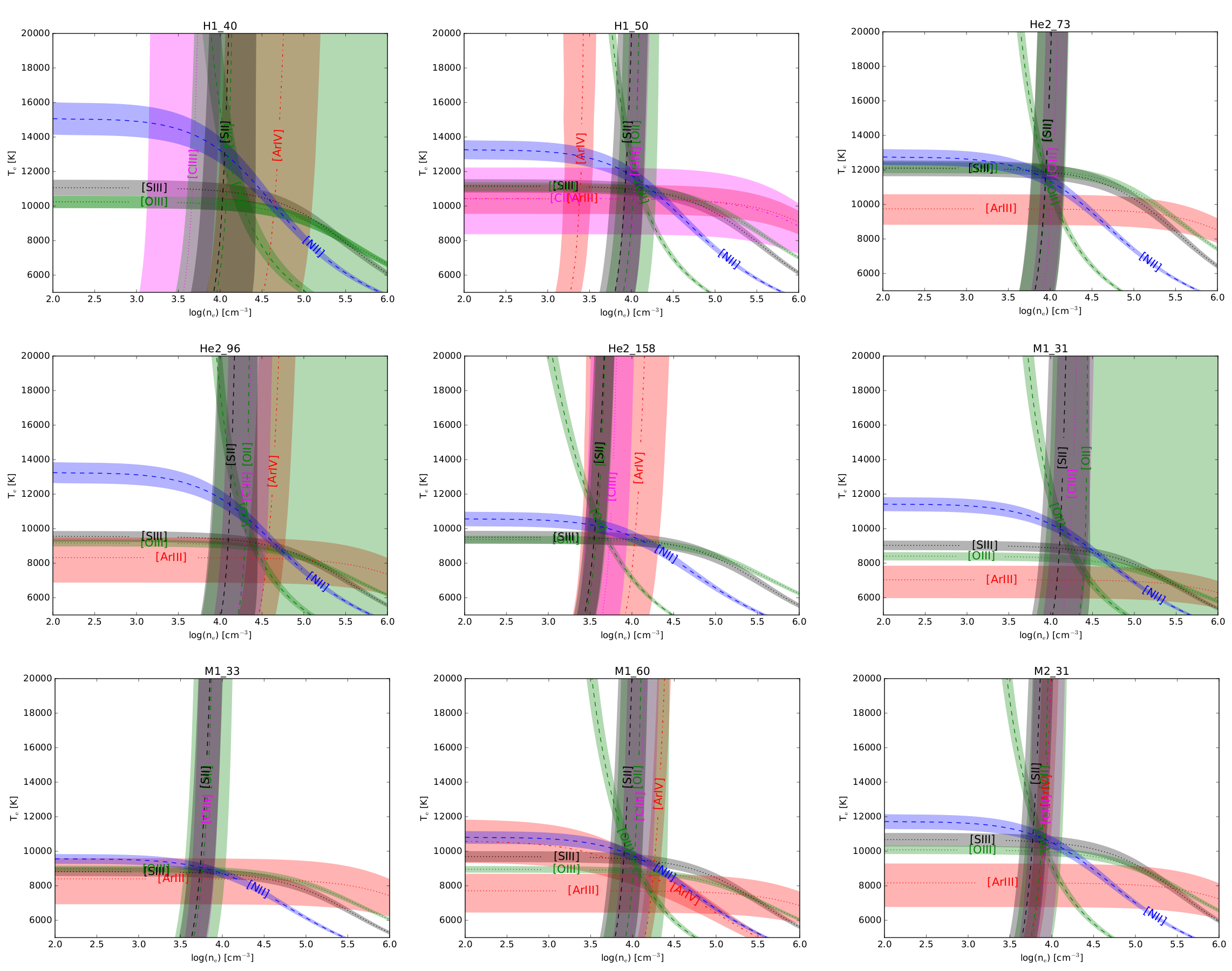
Figure 2: $T_{\rm e}$–$n_{\rm e}$ diagnostic plots. Colors correspond to species: grey for S, blue for N, green for O, magenta for Cl, and red for Ar. Different lines indicate ions: dashed for once ionized ions ([N ii], [O ii] and [S ii]), dotted for two ionized ions ([O iii], [Ar iii], and [Cl iii]), and dotted-dashed for three times ionized ions ([Ar iv]). The width of the coloured bands is related to the uncertainties in the observed line ratios.

We assumed a two-zone ionization scheme. For $n_{\rm e}$, we obtained very similar results from the different diagnostics; therefore, we adopted the average of $n_{\rm e}$([O ii]), $n_{\rm e}$([S ii]), $n_{\rm e}$([Cl iii]) and $n_{\rm e}$([Ar iv]) as representative of the whole nebula for each PN. We adopted the average of electron temperatures obtained from [N ii] and [O ii] lines as representative of the low-ionization zone (IP $<$ 17 eV); we refer to this value as $T_{\rm e}$(low). Similarly, the average of electron temperatures obtained from lines of [O iii], [Ar iii], [S iii], [Cl iv] and [Ar iv] (when available) was assumed as representative of the high-ionization zone (17 eV $<$ IP; $T_{\rm e}$(high), see Table 3). In Fig. 2 we show the diagnostic diagrams computed for our sample objects using Pyneb. This Figure shows the behaviour of the available electron density and temperature diagnostics (also shown in Table 3) in the $T_{e}$ vs. $n_{\rm e}$ plane. Shadowed regions are estimates of the propagated uncertainties in the diagnostics given the observed uncertainties of the line fluxes used in each diagnostic; however, they do not show the effect of the Monte Carlo simulations used to compute the definitive uncertainties and should be taken as orientative only. The final values for $n_{\rm e}$ and $T_{\rm e}$ as well as their computed uncertainties using a Monte Carlo method are those shown in Table 3.

The measured fluxes of the auroral [N ii] $\lambda$5755 line and the trans-auroral [O ii] $\lambda$$\lambda$7320+30 lines have a contribution from recombination. Taking into account these contributions can affect temperature determinations in the low ionization zone and therefore, affect low-ionized species abundance ratios, such as N⁺/H⁺, O⁺/H⁺, Cl⁺/H⁺, and Fe²⁺/H⁺. An estimate of these contributions can be computed using equations 1 and 2 by Liu et al. (2000) led to corrections between 1.7% and 14.6% in the case of the auroral [N ii] $\lambda$5755 line and between 2.8% and 14.8% for the trans-auroral [O ii] $\lambda$$\lambda$7320+30 lines. These values translate into lower temperature determinations: from 80 K to 550 K lower for $T_{\rm e}$([N ii], and from 300 K to 850 K lower for $T_{\rm e}$([O ii]. These corrections are relatively low and the new computed physical conditions and abundances are always within the uncertainties of the previously computed ones. Therefore we have not considered such corrections in our computations. The recombination contribution to the auroral $\lambda$4363 line is negligible for the two objects with the highest excitation in our sample: H 1-50 and He 2-73. We used equation 3 of Liu et al. (2000), where the O³⁺/H⁺ ratio was estimated assuming O³⁺/H⁺=(He/He⁺)^2/3$\times$(O⁺/H⁺+O²⁺/H⁺). Using the values derived for He⁺/H⁺ and He²⁺/H⁺ from optical recombination lines and O⁺/H⁺ and O²⁺ /H⁺ from collisionally excited lines (see Table 4), this contribution amounts to $<$1%, which has almost no effect on the determination of $T_{\rm e}$([O iii]) and therefore, was not considered.

Table 3: Plasma Diagnostic.

Parameter	Line ratio	H 1-40	H 1-50	He 2-73	He 2-96	He 2-158	M 1-31	M 1-33	M 1-60	M 2-31
$n_{\rm e}$ (cm-3)	[O ii] $\lambda$3726/$\lambda$3729	12300${}^{+12250}_{-6100}$	10950${}^{+7250}_{-4350}$	9100${}^{+5000}_{-3200}$	19950${}^{+20500}_{-10000}$	3850${}^{+950}_{-800}$	25300${}^{+21800}_{-11700}$	5900${}^{+3450}_{-2200}$	10550${}^{+9550}_{-5000}$	7650${}^{+4450}_{-2800}$
	[S ii] $\lambda$6731/$\lambda$6716	11150${}^{+5700}_{-3800}$	8900${}^{+3700}_{-2600}$	8900${}^{+3400}_{-2450}$	13000${}^{+9050}_{-5350}$	3650${}^{+900}_{-750}$	13200${}^{+8700}_{-5250}$	5650${}^{+2500}_{-1750}$	8150${}^{+3350}_{-1650}$	6000${}^{+2100}_{-1500}$
	[Cl iii] $\lambda$5538/$\lambda$5518	—a	10800${}^{+3500}_{-2600}$	10550${}^{+4000}_{-2900}$	19350${}^{+19250}_{-9550}$	5500 ${}^{+4250}_{-2400}$	16300${}^{+12050}_{-6950}$	6000${}^{+2100}_{-1550}$	11300${}^{+6600}_{-4150}$	8100${}^{+4500}_{-2850}$
	[Ar iv] $\lambda$4740/$\lambda$4711	—	—	—	37000${}^{+30600}_{-15600}$	10750${}^{+20300}_{-7050}$	—	—	17800${}^{+3600}_{-3000}$	7750${}^{+2000}_{-1600}$
	adopted	11650${}^{\bf+4400}_{\bf-3200}$	10650${}^{\bf+1300}_{\bf-1150}$	9700${}^{\bf+1700}_{\bf-1450}$	19250${}^{\bf+3900}_{\bf-3400}$	3550${}^{\bf+450}_{\bf-400}$	16750${}^{\bf+3850}_{\bf-3150}$	5900${}^{\bf+850}_{\bf-750}$	13500${}^{\bf+1800}_{\bf-1600}$	7250${}^{\bf+950}_{\bf-850}$
$T_{\rm e}$ (K)	[N ii] $\lambda$5755/$\lambda$6548	13350$\pm$1500	12250$\pm$1000	11700$\pm$700	11250$\pm$950	10250$\pm$300	9750$\pm$1100	9600$\pm$300	10200$\pm$500	11250$\pm$500
	[O ii] $\lambda\lambda$3726+29/$\lambda\lambda$7320+30	13450$\pm$2700	13750$\pm$2200	12150$\pm$1900b	—b	—b	9250$\pm$2700	—b	10950$\pm$1900	12000$\pm$1800
	Low	13400$\pm$1100	12250$\pm$650	11750$\pm$500	11250$\pm$950	10250$\pm$300	9700$\pm$800	9600$\pm$300	10200$\pm$400	11250$\pm$400
	[O iii] $\lambda$4363/$\lambda$4959	10140$\pm$350	11000$\pm$250	12000$\pm$300	8950$\pm$300	9300$\pm$200	8250$\pm$250	8950$\pm$150	8850$\pm$200	10000$\pm$250
	[S iii] $\lambda$6312/$\lambda$9069	10950$\pm$450	10950$\pm$350	11850$\pm$450c	9250$\pm$450	9400$\pm$400	8800$\pm$350	8750$\pm$250	9500$\pm$300	10500$\pm$400
	[Ar iii] $\lambda$5192/$\lambda$7135	9700$\pm$750	10400$\pm$800	9700$\pm$900	8300$\pm$1250	—	7000$\pm$950	8400$\pm$1300	7700$\pm$1150	8150$\pm$1200
	[Cl iv] $\lambda$5323/$\lambda$7531	—	10400$\pm$1900	—	—	—	—	—	—	—
	[Ar iv] $\lambda\lambda$7136+7751/$\lambda\lambda$4711+40	—	—	—	—	—	—	—	8500$\pm$850	—
	High	10250$\pm$250	10850$\pm$150	11600$\pm$150	9100 $\pm$200	9350$\pm$100	8500$\pm$150	8850$\pm$100	9100$\pm$100	10150$\pm$150

^a

[Cl iii] $\lambda$5517 line affected by ghost and not considered.

^b

[O ii] $\lambda$$\lambda$7320+30 lines affected by telluric emission lines.

^c

[S iii] $\lambda$9069 line affected by telluric absorption lines. $\lambda$9531 line used instead.

4.2 Ionic abundances from collisionally excited lines

We compute the ionic abundances from multiple ionic CELs of heavy elements. For each ion, we use the same CELs, when available, as those shown in Table 8 of García-Rojas et al. (2015). We did not use auroral or trans-auroral lines to compute abundances owing to their large dependence on the assumed $T_{\rm e}$. We computed abundances using Pyneb (Luridiana et al., 2015) and the atomic data shown in Table 2. Errors in the line fluxes and the physical conditions were propagated via Monte Carlo simulations. For all the objects we used a two-zone scheme of the nebula, adopting a unique $n_{\rm e}$ value in the two zones, $T_{\rm e}$(low) for ions with IP$<$17 eV (i.e. N⁺, O⁺, S⁺ and Fe²⁺), and $T_{\rm e}$(high) for ions with IP$>$17 eV (i.e. O²⁺, Ne²⁺, Ne³⁺, Ne⁴⁺, S²⁺, Cl²⁺, Cl³⁺, Ar²⁺, Ar³⁺, Ar⁴⁺, K³⁺, K⁴⁺, Fe³⁺, Fe⁴⁺, Fe⁵⁺, Fe⁶⁺ and Kr³⁺). Ionic abundances are presented in Table 4.

Table 4: Ionic abundances.

	12 + log(X+i/H+)
Ion	H 1-40	H 1-50	He 2-73	He 2-96	He 2-158	M 1-31	M 1-33	M 1-60	M 2-31
He+	11.10$\pm$0.02	10.98$\pm$0.01	10.96$\pm$0.01	11.08$\pm$0.01	11.04$\pm$0.01	11.18$\pm$0.02	11.12$\pm$0.01	11.12$\pm$0.01	11.05$\pm$0.05
He2+	—	10.03$\pm$0.02	10.30$\pm$0.02	—	—	—	9.15$\pm$0.03	8.93$\pm$0.04	8.56$\pm$0.06
N+	6.78${}^{+0.16}_{-0.09}$	6.89$\pm$0.08	7.26$\pm$0.07	7.07${}^{+0.19}_{-0.09}$	7.32$\pm$0.05	7.56${}^{+0.22}_{-0.12}$	7.50$\pm$0.06	7.58${}^{+0.10}_{-0.06}$	7.04$\pm$0.06
O+	7.17${}^{+0.39}_{-0.21}$	7.34${}^{+0.16}_{-0.12}$	7.54${}^{+0.15}_{-0.22}$	7.63${}^{+0.37}_{-0.19}$	7.89$\pm$0.09	7.88:	7.70$\pm$0.10	7.72${}^{+0.17}_{-0.11}$	7.43${}^{+0.11}_{-0.09}$
O2+	8.48$\pm$0.06	8.63$\pm$0.04	8.51$\pm$0.04	8.63$\pm$0.05	8.35$\pm$0.05	8.70$\pm$0.05	8.73$\pm$0.04	8.71$\pm$0.04	8.57$\pm$0.04
Ne2+	8.01$\pm$0.07	8.11$\pm$0.04	8.03$\pm$0.04	8.14$\pm$0.06	7.76$\pm$0.05	8.28$\pm$0.06	8.34$\pm$0.04	8.31$\pm$0.05	8.08$\pm$0.04
Ne3+	—	8.01$\pm$0.11	8.04$\pm$0.09	—	—	—	—	—	—
Ne4+	—	6.35$\pm$0.06	6.83$\pm$0.06	—	—	—	—	—	—
S+	5.22${}^{+0.30}_{-0.17}$	5.63${}^{+0.12}_{-0.10}$	5.80${}^{+0.12}_{-0.09}$	5.72${}^{+0.28}_{-0.16}$	5.74$\pm$0.06	6.04${}^{+0.30}_{-0.20}$	5.97${}^{+0.09}_{-0.07}$	6.07${}^{+0.12}_{-0.09}$	5.74${}^{+0.09}_{-0.06}$
S2+	6.58$\pm$0.04	6.50$\pm$0.03	6.55$\pm$0.04	6.85$\pm$0.04	6.54$\pm$0.03	6.87$\pm$0.04	6.88$\pm$0.03	6.88$\pm$0.04	6.63$\pm$0.03
Cl+	3.39${}^{+0.17}_{-0.22}$	3.75$\pm$0.10	3.91$\pm$0.06	3.78${}^{+0.11}_{-0.08}$	3.85${}^{+0.16}_{-0.27}$	4.07${}^{+0.13}_{-0.08}$	4.11$\pm$0.06	4.09${}^{+0.08}_{-0.06}$	3.67$\pm$0.08
Cl2+	4.88${}^{+0.16}_{-0.11}$	4.83$\pm$0.04	4.83$\pm$0.05	5.06${}^{+0.10}_{-0.08}$	4.80$\pm$0.07	5.23$\pm$0.08	5.15$\pm$0.04	5.21$\pm$0.05	4.92$\pm$0.05
Cl3+	4.40$\pm$0.07	4.95$\pm$0.03	4.76$\pm$0.03	4.34$\pm$0.04	3.74${}^{+0.14}_{-0.19}$	4.40$\pm$0.04	4.68$\pm$0.03	4.77$\pm$0.03	4.67$\pm$0.03
Ar2+	6.16$\pm$0.04	6.10$\pm$0.03	6.24$\pm$0.03	6.39$\pm$0.04	6.03$\pm$0.03	6.54$\pm$0.04	6.50$\pm$0.03	6.55$\pm$0.03	6.21$\pm$0.03
Ar3+	4.79${}^{+0.23}_{-0.29}$	6.04${}^{+0.07}_{-0.05}$	5.99${}^{+0.07}_{-0.05}$	5.08${}^{+0.09}_{-0.07}$	4.67$\pm$0.10	5.55$\pm$0.14	5.83$\pm$0.05	5.82$\pm$0.05	5.72$\pm$0.04
Ar4+	—	4.91$\pm$0.04	5.18$\pm$0.04	—	—	—	—	—	—
K3+	3.59${}^{+0.18}_{-0.25}$	4.30$\pm$0.06	4.04${}^{+0.05}_{-0.08}$	—	—	—	3.92${}^{+0.14}_{-0.17}$	4.02${}^{+0.11}_{-0.17}$	3.98${}^{+0.09}_{-0.11}$
K4+	—	4.02${}^{+0.13}_{-0.16}$	—	—	—	—	—	—	—
Fe2+	5.71${}^{+0.15}_{-0.10}$	4.40$\pm$0.12	4.65$\pm$0.11	4.19${}^{+0.21}_{-0.16}$	5.14$\pm$0.09	5.01${}^{+0.29}_{-0.18}$	4.92$\pm$0.09	4.69$\pm$0.13	4.49${}^{+0.15}_{-0.20}$
Fe3+	—	—	—	—	—	—	—	—	—
Fe4+	—	4.87$\pm$0.13	5.76$\pm$0.08	—	—	—	—	—	—
Fe5+	—	4.41${}^{+0.17}_{-0.24}$	5.20${}^{+0.08}_{-0.10}$	—	—	—	—	—	—
Fe6+	—	5.08:a	—	—	—	—	—	—	—
Kr3+	—	—	3.47${}^{+0.11}_{-0.14}$	—	—	—	—	—	—

^a

[Fe vii] $\lambda$5158.41 line identification is dubious (see Table LABEL:tab:lineid2).

4.3 Ionic abundances from recombination lines

A large number of He i emission lines were detected in the spectra of all the PNe in our sample. These lines arise mainly from recombination, but some of them can be affected by collisional excitation and self-absorption effects. We use the effective recombination coefficients by Porter et al. (2012, 2013) for He⁺. Both collisional contribution effects and the optical depth in the triplet lines are included in the computations. We determine the He⁺/H⁺ ratio from the three brightest He i emission lines: $\lambda\lambda$4471, 5876, and 6678 using Pyneb. We measure several He ii emission lines in the spectra of H 1-50 and He 2-73, and only the bright He ii $\lambda$4686 line in M 1-33, M 1-60 and M 2-31. Hence, we only use the He ii $\lambda$4686 line to compute the He²⁺/H⁺ ratio. The computation adopts the recombination coefficients computed by Storey & Hummer (1995). The adopted He⁺/H⁺ and He²⁺/H⁺ ratios are presented in Table 4.

We detect several ORLs of different ions of C, N, O and Ne in our spectra. We only compute abundances from O ii and C ii recombination lines as they are crucial for our analysis. Ionic abundances using N ii, N iii, and Ne ii ORLs can be computed following the prescriptions given in García-Rojas et al. (2015). Ne ii ORLs are only detected in H 1-50, M 1-33, and M 1-60 but they are extremely faint (uncertainties are always higher than 40%) and, therefore, abundances obtained from these lines should be treated with caution.

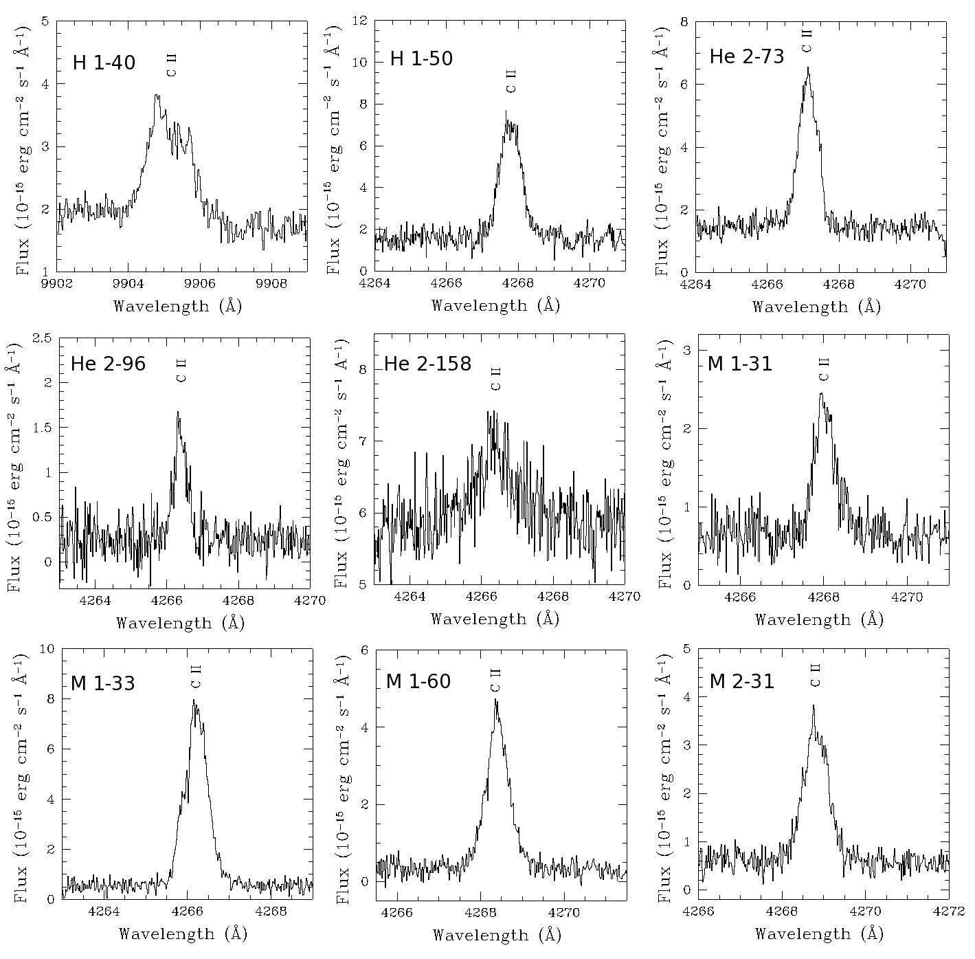
Figure 3: Portion of the spectra showing the brightest C ii recombination line in all the planetary nebulae of our sample (C ii $\lambda$9903 for H 1-40 and C ii $\lambda$4267 for the rest of the objects).

In Fig. 3 we show the brightest C ii recombination line for each PN in our sample. In most of the objects this line is the C ii $\lambda$4267 line, except for H 1-40, where this line was not detected and the brightest one is the C ii $\lambda$9903 line. We compute C²⁺/H⁺ ratios using several C ii lines that, in principle, are excited by pure recombination. We used the recombination coefficients given by Davey et al. (2000). The good agreement between the abundances obtained using the different lines support the recombination origin of these lines. In Table 5 we show the ionic abundances from C ii ORLs.

Table 5: Ionic abundance ratios from the C ii recombination lines^a

Mult.	$\lambda_{0}$	C++/H+ ($\times$10-5)
		H 1-40	H 1-50	He 2-73	He 2-96	He 2-158	M 1-31	M 1-33	M 1-60	M 2-31
6	4267.15	—	34$\pm$5	58$\pm$7	34$\pm$7	20$\pm$4	55$\pm$16	98$\pm$8	82$\pm$9	51$\pm$11
17.06	5342.38	—	—	88:	—	—	—	—	—	—
17.04	6461.95	—	27:	—	43:	—	60$\pm$18	91$\pm$21	81$\pm$26	—
17.02	9903.46	20$\pm$4	34$\pm$8	60$\pm$5	32$\pm$2	—	47$\pm$6	90$\pm$14	76$\pm$7	48$\pm$3
	Adopted	20$\pm$4	34$\pm$4	59$\pm$4	32$\pm$2	20$\pm$4	49$\pm$5	96$\pm$7	78$\pm$5	48$\pm$3

^a

Colons indicate uncertainties higher than 40%. Only lines with intensity uncertainties lower than 40% were considered to compute averaged values (see text).

Figure 4: Portion of the spectra showing the O ii multiplet 1 around 4650 Å in all the planetary nebulae of our sample.

We measure O ii ORLs belonging to multiplet 1 in all the PN of our sample. In Fig. 4 we show the quality of the spectra around this multiplet. We compute O²⁺/H⁺ ratios taking into account departures from local thermodynamic equilibrium (LTE) from the upper levels of the transitions of this multiplet for densities $n_{\rm e}$ $<$ 10⁴ cm⁻³ (Ruiz et al., 2003; Tsamis et al., 2003) and using the recombination coefficients computed by Storey (1994). To account for such effect, we apply the non-LTE corrections estimated by Peimbert et al. (2005), obtaining abundances from individual lines that are in better agreement than when not considering this effect. The abundance using the sum of all lines of the multiplet (see Esteban et al., 1998) is not affected by non-LTE effects and generally agrees with those derived from individual lines. In Table 6 we show the ionic abundances from O ii ORLs. Escalante et al. (2012) found that fluorescense may contribute significantly (up to $\sim$20%) to the intensity of O ii multiplet 1 lines in low-excitation PNe, such as the case of IC 418, but we do not have PNe in our sample with such low ionization degree. Hence, we consider the effect of fluorescense to be negligible in O ii multiplet 1 lines in the PNe of our sample. However, some objects of the literature sample (see Sect. 4.4.1) have similar ionization degree than IC 418 (i.e. M 1-25 and M 1-32) and fluorescense cannot be discarded as a possible excitation mechanism of O ii multiplet 1 lines.

Table 6: Ionic abundance ratios from the O ii recombination lines^a

Mult.	$\lambda_{0}$	O++/H+ ($\times$10-5)
		H 1-40	H 1-50	He 2-73	He 2-96	He 2-158	M 1-31	M 1-33	M 1-60	M 2-31
1b	4638.85	67:	91$\pm$28	64$\pm$22	58$\pm$18	31:	80$\pm$22	131$\pm$23	113$\pm$27	74$\pm$22
	4641.81	55:	91$\pm$31	50$\pm$15	50$\pm$14	23:	95$\pm$46	135$\pm$25	163$\pm$32	92$\pm$12
	4649.14	87$\pm$32	108$\pm$15	87$\pm$12	65$\pm$14	32$\pm$10	112$\pm$25	172$\pm$16	144$\pm$16	101$\pm$21
	4650.84	—	124$\pm$49	67$\pm$35	54$\pm$24	43$\pm$20	77:	136$\pm$20	146$\pm$27	67$\pm$23
	4661.64	112:	97$\pm$20	84$\pm$26	60$\pm$22	28:	123$\pm$43	139$\pm$36	119$\pm$22	99$\pm$23
	4673.73	—	—	104:	—	—	192:	130:	151:	107:
	4676.24	115:	93$\pm$26	82$\pm$34	73$\pm$32	—	116$\pm$45	158$\pm$33	127$\pm$34	85$\pm$37
	4696.14	—	—	—	—	—	—	—	—	—
	Sum	87$\pm$32	101$\pm$23	74$\pm$18	60$\pm$15	36$\pm$12	106$\pm$29	149$\pm$21	141$\pm$22	90$\pm$22

^a

Colons indicate uncertainties higher than 40%. Only lines with intensity uncertainties lower than 40% were considered to compute averaged values (see text).

^b

Corrected for non-LTE effects (see text).

^c

Blended with another line or affected by internal reflections or charge transfer in the CCD.

It is to be noted here that the aim of this paper is not to address the “abundance discrepancy problem” (see e.g. García-Rojas & Esteban, 2007; McNabb et al., 2013, and references therein); some words on this topic, however, should be given here. This problem is well known in nebular physics and consist in the fact that, for a given ion, ORLs provide systematically higher abundances than those obtained using CELs; this difference is generally parametrized by the abundance discrepancy factor (ADF), which is the ratio between ORLs and CELs abundances. Wang & Liu (2007) and Delgado-Inglada & Rodríguez (2014) showed that when computed simultaneously, ADFs given by N, O and C ions show an overall agreement that translates in very similar N/O and C/O when computed from both CELs and ORLs. With this method we avoid the biases discussed by Rola & Stasińska (1994) as we have computed the abundances from high-signal-to-noise optical spectra and used the same type of lines to compute C and O abundances. Additionally, Rola & Stasińska (1994) pointed out that the fluxes of C ii faint recombination lines could be systematically overestimated if the signal to noise is low; this argument does not apply anymore as with the combination of high-sensitive detectors and large aperture telescopes, the C ii and O ii ORLs have been detected with high signal to noise in multiple PNe (see Figs. 3 and  4, and García-Rojas, 2017, and references therein).

4.4 Ionization correction factors and total abundances

To compute total abundances we have to correct for unseen ionization stages. To do this, we adopt a set of ionization correction factors (ICFs). For most elements we adopted the ICFs proposed by D-I14 from a large grid of photoionization models. We checked the validity range of the ICFs, depending on the excitation of each PN. In the majority of the cases, the ICFs can be applied. However, these ICFs are not always appropriate and we have considered alternative computations for particular cases (see below). All the elemental abundances are shown in Table 7.

Following the prescriptions given by D-I14, we consider that the contribution of neutral He to the total abundance when He²⁺ is present is expected to be negligible. In the case of PNe with no He²⁺ we did not try any correction owing to neutral He because the available ICFs introduce a trend with the ionization degree (D-I14). However, all the objects in our sample and in the literature sample (see Sect. 4.4.1) are of relatively high ionization degree, (O²⁺/(O⁺ + O²⁺) $>$ 0.7, except M 1-32 which shows O²⁺/(O⁺ + O²⁺)=0.54. Hence, the correction owing to neutral He proposed by D-I14 should be very small or even negligible.

We compute the total C abundance only from ORLs. Equation 39 of D-I14 proposed an ICF based on C²⁺ and O²⁺ abundances derived from ORLs.

We use the classical scheme N/O = N⁺/O⁺ to compute the N abundance (Peimbert & Torres-Peimbert, 1971). The ICF proposed by D-I14 seems to introduce a trend with the degree of ionization in some nebulae (D-I15) but it is adequate for density-bounded PNe and high-excitation radiation-bounded PNe (Delgado-Inglada et al. in preparation). The fact that we observe the [O i] $\lambda$6300 line in all but one of the PNe in our sample indicates that they are likely radiation-bounded nebulae. The low value of He²⁺/(He⁺ + He²⁺), $<0.2$ in all the PNe, suggests that the PNe are relatively low excitation objects. Therefore, for the subsequent analysis we will adopt the N abundances computed using the classical scheme. These arguments can be extended for the literature sample analysed in Sect. 4.4.1.

To compute the total O abundance from ORLs we take into account the contribution of O⁺ by scaling the O⁺/O²⁺ obtained from CELs and, when He ii lines are detected in the spectrum, the ICF provided by D-I14 to take into account the contribution of O³⁺. To compute the total O/H ratio from CELs we follow the prescriptions given by D-I14.

We detect [Ne iii], [Ne iv], and [Ne v] lines in the spectra of H 1-50 and He 2-73. For these objects, we compute the abundances in two ways: i) by adding the ionic chemical abundances, and (ii) by using the ICF scheme of D-I14. We use the ICFs given by their equations 17 and 20, which give the total Ne abundance when only [Ne iii] lines are observed and when both [Ne iii] and [Ne v] lines are observed, respectively. For the other objects we correct for the unseen ionization stages by using equation 17 of D-I14.

As we detect [Cl ii], [Cl iii] and [Cl iv] lines in all our objects we can calculate Cl abundances by simply adding up the ionic abundances of Cl⁺, Cl⁺⁺ and Cl⁺³ (these total abundances are labeled as Cl^k in Table 7). According to the photoionization models of D-I14, the contribution of higher ionization states of Cl to the total abundance will be lower than 0.07 dex for objects with excitation characteristics like those in our sample. We compare these values with those obtained using equation 32 from D-I14 to correct for unseen Cl higher ionization states (marked as Cl^j in Table 7). There is an excellent agreement between both determinations, indicating that the ICF from equation 32 is working well and that the contribution of higher ionization states is rather small or even inexistent. We also use equation 29 from D-I14, which provides an ICF when only [Cl iii] lines are observed. This equation is valid when O⁺⁺/(O⁺ + O⁺⁺) $>0.02$, which is the case for all the studied PNe. The derived values are represented as Clⁱ in Table 7. The Cl abundances derived with this ICF are, in general, somewhat higher (up to 0.16 dex) than the previous ones. The dispersion shown by the photoionization models around equation 29 is higher than that around equation 32 for the ranges of O⁺⁺/(O⁺ + O⁺⁺) and He⁺⁺/(He⁺ + He⁺⁺) displayed by the PNe studied here (see Fig. 11 and 12 from D-I14), indicating that the ICF from equation 29 provides a more uncertain Cl/H value. Therefore, we choose the Cl abundances labeled as Cl^j,k as the most reliable ones and we use the average between both determinations in the subsequent analysis.

H 1-50 and He 2-73 are the most excited PNe in our sample and we have detected [Ar v] lines in their spectra, besides the [Ar iii] and [Ar iv] lines detected in all our sample of PNe. For these two high excitation PNe, we compute the total Ar abundance as the direct sum of the observed ionization states. As it can be seen from Table 7, the abundances agree (within uncertainties) with those derived using the ICF given by equation 36 of D-I14, which is used when only [Ar iii] lines are observed. For the rest of the objects in the sample, we use this equation to compute the total Ar abundance.

In H 1-50 and He 2-73 we measure several lines of multiple ionization stages of Fe; particularly, and thanks to the high excitation of these PNe we detect relatively bright lines of [Fe v], [Fe vi] and, in H 1-50, [Fe vii]. On the other hand, we measure the most commonly detected [Fe iii] lines in all the PNe in our sample. We use the correction scheme suggested by Rodríguez & Rubin (2005), which is based on the detection of [Fe iii] and an observational fit, given by their equation 3. An alternative approach could be to compute the total Fe abundance by simply adding up all the observed ionic species; however, this approach can only be applied to H 1-50 and He 2-73 and it is quite uncertain as lines from Fe³⁺ were not detected in these objects.

The total Kr abundance in He 2-73 was computed by using equation 3 of Sterling et al. (2015) which accounts for unobserved ions when only [Kr iv] lines are detected.

Table 7: Total abundances of sample A.

	12 + log(X/H)
Ion	H 1-40	H 1-50	He 2-73	He 2-96	He 2-158	M 1-31	M 1-33	M 1-60	M 2-31
He	11.10$\pm$0.02	11.03$\pm$0.01	11.05$\pm$0.01	11.08$\pm$0.02	11.04$\pm$0.01	11.18$\pm$0.02	11.12$\pm$0.01	11.13$\pm$0.01	11.05$\pm$0.01
Ca	8.38${}^{+0.09}_{-0.08}$	8.64$\pm$0.05	8.89$\pm$0.03	8.58$\pm$0.03	8.37${}^{+0.09}_{-0.08}$	8.76${}^{+0.05}_{-0.06}$	9.06$\pm$0.03	8.97$\pm$0.03	8.76$\pm$0.03
Nb	8.10${}^{+0.13}_{-0.18}$	8.20$\pm$0.07	8.27$\pm$0.08	8.09${}^{+0.09}_{-0.10}$	7.91$\pm$0.05	8.44$\pm$0.11	8.54$\pm$0.06	8.59$\pm$0.06	8.19$\pm$0.06
O	8.50$\pm$0.06	8.68$\pm$0.04	8.61$\pm$0.04	8.68${}^{+0.10}_{-0.05}$	8.48$\pm$0.04	8.76${}^{+0.11}_{-0.06}$	8.78$\pm$0.04	8.76$\pm$0.04	8.60$\pm$0.04
Od	8.96$\pm$0.17	9.05$\pm$0.10	8.96${}^{+0.10}_{-0.11}$	8.82${}^{+0.12}_{-0.11}$	8.69${}^{+0.16}_{-0.15}$	9.09${}^{+0.17}_{-0.11}$	9.21$\pm$0.07	9.19$\pm$0.07	8.99$\pm$0.11
Nee	8.18${}^{+0.09}_{-0.07}$	8.13$\pm$0.04	8.10$\pm$0.04	8.38${}^{+0.13}_{-0.07}$	8.16$\pm$0.05	8.55${}^{+0.19}_{-0.09}$	8.41$\pm$0.04	8.41$\pm$0.05	8.15$\pm$0.05
Nef	—	8.15$\pm$0.04	8.12$\pm$0.04	—	—	—	—	—	—
Neg	—	8.37$\pm$0.06	8.37$\pm$0.06	—	—	—	—	—	—
Sh	6.88$\pm$0.08	6.85$\pm$0.04	6.87$\pm$0.04	7.08${}^{+0.06}_{-0.05}$	6.68$\pm$0.03	7.09$\pm$0.06	7.13$\pm$0.04	7.14$\pm$0.05	6.92$\pm$0.04
Cli	5.17${}^{+0.11}_{-0.09}$	5.14$\pm$0.03	5.10$\pm$0.04	5.28${}^{+0.08}_{-0.07}$	4.94$\pm$0.06	5.43$\pm$0.07	5.38$\pm$0.03	5.43$\pm$0.04	5.17$\pm$0.04
Clj	5.01${}^{+0.11}_{-0.09}$	5.20$\pm$0.03	5.13$\pm$0.04	5.15${}^{+0.08}_{-0.07}$	4.88$\pm$0.06	5.31$\pm$0.07	5.30$\pm$0.03	5.37$\pm$0.04	5.12$\pm$0.04
Clk	5.02${}^{+0.11}_{-0.08}$	5.21$\pm$0.03	5.13$\pm$0.03	5.16${}^{+0.14}_{-0.17}$	4.88$\pm$0.05	5.32${}^{+0.09}_{-0.07}$	5.31$\pm$0.03	5.38$\pm$0.04	5.13$\pm$0.04
Arl	6.61${}^{+0.08}_{-0.11}$	6.32$\pm$0.03	6.46$\pm$0.04	6.73${}^{+0.07}_{-0.11}$	6.21$\pm$0.05	6.84${}^{+0.08}_{-0.13}$	6.67$\pm$0.04	6.72$\pm$0.04	6.39$\pm$0.03
Arm	—	6.38$\pm$0.04	6.46$\pm$0.04	—	—	—	—	—	—
Fen	6.32$\pm$0.07	5.01$\pm$0.11	5.15${}^{+0.09}_{-0.11}$	4.71${}^{+0.15}_{-0.16}$	5.51$\pm$0.08	5.46${}^{+0.16}_{-0.14}$	5.43$\pm$0.08	5.19$\pm$0.10	5.04${}^{+0.14}_{-0.16}$
Kro	—	—	3.79${}^{+0.13}_{-0.14}$	—	—	—	—	—	—

^a

From C ii ORLs and the ICF by D-I14.

^b

Classic ICF scheme of N/O$\sim$N⁺/O⁺ (see text).

^d

From O ii ORLs, O⁺/O²⁺ from CELs, and the ICF by D-I14.

^e

ICF from equation 17 of D-I14.

^f

ICF from equation 20 of D-I14.

^g

Sum of Ne²⁺, Ne³⁺ and Ne⁴⁺.

^h

Where He ii lines were not detected, ICF from equation 36 of Kingsburgh & Barlow (1994). Where He ii lines were detected, ICF from equation 26 of D-I14.

ⁱ

ICF from equation 29 of D-I14.

^j

ICF from equation 32 of D-I14.

^k

Sum of Cl⁺, Cl²⁺ and Cl³⁺.

^l

ICF from equation 36 of D-I14.

^m

Sum of Ar²⁺, Ar³⁺ and Ar⁴⁺.

ⁿ

ICF from equation 3 by Rodríguez & Rubin (2005)

^o

ICF from equation 3 by Sterling et al. (2015)

4.4.1 High-quality spectroscopic data from the literature

In order to extend our sample of DC PNe, we have computed (following exactly the same methodology) the elemental abundances for the eight DC PNe present in the sample studied by D-I15: Cn 1-5, H 1-50, M 1-42, M 2-27, M 2-31, MyCn 18, NGC 6439, and NGC 7026, and for the nine DC PNe studied by García-Rojas et al. (2012) and García-Rojas et al. (2013): Cn 1-5, Hb 4, He 2-86, M 1-25, M 1-32, M 1-61, M 3-15, NGC 2867 and PB 8. For simplicity, we will refer to the new PNe reported here as sample A, while sample B and C will be composed by the PNe previously studied by D-I15 and García-Rojas et al., respectively. There are two objects in sample B in common with our sample (H 1-50 and M 2-31) and there is also an object that is in both samples B and C (Cn 1-5). In general, we have found a good agreement between the abundances computed for the different samples (within 0.1 dex), with the exception of Cl/H in M 2-31, where we found a Cl abundance about 0.2 dex higher when using the data from D-I15, and for Ar/H in Cn 1-5, which is more than 0.2 dex lower when using the data from the compilation of D-I15. As the quality of our new observational data (sample A) or the data from sample C are much better than those of sample B, we will not consider H 1-50, M 2-31 and Cn 1-5 from sample B, hereinafter. All the recomputed abundances of samples B and C, as well as some properties of the PNe, such as Galactic component they belong, Galactocentric distances, height over the Galactic plane, and dust type, are presented in Table 8.

Table 8: Abundances recomputed for DC PNe from the literature (samples B and C).

12 + log(X/H)

Gal.

$R_{G}$

$z$

Dust

Ref.

PNe

Comp.

(kpc)a

(pc)a

type

He/H

N/H

O/H

Ne/H

Ar/H

S/H

Cl/H

log(C/O) (RLs)

(Sample)

Cn 1-5

bulge

2.504

$-$920

DCcr

11.10$\pm$0.01

8.72${}^{+0.04}_{-0.05}$

8.78$\pm$0.04

8.62${}^{+0.05}_{-0.04}$

6.82$\pm$0.05

7.15$\pm$0.04

5.47$\pm$0.03

0.08$\pm$0.07

1 (C)

Hb 4

bulge

2.932

260

DCcr

11.05$\pm$0.02

8.93${}^{+0.10}_{-0.11}$

8.66$\pm$0.05

8.12${}^{+0.06}_{-0.05}$

6.58${}^{+0.05}_{-0.07}$

7.12${}^{+0.09}_{-0.10}$

5.28$\pm$0.04

$-$0.29${}^{+0.06}_{-0.05}$

1 (C)

He 2-86

disc

7.139

$-$217

DCam+cr

11.11$\pm$0.02

8.81${}^{+0.09}_{-0.13}$

8.75$\pm$0.04

8.37${}^{+0.06}_{-0.04}$

7.03${}^{+0.06}_{-0.08}$

7.25${}^{+0.08}_{-0.10}$

5.37${}^{+0.05}_{-0.04}$

$-$0.14$\pm$0.03

1 (C)

M 1-25

bulge

2.527

898

DCcr

11.11$\pm$0.02

8.43${}^{+0.06}_{-0.04}$

8.78${}^{+0.09}_{-0.06}$

7.92${}^{+0.13}_{-0.08}$

6.70$\pm$0.05

7.18${}^{+0.07}_{-0.06}$

5.42${}^{+0.05}_{-0.04}$

$-$0.21$\pm$0.08

1 (C)

M 1-32

disc

3.466

354

DCcr

11.10$\pm$0.02

8.46${}^{+0.06}_{-0.05}$

8.53${}^{+0.13}_{-0.09}$

7.82${}^{+0.15}_{-0.11}$

6.54$\pm$0.06

7.16$\pm$0.08

5.30$\pm$0.05

0.39${}^{+0.09}_{-0.11}$

1 (C)

M 1-42

bulge

2.465

$-$472

DCcr

11.23$\pm$0.02

8.70$\pm$0.04

8.47$\pm$0.04

8.04${}^{+0.04}_{-0.05}$

6.46$\pm$0.04

6.93$\pm$0.04

5.23$\pm$0.04

$-$0.24$\pm$0.06

2 (B)

M 1-61

disc

3.433

$-$502

DCam+cr

11.06$\pm$0.02

8.33${}^{+0.11}_{-0.14}$

8.65${}^{+0.06}_{-0.04}$

8.22${}^{+0.07}_{-0.05}$

6.82${}^{+0.06}_{-0.09}$

7.05${}^{+0.10}_{-0.11}$

5.14${}^{+0.05}_{-0.04}$

$-$0.14$\pm$0.06

1 (C)

M 2-27

bulge

4.500

$-$1005

DCcr

11.15${}^{+0.02}_{-0.03}$

8.91$\pm$0.06

8.86$\pm$0.04

8.53$\pm$0.04

6.73$\pm$0.03

7.33${}^{+0.06}_{-0.05}$

5.58${}^{+0.06}_{-0.05}$

$-$0.36${}^{+0.06}_{-0.07}$

3 (B)

M 3-15

bulge

1.480

495

DCcr

11.06$\pm$0.02

8.45${}^{+0.11}_{-0.13}$

8.78${}^{+0.06}_{-0.05}$

8.14$\pm$0.07

6.95$\pm$0.06

7.21${}^{+0.11}_{-0.14}$

5.28$\pm$0.05

$-$0.25$\pm$0.11

1 (C)

MyCn 18

disc

6.528

$-$288

DCam+cr

11.00${}^{+0.02}_{-0.03}$

8.46${}^{+0.06}_{-0.05}$

8.56$\pm$0.04

8.40$\pm$0.04

6.49$\pm$0.04

7.26$\pm$0.06

5.49$\pm$0.04

$-$0.50${}^{+0.05}_{-0.06}$

4 (B)

NGC 2867

disc

7.996

$-$233

DCcr

11.03$\pm$0.01

7.94$\pm$0.05

8.56$\pm$0.04

7.88$\pm$0.04

6.18$\pm$0.04

6.67${}^{+0.06}_{-0.05}$

4.97$\pm$0.03

0.38${}^{+0.05}_{-0.06}$

5 (C)

NGC 6439

bulge

2.130

658

DCcr

11.12$\pm$0.02

8.50${}^{+0.05}_{-0.04}$

8.68$\pm$0.04

8.20$\pm$0.04

6.59$\pm$0.03

7.08${}^{+0.05}_{-0.06}$

5.38$\pm$0.04

$-$0.04${}^{+0.07}_{-0.06}$

3 (B)

NGC 7026

disc

8.232

14

DCcr

11.08$\pm$0.02

8.60${}^{+0.03}_{-0.04}$

8.71$\pm$0.02

8.21$\pm$0.03

6.49$\pm$0.02

7.21$\pm$0.04

5.43$\pm$0.03

$-$0.09${}^{+0.06}_{-0.07}$

6 (B)

PB 8

disc

8.558

536

DCcr

11.09${}^{+0.01}_{-0.02}$

8.25${}^{+0.07}_{-0.08}$

8.75${}^{+0.05}_{-0.04}$

8.25$\pm$0.05

7.08$\pm$0.06

7.29$\pm$0.08

5.63${}^{+0.07}_{-0.08}$

$-$0.39${}^{+0.05}_{-0.06}$

5 (C)

^a

Galactocentric distances computed from heliocentric distances by Stanghellini & Haywood (2010) and using equation given in Table 1. $z$ is the height above the Galactic plane in pc and was computed following equation in Table 1.
References: (1) García-Rojas et al. (2012); García-Rojas et al. (2013); (2) Liu et al. (2001); (3) Wang & Liu (2007); (4) Tsamis et al. (2003); (5) García-Rojas, Peña, & Peimbert (2009); (6) Wesson, Liu, & Barlow (2005)

4.5 Comparison with other abundance determinations in the literature

We have compared our abundance determinations for sample A objects with the recent study made by García-Hernández & Górny (2014) for a large sample of PNe compiled from the literature. All our sample A PNe, with the exception of M 1-33 were studied by García-Hernández & Górny (2014). In general, we find a very good agreement in the He and O abundances in both sets (agreement within 0.04 and 0.1 dex, respectively). The agreement between N abundances is also relatively good (within 0.2 dex); the same occurs for S, Ar, and Ne, except for some objects for which the Ar and Ne abundance differences reach higher than 0.3 dex. We ascribe these differences to the different sets of atomic data and ICFs used by García-Hernández & Górny (2014). In fact, the effects on the abundances of using different atomic data sets have been recently studied by Juan de Dios & Rodríguez (2017); these authors pointed out that for PNe with electron densities higher than 10⁴ cm^-3, the use of different atomic data sets can produce differences in computed abundance ratios such as O/H or N/O of a factor of 4. We have avoided using the atomic data sets that reach to even higher differences, but the abundances of our high-density PNe are likely to be affected by the systematic uncertainties introduced by atomic data. On the other hand, the high quality and signal to noise of our spectra represent a substantial improvement to previous data sets; additionally we have used an up-to-date ICF scheme, which make our abundance determinations more reliable.

C abundances have been previously computed from UV CELs only for 1 object of sample A (H 1–50). Wang & Liu (2007) reported a C/O ratio from UV/optical CELs of 0.15, which was later recomputed by Delgado-Inglada & Rodríguez (2014) as 0.17. These values are much lower than the one obtained in this work: C/O = 0.39, which is almost coincident with the C/O ratio of 0.41 reported by Delgado-Inglada & Rodríguez (2014) from C and O ORLs and assuming C/O$\sim$C²⁺/O²⁺. Delgado-Inglada & Rodríguez (2014) compiled C/O ratios computed from both CELs and ORLs for several PNe in the literature; these authors found an overall agreement between C/O ratios computed from CELs and ORLs, however, they also pointed out some outliers, presenting significant different C/O ratios from CELs and ORLs. In the objects in common with our samples B and C, the computed C/O ratios from CELs and ORLs are somewhat different. The difference (C/O_CELs)$-$(C/O_ORLs) is 0.27, $-$0.20, $-$0.20, and $-$0.17 dex for Cn 1-5, M 1-42, NGC 6439 and NGC 7026, respectively. These differences can be attributed to several effects: i) as PNe are extended objects (at least, more extended than the slit width of optical observations), the volume of the PN covered by optical and UV observations are different and ionization structure effects could be affecting the computed C/O ratios, and ii) UV data are extremely sensitive to uncertainties in the computed extinction.

5 Nucleosynthesis models for low- to intermediate-mass stars

We compare the derived nebular abundances with two state-of-the-art sets of AGB nucleosynthesis models that use different approaches to the calculations. The AGB nucleosynthesis models calculated using the Monash code (Karakas & Lattanzio, 2007) and presented by Karakas & Lugaro (2016, hereinafter KL16) for $Z$ = 0.007, 0.014 and 0.03. The AGB nucleosynthesis models obtained by using the ATON code for stellar evolution (Mazzitelli, 1989; Ventura et al., 1998; Ventura & D’Antona, 2009) presented by Ventura et al. (2013) for $Z$ = 0.008, by Di Criscienzo et al. (2016) for $Z$ = 0.018 and by García-Hernández et al. (2016b) for $Z$ = 0.04. We label this set of models as ATON16. The abundances represented by the models are the final AGB abundances. No extra nucleosynthetic products are expected to be carried into the nebula during the AGB-PN transition. For the sake of simplicity, we will refer to the $Z_{\rm KL16}$=0.007 and $Z_{ATON16}$=0.008 as sub-solar metallicity models, $Z_{\rm KL16}$=0.014 and $Z_{\rm ATON16}$=0.018 as solar metallicity models and $Z_{\rm KL16}$=0.03 and $Z_{\rm ATON16}$=0.04 as super-solar metallicity models. The difference in metallicities between KL16 and ATON16 models comes from the different reference for Solar metallicity adopted by the two groups: KL16 adopt the solar abundances given by Asplund et al. (2009) while the ATON16 models assume solar abundances by Grevesse, Noels, & Sauval (1995). The differences in the assumed input physics between KL16 and ATON16 models come from the mass-loss rate adopted and from the treatment of convection during the AGB evolution. The KL16 models use the Vassiliadis & Wood (1993) mass-loss rate whereas ATON16 models use the Bloecker (1995) mass-loss prescription in the oxygen-rich regime with $\eta_{r}=0.02$ (Ventura et al., 2000). In the ATON16 models during the carbon-rich phase the mass-loss rate based on the hydrodynamical models of carbon stars by Wachter et al. (2002, 2008) is adopted. As for the convection treatment, the ATON16 models differ from those by KL16 in that they use the full spectrum of turbulence (FST) convective model (Canuto & Mazzitelli, 1991) instead of the mixing length theory. The net result is a more efficient HBB and a lower threshold mass for the activation of these processes in the ATON16 models.

Finally, we note that KL16 included a partial mixing zone (PMZ) between the convective H-rich envelope and the intershell at the deepest extent of each TDU in some models; this was done to produce enough ¹³C nuclei in the He intershell, to release neutrons for an efficient production of the elements heavier than iron via slow neutron captures (the $s$-process), as required by the observations (e.g. Busso et al., 2001). All KL16 1.5–4.5 M_⊙ models for sub-solar metallicities, 1.5–4.75 M_⊙ models for solar metallicities and 2.5–4.5 M_⊙ models for super-solar metallicities include a PMZ. However, the presence of the PMZ has almost no effect on the abundances of interest here (it mainly affects the $s$-process elements), with at most an increase of 0.05 dex in the C abundances for models with small or no PMZ. Regarding the initial abundances, KL16 employed the solar abundances from Asplund et al. (2009) for $Z$=0.014 and scaled them by a factor of two up (for $Z$=0.03) or down ($Z$=0.007). In this way the initial elemental ratios are constant (as seen in the following plots). The $Z$ = 0.018 and $Z$ = 0.04 ATON models have a solar-scaled mixture, while an alpha-enhancement $[\alpha/{\rm Fe}]=+0.2$ is used for the $Z$=0.008 models.

6 Comparison between observations and with AGB nucleosynthesis predictions

The accurate abundances that we have obtained for sample A allow us to compare with the predictions of AGB stellar nucleosynthesis models to better constrain the progenitor masses of these objects. As we mentioned before, one of our aims is to understand the simultaneous presence of PAHs and silicates in DC PNe and the role of the progenitor mass in this behaviour.

6.1 Metallicity indicators. Behaviour of chlorine and oxygen abundances in the sample

Chlorine (Cl) is considered a better metallicity tracer for PNe than oxygen as there are observational evidences of O-enrichment in PNe at low-metallicity (see e.g. Peña, Stasińska, & Richer, 2007) and at somewhat lower than solar-metallicity PNe (D-I15). Post-AGB stars in the Magellanic Clouds also show evidence of O-enrichment (e.g., De Smedt et al., 2012). This enrichment has been attributed to the PN progenitor stars having experienced dredge-up of material into the He-rich intershell from the C-O core, where O is present due to production via ¹²C($\alpha$,$\gamma$)¹⁶O during the core He-burning (see e.g. Péquignot et al., 2000). The occurrence of such O dredge-up is supported by low-metallicity AGB theoretical models (Marigo, 2001; Herwig, 2004; Karakas & Lugaro, 2010) and slightly subsolar-metallicity models that include diffusive overshooting (García-Hernández et al., 2016a).

The values of the O/Cl abundance ratios are plotted in Fig. 5 as a function of the Cl and O abundances for all our sample objects. The results are compared with the protosolar values of Lodders (2010) and with the set of Galactic H ii regions (red stars in Fig. 5) studied by Esteban et al. (2015). The most striking feature of Fig. 5 is the apparent anticorrelation between the values of O/Cl and Cl/H, which would indicate that the O abundance varies more slowly than that of Cl as the metallicity increases. However, an anticorrelation between O/Cl and Cl/H might be introduced by errors in the determination of the Cl abundance. The Cl abundances of our sample objects have been calculated in an inhomogeneous way. For the PNe in sample A objects (filled black symbols in Fig. 5), the H ii regions, and for most of the PNe in sample C (grey symbols) the Cl abundances could be computed without applying any ICF correction, but for PB 8 and all the PNe in sample B (open symbols in Fig. 5), the Cl abundances are based on the ICF given by equation 29 of D-I14. D-I15 show in their Fig. 3 that the uncertainties of O/Cl and Cl/H, with the Cl abundances calculated with the ICF of equation 29 of D-I14, are anticorrelated, and can easily lead to an anticorrelation between these two quantities. In order to illustrate the effect of these different approaches, we show with arrows in the upper panel of Fig. 5 the positions that some of the objects would occupy if the ICF of equation 29 of D-I14 had been used to derive their Cl abundances. It is clear from these arrows that most, if not all, of the anticorrelation between O/Cl and Cl/H can be explained by the effects of using an ICF for several objects. Besides, any other uncertainty in the determination of Cl/H that does not affect the calculation of O/H will have a similar effect, moving the points in the direction of the arrows.

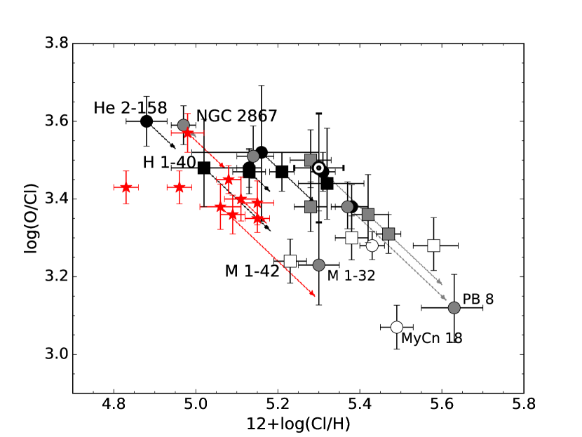
Figure 5: Values of log(O/Cl) vs. 12+log(Cl/H) (upper panel) vs. 12+log(O/H) (lower panel) for our sample of objects. The Cl/H ratio has been computed by simply adding available ionic abundances or by using equation 29 of D-I14 when only [Cl iii] lines were available in the spectra (PNe of sample B and PB 8). The effect of considering using the ICF of equation 29 of D-I14 is shown by arrows. Filled black symbols are the PNe of our sample (sample A); open symbols are DC PNe from D-I15 (sample B) and filled grey symbols are those studied by García-Rojas et al. (2013, sample C). Squares are bulge PNe and circles are disc PNe. Red stars represent H ii region abundances from the sample of Esteban et al. (2015). The protosolar abundances of Lodders (2010) are overplotted with the solar symbol.

Our values of O/H are not affected by as many inhomogeneities or uncertainties as those plaguing our determinations of Cl/H, as can be seen by the lack of correlation between the values of O/Cl and O/H shown in the lower panel of Fig. 5. Furthermore, as we show in Fig. 6, the stellar nucleosynthesis models that predict the largest variations in O/H do not seem to be representative of the PNe in our sample. Hence, for our objects O/H seems to be a better estimate than Cl/H of the initial metallicity of the progenitor stars. Taking O/H as our metallicity indicator, our PNe are the descendants of stars with metallicities from solar to half-solar.

It is also noticeable from Fig. 5 that there is a significant number of PNe with higher O/H than the H ii regions. This would not be surprising if those PNe belong to the bulge, which has a higher metallicity population, but several of the disc PNe also show higher O/H ratios than those of H ii regions. D-I15 found also that several Galactic disc PNe showed higher Cl, O, Ne, and Ar abundances than Galactic H ii regions. Since these PNe are located between 6 and 9 kpc they can be considered solar neighborhood members, and gradient effects are excluded. D-I15 propose alternative explanations such as stellar migration of central stars, as it is well known to be required to interpret the spread in the age-metallicity relationship in the Galaxy (e.g., see Spitoni et al., 2015) or changes in the stellar composition arising during star formation or stellar evolution.

In Fig. 6 we show the O/Cl ratios as a function of the O/H abundance ratio. We have overplotted the two sets of stellar evolution models with different metallicities. In the KL16 models, the oxygen abundance decreases with progenitor mass due to oxygen destruction via HBB, whereas the ATON16 models show both oxygen production and destruction. The metallicities of around solar and half-solar from the models of KL16 and ATON16 seem appropriate to cover all the metallicity range covered by our PNe, but we also include some higher metallicity models for completeness.

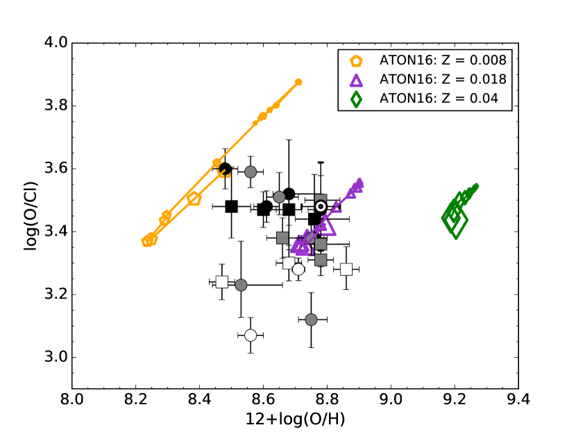
Figure 6: Values of log(O/Cl) vs. 12+log(O/H) for our sample of objects compared with the predictions from the stellar nucleosynthesis models by Karakas & Lugaro (2016) (K16, upper panel) and García-Hernández et al. (2016b) (ATON16, lower panel) for different metallicities. PN symbols are identified in Fig. 5. The protosolar abundances of Lodders (2010) are overplotted with the solar symbol. The symbol sizes relate to the progenitor mass in the models.

6.2 The alpha-elements: Ne, S and Ar abundances

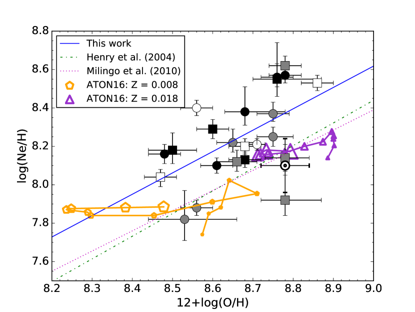
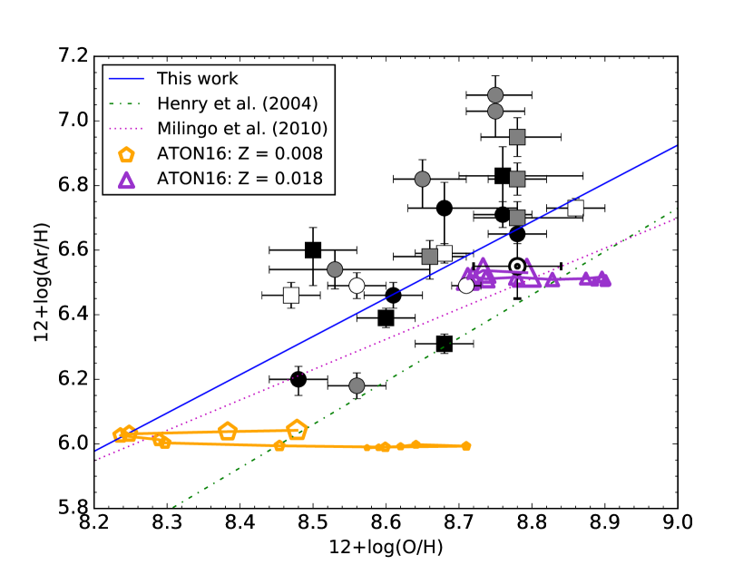
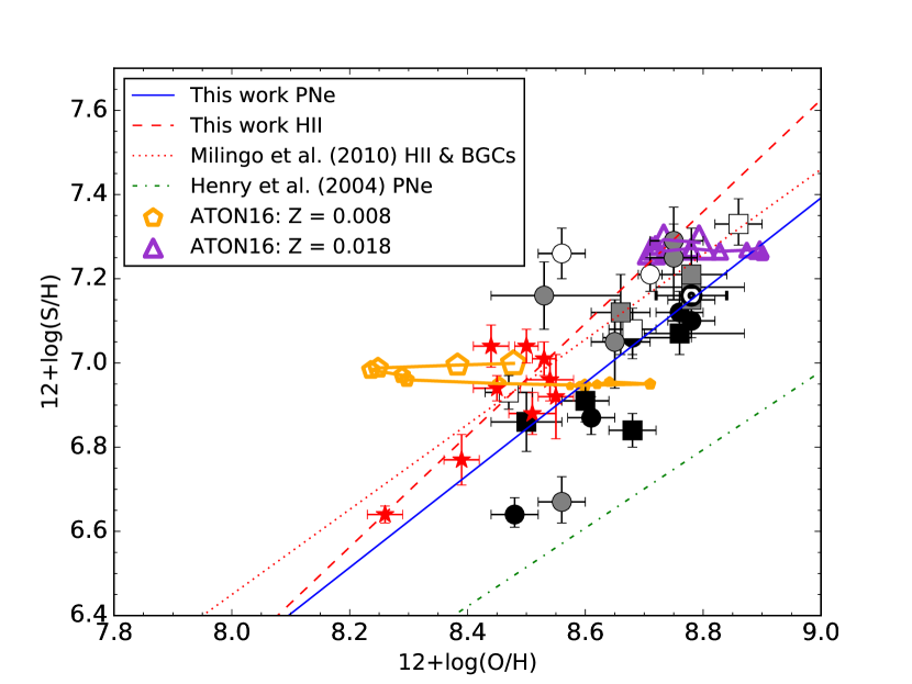
Figure 7: Values of 12+log(Ne/H) (upper panel) and 12+log(Ar/H) (middle panel) and 12+log(S/H) (lower panel) vs. 12+log(O/H) for our sample of objects. Symbols for observations are the same than in Fig. 6. The protosolar abundances of Lodders (2010) are overplotted with the solar symbol. Fits to the observed relations in PNe are shown as continuous blue lines in each panel. Nucleosynthesis ATON16 models for Z= 0.008, 0.018 are also included for comparison (see text).

We have also computed the abundance of other $\alpha$-elements, such as Ne, S and Ar, that are supposed to evolve in lock-step during the chemical evolution of galaxies and hence, a correlation is expected between their abundances and O abundance. In Fig. 7 we show the behaviour of Ne/H vs. O/H (upper panel), Ar/H vs. O/H (middle panel) and S/H vs. O/H (lower panel). A correlation between (Ne, Ar, S) abundances and O abundances is found, as expected. The fits to our data are shown as a continuous blue line on each panel. However, there is a large dispersion in all the relations, which is mainly due to uncertainties in the adopted ICFs. In the upper and middle panel of Fig. 7 we include the fits obtained to the Ne/H vs. O/H and Ar/H vs. O/H relations by Henry, Kwitter, & Balick (2004, green dotted-dashed line) and Milingo et al. (2010, dotted magenta line) from large samples of Galactic PNe. It is clear that the slopes are very similar although the new ICFs by D-I14 used here seem to provide somewhat higher abundances in average ($\sim$0.2 dex) for both Ne and Ar.

It is interesting to note that when comparing to nucleosynthesis ATON16 models Ne/H and Ar/H seem to be overestimated. However, the ICFs for these two elements from optical data have large uncertainties (see discussion in D-I14). KL16 models behave very similarly to ATON16 models in these plots; however, we avoid to show them to not overload Fig. 7.

Furthermore, we can also check the puzzling behaviour of S abundances in our DC PNe sample. Henry, Kwitter, & Balick (2004) coined the expression “sulphur anomaly” to define the phenomenon consisting on the fact that, for a given O/H value, the S/H ratios computed for PNe are systematically lower than those computed for H ii regions in a given galaxy; PNe with C-rich dust features seem to be, on average, more depleted in S than other types of PNe (see e.g. García-Hernández & Górny, 2014). This behaviour has been found for PNe in the Milky Way (see e.g. Henry et al., 2012; Milingo et al., 2010) and in nearby galaxies (Bernard-Salas et al., 2008; Shaw et al., 2010; García-Rojas et al., 2016). Sulphur depletion into dust and sulphur destruction by nucleosynthetic processes during stellar evolution have been proposed to explain this anomaly, but the theoretical models have failed to reproduce the amount of missing sulphur (see Henry et al., 2012; Shingles & Karakas, 2013, and references therein). Henry, Kwitter, & Balick (2004) proposed a failure in the proposed ionization correction schemes to account for the highly ionized S³⁺ state; infrared observations of the [S iv] 10.5 $\mu$m line significantly reduce the sulphur deficit but they cannot completely resolve the anomaly (Bernard-Salas et al., 2008; Henry et al., 2012). This seems to indicate that the contribution from S³⁺ and probably from other ionization stages are commonly underestimated in ICFs computed from photoionization models grids. On the other hand, Badnell et al. (2015) computed revised dielectronic recombination rates that lead to a higher fraction of S⁺ in the gas with respect to S²⁺; unfortunately, these authors claim that this new computations are not enough to solve the “sulphur anomaly”.

In the S/H vs. O/H plot (lower panel of Fig. 7) we plot the fit to our PNe data (solid blue line) together with the fit to our H ii regions data (dashed red line). For comparison, we include also the fit to a large sample of Galactic PNe data by Henry, Kwitter, & Balick (2004) (dotted-dashed green line) and the fit computed by Milingo et al. (2010) to a large sample of H ii regions and Blue Compact Dwarf (BCD) galaxies (dotted red line). Besides the relatively low metallicity coverage of our sample, it seems that the use of the newly computed ICFs by D-I14 improves the situation but does not solve the problem. However, García-Hernández & Górny (2014) found from their analysis of a large sample of PNe with different dust-types, that DC PNe showed the highest S abundances, and that C-rich dust disc PNe seem to show a higher degree of S depletion. This agrees with the hypothesis that S is more depleted into dust grains in the C-rich dust objects, which is supported by the detection of the broad 30 $\mu$m feature in C-rich AGB, post-AGBs and PNe and that is commonly attributed to sulphur-based dust like MgS (e.g. Hony et al., 2002); although a definitive identification is still under debate (see e.g. Zhang et al., 2009; García-Hernández, 2012, and references therein). A recomputation of the ICF of sulphur using the approach of D-I14 and the new dielectronic recombination rates by Badnell et al. (2015), as well as a detailed comparison with high-quality observations of a large sample of PNe covering the different dust-types, would be interesting to see if we are getting closer to resolve the “sulphur anomaly”. Additionally, from Fig. 7 it is clear that ATON16 nucleosynthesis models (and also KL16 ones) reproduce much better the S abundances obtained for our PNe than abundances obtained by Henry, Kwitter, & Balick (2004).

6.3 Nucleosynthesis indicators. Behaviour of nitrogen, helium and carbon abundances

Fig. 8 shows the values of N/O as a function of He/H (upper panel) and C/O (lower panel) for the full sample of DC PNe. The predictions from the nucleosynthesis models by KL16 (left panels) and from ATON models (right panels) are also plotted for sub-solar, solar and super-solar metallicities. As we mentioned in Section 1, the observed abundances of N, He and C in PNe may be significantly affected by the previous occurrence of nucleosynthesis processes, depending on the initial mass and metallicity. We briefly describe here the main behaviour of the AGB models as a function of the progenitor mass and metallicity, in terms of the N/O, C/O and He/H ratios. We also compare the predictions from the nucleosynthesis models with the abundance ratios derived for the three samples (A, B and C) of DC PNe.

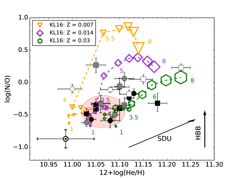
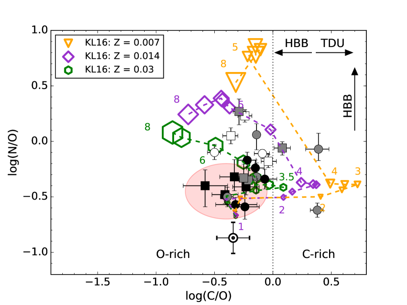
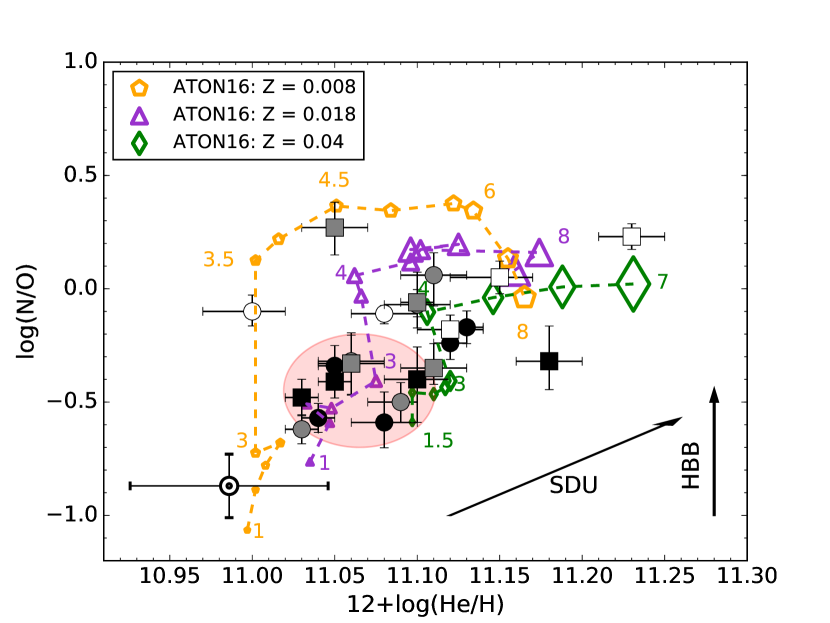
Figure 8: Values of log(N/O) vs. 12+log(He/H) (upper panel) and log(N/O) vs. log(C/O) (lower panel) for our sample of objects compared with the predictions from the stellar nucleosynthesis models by Karakas & Lugaro (2016) (KL16, left panels) and from the ATON stellar nucleosynthesis models (ATON16, right panels) for different metallicities (see text). The size of the model symbols increases with the mass. We have included some mass labels and connected consecutive models with a dashed line to ease interpretation. Symbols for observations are the same than in Fig. 6. Red-shadowed region points to the PNe compatible with having a low-mass (M$<$1.5 M_⊙) progenitor (see text). Arrows indicate what would be the action of the second dredge up (SDU), third dredge up (TDU) and hot bottom burning (HBB) in the represented abundances. The protosolar abundances of Lodders (2010) are overplotted with the solar symbol.

The enhancement in the N/O ratio is, in principle, a clear sign of hydrogen burning. The source of such hydrogen burning is unknown but is inferred to be HBB nucleosynthesis that is active in the more massive AGB stars ($>$3–4 M_⊙, depending on the description adopted for the convective instabilities). The HBB efficiency increases with decreasing metallicity. In the KL16 models, the combined effect of the TDU that increases the surface carbon and the HBB, which converts the dredge-up carbon into nitrogen, produces higher N/O ratios compared to the ATON16 models, because the latter ones experience a less extended TDU. In the low mass regime ($\leq$3 M_⊙), the N/O ratio slightly increases as a function of the initial mass. This is a result of the first dredge-up that brings to the surface the products of the CNO nucleosynthesis, thus N-rich material. Moreover, extra-mixing in low-mass stars (M$<$2 M_⊙) and rotationally induced mixing on the main sequence can also raise the N/O ratio (Karakas & Lattanzio, 2014).

According to the N/O predictions from KL16 and ATON16 models, the progenitor stars of most of the PNe in sample A (filled black symbols) have not gone through any significant HBB, indicating initial masses below $\sim$3–4 M_⊙. The PNe from sample B (empty symbols) exhibit, on average, larger N/O ratios and He abundances, which suggests more massive progenitors (see also García-Hernández et al., 2016b). As for sample C, while some PNe show large N/O ratios, none of them exhibit He-enrichment. The observed behaviour of the whole sample in the N/O vs. He/H diagram agrees better with the high metallicity models (those with solar or super-solar metallicities).

The TDU is responsible for a large enhancement in the surface carbon abundance of some AGB stars. Low-mass stars, with M $<1.5$ M_⊙ (at Solar metallicity, but at slightly lower mass for lower metallicities), do not suffer the TDU and thus preserve C/O$<1$ during their entire life. The strength and the number of dredge-up episodes, together with the initial metallicity, define the final C/O ratio in the stellar surface. For example, solar and super-solar metallicity stars, which formed with a higher O, hardly become carbon stars. The ignition of HBB is evident in the most massive AGB stars where carbon is strongly depleted, in particular in the ATON models. Eventually, final episodes of TDU can be responsible for a final increase in the carbon abundances during the last thermal pulses. Nucleosynthesis models predict that there is a relatively narrow mass range, starting in the limit mass for HBB activation, where the HBB and TDU mechanisms can co-exist and the final stellar surface abundances will depend on which mechanism dominates.

From the log(N/O) vs. log(C/O) panels in Fig. 8, it is clear that most of the PNe have C/O$<1$, which according to model predictions suggest progenitor stars with: 1) M $<1.5$ M_⊙, that have not experienced the TDU and HBB or 2) M $>$ 3–4 M_⊙, that have undergone both the TDU and the HBB, showing the lowest C/O values. Taking into account that Initial Mass Function predicts a larger portion of progenitor stars being low-mass stars, we consider the former channel is more probable, although with the available data, we cannot discard the high-mass channel. Only three PNe from sample C have C/O$>1$: Cn 1–5, M 1-32 and NGC 2867, being the last two PNe extremely C enriched (C/O$>2$).

As for helium abundances, all the PNe present a clear He enrichment relative to the Solar value. He is enhanced by the second dredge-up experienced by stars with M $\gtrsim$ 4M_⊙. The efficiency of this process depends on the H-exhausted core mass of the star and on treatment of convection. The helium abundances predicted by the two set of stellar nucleosynthesis models are similar. The observed values of He/H run over the whole range of He/H predictions, making a difficult task to constrain the progenitor masses of the PNe. However, the highest He abundances (12+log(He/H) $\geq$ 11.15) found for M 2-27 and M 1-42, can be explained by a massive progenitor star formed in a super-solar metallicity environment ($Z$ = 0.03); although only M 2-27 has such a large metallicity (see Table 8).

In summary, we conclude that it is very difficult to reconcile consistently the interpretations on a one-by-one object basis (in terms of progenitor mass and metallicity) from the observations$-$predictions comparison on the N/O. vs. He/H panel with those in the N/O vs. C/O panel, and we must seek alternative explanations (see Sect. 7.1).

7 Discussion

Regarding the N/O vs. C/O behaviour, our sample show most PNe having C/O $<1$ and hence, their ionized gas is “now” oxygen-rich. This behaviour can be explained via two different scenarios: i) the progenitor stars are low-mass stars (M $\lesssim$ 1.5 M_⊙ at solar metallicity but slightly lower for sub-solar metallicity) that have not gone through the TDU, and they remain O-rich during their whole life. In this case the PNe should show , in principle, no enrichment of C, N and He. This applies for some of the PNe of our sample, which simultaneously show low C/O, N/O and He/H. Curiously, most of these PNe, red-shadowed in Fig. 8, display also low Cl/H (or sub-solar metallicities) suggestive of relatively old and low-mass stars. The abundances for three PNe of sample A (M 1-31, M 1-33 and M 1-60, the most metal-rich PNe in sample A) and the whole sample by D-I15 (also more metal-rich objects, on average) seem to disagree with this scenario, mainly due to their high He/H and/or N/O ratios (see below); or ii) the progenitor stars are intermediate-mass stars (M$>$3–4 M_⊙) that have gone through HBB and possibly some TDU events. They end up their evolution as O-rich stars, because HBB destroys the surface C. Their final chemical composition is expected to show up a significant enrichment of N and, depending on the initial mass, some enrichment in He. As it can be seen from Fig. 8 both scenarios fail to explain simultaneously the N/O, He/H and C/O ratios observed. However, this second scenario would be plausible if the progenitor stars have experienced some He pre-enrichment, as Karakas (2014) proposed for bulge PNe in order to explain the paucity of C stars in high-metallicity environments. In Sect. 7.1 we will go further on this. Interestingly, the addition of our accurate C/O ratios into the observations$-$models comparison for a larger sample of DC PNe reveal for the first time that DC PNe may be formed via different channels (e.g., very low-mass objects or more massive HBB stars). García-Hernández & Górny (2014) only compared the median He, N, O and Ar nebular abundances (as obtained from low-resolution optical spectroscopy) observed in a larger number of compact Galactic (both bulge and disc) DC PNe from Stanghellini et al. (2012) (i.e., similar to our sample A) with the older Karakas (2010) AGB nucleosynthesis models, finding that they were consistent with relatively massive ($\sim$3$-$5 M_⊙) and high-metallicity (solar/supersolar) HBB-AGB stars as progenitors; sub-solar metallicity DC PNe are also present in their sample but they do not dominate their median chemical abundance pattern of Galactic DC PNe. On the other hand, García-Hernández et al. (2016b) reached a similar conclusion (i.e., DC PNe mostly descend from high-mass solar/supersolar metallicity HBB-AGBs) by comparing the D-I15 He, N, O and Cl nebular abundances from sample B DC PNe with the ATON16 model predictions; they could not discard, however, another possible formation channels in lower mass AGB stars (like extra mixing, stellar rotation, binary interaction, or even He pre-enrichment) until more accurate C/O ratios would be obtained.

The new DC PNe (sample A) presented here thus suggest the low-mass channel for the first time. This interpretation is similar for both sets of the most recent nucleosynthesis models (KL16 and ATON16); although the exact progenitor masses are somewhat model-dependent. As we already mentioned before, our sample A DC PNe is biased towards compact ($<$4^′′ in diameter, with the exception of H 1-50 and M 1-60 which are 10^′′ in diameter) and (presumably) young PNe but, accidentally, it is mostly composed (6/9) by sub-solar metallicity objects with no significant He and N enrichment. This kind of objects do not dominate the bulk of compact and presumably young DC PNe previously studied by García-Hernández & Górny (2014) neither the DC PNe samples B and C previously studied in the literature (García-Rojas et al., 2013; Delgado-Inglada et al., 2015; García-Hernández et al., 2016b). In principle, both sample B and C objects are also relatively compact. However they are generally more extended than the ones in sample A. All of them with the exception of NGC 2867 (sample B, 14^′′ diameter) and M 1-42 and NGC 7026 (sample C, 9^′′ and 14^′′ diameter respectively) have optical diameters below 7.6^′′ (Acker et al., 1992). On the other hand, sample B objects belong to a sample of relatively early-[WC] type stars, which have, in general, $T_{eff}$ around 50–60 kK (see García-Rojas, Peña, & Peimbert, 2009; García-Rojas et al., 2012, and references therein), with the exception of Hb 4 and NGC 2867 which have central stars with $T_{eff}$ of 86 kK (Tylenda & Stasińska, 1994) and 150 kK (Keller et al., 2014) respectively . The slower evolution of low-mass stars (most of sample A DC PNe) could favor the detection of these objects in very early PN phases (young), while the more massive sources (the ones with the hottest central stars of sample B), evolving faster and even more obscured in the optical, should be more easily detected at later PN phases.

Regarding the dual-dust chemistry phenomenon, the lack of pure C-rich PNe (those with C/O$>$1 and carbon-rich dust) in our sample seem to discard the hypothesis of a late thermal pulse as a main channel to produce the dual-dust features by converting the central stars from O-rich to C-rich (see Perea-Calderón et al., 2009), but it still work for the C-rich DC PNe (C/O$>$1 and mixed chemistry dust) because with the late thermal pulse channel we really would expect such behaviour (i. e, C/O slightly above 1). Therefore, it seems that in both the two hypotheses stated above (low-mass progenitor star or soft HBB stars) the PAHs should have been formed through the dissociation of CO molecule, as proposed by Guzman-Ramirez et al. (2011) (already discussed by García-Hernández & Górny, 2014). However, the scenario proposed by Guzman-Ramirez et al. (2011) assume the presence of a dense toroidal structure, which is prevalent in PNe with binary central stars (Miszalski et al., 2009) and has been also proposed as a result of the ejection of a common-envelope (Passy et al., 2012). Moreover, very recently, Sowicka et al. (2017) have reported the discovery of a binary central star in the DC PN IC 4776 and therefore, this scenario should be taken into account in the future.

7.1 Helium pre-enriched models

As we have commented in the previous section, nucleosynthesis models can not reproduce the observed behaviour of N/O, He/H and C/O simultaneously for the entire sample. Some of these objects belong to the bulge of the Galaxy with a higher metallicity component according to the Cl measurements (M 1-42, M 2-27 from sample B and M 1-31 from sample A). The models presented by Karakas (2014) consider the AGB evolution of stars from the canonical value to helium-enriched compositions at solar and super-solar metallicities. Higher-helium stars evolve at higher luminosities, thus loose the envelope faster and experience a smaller number of TDU events. Furthermore, a higher helium favors a higher entropy barrier at the hydrogen/helium interface, which diminishes the efficiency of TDU. These results in the inhibition of carbon star production which can explain the paucity of C-rich stars in high-metallicity environments. For the moment a grid of models that cover a wide range of masses is not available yet, but for some of them the detailed stellar nucleosynthesis have been calculated. In Figure 9 we present the final abundances for M = 2.5 M_⊙ at solar metallicity and for M = 3.5 and 4.0 M_⊙ for super-solar metallicity. For solar metallicities the initial He abundances adopted were: Y=0.26, 0.28, 0.30, 0,35 and 0.4; for super-solar metallicity models, the initial He abundances were: Y=0.30, 0.32, 0.32 and 0.35 for M = 3.5M_⊙, and Y=0.30, 0.32, 0.35 and 0.4 for M = 4.0 M_⊙. These models have not experienced the HBB and limited episodes of TDU. This is in nice agreement with the objects that have C/O$<1$ and with log(N/O)$<-0.2$ dex, simultaneously, indicating 2.5–4 M_⊙ as possible progenitors of these PNe. The large helium abundances detected would be compatible with a very massive progenitor, with M$\sim$7–8 M_⊙, that experienced deep SDU. This interpretation is however at odds with the measured C/O, which is far in excess than expected. This evidence shifts the attention towards He-rich, lower-mass progenitors, with M$\sim$4–5 M_⊙, which are exposed to a weaker nucleosynthesis at the base of the envelope, compared to their higher mass counterparts. To test this possibility, we calculated a helium-enriched (initial helium Y=0.35) model, with initial mass 4.5 M_⊙. It has been calculated with the ATON code until the very final AGB phases and the correspondent final abundances are shown with orange triangle in the two panels of Figure 9. The results indicate that after the latest thermal pulses, when HBB is turned off, a few TDU events can raise the surface carbon (hence, the C/O ratio significantly) to the observed values. Note that because the mass of the envelope at this stage is significantly reduced, the increase in the surface carbon associated to these late events does not require deep TDU. A wider grid of models would be extremely helpful to better explore this interpretation.

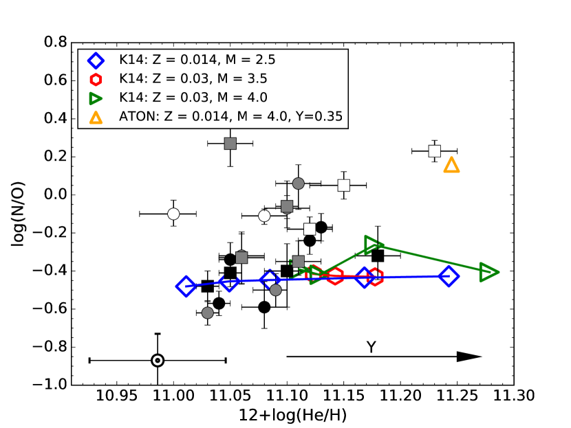
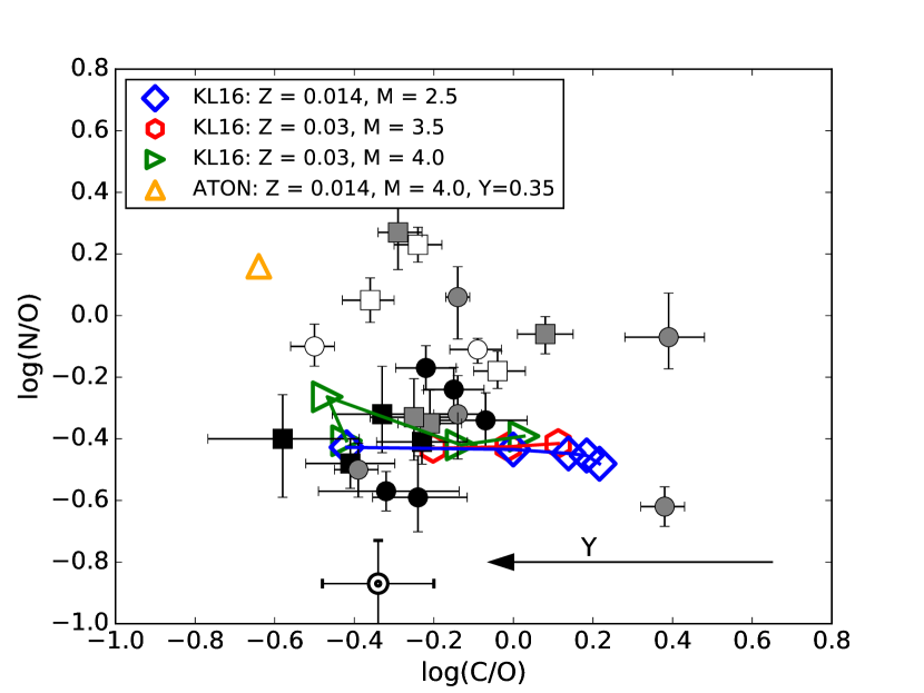
Figure 9: Comparison with helium enriched stellar nucleosynthesis models by Karakas (2014). The arrow show the increasing direction of Y. For solar metallicity models Y=0.26, 0.28, 0.30, 0,35 and 0.4; for super-solar metallicity models Y=0.30, 0.32, 0.32 and 0.35 for M = 3.5M_⊙, and Y=0.30, 0.32, 0.35 and 0.49 for M = 4.0M_⊙.

8 Conclusions

We present deep high-resolution spectrophotometry of nine compact PNe obtained with UVES at the VLT. PNe were selected from the sample of Galactic disc and bulge PNe with dual dust features (cristalline or amorphous silicates + PAHs) detected in their infrared spectra presented by Stanghellini et al. (2012).

We computed physical conditions from a large number of diagnostics, and hence, taking advantage of the large number of emission lines measured in the spectra, computed ionic chemical abundances for a large number of ions from both collisionally excited lines (CELs) and optical recombination lines (ORLs). The total abundances were computed mainly with the ICFs derived by D-I14 but alternative ICFs were considered in a few cases (N and Fe). In particular we take advantage of the quality of our spectra to compute C/O ratios using ORLs.

We extend the initial sample (Sample A) with seven PNe studied by D-I15 and nine by García-Rojas et al. (2012); García-Rojas et al. (2013). These two new samples are refered to as Sample B and Sample C, respectively. The abundances of these PNe were re-computed following the same procedure as for Sample A.

Although Cl has been recently invoked as a better proxy for metallicity for C-rich dust PNe, from the comparison of O/Cl abundance ratios $vs.$ Cl/H and O/H ratios, we reach to the conclusion that O is a better metallicity tracer than Cl for our sample, owing to the inhomogeneities or uncertainties involved in our determinations of Cl/H. From the comparison with nucleosynthesis models, it seems that metallicities around solar and half-solar covers all the metallicity range in the PNe in our sample.

We studied the abundances of Ne, S, and Ar because these elements are expected to evolve in lockstep and we compared them with the O abundances, that can be slightly affected by nucleosynthesis. The abundances derived here define a similar trend between Ne/H, S/H, Ar/H and O/H than the ones previously obtained in the literature (Henry, Kwitter, & Balick, 2004; Milingo et al., 2010) but our abundances are somewhat higher (likely due to the use of different ICFs).

The abundances of N, C, and He derived for the PNe were used to study nucleosynthesis occurring in the progenitor stars. Many of the PNe from sample B have higher N/O values than the other PNe, suggesting that many of the progenitors of Sample B PNe have masses above 3–4 M_⊙. Most of the PNe (with the exception of Cn 1.5, M 1-32, and NGC 2867) have $-$0.5 $<$ C/O $<1$ which can be explained with progenitors with masses i) below 1.5 M_⊙, that have not gone through the TDU, or ii) above 3–4 M_⊙, that have experienced TDU and HBB. All the PNe show some He enrichment, where M 2-27 and M 1-42 are the most extreme in our sample and therefore, likely arise from more massive progenitors.

The values of C/O in the PNe reflect the present dominant chemistry (either oxygen- or carbon-rich) in the gas. As we mentioned before, since all but three PNe have C/O $<1$, the hypothesis of the last thermal pulse that turns O-rich PNe into C-rich PNe is discarded (with the exception of these three PNe). The alternatives are low- (M $<$ 1.5 M_⊙) or high-mass (M $>$ 3–4 M_⊙) progenitors or massive stars (that have suffered a soft HBB) in which the PAHs could have been formed through the dissociation of the CO molecule.

The new data (sample A) suggest a low-mass channel for the DC PNe phenomenon. The few He-pre-enriched models that we have are encouraging to explain some outliers in the N/O vs. He/H diagram. However, we still cannot discard another scenarios like extra mixing, stellar rotation or binary interactions.

Further precise determinations of the C/O ratios (i.e., based on ORLs as we have done in this work from high-resolution and high-quality spectra) in a larger sample of DC PNe (i.e., covering the different types of Spitzer spectra and central stars) are needed to learn about the dominant mechanism for PAH formation (HBB deactivation and/or hydrocarbon chemistry within O-rich shells).

Table 9: Observed and reddening corrected line ratios (F(H$\beta$) = 100) and line identifications in H 1-40.

$\lambda_{0}$ (Å )	Ion	Mult.	$\lambda_{\rm obs}$	$V_{\rm rad}$ (km s-1)	$F(\lambda)/F({\rm H}\beta)$a	$I(\lambda)/I({\rm H}\beta)$b	Err(%)	notes
3721.93	H i	H14	3722.39	37.04	0.4202	2.5239	:
3726.03	[O ii]	1F	3726.57	43.44	5.3795	32.158	10
3728.82	[O ii]	1F	3729.31	39.39	2.3745	14.150	17
3734.37	H i	H13	3734.92	44.13	0.5717	3.3852	:
3750.15	H i	H12	3750.69	43.17	0.6887	4.0051	:
3770.63	H i	H11	3771.24	48.50	0.8942	5.0775	19
3797.90	H i	H10	3798.50	47.36	1.2692	6.9764	15
3819.61	He i	22	3820.20	46.29	0.2727	1.4598	38
3835.39	H i	H9	3835.98	46.12	1.9162	10.057	12
3868.75	[Ne iii]	1F	3869.36	47.27	20.888	105.02	6
3888.65	He i	2	3889.57	70.92	4.1229	20.183	9
3889.05	H i	H8	*	*	*	*	*
3964.73	He i	5	3965.34	46.13	0.3848	1.6951	31
3967.46	[Ne iii]	1F	3968.13	50.61	1.5767	6.9178	14	f
3970.07	H i	H7	3970.67	45.29	4.8409	21.162	8
4026.21	He i	18	4026.84	46.91	0.8672	3.4864	19
4068.60	[S ii]	1F	4069.31	52.30	0.8381	3.1544	19
4076.35	[S ii]	1F	4077.00	47.79	0.2158	0.8026	:
4101.74	H i	H6	4102.40	48.21	9.4105	33.601	7
4287.39	[Fe ii]	7F	4288.19	55.92	0.1817	0.4746	:
4340.47	H i	H5	4341.24	53.18	22.145	52.715	6
4359.34	[Fe ii]	7F	4360.03	47.44	0.1416	0.3262	:
4363.21	[O iii]	2F	4363.89	46.73	2.8949	6.6233	10
4387.93	He i	51	4388.60	45.76	0.3580	0.7843	32
4471.47	He i	14	4472.19	48.25	3.6776	6.9619	9
4571.10	Mg i]	1	4571.86	49.82	0.0800	0.1276	:
4634.14	N iii	2	4634.83	44.63	0.1315	0.1884	:
4638.86	O ii	1	4639.35	31.68	0.0644	0.0916	:
4640.64	N iii	2	4641.31	43.27	0.1384	0.1962	:
4641.81	O ii	1	4642.37	36.17	0.1212	0.1715	:
4641.85	N iii	2	*	*	*	*	*
4649.13	O ii	1	4649.85	46.43	0.2700	0.3774	38
4658.05	[Fe iii]	3F	4658.83	50.21	2.0930	2.8828	12
4661.63	O ii	1	4662.35	46.31	0.1263	0.1729	:
4667.01	[Fe iii]	3F	4667.86	54.60	0.0962	0.1306	:
4676.24	O ii	1	4677.02	49.98	0.0825	0.1102	:
4701.62	[Fe iii]	3F	4702.30	43.33	0.7827	1.0038	20
4711.37	[Ar iv]	1F	4712.06	43.90	0.1259	0.1589	:
4713.14	He i	12	4713.92	49.59	0.6399	0.8054	23
4733.93	[Fe iii]	3F	4734.45	32.93	0.4187	0.5098	29
4740.17	[Ar iv]	1F	4741.02	53.75	0.4709	0.5674	27	h
4754.69	[Fe iii]	3F	4755.47	49.19	0.3799	0.4474	31
4769.43	[Fe iii]	3F	4770.28	53.39	0.3245	0.3733	34
4777.68	[Fe iii]	3F	4778.50	51.43	0.2738	0.3109	38
4814.55	[Fe ii]	20F	4815.36	50.43	0.1267	0.1359	:
4861.33	H i	H4	4862.08	46.24	100.00	100.00	5
4881.00	[Fe iii]	2F	4881.77	47.29	1.1687	1.1335	17
4889.70	[Fe ii]	3F	4890.29	36.16	0.1599	0.1531	:
4921.93	He i	48	4922.73	48.71	1.6458	1.5033	13
4931.32	[O iii]	1F	4931.85	32.23	0.3935	0.3548	30
4958.91	[O iii]	1F	4959.69	47.13	362.86	314.36	5
4987.20	[Fe iii]	2F	4988.41	72.72	0.4248	0.3535	29
5006.84	[O iii]	1F	5007.66	49.11	1160.6	940.41	5
5011.30	[Fe iii]	1F	5012.13	49.65	0.5663	0.4561	35
5015.68	He i	4	5016.50	48.99	3.2762	2.6228	12
5041.03	Si ii	5	5041.95	54.73	0.2470	0.1910	:
5041.98	O ii	23.01	5042.84	51.12	0.3198	0.2470	:
5047.74	He i	47	5048.63	52.83	0.2747	0.2105	:
5158.81	[Fe ii]	19F	5159.60	45.90	0.7627	0.5066	28
5261.61	[Fe ii]	19F	5262.50	50.71	0.3090	0.1814	:
5270.40	[Fe iii]	1F	5271.38	55.73	2.6010	1.5112	13
5412.00	[Fe iii]	1F	5413.04	57.60	0.3067	0.1525	:
5517.71	[Cl iii]	1F	5519.08	74.42	0.9101	0.4061	25
5537.88	[Cl iii]	1F	5538.73	46.01	1.2552	0.5495	21
5679.56	N ii	3	5680.44	46.44	0.2140	0.0821	:
5754.64	[N ii]	3F	5755.56	47.92	5.2570	1.8860	9
5875.64	He i	11	5876.61	49.47	61.234	19.830	5
5978.93	Si ii	4	5980.01	54.12	0.2926	0.0872	:
6000.20	[Ni iii]	2F	6001.35	57.44	0.2160	0.0632	:
6046.23	O i	22	6047.44	59.98	0.2303	0.0650	:
6046.44	O i	22	*	*	*	*	*
6046.49	O i	22	*	*	*	*	*
6101.83	[K iv]	1F	6102.64	39.79	0.1801	0.0487	:
6300.30	[O i]	1F	6301.36	50.43	16.579	3.8585	6	c
6312.10	[S iii]	3F	6313.09	47.00	9.7903	2.2587	7
6347.11	Si ii	2	6348.13	48.17	0.8029	0.1805	28
6363.78	[O i]	1F	6364.85	50.41	6.6866	1.4844	8	c
6371.36	Si ii	2	6372.38	47.99	0.6735	0.1487	31
6533.99	[Ni iii]	2F	6534.54	25.22	0.2726	0.0534	:	?
6548.03	[N ii]	1F	6549.12	49.91	89.754	17.392	5
6562.82	H i	H3	6563.86	47.50	1660.3	318.25	5
6578.05	C ii	2	6579.11	48.30	0.6788	0.1287	31
6583.41	[N ii]	1F	6584.50	49.62	283.28	53.484	5
6666.89	[Ni ii]	8F	6667.89	44.96	0.3120	0.0554	:
6678.15	He i	46	6679.22	48.04	29.431	5.1827	6
6716.47	[S ii]	2F	6717.51	46.39	8.6684	1.4841	7
6730.85	[S ii]	2F	6731.90	46.75	17.430	2.9527	6
6734.00	C ii	21	6735.07	47.62	0.4343	0.0734	:
6739.80	[Fe iv]	4G-2I	6741.01	53.81	0.2345	0.0395	:
6747.50	[Cr iv]	4F-2G	6748.73	54.64	0.4214	0.0705	:
7062.26	He i	1/11	7063.56	55.19	0.2550	0.0338	:
7065.28	He i	10	7066.39	47.11	86.924	11.501	5
7110.50	[Cr iv]	1F	7112.01	63.64	0.3679	0.0470	:
7135.78	[Ar iii]	1F	7136.94	48.73	145.05	18.213	5
7155.16	[Fe ii]	14F	7156.37	50.69	4.5628	0.5647	10
7160.61	He i	1/10	7161.70	45.64	0.3088	0.0381	:
7170.62	[Ar iv]	2F	7171.78	48.48	0.1900	0.0232	:
7172.00	[Fe ii]	14F	7173.13	47.22	1.3550	0.1656	22
7236.42	C ii	3	7237.81	57.58	1.1903	0.1387	24
7254.15	O i	20	7255.61	60.32	1.0700	0.1230	26	c
7254.45	O i	20	*	*	*	*	*
7254.53	O i	20	*	*	*	*	*
7281.35	He i	45	7282.55	49.39	7.6472	0.8618	8
7291.47	[Ca ii]	1F	7292.66	48.92	0.3480	0.0389	:
7298.05	He i	1/9	7299.14	44.78	0.3187	0.0355	:
7318.92	[O ii]	2F	7320.19	52.01	11.249	1.2328	7
7319.99	[O ii]	2F	7321.30	53.62	55.621	6.0908	5
7329.66	[O ii]	2F	7330.85	48.66	21.280	2.3138	6
7330.73	[O ii]	2F	7331.92	48.66	30.130	3.2736	5
7377.83	[Ni ii]	2F	7379.12	52.41	5.2478	0.5506	9
7388.16	[Fe ii]	14F	7389.40	50.30	0.9768	0.1017	27
7390.80	[Cr iv]	1F	7392.20	56.79	0.9978	0.1037	27
7411.61	[Ni ii]	2F	7412.90	52.17	0.8956	0.0916	29
7442.30	N i	3	7443.62	53.18	0.2346	0.0235	:
7452.54	[Fe ii]	14F	7453.80	50.67	1.5746	0.1563	20
7468.31	N i	3	7469.56	50.17	0.2237	0.0219	:
7499.85	He i	1/8	7501.06	48.36	0.6619	0.0635	36
7530.54	[Cl iv]	1F	7531.67	44.97	1.5084	0.1414	20	c
7686.94	[Fe ii]	1F	7688.16	47.58	0.5975	0.0500	39	e
7751.10	[Ar iii]	2F	7752.37	49.11	47.485	3.7924	5	c
7816.13	He i	1/7	7817.38	47.94	1.1219	0.0855	25
7889.90	[Ni iii]	1F	7891.34	54.70	2.4536	0.1776	14	c
8000.08	[Cr ii]	1F	8001.38	48.70	0.5554	0.0373	:
8045.63	[Cl iv]	1F	8047.04	52.54	4.1071	0.2670	11
8125.30	[Cr ii]	1F	8126.75	53.50	0.6695	0.0413	36
8223.14	N i	2	8224.62	53.96	0.6270	0.0362	38	e
8257.85	H i	P37	8259.09	45.02	0.8753	0.0495	30
8260.93	H i	P36	8262.29	49.36	1.0828	0.0611	25
8264.28	H i	P35	8265.76	53.66	1.6355	0.0921	19
8264.56	He i	4/13	*	*	*	*	*
8267.94	H i	P34	8269.29	48.93	1.3129	0.0738	22
8271.93	H i	P33	8273.23	47.14	1.3903	0.0779	21
8276.31	H i	P32	8277.88	56.87	2.1069	0.1178	16	c
8292.31	H i	P29	8293.51	43.38	1.4798	0.0819	20
8300.99	[Ni ii]	2F	8302.52	55.22	0.2759	0.0152	:
8306.11	H i	P27	8307.46	48.70	2.2483	0.1234	15
8314.26	H i	P26	8315.59	47.95	2.5769	0.1407	14
8323.42	H i	P25	8324.77	48.60	3.0063	0.1632	13
8333.78	H i	P24	8335.12	48.19	3.2807	0.1769	12
8342.33	He i	4/12	8343.05	25.86	0.5796	0.0311	:	c
8345.55	H i	P23	8346.91	48.86	3.5582	0.1905	11
8359.00	H i	P22	8360.34	48.05	4.4673	0.2372	10
8361.67	He i	1/6	8363.08	50.55	2.5077	0.1329	14	c
8374.48	H i	P21	8375.83	48.31	4.4079	0.2319	10
8392.40	H i	P20	8393.77	48.90	5.0726	0.2640	9
8413.32	H i	P19	8414.47	40.95	3.5807	0.1840	11	c
8433.85	[Cl iii]	3F	8435.05	42.66	0.5608	0.0285	:
8437.96	H i	P18	8439.34	49.02	6.6584	0.3372	8
8444.34	He i	4/11	8446.11	62.84	0.8407	0.0424	30
8446.25	O i	4	8447.91	58.91	13.347	0.6725	6
8446.36	O i	4	*	*	*	*	*
8446.76	O i	4	*	*	*	*	*
8467.25	H i	P17	8468.64	49.19	7.9029	0.3934	8
8480.90	[Cl iii]	3F	8482.23	47.01	0.5119	0.0253	:
8486.27	He i	6/16	8487.65	48.77	0.2933	0.0144	:
8499.70	[Cl iii]	3F	8501.16	51.49	1.6024	0.0783	19
8528.99	He i	6/15	8530.51	53.40	0.4603	0.0221	:
8648.10	He i	6/13	8649.69	55.14	0.9279	0.0417	28
8665.02	H i	P13	8666.41	48.11	16.535	0.7374	6	c
8680.28	N i	1	8681.67	47.99	0.5358	0.0237	:	c
8683.40	N i	1	8684.88	51.07	0.4327	0.0191	:	c
8686.15	N i	1	8687.56	48.63	0.4296	0.0190	:	c
8703.25	N i	1	8704.87	55.80	0.4251	0.0186	:	c
8711.70	N i	1	8713.17	50.57	0.5038	0.0219	:
8718.83	N i	1	8720.28	49.86	0.1363	0.0059	:
8727.13	[C i]	3F	8728.60	50.48	1.3197	0.0570	22
8728.90	[Fe iii]	8F	8730.45	53.22	0.6058	0.0261	39
8733.43	He i	6/12	8734.86	49.10	0.8211	0.0354	31
8736.04	He i	7/12	8737.43	47.68	0.2551	0.0110	:
8750.47	H i	P12	8751.91	49.34	21.002	0.8965	6
8838.20	[Fe iii]	8F	8839.73	51.90	0.4283	0.0175	:
8845.38	He i	6/11	8846.81	48.45	1.1490	0.0468	24
8862.79	H i	P11	8864.23	48.72	27.935	1.1299	6
8891.91	[Fe ii]	13F	8893.42	50.89	3.8432	0.1534	11
8996.99	He i	6/10	8998.42	47.63	1.7422	0.0665	18	e
9014.91	H i	P10	9016.24	44.23	26.754	1.0133	6	e
9033.50	[Fe ii]	13F	9035.01	50.10	1.3964	0.0525	21
9051.95	[Fe ii]	13F	9053.54	52.64	2.2212	0.0829	15	e
9063.29	He i	4/8	9064.88	52.58	1.8205	0.0676	18
9068.60	[S iii]	1F	9070.40	59.52	730.13	27.069	5
9094.83	C i	3	9096.70	61.63	0.8038	0.0295	31
9123.60	[Cl ii]	1F	9125.17	51.59	0.6227	0.0226	38
9210.28	He i	6/9	9211.80	49.45	2.6371	0.0924	14
9218.25	Mg ii	2S-2P0	9219.74	48.46	0.5557	0.0194	:
9226.62	[Fe ii]	13F	9228.13	49.05	2.2746	0.0792	15
9229.01	H i	P9	9230.51	48.72	59.704	2.0769	5
9244.26	Mg ii	2S-2P0	9245.65	45.09	0.3812	0.0132	:
9267.56	[Fe ii]	13F	9269.08	49.18	1.8784	0.0644	17
9530.60	[S iii]	1F	9532.53	60.72	2105.4	65.569	5	e
9545.97	H i	P8	9547.54	49.31	87.752	2.7185	5
9701.87	[Fe iii]	3H-1I	9703.51	50.66	2.8100	0.0825	13
9824.13	[C i]	3P—1D	9825.84	52.17	1.3287	0.0375	22
9850.26	[C i]	3P—1D	9851.92	50.52	5.6975	0.1594	9
9903.46	C ii	17.02	9905.12	50.25	1.7814	0.0490	18
9942.38	[Fe iii]	3H-1I	9944.09	51.55	1.4580	0.0396	21
10027.7	He i	6/7	10029.36	49.62	8.0458	0.2128	8
10031.2	He i	7/7	10032.76	46.60	2.3468	0.0620	15
10049.4	H i	P7	10051.02	48.29	173.32	4.5538	5
10286.7	[S ii]	3F	10288.32	47.21	18.272	0.4474	6	c
10311.2	He i	4/6	10312.97	51.44	5.0921	0.1238	9
10320.5	[S ii]	3F	10322.14	47.62	19.483	0.4725	6
10336.4	[S ii]	3F	10338.11	49.59	16.332	0.3943	6
10370.5	[S ii]	3F	10372.01	43.64	7.3525	0.1758	8	c
10397.5	[N i]	3F	10399.55	59.09	5.2350	0.1242	9
10407.4	[N i]	3F	10409.09	48.66	4.0642	0.0962	11
a Where $F$ is the unreddened flux in units of $100.00=1.408\times 10^{-13}$ erg cm-2 s-1.
b Where $I$ is the reddened corrected flux, with c(H$\beta$)=2.41, in units of $100.00=3.619\times 10^{-11}$ erg cm-2 s-1.
c Affected by telluric emission lines.
d Affected by charge transfer or by a ghost.
e Affected by atmospheric absorption bands.
f Affected by interstellar Ca I K absorption band.
g Affected by interstellar Na I D absorption bands.
h Affected by tilt.

Table 9: continued.

Table 10: Observed and reddening corrected line ratios (F(H$\beta$) = 100) and line identifications in H 1-50.

$\lambda_{0}$ (Å )	Ion	Mult.	$\lambda_{\rm obs}$	$V_{\rm rad}$ (km s-1)	$F(\lambda)/F({\rm H}\beta)$a	$I(\lambda)/I({\rm H}\beta)$b	Err(%)	notes
3121.63	O iii	3S-3P0	3122.20	54.74	0.5880	1.6297	14
3132.79	O iii	3S-3P0	3133.27	45.92	9.8532	26.995	6
3187.84	He i	3	3188.23	36.66	1.0326	2.6751	11
3203.10	He ii	3.5	3203.62	48.66	1.9755	5.0427	8
3299.39	O iii	3	3299.90	46.33	0.5171	1.2173	15
3312.33	O iii	3	3312.84	46.15	1.3494	3.1467	9
3340.77	O iii	3	3341.29	46.66	1.9604	4.4843	8
3345.83	[Ne v]	3P-1D	3346.32	43.90	0.4038	0.9207	18
3415.26	O iii	15	3415.83	50.03	0.0652	0.1429	:
3425.87	[Ne v]	3P-1D	3426.38	44.60	1.2318	2.6831	10
3428.65	O iii	15	3429.14	42.84	0.5966	1.2976	14
3430.57	O iii	15	3431.06	42.81	0.1434	0.3117	33
3444.07	O iii	15	3444.59	45.26	4.1480	8.9537	6
3512.51	He i	38	3513.00	41.81	0.0881	0.1843	:
3530.50	He i	36	3530.94	37.35	0.0855	0.1776	:
3554.42	He i	34	3554.89	39.63	0.1517	0.3120	31
3587.28	He i	31	3587.83	45.96	0.2015	0.4089	27
3613.64	He i	6	3614.15	42.31	0.1507	0.3027	32
3634.25	He i	28	3634.79	44.54	0.2460	0.4903	24
3666.10	H i	H27	3666.63	43.32	0.2419	0.4762	24
3667.68	H i	H26	3668.23	44.95	0.2563	0.5042	23
3669.47	H i	H25	3669.96	40.03	0.2535	0.4982	23
3671.48	H i	H24	3671.97	40.00	0.3000	0.5892	21
3673.76	H i	H23	3674.27	41.61	0.3123	0.6127	20
3676.37	H i	H22	3676.89	42.38	0.3442	0.6746	19
3679.36	H i	H21	3679.92	45.61	0.3969	0.7769	18
3682.81	H i	H20	3683.34	43.14	0.3912	0.7647	18
3686.83	H i	H19	3687.37	43.91	0.4199	0.8196	17
3691.56	H i	H18	3692.07	41.41	0.5280	1.0286	15
3697.15	H i	H17	3697.66	41.35	0.6723	1.3068	13
3702.74	O iii	14	3703.20	37.24	0.0979	0.1900	:
3703.86	H i	H16	3704.37	41.27	0.7485	1.4511	13
3705.04	He i	25	3705.53	39.64	0.4267	0.8268	17
3707.25	O iii	14	3707.82	46.09	0.1420	0.2749	33
3711.97	H i	H15	3712.53	45.23	0.8699	1.6807	12
3715.08	O iii	14	3715.68	48.40	0.1175	0.2268	37
3721.83	[S iii]	2F	3722.36	42.69	1.9153	3.6859	8
3721.93	H i	H14	*	*	*	*	*
3726.03	[O ii]	1F	3726.55	41.83	18.826	36.166	5
3728.82	[O ii]	1F	3729.30	38.58	8.4410	16.198	6
3734.37	H i	H13	3734.90	42.52	1.3413	2.5680	9
3750.15	H i	H12	3750.68	42.37	1.7290	3.2884	9
3754.69	O iii	2	3755.29	47.91	0.3684	0.6993	11
3757.24	O iii	2	3757.81	45.48	0.1063	0.2016	24	d
3759.87	O iii	2	3760.43	44.63	1.0067	1.9068	7
3770.63	H i	H11	3771.17	42.93	2.2543	4.2504	6
3774.02	O iii	2	3774.66	50.82	0.0660	0.1243	33
3781.72	He ii	4.21	3782.23	40.43	0.0215	0.0404	:
3791.27	O iii	2	3791.85	45.86	0.0887	0.1657	27
3796.33	He ii	4.20	3796.89	44.20	0.0302	0.0563	:
3797.63	[S iii]	2F	3798.44	63.93	3.0011	5.5917	6
3797.90	H i	H10	*	*	*	*	*
3805.74	He i	63	3806.17	33.86	0.0162	0.0301	:
3819.61	He i	22	3820.15	42.36	0.7356	1.3573	8
3833.80	He ii	4.18	3834.28	37.53	0.0576	0.1057	36
3835.39	H i	H9	3835.93	42.21	4.1727	7.6443	5
3858.07	He ii	4.17	3858.69	48.16	0.0369	0.0669	:
3862.59	Si ii	1	3863.16	44.22	0.0703	0.1271	32
3867.49	He i	20	3869.29	139.47	90.825	163.80	5
3868.75	[Ne iii]	1F	*	*	*	*	*
3882.19	O ii	12	3882.76	44.02	0.0275	0.0493	:
3887.44	He ii	4.16	3888.07	48.59	0.0692	0.1237	32
3888.65	He i	2	3889.45	61.67	11.548	20.626	5
3889.05	H i	H8	*	*	*	*	*
3891.28	[Fe v]	5D-3F	3892.23	73.17	0.0331	0.0590	:
3895.22	[Fe v]	5D-3F	3896.31	83.87	0.0164	0.0292	:
3911.86	[Fe v]	5D-3F	3913.29	109.55	0.0681	0.1203	33
3923.48	He ii	4.15	3924.07	45.08	0.0587	0.1031	36
3926.53	He i	58	3927.09	42.75	0.0836	0.1466	28
3964.73	He i	5	3965.29	42.34	0.4320	0.7424	10
3967.46	[Ne iii]	1F	3968.06	45.34	12.180	20.901	5	f
3968.43	He ii	4.14	*	*	*	*	*
3970.07	H i	H7	3970.61	40.77	9.8435	16.869	5
4009.26	He i	55	4009.77	38.13	0.1243	0.2085	22
4025.60	He ii	4.13	4026.75	85.61	1.6808	2.7938	6
4026.21	He i	18	*	*	*	*	*
4041.31	N ii	39	4041.79	35.60	0.0216	0.0357	:
4068.60	[S ii]	1F	4069.18	42.72	2.3807	3.8630	6
4069.62	O ii	10	4070.53	67.01	0.2603	0.4220	14
4069.89	O ii	10	*	*	*	*	*
4072.15	O ii	10	4072.77	45.65	0.1603	0.2596	19
4075.86	O ii	10	4076.83	71.33	0.9463	1.5288	7
4076.35	[S ii]	1F	*	*	*	*	*
4089.29	O ii	48	4089.76	34.45	0.1171	0.1878	23	d
4092.93	O ii	10	4093.47	39.55	0.0292	0.0467	:	d
4097.33	N iii	1	4097.91	42.44	0.9324	1.4879	7
4100.04	He ii	4.12	4100.69	47.51	0.1220	0.1943	22
4101.74	H i	H6	4102.33	43.10	16.847	26.815	5
4103.43	N iii	1	4103.99	40.91	0.4734	0.7528	10
4119.22	O ii	20	4119.77	40.01	0.0554	0.0872	37
4120.82	He i	16	4121.35	38.57	0.2232	0.3513	15	d
4122.62	[K v]	4S0-2D0	4123.18	40.72	0.0167	0.0263	:
4143.76	He i	53	4144.37	44.15	0.2302	0.3574	15
4153.30	O ii	19	4153.92	44.75	0.0283	0.0437	:
4156.53	O ii	19	4156.95	30.32	0.0509	0.0785	:
4163.32	[K v]	4S0-2D0	4163.79	33.86	0.0162	0.0249	:
4168.97	He i	52	4169.61	45.99	0.0421	0.0643	:
4185.45	O ii	36	4186.09	45.81	0.0461	0.0698	:
4186.90	C iii	18	4187.56	47.26	0.0547	0.0827	38
4189.79	O ii	36	4190.39	42.93	0.0653	0.0986	33
4195.76	N iii	6	4196.33	40.74	0.0219	0.0329	:
4199.83	He ii	4.11	4200.48	46.38	0.2354	0.3532	15
4200.10	N iii	6	*	*	*	*	*
4227.20	[Fe v]	2F	4228.17	68.76	0.0765	0.1128	30
4253.90	O ii	109	4254.64	52.16	0.0261	0.0379	:
4253.91	O ii	109	*	*	*	*	*
4267.15	C ii	6	4267.79	44.97	0.2400	0.3452	14
4275.55	O ii	67	4276.22	47.00	0.0559	0.0800	37	d
4294.92	O ii	54	4295.46	37.69	0.0463	0.0655	:
4303.61	O ii	65	4304.54	64.78	0.0362	0.0509	:
4303.82	O ii	53	*	*	*	*	*
4317.14	O ii	2	4317.83	47.90	0.0370	0.0516	:
4319.63	O ii	2	4320.21	40.25	0.0300	0.0418	:
4338.67	He ii	4.10	4339.45	53.91	0.2969	0.4080	13
4340.47	H i	H5	4341.17	48.32	32.767	44.977	5
4345.56	O ii	2	4346.33	53.11	0.0350	0.0479	:
4349.43	O ii	2	4350.04	42.03	0.0832	0.1135	28
4363.21	[O iii]	2F	4363.81	41.23	11.101	15.019	5
4366.89	O ii	2	4367.51	42.53	0.0482	0.0651	:
4379.11	N iii	18	4379.83	49.30	0.1635	0.2190	18
4387.93	He i	51	4388.56	43.03	0.4576	0.6093	10
4391.94	Ne ii	55e	4392.65	48.45	0.0382	0.0508	:	d
4409.30	Ne ii	55e	4409.90	40.80	0.0200	0.0262	:
4414.90	O ii	5	4415.59	46.84	0.0509	0.0666	:
4416.97	O ii	5	4417.72	50.90	0.0304	0.0397	:
4437.55	He i	50	4438.19	43.24	0.0549	0.0708	38
4465.41	O ii	94	4466.07	44.28	0.0345	0.0437	:
4471.47	He i	14	4472.12	43.57	4.1699	5.2645	5
4491.14	[Fe iv]	4D-2F	4491.90	50.71	0.0204	0.0255	:
4510.92	N iii	3	4511.56	42.54	0.0918	0.1130	27
4514.85	N iii	3	4515.49	42.50	0.0315	0.0387	:
4518.14	N iii	3	4518.69	36.48	0.0201	0.0246	:
4523.56	N iii	3	4524.13	37.76	0.0193	0.0236	:
4534.58	N iii	3	4535.21	41.64	0.0305	0.0370	:
4541.59	He ii	4.9	4542.31	47.53	0.3770	0.4553	11
4544.84	N iii	12	4545.46	40.90	0.0434	0.0523	:
4571.10	Mg i]	1	4571.71	39.99	0.1354	0.1605	21
4590.97	O ii	15	4591.59	40.46	0.0606	0.0710	35
4595.95	O ii	15	4596.75	52.16	0.0356	0.0416	:
4596.18	O ii	15	*	*	*	*	*
4634.14	N iii	2	4634.81	43.33	0.7485	0.8536	8
4638.86	O ii	1	4639.44	37.48	0.1141	0.1297	23
4640.64	N iii	2	4641.20	36.18	1.3857	1.5743	6
4641.81	O ii	1	4642.36	35.51	0.3693	0.4192	11
4641.85	N iii	2	*	*	*	*	*
4647.42	C iii	1	4648.08	42.58	0.1221	0.1382	22
4649.13	O ii	1	4649.78	41.90	0.4001	0.4521	11
4650.25	C iii	1	4651.05	51.55	0.2538	0.2865b	19
4650.84	O ii	1	*	*	*	*	*
4651.47	C iii	1	*	*	*	*	*
4658.05	[Fe iii]	3F	4658.85	51.50	0.1307	0.1469	21
4658.20	C iv	2G-2H	*	*	*	*	*
4661.63	O ii	1	4662.25	39.87	0.1398	0.1568	20	d
4676.24	O ii	1	4676.96	46.13	0.0800	0.0889	29
4685.68	He ii	3.4	4686.27	37.73	11.459	12.669	5
4711.37	[Ar iv]	1F	4712.05	43.24	3.1783	3.4606	6
4713.14	He i	12	4713.83	43.88	0.6959	0.7569	8
4714.36	[Ne iv]	2D-2P	4714.96	38.16	0.1774	0.1928	17
4715.80	[Ne iv]	2D-2P	4716.43	40.07	0.0467	0.0507	:
4724.15	[Ne iv]	1F	4724.88	46.32	0.1697	0.1834	18
4725.62	[Ne iv]	1F	4726.30	43.11	0.1337	0.1444	21
4740.17	[Ar iv]	1F	4741.01	53.11	3.0861	3.3035	6	h
4859.32	He ii	4.8	4860.08	46.90	0.8483	0.8488	7
4861.33	H i	H4	4862.00	41.31	100.00	100.00	5
4881.00	[Fe iii]	2F	4881.65	39.91	0.0567	0.0561	:
4921.93	He i	48	4922.65	43.83	1.3516	1.3077	6
4931.32	[O iii]	1F	4931.99	40.75	0.1934	0.1862	16
4958.91	[O iii]	1F	4959.61	42.29	584.13	554.34	5
5006.84	[O iii]	1F	5007.59	44.90	1703.3	1577.4	5
5015.68	He i	4	5016.41	43.63	2.0804	1.9182	6
5041.03	Si ii	5	5041.78	44.60	0.1844	0.1679	19
5047.74	He i	47	5048.77	61.15	0.8016	0.7274	8	d
5055.98	Si ii	5	5056.92	55.72	0.0685	0.0619	39
5131.17	[Ni v]	3F-1D	5131.90	42.64	0.0503	0.0438	:
5158.41	[Fe vii]	3F-3P	5159.49	62.76	0.1154	0.0994	27	?, d
5176.04	[Fe vi]	4F-2G	5177.14	63.70	0.0454	0.0388	:
5191.82	[Ar iii]	3F	5192.46	36.96	0.1611	0.1368	21
5197.90	[N i]	1F	5198.62	41.53	0.2428	0.2055	16
5200.26	[N i]	1F	5201.03	44.38	0.1596	0.1349	21
5270.40	[Fe iii]	1F	5271.11	40.38	0.0334	0.0274	:
5322.99	[Cl iv]	1D-1S	5323.85	48.42	0.0461	0.0370	:
5411.52	He ii	4.7	5412.38	47.63	1.3359	1.0352	6
5517.71	[Cl iii]	1F	5518.49	42.39	0.4867	0.3626	10
5537.88	[Cl iii]	1F	5538.64	41.15	0.9625	0.7119	7
5577.34	[O i]	3F	5578.10	40.86	0.1505	0.1098	22	c
5592.37	O iii	5	5593.14	41.27	0.0735	0.0534	37
5666.64	N ii	3	5667.45	42.85	0.0270	0.0192	:
5679.56	N ii	3	5680.41	44.87	0.0547	0.0385	:
5691.98	[Mn v]	4F-2G	5692.85	45.82	0.0204	0.0143	:
5701.82	[Mn v]	4F-2G	5702.88	55.73	0.0544	0.0380	:
5754.64	[N ii]	3F	5755.41	40.11	2.3929	1.6459	6
5875.64	He i	11	5876.52	44.89	23.511	15.577	5
5977.03	He ii	5.23	5978.00	48.66	0.0286	0.0184	:
6004.73	He ii	5.22	6005.69	47.92	0.0322	0.0205	:
6036.70	He ii	5.21	6037.69	49.14	0.0347	0.0219	:
6074.10	He ii	5.20	6075.19	53.78	0.0423	0.0264	:
6083.30	[Mn v]	4F-4P	6084.50	59.14	0.0268	0.0167	:
6101.83	[K iv]	1F	6102.66	40.78	0.4861	0.3016	10
6118.20	He ii	5.19	6119.16	47.03	0.0445	0.0275	:
6157.60	[Mn v]	4F-4P	6158.31	34.56	0.0356	0.0218	:
6166.00	[Mn v]	4F-4P	6166.70	34.04	0.0572	0.0348	:
6170.60	He ii	5.18	6171.69	52.94	0.0429	0.0261	:
6219.10	[Mn v]	4F-4P	6219.86	36.62	0.0395	0.0237	:
6233.80	He ii	5.17	6234.72	44.26	0.0543	0.0324	:
6300.30	[O i]	1F	6301.18	41.89	11.919	6.9993	5	c
6310.85	He ii	5.16	6312.98	101.14	3.7663	2.2047	5
6312.10	[S iii]	3F	*	*	*	*	*
6343.60	[Mn v]	4F-4P	6344.65	49.60	0.0574	0.0333	:
6347.11	Si ii	2	6347.96	40.15	0.1011	0.0586	29
6363.78	[O i]	1F	6364.68	42.41	4.1310	2.3845	5	c
6371.36	Si ii	2	6372.29	43.76	0.1307	0.0753	24
6393.60	[Mn v]	4F-4P	6394.69	51.09	0.0837	0.0479	34
6406.30	He ii	5.15	6407.40	51.47	0.1092	0.0623	28
6435.10	[Ar v]	3P-1D	6435.99	41.46	0.3826	0.2166	12
6461.95	C ii	17.04	6462.88	43.13	0.0510	0.0287	:
6527.11	He ii	5.14	6528.13	46.84	0.1481	0.0818	22
6548.03	[N ii]	1F	6549.01	44.86	34.196	18.782	5
6560.00	He ii	4.6	6561.15	52.54	3.5060	1.9194	5
6562.82	H i	H3	6563.75	42.48	522.55	285.88	5
6578.05	C ii	2	6578.99	42.85	0.1539	0.0838	22
6583.41	[N ii]	1F	6584.38	44.15	106.63	58.014	5
6678.15	He i	46	6679.12	43.55	7.7500	4.1106	5
6683.20	He ii	5.13	6684.24	46.65	0.1912	0.1013	19
6716.47	[S ii]	2F	6717.43	42.84	6.5284	3.4272	5
6730.85	[S ii]	2F	6731.80	42.29	12.560	6.5682	5
6795.00	[K iv]	1F	6796.04	45.88	0.1130	0.0581	23
7005.67	[Ar v]	3P-1D	7006.79	47.93	0.9698	0.4709	7
7065.28	He i	10	7066.27	42.01	16.285	7.7816	5
7135.78	[Ar iii]	1F	7136.82	43.69	35.965	16.860	5
7170.62	[Ar iv]	2F	7171.71	45.56	0.4415	0.2050	9
7177.50	He ii	5.11	7178.64	47.61	0.3053	0.1415	11
7262.76	[Ar iv]	2F	7263.97	49.96	0.3054	0.1383	11
7281.35	He i	45	7282.43	44.46	1.6179	0.7291	6
7318.92	[O ii]	2F	7320.95	83.14	14.884	6.6376	5
7319.99	[O ii]	2F	*	*	*	*	*
7329.66	[O ii]	2F	7331.27	65.83	12.105	5.3831	5
7330.73	[O ii]	2F	*	*	*	*	*
7499.85	He i	1/8	7500.94	43.56	0.0983	0.0417	25
7530.54	[Cl iv]	1F	7531.56	40.60	1.2660	0.5334	6
7592.74	He ii	5.10	7593.89	45.40	0.1603	0.0664	18	e
7751.10	[Ar iii]	2F	7752.24	44.09	9.6802	3.8468	5
7771.93	O i	1	7773.05	43.18	0.0385	0.0152	:
7816.13	He i	1/7	7817.29	44.49	0.1491	0.0583	19
8018.90	N iii	3	8019.82	34.39	0.0535	0.0198	:
8045.63	[Cl iv]	1F	8046.90	47.32	3.1790	1.1719	5
8196.48	C iii	43	8198.02	56.28	0.1742	0.0619	17	e
8236.77	He ii	5.9	8238.05	46.59	0.9320	0.3281	7
8249.97	H i	P40	8251.24	46.16	0.1009	0.0354	25
8252.40	H i	P39	8253.57	42.49	0.1116	0.0392	23
8257.85	H i	P37	8258.94	39.60	0.1028	0.0360	25	e
8260.93	H i	P36	8262.16	44.65	0.1371	0.0480	20
8264.28	H i	P35	8265.72	52.21	0.2337	0.0817	14
8267.94	H i	P34	8269.27	48.18	0.1955	0.0683	15
8271.93	H i	P33	8273.04	40.24	0.1940	0.0677	15	e
8276.31	H i	P32	8277.66	48.91	0.2704	0.0943	12	c, e
8292.31	H i	P29	8293.42	40.14	0.2136	0.0742	14
8306.11	H i	P27	8307.31	43.28	0.3336	0.1156	11
8314.26	H i	P26	8315.43	42.18	0.3900	0.1349	10
8323.42	H i	P25	8324.64	43.93	0.4190	0.1446	9
8333.78	H i	P24	8334.95	42.08	0.4517	0.1555	9
8345.55	H i	P23	8346.77	43.81	0.4912	0.1687	9
8359.00	H i	P22	8360.22	43.74	0.5757	0.1971	8
8361.67	He i	1/6	8362.91	44.46	0.2758	0.0944	12
8374.48	H i	P21	8375.70	43.66	0.5821	0.1986	8
8392.40	H i	P20	8393.64	44.26	0.6854	0.2329	7
8413.32	H i	P19	8414.60	45.58	0.9018	0.3051	7	c
8437.96	H i	P18	8439.22	44.75	0.9071	0.3052	7
8444.34	He i	4/11	8445.61	45.10	0.0833	0.0280	29
8446.25	O i	4	8447.80	55.00	0.2594	0.0871	13
8446.36	O i	4	*	*	*	*	*
8446.76	O i	4	*	*	*	*	*
8467.25	H i	P17	8468.50	44.25	1.1052	0.3696	6
8480.90	[Cl iii]	3F	8482.05	40.63	0.0789	0.0263	30
8486.27	He i	6/16	8487.48	42.77	0.0639	0.0213	35
8502.48	H i	P16	8503.80	46.51	1.4032	0.4657	6	c
8665.02	H i	P13	8666.28	43.61	2.3151	0.7437	5	c
8727.13	[C i]	3F	8728.35	41.89	0.0495	0.0157	:
8733.43	He i	6/12	8734.74	44.98	0.1042	0.0331	24
8747.37	N i	1	8748.32	32.56	0.0408	0.0129	:
8750.47	H i	P12	8751.76	44.19	3.0040	0.9497	5
8845.38	He i	6/11	8846.65	43.05	0.1381	0.0430	20
8859.10	He ii	6.22	8860.57	49.76	0.0381	0.0118	:
8862.79	H i	P11	8864.08	43.63	3.9898	1.2367	5
8929.21	He ii	6.21	8930.59	46.32	0.0346	0.0106	:
8996.99	He i	6/10	8998.26	42.30	0.2082	0.0632	15	e
9011.20	He ii	6.20	9012.53	44.24	0.0385	0.0116	:
9063.29	He i	4/8	9064.63	44.31	0.1931	0.0580	16
9068.60	[S iii]	1F	9070.23	53.90	84.620	25.409	5	e
9108.50	He ii	6.19	9109.94	47.40	0.0503	0.0150	:
9123.60	[Cl ii]	1F	9125.06	47.97	0.1477	0.0440	19
9210.28	He i	6/9	9211.62	43.61	0.3088	0.0908	11
9225.23	He ii	6.18	9226.62	45.15	0.0963	0.0283	26
9229.01	H i	P9	9230.38	44.50	7.8234	2.2951	5
9344.94	He ii	5.8	9346.44	48.11	1.0183	0.2987	8	e
9530.60	[S iii]	1F	9532.33	54.42	216.49	60.996	5	e
9545.97	H i	P8	9547.36	43.67	10.810	3.0398	5
9850.26	[C i]	3P—1D	9851.61	41.10	0.2900	0.0786	12
9903.46	C ii	17.02	9904.95	45.10	0.3125	0.0841	11
9982.45	O ii	G[5]0-2[6]	9983.90	43.55	0.0805	0.0215	30
9988.54	O ii	G[5]0-2[6]	9991.52	89.40	0.2669	0.0711	12
9990.08	O ii	D[3]0-0[4]	*	*	*	*	*
9991.48	O ii	D[3]0-0[4]	*	*	*	*	*
10027.7	He i	6/7	10029.21	45.13	0.7693	0.2042	7
10031.2	He i	7/7	10032.54	40.04	0.2664	0.0707	12
10045.2	He ii	6.14	10046.88	50.12	0.1854	0.0491	16
10049.4	H i	P7	10050.85	43.23	19.077	5.0513	5
10123.6	He ii	4.5	10125.20	47.39	12.152	3.1914	5	c
10286.7	[S ii]	3F	10288.02	38.45	2.6072	0.6729	5	c
10311.2	He i	4/6	10312.83	47.38	0.4576	0.1178	9
10320.5	[S ii]	3F	10321.87	39.79	3.1211	0.8026	5
10336.4	[S ii]	3F	10337.84	41.74	2.6368	0.6769	5
a Where $F$ is the unreddened flux in units of $100.00=1.789\times 10^{-12}$ erg cm-2 s-1.
b Where $I$ is the reddened corrected flux, with c(H$\beta$)=0.88, in units of $100.00=1.357\times 10^{-11}$ erg cm-2 s-1.
c Affected by telluric emission lines.
d Affected by charge transfer or by a ghost.
e Affected by atmospheric absorption bands.
f Affected by interstellar Ca I K absorption band.
g Affected by interstellar Na I D absorption bands.
h Affected by tilt.

Table 10: continued.

Table 11: Observed and reddening corrected line ratios (F(H$\beta$) = 100) and line identifications in Hen 2-73.

$\lambda_{0}$ (Å )	Ion	Mult.	$\lambda_{\rm obs}$	$V_{\rm rad}$ (km s-1)	$F(\lambda)/F({\rm H}\beta)$a	$I(\lambda)/I({\rm H}\beta)$b	Err(%)	notes
3132.79	O iii	3S-3P0	3132.77	-1.92	11.490	56.505	6
3203.10	He ii	3.5	3203.10	0.00	2.3576	10.368	10
3299.39	O iii	3	3299.36	-2.71	0.6618	2.5600	21
3312.33	O iii	3	3312.31	-1.81	1.6445	6.2678	12
3340.77	O iii	3	3340.76	-0.90	2.2261	8.2296	10
3345.83	[Ne v]	3P-1D	3345.77	-5.38	1.0622	3.9067	16
3425.87	[Ne v]	3P-1D	3425.83	-3.50	3.1781	10.875	9
3428.65	O iii	15	3428.59	-5.23	0.8922	3.0460	17
3444.07	O iii	15	3444.04	-2.61	5.2588	17.738	7
3634.25	He i	28	3634.24	-0.83	0.2143	0.6371	:
3671.48	H i	H24	3671.45	-2.45	0.2264	0.6577	:
3673.76	H i	H23	3673.72	-3.27	0.1859	0.5393	:
3676.37	H i	H22	3676.33	-3.27	0.2616	0.7576	39
3679.36	H i	H21	3679.33	-2.45	0.3074	0.8886	35
3682.81	H i	H20	3682.85	3.26	0.2958	0.8530	36
3686.83	H i	H19	3686.80	-2.44	0.3754	1.0800	31
3691.56	H i	H18	3691.49	-5.69	0.3624	1.0394	31
3697.15	H i	H17	3697.10	-4.04	0.4803	1.3728	26
3703.86	H i	H16	3703.79	-5.67	0.5559	1.5821	24
3705.04	He i	25	3704.99	-4.05	0.2599	0.7391	39
3711.97	H i	H15	3711.95	-1.62	0.7370	2.0865	20
3721.83	[S iii]	2F	3721.75	-6.45	1.7576	4.9447	12
3721.93	H i	H14	*	*	*	*	*
3726.03	[O ii]	1F	3725.96	-5.64	17.933	50.316	5
3728.82	[O ii]	1F	3728.71	-8.85	8.2915	23.222	6
3734.37	H i	H13	3734.31	-4.82	1.1427	3.1887	15
3750.15	H i	H12	3750.11	-3.18	1.3213	3.6490	14
3754.69	O iii	2	3754.70	0.80	0.2427	0.6682	:	d
3757.24	O iii	2	3757.18	-4.79	0.0556	0.1529	:
3759.87	O iii	2	3759.83	-3.19	1.2902	3.5400	7
3770.63	H i	H11	3770.58	-3.96	1.7569	4.7857	6
3774.02	O iii	2	3773.98	-3.18	0.0657	0.1786	36
3791.27	O iii	2	3791.19	-6.33	0.1094	0.2939	25
3797.63	[S iii]	2F	3797.85	17.38	2.3663	6.3261	6
3797.90	H i	H10	*	*	*	*	*
3819.61	He i	22	3819.56	-3.93	0.5394	1.4200	9
3833.57	He i	62	3833.62	3.91	0.1094	0.2851	25
3835.39	H i	H9	3835.36	-2.33	3.3570	8.7381	8
3856.02	Si ii	1	3855.92	-7.78	0.0418	0.1072	:
3858.07	He ii	4.17	3858.05	-1.56	0.0424	0.1086	:
3862.59	Si ii	1	3862.57	-1.55	0.1640	0.4185	19
3867.49	He i	20	3868.74	96.86	71.828	182.41	5
3868.75	[Ne iii]	1F	*	*	*	*	*
3887.44	He ii	4.16	3887.44	0.00	0.1266	0.3170	23
3888.65	He i	2	3888.86	16.20	9.0315	22.586	5
3889.05	H i	H8	*	*	*	*	*
3891.28	[Fe v]	5D-3F	3891.52	18.49	0.2663	0.6645	14
3895.22	[Fe v]	5D-3F	3895.59	28.48	0.0727	0.1809	34
3923.48	He ii	4.15	3923.49	0.76	0.1109	0.2699	25
3926.53	He i	58	3926.57	3.06	0.0759	0.1842	33
3964.73	He i	5	3964.70	-2.27	0.3699	0.8705	12
3967.46	[Ne iii]	1F	3967.41	-3.78	23.466	55.094	5
3968.43	He ii	4.14	*	*	*	*	*
3970.07	H i	H7	3970.00	-5.29	8.1871	19.181	5
4009.26	He i	55	4009.20	-4.49	0.0723	0.1638	34
4026.21	He i	18	4026.11	-7.44	1.3385	2.9883	7
4068.60	[S ii]	1F	4068.55	-3.69	2.4487	5.2631	6
4068.91	C iii	16	*	*	*	*	*
4069.62	O ii	10	4069.31	-22.84	0.1711	0.3674	19
4069.89	O ii	10	*	*	*	*	*
4070.26	C iii	16	4070.09	-12.52	0.1431	0.3071	21
4071.24	[Fe v]	5D-3P	4071.26	1.47	0.0769	0.1648	32
4072.15	O ii	10	4072.08	-5.14	0.1174	0.2515	24
4075.86	O ii	10	4076.24	27.94	0.9609	2.0509	7
4076.35	[S ii]	1F	*	*	*	*	*
4078.84	O ii	10	4078.71	-9.56	0.0388	0.0826	:
4083.90	O ii	47	4084.34	32.31	0.0635	0.1346	37	d
4085.11	O ii	10	*	*	*	*	*
4089.29	O ii	48	4089.17	-8.81	0.0874	0.1843	30
4092.93	O ii	10	4092.92	-0.73	0.0327	0.0688	:
4094.14	O ii	10	4093.84	-21.95	0.1196	0.2511	24
4095.64	O ii	48	4095.50	-10.24	0.0306	0.0642	:
4097.22	O ii	20	4097.27	3.64	1.1014	2.3056	7
4097.26	O ii	48	*	*	*	*	*
4097.33	N iii	1	*	*	*	*	*
4100.04	He ii	4.12	4099.98	-4.39	0.1471	0.3073	21
4101.74	H i	H6	4101.69	-3.68	14.341	29.899	5
4103.43	N iii	1	4103.37	-4.39	0.4740	0.9868	10
4119.22	O ii	20	4119.18	-2.91	0.0572	0.1174	:
4120.82	He i	16	4120.71	-7.99	0.2002	0.4100	17	d
4128.55	C iii	3G-3H	4128.54	-0.71	0.0391	0.0795	:
4143.76	He i	53	4143.69	-5.05	0.2280	0.4569	16
4168.97	He i	52	4169.00	2.14	0.0417	0.0816	:
4180.60	[Fe v]	5D-3P	4180.99	27.97	0.0707	0.1367	34
4185.45	O ii	36	4185.63	12.87	0.0516	0.0993	:
4186.90	C iii	18	4186.98	5.73	0.0524	0.1007	:
4189.79	O ii	36	4189.98	13.59	0.1052	0.2016	26
4199.83	He ii	4.11	4199.78	-3.59	0.3459	0.6567	12
4227.20	[Fe v]	2F	4227.53	23.37	0.5085	0.9395	10	d
4267.15	C ii	6	4267.14	-0.69	0.3314	0.5887	12
4319.63	O ii	2	4319.57	-4.17	0.0671	0.1130	36
4338.67	He ii	4.10	4338.72	3.48	0.4292	0.7096	11
4340.47	H i	H5	4340.49	1.38	28.879	47.660	5
4345.56	O ii	2	4345.48	-5.52	0.0431	0.0708	:
4349.43	O ii	2	4349.39	-2.76	0.0831	0.1359	31
4363.21	[O iii]	2F	4363.13	-5.50	11.046	17.819	5
4366.89	O ii	2	4366.91	1.37	0.0467	0.0750	:
4379.11	N iii	18	4379.16	3.44	0.1687	0.2677	19
4387.93	He i	51	4387.90	-2.07	0.3745	0.5892	12
4434.61	O iii	—	4434.41	-13.50	0.0498	0.0748	:
4437.55	He i	50	4437.46	-6.07	0.0628	0.0940	37
4471.47	He i	14	4471.42	-3.37	3.5467	5.1289	5
4491.14	[Fe iv]	4D-2F	4491.09	-3.36	0.0196	0.0279	:
4510.92	N iii	3	4510.80	-7.98	0.1016	0.1412	27
4514.85	N iii	3	4514.79	-3.99	0.0271	0.0376	:
4523.56	N iii	3	4523.57	0.65	0.0315	0.0432	:
4534.58	N iii	3	4534.54	-2.65	0.0431	0.0585	:
4541.59	He ii	4.9	4541.58	-0.64	0.6760	0.9114	8
4562.60	Mg i]	1	4562.44	-10.52	0.0334	0.0442	:
4571.10	Mg i]	1	4571.01	-5.92	0.2291	0.3000	16
4590.97	O ii	15	4590.87	-6.54	0.0459	0.0590	:
4625.40	C iii	1D0-1P	4625.36	-2.60	0.0255	0.0317	:
4630.54	N ii	5	4630.52	-1.30	0.0256	0.0316	:
4631.89	O iv	2G-2H0	4632.03	9.04	0.0364	0.0449	:
4634.14	N iii	2	4634.09	-3.25	1.2770	1.5729	7
4638.86	O ii	1	4638.66	-12.91	0.0752	0.0922	33
4640.64	N iii	2	4640.48	-10.35	2.5047	3.0660	6
4641.81	O ii	1	4641.69	-7.76	0.3896	0.4763	11
4641.85	N iii	2	*	*	*	*	*
4646.64	C iv	2D-2F0	4646.73	5.80	0.0568	0.0691	:
4647.42	C iii	1	4647.42	0.00	0.1423	0.1731	21
4649.13	O ii	1	4649.05	-5.16	0.3013	0.3658	13
4650.25	C iii	1	4650.17	-5.16	0.1551	0.1880	20
4650.84	O ii	1	4650.77	-4.50	0.0801	0.0971	32
4651.47	C iii	1	4651.44	-1.95	0.0299	0.0363	:
4657.55	C iv	2F-2G	4657.69	9.02	0.0986	0.1188	27
4658.05	[Fe iii]	3F	4658.36	19.95	0.1602	0.1928	20
4658.20	C iv	2G-2H	*	*	*	*	*
4661.63	O ii	1	4661.50	-8.35	0.1141	0.1369	25	d
4673.73	O ii	1	4673.60	-8.33	0.0234	0.0278	:
4676.24	O ii	1	4676.22	-1.28	0.0669	0.0791	36
4685.68	He ii	3.4	4685.54	-8.97	20.204	23.693	5
4711.37	[Ar iv]	1F	4711.30	-4.47	3.6071	4.1289	5
4713.14	He i	12	4713.10	-2.55	0.6898	0.7883	8
4714.36	[Ne iv]	2D-2P	4714.22	-8.88	0.3065	0.3498	13
4715.80	[Ne iv]	2D-2P	4715.67	-8.26	0.0821	0.0936	31
4724.15	[Ne iv]	1F	4724.12	-1.89	0.3472	0.3927	12
4725.62	[Ne iv]	1F	4725.56	-3.81	0.2898	0.3273	13
4740.17	[Ar iv]	1F	4739.95	-13.90	2.2653	2.5250	6	h
4859.32	He ii	4.8	4859.23	-5.54	1.1766	1.1787	7
4861.33	H i	H4	4861.25	-4.94	100.00	100.00	5
4881.00	[Fe iii]	2F	4880.83	-10.44	0.0635	0.0624	37
4921.93	He i	48	4921.88	-3.06	1.2672	1.2035	7
4931.32	[O iii]	1F	4931.25	-4.24	0.1973	0.1860	17
4958.91	[O iii]	1F	4958.85	-3.63	557.37	513.47	5
4972.70	[Cr iv]	4F-2P	4972.67	-1.83	0.3588	0.3268	19
5006.84	[O iii]	1F	5006.83	-0.58	1754.4	1555.0	5
5015.68	He i	4	5015.65	-1.81	2.2454	1.9763	6
5041.03	Si ii	5	5040.97	-3.54	0.5573	0.4809	13
5055.98	Si ii	5	5056.11	7.70	0.2557	0.2180	24
5131.17	[Ni v]	3F-1D	5130.93	-14.01	0.0678	0.0546	:
5145.75	[Fe vi]	4F-2G	5145.79	2.33	0.4171	0.3328	17
5176.04	[Fe vi]	4F-2G	5176.31	15.64	0.3457	0.2698	19
5191.82	[Ar iii]	3F	5191.66	-9.22	0.2457	0.1897	25
5197.90	[N i]	1F	5197.85	-2.87	0.6108	0.4695	13	c
5200.26	[N i]	1F	5200.19	-4.03	0.4217	0.3237	16	c
5270.40	[Fe iii]	1F	5270.56	9.11	0.1171	0.0857	:
5277.80	[Fe vi]	4F-4P	5277.82	1.14	0.1002	0.0729	:
5309.11	[Ca v]	3P-1D	5309.09	-1.13	0.0897	0.0640	:
5335.18	[Fe vi]	4F-4P	5335.29	6.17	0.3582	0.2512	19
5342.38	C ii	17.06	5342.42	2.25	0.0684	0.0477	:
5346.02	[Kr iv]	4S-2D	5346.00	-1.12	0.0815	0.0567	:
5411.52	He ii	4.7	5411.51	-0.57	2.9776	1.9915	6
5424.22	[Fe vi]	4F-4P	5424.26	2.19	0.1996	0.1324	29
5426.64	[Fe vi]	4F-4P	5426.57	-3.88	0.0789	0.0523	:
5484.84	[Fe vi]	4F-4P	5485.01	9.29	0.2024	0.1296	29
5517.71	[Cl iii]	1F	5517.65	-3.26	0.7454	0.4684	11
5537.88	[Cl iii]	1F	5537.79	-4.86	1.4586	0.9062	8
5592.37	O iii	5	5592.20	-9.11	0.0831	0.0501	:
5631.10	[Fe vi]	4F-4P	5630.98	-6.40	0.2734	0.1614	23
5677.00	[Fe vi]	4F-4P	5676.93	-3.69	0.3172	0.1828	20
5679.56	N ii	3	5679.59	1.57	0.1343	0.0773	39
5691.98	[Mn v]	4F-2G	5692.01	1.57	0.0457	0.0261	:
5701.82	[Mn v]	4F-2G	5701.99	8.96	0.0650	0.0370	:
5754.64	[N ii]	3F	5754.53	-5.75	5.5980	3.1009	5
5861.00	[Mn v]	4F-2G	5861.42	21.48	0.0925	0.0486	:
5867.74	[Kr iv]	4S-2D	5867.79	2.54	0.1885	0.0988	30
5875.64	He i	11	5875.62	-1.02	29.410	15.356	5
5885.40	[Mn v]	4F-2G	5885.81	20.89	0.0795	0.0413	:	g
5913.24	He ii	5.26	5913.03	-10.67	0.0687	0.0352	:
5931.83	He ii	5.25	5931.73	-5.06	0.0691	0.0351	:
5952.93	He ii	5.24	5953.15	11.07	0.0776	0.0391	:
5977.03	He ii	5.23	5976.94	-4.51	0.0629	0.0313	:
6004.73	He ii	5.22	6004.67	-3.00	0.0776	0.0381	:
6036.70	He ii	5.21	6036.85	7.44	0.0800	0.0388	:
6074.10	He ii	5.20	6074.13	1.47	0.0815	0.0388	:
6083.30	[Mn v]	4F-4P	6083.78	23.65	0.0580	0.0275	:
6086.40	[Ca v]	3F-1D	6086.78	18.71	0.0767	0.0364	:	?
6101.83	[K iv]	1F	6101.71	-5.90	0.4112	0.1935	17	?
6118.20	He ii	5.19	6118.30	4.88	0.1227	0.0573	:
6151.43	C ii	16.04	6151.23	-9.76	0.0437	0.0201	:
6157.60	[Mn v]	4F-4P	6157.47	-6.32	0.0589	0.0270	:
6166.00	[Mn v]	4F-4P	6165.71	-14.10	0.0361	0.0165	:	?
6170.60	He ii	5.18	6170.64	1.95	0.1491	0.0680	36
6233.80	He ii	5.17	6233.86	2.89	0.1816	0.0806	31
6310.85	He ii	5.16	6312.01	55.08	7.7641	3.3338	5
6312.10	[S iii]	3F	*	*	*	*	*
6343.60	[Mn v]	4F-4P	6343.62	0.95	0.1056	0.0447	:
6347.11	Si ii	2	6347.05	-2.84	0.2935	0.1241	22
6371.36	Si ii	2	6371.29	-3.29	0.5371	0.2248	14
6393.60	[Mn v]	4F-4P	6393.73	6.09	0.1760	0.0730	32
6406.30	He ii	5.15	6406.38	3.75	0.3057	0.1261	21
6435.10	[Ar v]	3P-1D	6434.96	-6.53	1.2552	0.5113	8
6527.11	He ii	5.14	6527.10	-0.45	0.4009	0.1571	17
6548.03	[N ii]	1F	6547.99	-1.81	101.48	39.402	5
6560.00	He ii	4.6	6560.09	4.11	9.2062	3.5563	5
6562.82	H i	H3	6562.75	-3.19	779.37	300.73	5
6578.05	C ii	2	6577.92	-5.92	0.6088	0.2334	13	c
6583.41	[N ii]	1F	6583.37	-1.82	321.78	123.08	5
6678.15	He i	46	6678.10	-2.24	11.207	4.1178	5
6683.20	He ii	5.13	6683.20	0.00	0.6148	0.2254	13
6716.47	[S ii]	2F	6716.38	-4.03	13.407	4.8470	5
6730.85	[S ii]	2F	6730.76	-4.02	25.980	9.3352	5
6795.00	[K iv]	1F	6794.96	-1.77	0.1181	0.0413	22
6890.88	He ii	5.12	6890.87	-0.42	0.6680	0.2242	8	e
7005.67	[Ar v]	3P-1D	7005.69	0.86	3.2443	1.0370	5
7062.26	He i	1/11	7062.26	0.00	0.1095	0.0342	23
7065.28	He i	10	7065.18	-4.23	27.038	8.4249	5
7135.78	[Ar iii]	1F	7135.73	-2.09	93.051	28.132	5
7155.16	[Fe ii]	14F	7155.15	-0.43	0.1652	0.0495	17	?
7160.61	He i	1/10	7160.54	-2.92	0.0906	0.0271	27
7170.62	[Ar iv]	2F	7170.64	0.84	0.9846	0.2933	7	e
7177.50	He ii	5.11	7177.60	4.18	0.7644	0.2270	7	e
7231.34	C ii	3	7231.25	-3.72	0.2918	0.0847	12	e
7236.42	C ii	3	7236.45	1.25	0.5951	0.1723	8
7237.17	C ii	3	7237.61	18.22	0.9271	0.2683	7	c
7237.40	[Ar iv]	2F	*	*	*	*	*
7262.76	[Ar iv]	2F	7262.92	6.61	0.8713	0.2494	7
7281.35	He i	45	7281.31	-1.65	2.8248	0.8024	5
7298.05	He i	1/9	7297.98	-2.87	0.1210	0.0341	22
7318.92	[O ii]	2F	7319.85	38.10	26.309	7.3511	5
7319.99	[O ii]	2F	*	*	*	*	*
7329.66	[O ii]	2F	7330.13	19.21	21.715	6.0408	5
7330.73	[O ii]	2F	*	*	*	*	*
7499.85	He i	1/8	7499.79	-2.40	0.1637	0.0424	17
7530.54	[Cl iv]	1F	7530.43	-4.37	1.6016	0.4091	6	c
7592.74	He ii	5.10	7592.67	-2.78	1.5052	0.3745	6
7726.20	C iv	8.01	7725.99	-8.15	0.2374	0.0559	14	c
7751.10	[Ar iii]	2F	7751.04	-2.32	26.826	6.2477	5	c
7816.13	He i	1/7	7816.06	-2.68	0.2553	0.0579	13
7875.50	C iv	2G-2H	7875.73	8.75	0.0726	0.0161	31
8045.63	[Cl iv]	1F	8045.68	1.87	4.1631	0.8611	5
8196.48	C iii	43	8196.56	2.89	0.6606	0.1290	8	e
8236.77	He ii	5.9	8236.72	-1.81	2.8859	0.5551	5	e
8264.28	H i	P35	8264.52	8.68	0.4180	0.0796	10
8264.56	He i	4/13	*	*	*	*	*
8267.94	H i	P34	8267.99	1.81	0.3218	0.0612	11
8271.93	H i	P33	8271.83	-3.61	0.2619	0.0497	13
8276.31	H i	P32	8276.23	-2.87	0.2805	0.0532	12	e
8286.43	H i	P30	8286.34	-3.25	0.5693	0.1075	8	c, e
8292.31	H i	P29	8292.27	-1.45	0.5176	0.0976	9
8306.11	H i	P27	8306.08	-1.09	0.5523	0.1036	8
—	?	—	8312.48	—	0.0948	0.0177	26
8314.26	H i	P26	8314.21	-1.80	0.7920	0.1481	7
8323.42	H i	P25	8323.34	-2.88	0.7727	0.1440	7
8333.78	H i	P24	8333.70	-2.88	0.8880	0.1649	7
8342.33	He i	4/12	8341.98	-12.56	0.1462	0.0271	19	c
8345.55	H i	P23	8345.50	-1.79	1.0342	0.1912	7
8359.00	H i	P22	8358.92	-2.87	1.1035	0.2031	6
8361.67	He i	1/6	8361.62	-1.79	0.4459	0.0820	9
8374.48	H i	P21	8374.44	-1.43	1.1997	0.2196	6
8386.38	N iii	5.01	8386.57	6.81	0.1087	0.0198	23
8392.40	H i	P20	8392.33	-2.51	1.4159	0.2576	6
8413.32	H i	P19	8413.25	-2.51	1.6368	0.2956	6
8421.96	He i	6/18	8421.75	-7.47	0.0826	0.0149	29
8433.85	[Cl iii]	3F	8433.76	-3.19	0.1932	0.0346	16
8437.96	H i	P18	8437.90	-2.12	1.8977	0.3398	6
8444.34	He i	4/11	8444.36	0.73	0.0933	0.0167	26
8446.25	O i	4	8446.36	3.92	1.1938	0.2132	6
8446.36	O i	4	*	*	*	*	*
8446.76	O i	4	*	*	*	*	*
8467.25	H i	P17	8467.20	-1.76	2.1397	0.3794	6
8480.90	[Cl iii]	3F	8480.74	-5.66	0.1865	0.0329	16
8486.27	He i	6/16	8486.07	-7.04	0.0869	0.0153	27
8499.70	[Cl iii]	3F	8499.85	5.27	0.2720	0.0477	12
8502.48	H i	P16	8502.43	-1.79	2.6896	0.4713	5
8528.99	He i	6/15	8528.93	-2.13	0.1027	0.0178	24
8665.02	H i	P13	8664.95	-2.40	4.9598	0.8253	5	c
8701.30	He ii	6.25	8701.25	-1.72	0.0947	0.0156	26
8727.13	[C i]	3F	8727.01	-4.13	0.1674	0.0273	17
8729.89	He i	10/13	8729.84	-1.71	0.0237	0.0039	:
8733.43	He i	6/12	8733.38	-1.71	0.2142	0.0349	15
8736.04	He i	7/12	8736.00	-1.37	0.0640	0.0104	34
8739.97	He i	5/12	8740.22	8.58	0.0203	0.0033	:
8747.00	He ii	6.24	8746.88	-4.12	0.1261	0.0205	21
8750.47	H i	P12	8750.41	-2.04	6.1278	0.9942	5
8776.60	He i	4/9	8776.82	7.54	0.1920	0.0309	16	c
8798.90	He ii	6.23	8798.99	3.06	0.1385	0.0222	20
8816.50	He i	10/12	8816.66	5.45	0.0496	0.0079	:
8829.40	[S iii]	3F	8829.78	12.90	0.0898	0.0142	27
8845.38	He i	6/11	8845.30	-2.71	0.3030	0.0479	12
8848.05	He i	7/11	8847.95	-3.38	0.1049	0.0166	24	c
8854.11	He i	5/11	8854.06	-1.72	0.0649	0.0102	34
8859.10	He ii	6.22	8859.11	0.36	0.1288	0.0203	21
8862.79	H i	P11	8862.72	-2.38	8.2652	1.3000	5
8891.91	[Fe ii]	13F	8891.85	-2.04	0.0654	0.0102	34
8914.77	He i	2/7	8914.63	-4.70	0.0479	0.0074	:
8929.21	He ii	6.21	8929.12	-3.02	0.1259	0.0195	21
8930.97	He i	10/11	8930.84	-4.36	0.0397	0.0061	:
8996.99	He i	6/10	8996.91	-2.67	0.4114	0.0626	10
9011.20	He ii	6.20	9010.97	-7.67	0.0928	0.0141	26
9014.91	H i	P10	9014.84	-2.34	11.081	1.6778	5
9063.29	He i	4/8	9063.23	-1.97	0.2994	0.0448	12
9068.60	[S iii]	1F	9068.84	7.94	178.72	26.731	5	e
9108.50	He ii	6.19	9108.70	6.59	0.1404	0.0208	19	e
9123.60	[Cl ii]	1F	9123.47	-4.27	0.4022	0.0594	10
9210.28	He i	6/9	9210.26	-0.67	0.6141	0.0889	8
9213.20	He i	7/9	9213.22	0.64	0.1439	0.0208	19
9225.23	He ii	6.18	9225.33	3.24	0.1416	0.0204	19	c
9229.01	H i	P9	9228.95	-1.94	16.321	2.3531	5
9367.03	He ii	6.17	9367.31	8.94	0.2313	0.0324	14
9526.16	He i	6/8	9526.11	-1.57	0.9579	0.1297	7	e
9530.60	[S iii]	1F	9530.85	7.86	596.68	80.708	5
9542.06	He ii	6.16	9542.02	-1.26	0.4455	0.0601	9	e
9545.97	H i	P8	9545.96	-0.31	19.106	2.5764	5	e
9702.50	He i	3/7	9702.58	2.47	0.1236	0.0162	21	e
9824.13	[C i]	3P—1D	9823.94	-5.78	0.3015	0.0385	12
9850.26	[C i]	3P—1D	9850.14	-3.66	1.0747	0.1366	6
9903.46	C ii	17.02	9903.45	-0.30	1.1397	0.1435	6
9982.45	O ii	G[5]0-2[6]	9982.37	-2.40	0.1297	0.0161	21
9988.54	O ii	G[5]0-2[6]	9988.62	2.40	0.1298	0.0161	21
9990.08	O ii	D[3]0-0[4]	9990.07	-0.29	0.1829	0.0227	16
9991.48	O ii	D[3]0-0[4]	9991.33	-4.51	0.1375	0.0170	20
10008.9	O ii	G[4]0-1[5]	10008.78	-3.60	0.1069	0.0132	24
10027.7	He i	6/7	10027.66	-1.20	1.5099	0.1859	6
10031.2	He i	7/7	10031.09	-3.30	0.4678	0.0576	9
10045.2	He ii	6.14	10045.21	0.29	0.5385	0.0661	8
10049.4	H i	P7	10049.32	-2.39	44.299	5.4320	5
10123.6	He ii	4.5	10123.61	0.32	55.556	6.7244	5
10138.4	He i	10/7	10138.45	1.47	0.2073	0.0250	15
10286.7	[S ii]	3F	10286.46	-7.00	15.123	1.7806	5	c
10311.2	He i	4/6	10311.23	0.88	1.1213	0.1315	6	c
10320.5	[S ii]	3F	10320.33	-4.94	9.8350	1.1515	5
10336.4	[S ii]	3F	10336.24	-4.65	7.9996	0.9342	5
10370.5	[S ii]	3F	10370.36	-4.04	3.9728	0.4614	5	c
10397.5	[N i]	3F	10397.73	6.64	2.1809	0.2521	6	c
10407.4	[N i]	3F	10407.28	-3.46	1.3384	0.1545	6
a Where $F$ is the unreddened flux in units of $100.00=9.107\times 10^{-13}$ erg cm-2 s-1.
b Where $I$ is the reddened corrected flux, with c(H$\beta$)=1.39, in units of $100.00=2.236\times 10^{-11}$ erg cm-2 s-1.
c Affected by telluric emission lines.
d Affected by charge transfer or by a ghost.
e Affected by atmospheric absorption bands.
f Affected by interstellar Ca I K absorption band.
g Affected by interstellar Na I D absorption bands.
h Affected by tilt.

Table 11: continued.

Table 12: Observed and reddening corrected line ratios (F(H$\beta$) = 100) and line identifications in Hen 2-96.

$\lambda_{0}$ (Å )	Ion	Mult.	$\lambda_{\rm obs}$	$V_{\rm rad}$ (km s-1)	$F(\lambda)/F({\rm H}\beta)$a	$I(\lambda)/I({\rm H}\beta)$b	Err(%)	notes
3697.15	H i	H17	3696.50	-52.71	0.3357	1.5335	:
3703.86	H i	H16	3703.16	-56.68	0.3659	1.6612	38
3705.04	He i	25	3704.31	-59.08	0.1704	0.7729	:
3711.97	H i	H15	3711.29	-54.92	0.4179	1.8834	35
3721.83	[S iii]	2F	3721.11	-58.00	0.8835	3.9452	22
3721.93	H i	H14	*	*	*	*	*
3726.03	[O ii]	1F	3725.36	-53.91	7.8821	35.058	7
3728.82	[O ii]	1F	3728.11	-57.09	3.2708	14.510	10
3734.37	H i	H13	3733.68	-55.42	0.5954	2.6277	28
3750.15	H i	H12	3749.48	-53.56	0.7192	3.1267	25
3770.63	H i	H11	3769.93	-55.66	0.8387	3.5743	8
3797.63	[S iii]	2F	3797.19	-34.73	1.2572	5.2151	7
3797.90	H i	H10	*	*	*	*	*
3819.61	He i	22	3818.92	-54.18	0.3080	1.2498	13
3835.39	H i	H9	3834.68	-55.50	1.9420	7.7508	14
3868.75	[Ne iii]	1F	3868.04	-55.03	20.164	77.656	10
3888.65	He i	2	3888.24	-31.61	4.8581	18.298	6
3889.05	H i	H8	*	*	*	*	*
3964.73	He i	5	3964.02	-53.69	0.3633	1.2533	12
3967.46	[Ne iii]	1F	3966.73	-55.17	7.7532	26.659	5
3970.07	H i	H7	3969.34	-55.13	5.7215	19.611	6
4009.26	He i	55	4008.57	-51.60	0.1138	0.3716	22
4026.21	He i	18	4025.46	-55.86	0.9815	3.1377	8
4068.60	[S ii]	1F	4067.84	-56.01	1.2214	3.6966	7
4072.15	O ii	10	4071.36	-58.16	0.0636	0.1914	30
4075.86	O ii	10	4075.03	-61.07	0.0567	0.1700	32
4076.35	[S ii]	1F	4075.57	-57.38	0.3508	1.0508	12
4097.22	O ii	20	4096.54	-49.78	0.0660	0.1924	29
4101.74	H i	H6	4100.98	-55.58	10.672	30.909	5
4120.82	He i	16	4120.01	-58.94	0.0919	0.2594	24
4143.76	He i	53	4142.97	-57.13	0.1348	0.3687	20
4267.15	C ii	6	4266.38	-54.11	0.1558	0.3580	18
4340.47	H i	H5	4339.66	-55.96	26.020	53.760	5
4345.56	O ii	2	4344.73	-57.28	0.0376	0.0771	:
4349.43	O ii	2	4348.63	-55.17	0.0613	0.1250	31
4363.21	[O iii]	2F	4362.39	-56.34	2.0293	4.0559	6
4366.89	O ii	2	4366.10	-54.25	0.0420	0.0836	38
4387.93	He i	51	4387.12	-55.36	0.3188	0.6145	13
4437.55	He i	50	4436.69	-58.10	0.0321	0.0575	:
4471.47	He i	14	4470.68	-52.98	3.6421	6.2154	6
4571.10	Mg i]	1	4570.26	-55.12	0.0525	0.0776	33
4638.86	O ii	1	4638.01	-54.95	0.0562	0.0755	32
4640.64	N iii	2	4639.78	-55.59	0.0460	0.0617	36
4641.81	O ii	1	4640.97	-54.25	0.1060	0.1420	23
4641.85	N iii	2	*	*	*	*	*
4649.13	O ii	1	4648.28	-54.83	0.2199	0.2915	15
4650.84	O ii	1	4649.96	-56.73	0.0517	0.0683	34
4658.05	[Fe iii]	3F	4657.23	-52.77	0.0464	0.0607	36
4661.63	O ii	1	4660.73	-57.88	0.0669	0.0871	29
4676.24	O ii	1	4675.35	-57.08	0.0546	0.0697	33
4711.37	[Ar iv]	1F	4710.50	-55.38	0.1062	0.1292	23
4713.14	He i	12	4712.29	-54.08	0.6654	0.8078	9
4740.17	[Ar iv]	1F	4739.34	-52.51	0.3684	0.4313	12
4861.33	H i	H4	4860.42	-56.14	100.00	100.00	5
4881.00	[Fe iii]	2F	4880.12	-54.05	0.0209	0.0204	:
4921.93	He i	48	4921.02	-55.45	1.5453	1.4359	7
4931.32	[O iii]	1F	4930.33	-60.18	0.0829	0.0762	26
4958.91	[O iii]	1F	4958.01	-54.44	315.61	280.58	5
5006.84	[O iii]	1F	5005.94	-53.89	998.43	839.43	5
5015.68	He i	4	5014.76	-55.02	3.2631	2.7159	7
5041.03	Si ii	5	5040.05	-58.29	0.2206	0.1785	:
5047.74	He i	47	5047.01	-43.39	0.5843	0.4690	20
5055.98	Si ii	5	5055.21	-45.66	0.1994	0.1585	:
5191.82	[Ar iii]	3F	5190.75	-61.79	0.1276	0.0879	:
5197.90	[N i]	1F	5196.99	-52.47	0.2117	0.1449	:
5200.26	[N i]	1F	5199.33	-53.61	0.1047	0.0714	:
5517.71	[Cl iii]	1F	5516.68	-55.96	0.5123	0.2619	21
5537.88	[Cl iii]	1F	5536.81	-57.93	1.3351	0.6714	11
5577.34	[O i]	3F	5576.30	-55.91	0.1942	0.0946	:
—	?	—	5605.08	—	0.0887	0.0423	:
5679.56	N ii	3	5678.54	-53.85	0.1779	0.0801	:
5754.64	[N ii]	3F	5753.53	-57.86	4.1567	1.7704	7
5875.64	He i	11	5874.58	-54.10	47.420	18.543	5
6046.23	O i	22	6045.23	-49.59	0.1403	0.0489	:
6046.44	O i	22	*	*	*	*	*
6046.49	O i	22	*	*	*	*	*
6300.30	[O i]	1F	6299.13	-55.68	14.767	4.3838	5	c
6312.10	[S iii]	3F	6310.90	-57.01	7.9012	2.3284	6
6347.11	Si ii	2	6345.94	-55.27	0.3038	0.0876	32
6363.78	[O i]	1F	6362.59	-56.07	5.2580	1.5006	6	c
6371.36	Si ii	2	6370.19	-55.06	0.2209	0.0628	:
6461.95	C ii	17.04	6460.65	-60.34	0.1766	0.0475	:
6548.03	[N ii]	1F	6546.86	-53.57	81.844	20.853	5
6562.82	H i	H3	6561.60	-55.73	1235.1	311.85	5
6578.05	C ii	2	6576.88	-53.33	1.0286	0.2573	13	c
6583.41	[N ii]	1F	6582.23	-53.75	260.76	65.015	5
6678.15	He i	46	6676.92	-55.23	21.054	4.9533	5
6716.47	[S ii]	2F	6715.23	-55.37	9.6490	2.2173	5
6730.85	[S ii]	2F	6729.59	-56.14	19.818	4.5141	5
6933.89	He i	1/13	6932.69	-51.90	0.0831	0.0167	38
6989.47	He i	1/12	6988.23	-53.21	0.0805	0.0156	39
7001.92	O i	21	7000.80	-47.97	0.2994	0.0577	17
7002.23	O i	21	*	*	*	*	*
7065.28	He i	10	7063.93	-57.28	60.211	11.162	5
7135.78	[Ar iii]	1F	7134.46	-55.46	119.01	21.120	5
7155.16	[Fe ii]	14F	7154.01	-48.21	0.1671	0.0293	24
7231.34	C ii	3	7229.98	-56.39	0.5294	0.0886	12
7236.42	C ii	3	7235.14	-53.03	0.9435	0.1573	9	e
7281.35	He i	45	7280.01	-55.20	5.6750	0.9203	5
7298.05	He i	1/9	7296.71	-55.05	0.2261	0.0363	20
7318.92	[O ii]	2F	7318.59	-13.52	50.386	7.9781	5
7319.99	[O ii]	2F	*	*	*	*	*
7329.66	[O ii]	2F	7328.85	-33.14	45.430	7.1478	5	c
7330.73	[O ii]	2F	*	*	*	*	*
7377.83	[Ni ii]	2F	7376.53	-52.85	0.1184	0.0181	30
7442.30	N i	3	7440.93	-55.18	0.1010	0.0148	34
7468.31	N i	3	7467.17	-45.77	0.0890	0.0129	37
7499.85	He i	1/8	7498.49	-54.37	0.3798	0.0538	14
7530.54	[Cl iv]	1F	7529.07	-58.54	0.6511	0.0906	11	c
7751.10	[Ar iii]	2F	7749.69	-54.55	38.742	4.7144	5	c
7816.13	He i	1/7	7814.69	-55.24	0.7203	0.0843	10
8045.63	[Cl iv]	1F	8044.24	-51.79	1.8339	0.1880	7
8084.29	He i	4/17	8082.76	-56.76	0.0924	0.0093	36
8116.30	He i	4/16	8114.97	-49.12	0.1019	0.0100	33
8203.85	He i	4/14	8202.30	-56.64	0.1672	0.0157	24
8216.34	N i	2	8214.75	-58.02	0.2645	0.0247	18
8223.14	N i	2	8221.67	-53.59	0.2642	0.0246	18
8247.73	H i	P41	8246.20	-55.63	0.4537	0.0416	13
8249.97	H i	P40	8248.44	-55.58	0.4915	0.0450	12
8252.40	H i	P39	8250.88	-55.25	0.5956	0.0545	11
8255.02	H i	P38	8253.49	-55.55	0.6127	0.0560	11
8260.93	H i	P36	8259.36	-56.96	0.5734	0.0522	11
8264.28	H i	P35	8262.78	-54.42	0.8300	0.0755	9
8265.71	He i	2/9	8264.19	-55.12	0.1047	0.0095	33
8267.94	H i	P34	8266.40	-55.85	0.8326	0.0756	9
8271.93	H i	P33	8270.40	-55.44	0.9493	0.0860	9
8276.31	H i	P32	8274.87	-52.15	0.9288	0.0839	9
8286.43	H i	P30	8284.91	-54.98	1.1250	0.1011	8
8292.31	H i	P29	8290.77	-55.69	1.3488	0.1209	8
8298.83	H i	P28	8297.29	-55.64	1.4212	0.1269	7	c
8306.11	H i	P27	8304.53	-57.04	1.1107	0.0988	8
8314.26	H i	P26	8312.72	-55.54	1.6632	0.1473	7
8323.42	H i	P25	8321.95	-52.95	1.6004	0.1411	7
8329.87	He i	6/23	8328.27	-57.62	0.1397	0.0123	27
8333.78	H i	P24	8332.26	-54.71	2.1474	0.1883	6
8342.33	He i	4/12	8341.00	-47.81	0.3182	0.0278	16
8359.00	H i	P22	8357.46	-55.24	2.6325	0.2279	6
8361.67	He i	1/6	8360.19	-53.05	1.5515	0.1341	7
8374.48	H i	P21	8372.92	-55.88	2.9173	0.2506	6
8376.55	He i	6/20	8375.02	-54.78	0.1128	0.0097	31
8392.40	H i	P20	8390.85	-55.41	3.3639	0.2863	6
8397.41	He i	6/19	8395.87	-54.99	0.1353	0.0115	28
8413.32	H i	P19	8411.76	-55.62	3.7892	0.3192	6
8421.96	He i	6/18	8420.45	-53.75	0.1834	0.0154	23
8433.85	[Cl iii]	3F	8432.10	-62.22	0.2587	0.0216	18
8437.96	H i	P18	8436.41	-55.07	4.2115	0.3504	6
8444.34	He i	4/11	8442.94	-49.69	0.3194	0.0265	16
8446.25	O i	4	8444.90	-47.91	7.2528	0.6009	5
8446.36	O i	4	*	*	*	*	*
8446.76	O i	4	*	*	*	*	*
8451.00	He i	6/17	8449.62	-48.96	0.2034	0.0168	21
8459.32	[Cr ii]	a4F-b2D	8457.68	-58.15	0.0921	0.0076	36	?
8467.25	H i	P17	8465.53	-60.90	7.0886	0.5814	5	c
8480.90	[Cl iii]	3F	8479.26	-58.01	0.2647	0.0216	18
8486.27	He i	6/16	8484.70	-55.45	0.2349	0.0191	19
8488.73	He i	7/16	8487.18	-54.78	0.1033	0.0084	33
8488.77	He i	5/16	*	*	*	*	*
8499.70	[Cl iii]	3F	8498.40	-45.85	0.2640	0.0213	18
8502.48	H i	P16	8500.92	-55.03	5.9125	0.4767	5
8518.04	He i	2/8	8516.48	-54.90	0.1286	0.0103	29
8528.99	He i	6/15	8527.44	-54.49	0.2912	0.0232	17
8665.02	H i	P13	8663.44	-54.64	11.195	0.8376	5	c
8680.28	N i	1	8678.65	-56.30	0.2074	0.0154	21
8683.40	N i	1	8681.63	-61.14	0.3214	0.0239	16	c
8686.15	N i	1	8684.51	-56.63	0.1733	0.0129	23
8703.25	N i	1	8701.65	-55.11	0.1425	0.0105	27
8711.70	N i	1	8710.11	-54.72	0.1818	0.0133	23
8718.83	N i	1	8717.18	-56.76	0.0844	0.0062	38
8727.13	[C i]	3F	8725.47	-57.04	1.5597	0.1136	7
8729.89	He i	10/13	8728.17	-59.07	0.0683	0.0050	:
8733.43	He i	6/12	8731.83	-54.92	0.5845	0.0425	11
8736.04	He i	7/12	8734.42	-55.61	0.1913	0.0139	22
8747.37	N i	1	8745.59	-61.03	0.1013	0.0073	34
8750.47	H i	P12	8748.86	-55.15	14.353	1.0354	5
8776.60	He i	4/9	8775.09	-51.58	0.6954	0.0496	10	c
8816.50	He i	10/12	8815.03	-49.98	0.0866	0.0061	37
8829.40	[S iii]	3F	8828.06	-45.53	0.1730	0.0121	23	c
8845.38	He i	6/11	8843.74	-55.58	0.7781	0.0540	10	c
8848.05	He i	7/11	8846.40	-55.90	0.2047	0.0142	21
8854.11	He i	5/11	8852.42	-57.25	0.0959	0.0066	35
8862.79	H i	P11	8861.15	-55.47	19.395	1.3376	5
8930.97	He i	10/11	8929.26	-57.41	0.1087	0.0073	32
8996.99	He i	6/10	8995.32	-55.65	1.1476	0.0754	8
8999.40	He i	7/10	8998.06	-44.67	0.3499	0.0230	15
9014.91	H i	P10	9013.25	-55.22	26.158	1.7074	5
9063.29	He i	4/8	9061.60	-55.93	0.9637	0.0619	9
9068.60	[S iii]	1F	9067.24	-44.95	603.87	38.721	5
9085.13	He i	10/10	9083.74	-45.86	0.1679	0.0107	24
9123.60	[Cl ii]	1F	9121.95	-54.21	0.6399	0.0403	11
9210.28	He i	6/9	9208.66	-52.74	1.5952	0.0976	7
9213.20	He i	7/9	9211.51	-55.02	0.5907	0.0361	11
9229.01	H i	P9	9227.32	-54.89	39.945	2.4289	5
9516.57	He i	4/7	9514.89	-52.95	1.5166	0.0844	7	e
9526.16	He i	6/8	9524.33	-57.60	2.0468	0.1136	7	e
9603.44	He i	2/6	9601.69	-54.64	0.4534	0.0246	13
9625.70	He i	10/8	9623.81	-58.89	0.3361	0.0181	15	c
9824.13	[C i]	3P—1D	9822.26	-57.08	1.9128	0.0976	7
9903.46	C ii	17.02	9901.67	-54.20	1.6436	0.0821	7
9982.45	O ii	G[5]0-2[6]	9980.56	-56.79	0.3669	0.0180	15	c
9988.54	O ii	G[5]0-2[6]	9986.69	-55.52	0.2423	0.0118	19
9990.08	O ii	D[3]0-0[4]	9988.28	-54.02	0.4587	0.0224	13
9991.48	O ii	D[3]0-0[4]	9989.66	-54.63	0.2759	0.0135	17
10008.9	O ii	G[4]0-1[5]	10007.08	-54.53	0.2607	0.0127	18
10010.9	O ii	G[4]0-1[5]	10009.06	-55.14	0.2182	0.0106	20
10027.7	He i	6/7	10025.64	-61.62	7.9626	0.3852	5	c
10031.2	He i	7/7	10029.30	-56.81	1.5846	0.0766	7
10049.4	H i	P7	10047.52	-56.12	115.05	5.5352	5
10138.4	He i	10/7	10136.55	-54.73	0.6358	0.0299	11
10286.7	[S ii]	3F	10284.74	-57.13	18.515	0.8399	5	c
10311.2	He i	4/6	10309.36	-53.50	4.9418	0.2229	6
10320.5	[S ii]	3F	10318.51	-57.82	17.386	0.7823	5
10336.4	[S ii]	3F	10334.42	-57.45	13.538	0.6069	5
10370.5	[S ii]	3F	10368.51	-57.55	5.8187	0.2587	5
10407.4	[N i]	3F	10405.38	-58.21	1.3825	0.0609	7
a Where $F$ is the unreddened flux in units of $100.00=3.347\times 10^{-13}$ erg cm-2 s-1.
b Where $I$ is the reddened corrected flux, with c(H$\beta$)=2.01, in units of $100.00=3.425\times 10^{-11}$ erg cm-2 s-1.
c Affected by telluric emission lines.
d Affected by charge transfer or by a ghost.
e Affected by atmospheric absorption bands.
f Affected by interstellar Ca I K absorption band.
g Affected by interstellar Na I D absorption bands.
h Affected by tilt.

Table 12: continued.

Table 13: Observed and reddening corrected line ratios (F(H$\beta$) = 100) and line identifications in Hen 2-158.

$\lambda_{0}$ (Å )	Ion	Mult.	$\lambda_{\rm obs}$	$V_{\rm rad}$ (km s-1)	$F(\lambda)/F({\rm H}\beta)$a	$I(\lambda)/I({\rm H}\beta)$b	Err(%)	notes
3187.84	He i	3	3187.23	-57.39	1.4925	2.7369	18
3587.28	He i	31	3586.58	-58.51	0.2142	0.3362	:
3613.64	He i	6	3612.96	-56.42	0.2407	0.3753	:
3634.25	He i	28	3633.58	-55.27	0.3659	0.5677	:
3667.68	H i	H26	3666.99	-56.41	0.2930	0.4508	:
3669.47	H i	H25	3668.74	-59.65	0.3809	0.5857	:
3671.48	H i	H24	3670.80	-55.53	0.3903	0.5998	:
3673.76	H i	H23	3673.08	-55.50	0.4547	0.6985	:
3676.37	H i	H22	3675.66	-57.93	0.4851	0.7446	39
3679.36	H i	H21	3678.67	-56.25	0.5146	0.7893	38
3682.81	H i	H20	3682.15	-53.75	0.5952	0.9122	34
3686.83	H i	H19	3686.21	-50.43	0.7700	1.1788	28
3691.56	H i	H18	3690.86	-56.85	0.8481	1.2969	26
3697.15	H i	H17	3696.47	-55.14	1.0605	1.6193	22
3703.86	H i	H16	3703.17	-55.87	1.1053	1.6848	22
3705.04	He i	25	3704.33	-57.46	0.6169	0.9400	33
3711.97	H i	H15	3711.30	-54.12	1.3164	2.0024	19
3721.83	[S iii]	2F	3721.20	-50.77	2.2381	3.3957	13
3721.93	H i	H14	*	*	*	*	*
3726.03	[O ii]	1F	3725.37	-53.11	61.797	93.658	5
3728.82	[O ii]	1F	3728.14	-54.70	34.146	51.713	5
3734.37	H i	H13	3733.69	-54.61	1.9845	3.0012	14
3750.15	H i	H12	3749.49	-52.76	2.3492	3.5378	13
3770.63	H i	H11	3769.94	-54.87	3.0217	4.5255	6
3797.63	[S iii]	2F	3797.20	-33.94	3.9566	5.8810	6
3797.90	H i	H10	*	*	*	*	*
3805.74	He i	63	3805.06	-53.57	0.0515	0.0764	:
3819.61	He i	22	3818.91	-54.97	1.0237	1.5123	9
3835.39	H i	H9	3834.69	-54.72	5.2626	7.7387	6
3868.75	[Ne iii]	1F	3868.03	-55.80	26.742	38.936	5
3888.65	He i	2	3888.17	-37.01	15.193	21.984	5
3889.05	H i	H8	*	*	*	*	*
3926.53	He i	58	3925.82	-54.22	0.1048	0.1499	31
3964.73	He i	5	3964.00	-55.21	0.7593	1.0722	10
3967.46	[Ne iii]	1F	3966.72	-55.93	8.0040	11.291	5	f
3970.07	H i	H7	3969.34	-55.13	11.757	16.571	5	f
4009.26	He i	55	4008.40	-64.33	0.1735	0.2414	23
4026.21	He i	18	4025.46	-55.86	1.8016	2.4904	7
4068.60	[S ii]	1F	4067.90	-51.60	1.8638	2.5373	7
4076.35	[S ii]	1F	4075.61	-54.43	0.6679	0.9067	11
4097.22	O ii	20	4096.53	-50.53	0.0665	0.0896	:
4101.74	H i	H6	4100.99	-54.83	19.655	26.432	5
4120.82	He i	16	4120.11	-51.66	0.3157	0.4215	16
4143.76	He i	53	4143.04	-52.08	0.2557	0.3384	18
4168.97	He i	52	4168.30	-48.22	0.0422	0.0553	:
4267.15	C ii	6	4266.42	-51.29	0.1654	0.2085	23
4340.47	H i	H5	4339.75	-49.75	36.821	45.070	5
4345.56	O ii	2	4344.85	-48.99	0.0440	0.0537	:
4349.43	O ii	2	4348.68	-51.70	0.0534	0.0651	:
4363.21	[O iii]	2F	4362.36	-58.42	2.1382	2.5932	7
4387.93	He i	51	4387.14	-53.99	0.7031	0.8441	11
4416.97	O ii	5	4415.99	-66.53	0.0939	0.1114	33
4437.55	He i	50	4436.77	-52.69	0.0689	0.0811	39
4471.47	He i	14	4470.67	-53.67	4.4857	5.2060	6
4571.10	Mg i]	1	4570.25	-55.76	0.0431	0.0481	:
4630.54	N ii	5	4629.71	-53.75	0.0316	0.0344	:
4634.14	N iii	2	4633.36	-50.49	0.0356	0.0387	:
4638.86	O ii	1	4637.91	-61.39	0.0484	0.0525	:
4640.64	N iii	2	4639.69	-61.40	0.0579	0.0628	:
4641.81	O ii	1	4640.85	-62.01	0.0599	0.0650	:
4641.85	N iii	2	*	*	*	*	*
4649.13	O ii	1	4648.26	-56.12	0.0986	0.1066	32
4650.84	O ii	1	4650.04	-51.56	0.0694	0.0751	39
4658.05	[Fe iii]	3F	4657.21	-54.06	0.3270	0.3524	16
4661.63	O ii	1	4660.72	-58.51	0.0501	0.0539	:
4701.62	[Fe iii]	3F	4700.64	-62.50	0.0919	0.0975	33
4711.37	[Ar iv]	1F	4710.55	-52.21	0.0859	0.0907	35
4713.14	He i	12	4712.33	-51.53	0.6772	0.7148	11
4740.17	[Ar iv]	1F	4739.15	-64.53	0.1473	0.1539	25
4754.69	[Fe iii]	3F	4753.71	-61.80	0.0731	0.0759	38
4861.33	H i	H4	4860.42	-56.14	100.00	100.00	5
4881.00	[Fe iii]	2F	4880.07	-57.14	0.1607	0.1597	24
4921.93	He i	48	4921.07	-52.41	1.7572	1.7215	7
4931.32	[O iii]	1F	4930.23	-66.27	0.0810	0.0791	36
4958.91	[O iii]	1F	4957.98	-56.24	172.36	166.80	5
5006.84	[O iii]	1F	5005.94	-53.89	531.13	506.07	5
5015.68	He i	4	5014.80	-52.63	3.0600	2.9074	7
5047.74	He i	47	5046.99	-44.55	0.4267	0.4014	17
5197.90	[N i]	1F	5196.98	-53.07	0.5163	0.4645	15	c
5200.26	[N i]	1F	5199.37	-51.30	0.3185	0.2864	20	c
5270.40	[Fe iii]	1F	5269.56	-47.78	0.2146	0.1893	25
5517.71	[Cl iii]	1F	5516.72	-53.79	0.3598	0.2984	18
5537.88	[Cl iii]	1F	5536.83	-56.84	0.5305	0.4380	15
5754.64	[N ii]	3F	5753.60	-54.19	2.2159	1.7469	8
5875.64	He i	11	5874.61	-52.58	20.223	15.568	5
6046.23	O i	22	6045.37	-42.64	0.0599	0.0447	:
6046.44	O i	22	*	*	*	*	*
6046.49	O i	22	*	*	*	*	*
6300.30	[O i]	1F	6299.25	-49.96	6.2959	4.4885	6	c
6312.10	[S iii]	3F	6310.94	-55.11	1.7072	1.2146	8
6363.78	[O i]	1F	6362.71	-50.41	2.2298	1.5723	8	c
6548.03	[N ii]	1F	6546.94	-49.91	50.000	34.161	5
6562.82	H i	H3	6561.62	-54.81	418.38	285.12	5
6578.05	C ii	2	6577.05	-45.58	0.1482	0.1007	31	c
6583.41	[N ii]	1F	6582.30	-50.57	155.78	105.79	5
6678.15	He i	46	6676.96	-53.43	7.4450	4.9747	6
6716.47	[S ii]	2F	6715.30	-52.25	8.0343	5.3335	5
6730.85	[S ii]	2F	6729.67	-52.57	13.060	8.6485	5
7001.92	O i	21	7000.83	-46.67	0.1059	0.0669	:
7002.23	O i	21	*	*	*	*	*
7065.28	He i	10	7063.96	-56.01	10.2828	6.4296	5
7135.78	[Ar iii]	1F	7134.49	-54.19	16.035	9.9048	5
7155.16	[Fe ii]	14F	7153.94	-51.13	0.0760	0.0468	:
7281.35	He i	45	7280.06	-53.12	1.6344	0.9845	8
7318.92	[O ii]	2F	7318.62	-12.28	10.209	6.1093	5	c
7319.99	[O ii]	2F	*	*	*	*	*
7329.66	[O ii]	2F	7328.91	-30.68	9.2113	5.5024	5	c
7330.73	[O ii]	2F	*	*	*	*	*
7499.85	He i	1/8	7498.52	-53.18	0.0639	0.0371	:
7751.10	[Ar iii]	2F	7749.80	-50.30	4.5737	2.5433	6	c
7816.13	He i	1/7	7814.77	-52.17	0.1199	0.0660	39
8045.63	[Cl iv]	1F	8044.38	-46.58	0.1220	0.0646	39
8216.34	N i	2	8214.92	-51.82	0.1100	0.0568	:
8223.14	N i	2	8221.82	-48.11	0.0976	0.0503	:
8267.94	H i	P34	8266.47	-53.34	0.1052	0.0539	:
8271.93	H i	P33	8270.47	-52.92	0.1518	0.0777	33
8286.43	H i	P30	8284.97	-52.83	0.2041	0.1043	27	c
8292.31	H i	P29	8290.81	-54.24	0.1991	0.1017	27
8298.83	H i	P28	8297.40	-51.66	0.2919	0.1489	21	c
8314.26	H i	P26	8312.84	-51.21	0.2470	0.1257	23
8323.42	H i	P25	8322.19	-44.29	0.2489	0.1265	23
8333.78	H i	P24	8332.32	-52.53	0.4188	0.2126	16
8359.00	H i	P22	8357.51	-53.46	0.5266	0.2663	14
8361.67	He i	1/6	8360.22	-52.00	0.2664	0.1347	22
8374.48	H i	P21	8373.00	-53.01	0.6221	0.3139	13
8392.40	H i	P20	8390.89	-53.98	0.8065	0.4060	11
8413.32	H i	P19	8411.86	-52.03	0.7968	0.3999	11
8437.96	H i	P18	8436.47	-52.96	0.8939	0.4471	10
8446.25	O i	4	8444.92	-47.22	1.9755	0.9870	7
8446.36	O i	4	*	*	*	*	*
8446.76	O i	4	*	*	*	*	*
8459.32	[Cr ii]	a4F-b2D	8457.47	-65.60	0.1030	0.0514	:	?
8467.25	H i	P17	8465.50	-61.97	1.6653	0.8297	8
8502.48	H i	P16	8500.93	-54.69	1.3252	0.6571	8	c
8665.02	H i	P13	8663.50	-52.58	1.7975	0.8729	7	c
8733.43	He i	6/12	8731.89	-52.87	0.0680	0.0327	:
8750.47	H i	P12	8748.92	-53.11	2.5203	1.2115	7
8776.60	He i	4/9	8775.05	-52.95	0.0831	0.0398	:
8845.38	He i	6/11	8843.72	-56.28	0.0823	0.0391	:
8862.79	H i	P11	8861.21	-53.46	3.1664	1.5031	6
9014.91	H i	P10	9013.34	-52.23	3.6419	1.7025	6	e
9068.60	[S iii]	1F	9067.28	-43.62	43.967	20.453	5
9123.60	[Cl ii]	1F	9122.06	-50.61	0.0861	0.0399	:
9229.01	H i	P9	9227.37	-53.27	5.5449	2.5415	6	c
10049.4	H i	P7	10047.60	-53.73	11.898	5.1089	5
10286.7	[S ii]	3F	10284.80	-55.39	2.4372	1.0295	7	c
10320.5	[S ii]	3F	10318.63	-54.33	1.1280	0.4754	9
10336.4	[S ii]	3F	10334.50	-55.13	0.9926	0.4179	10
a Where $F$ is the unreddened flux in units of $100.00=1.013\times 10^{-12}$ erg cm-2 s-1.
b Where $I$ is the reddened corrected flux, with c(H$\beta$)=0.56, in units of $100.00=3.678\times 10^{-12}$ erg cm-2 s-1.
c Affected by telluric emission lines.
d Affected by charge transfer or by a ghost.
e Affected by atmospheric absorption bands.
f Affected by interstellar Ca I K absorption band.
g Affected by interstellar Na I D absorption bands.

Table 13: continued.

Table 14: Observed and reddening corrected line ratios (F(H$\beta$) = 100) and line identifications in M 1-31.

$\lambda_{0}$ (Å )	Ion	Mult.	$\lambda_{\rm obs}$	$V_{\rm rad}$ (km s-1)	$F(\lambda)/F({\rm H}\beta)$a	$I(\lambda)/I({\rm H}\beta)$b	Err(%)	notes
3691.56	H i	H18	3692.26	56.83	0.2869	1.3876	:
3697.15	H i	H17	3697.92	62.43	0.3053	1.4683	:
3703.86	H i	H16	3704.62	61.50	0.3621	1.7309	:
3705.04	He i	25	3705.78	59.86	0.2340	1.1172	:
3711.97	H i	H15	3712.77	64.60	0.4319	2.0484	:
3721.83	[S iii]	2F	3722.59	61.21	0.8108	3.8087	30
3721.93	H i	H14	*	*	*	*	*
3726.03	[O ii]	1F	3726.76	58.72	7.8908	36.919	6
3728.82	[O ii]	1F	3729.53	57.07	3.2079	14.969	10
3734.37	H i	H13	3735.10	58.59	0.5765	2.6753	:
3750.15	H i	H12	3750.91	60.74	0.8548	3.9054	28
3770.63	H i	H11	3771.38	59.62	1.0475	4.6883	11
3797.63	[S iii]	2F	3798.66	81.29	1.3834	6.0206	19
3797.90	H i	H10	*	*	*	*	*
3819.61	He i	22	3820.37	59.64	0.4632	1.9703	16
3835.39	H i	H9	3836.14	58.61	2.0962	8.7654	9
3868.75	[Ne iii]	1F	3869.55	61.98	21.224	85.523	5
3888.65	He i	2	3889.69	80.16	5.5892	22.010	7
3889.05	H i	H8	*	*	*	*	*
3926.53	He i	58	3927.28	57.25	0.0868	0.3269	37
3964.73	He i	5	3965.51	58.97	0.4599	1.6532	16
3967.46	[Ne iii]	1F	3968.17	53.64	0.9012	3.2291	12	f
3970.07	H i	H7	3970.83	57.38	5.3754	19.197	7
4009.26	He i	55	4008.45	-60.58	0.0400	0.1360	:
4026.21	He i	18	4027.00	58.81	1.1911	3.9571	11
4068.60	[S ii]	1F	4069.42	60.40	1.7328	5.4388	9
4072.15	O ii	10	4073.05	66.25	0.1351	0.4218	29
4076.35	[S ii]	1F	4077.06	52.20	0.7304	2.2689	13
4097.33	N iii	1	4098.09	55.58	0.1597	0.4821	27
4101.74	H i	H6	4102.56	59.91	10.261	30.770	6
4103.43	N iii	1	4104.23	58.42	0.0812	0.2429	38
4120.82	He i	16	4121.59	56.01	0.1414	0.4127	29
4143.76	He i	53	4144.66	65.13	0.2257	0.6377	23
4267.15	C ii	6	4268.04	62.52	0.2524	0.5956	22
4340.47	H i	H5	4341.41	64.91	23.040	48.691	5
4349.43	O ii	2	4350.25	56.50	0.1003	0.2091	34
4363.21	[O iii]	2F	4364.04	57.02	1.3303	2.7169	10
4387.93	He i	51	4388.81	60.10	0.4653	0.9154	16
4437.55	He i	50	4438.49	63.52	0.0498	0.0910	:
4471.47	He i	14	4472.37	60.32	4.5360	7.8662	7
4571.10	Mg i]	1	4572.00	59.01	0.0654	0.0977	:
4590.97	O ii	15	4591.87	58.75	0.0650	0.0945	:
4630.54	N ii	5	4631.49	61.51	0.0831	0.1139	38
4634.14	N iii	2	4635.06	59.50	0.1723	0.2350	26
4638.86	O ii	1	4639.64	50.42	0.0770	0.1044	39
4640.64	N iii	2	4641.46	52.95	0.2562	0.3462	21
4641.81	O ii	1	4642.60	51.02	0.2167	0.2923	23
4641.85	N iii	2	*	*	*	*	*
4649.13	O ii	1	4650.04	58.68	0.3676	0.4907	18
4650.84	O ii	1	4651.79	61.24	0.0746	0.0993	:
4658.05	[Fe iii]	3F	4659.04	63.72	0.1573	0.2073	27
4661.63	O ii	1	4662.53	57.86	0.1384	0.1815	29	d
4673.73	O ii	1	4674.67	60.28	0.0357	0.0460	:
4676.24	O ii	1	4677.21	62.16	0.0851	0.1093	37
4711.37	[Ar iv]	1F	4712.29	58.52	0.3141	0.3840	19
4713.14	He i	12	4714.09	60.40	0.7182	0.8757	13
4740.17	[Ar iv]	1F	4741.18	63.88	0.5026	0.5902	15	h
4861.33	H i	H4	4862.28	58.56	100.00	100.00	5
4906.81	O ii	28	4907.74	56.82	0.1382	0.1303	29
4921.93	He i	48	4922.92	60.27	1.8913	1.7487	9
4924.53	O ii	28	4925.53	60.86	0.0636	0.0586	:
4931.32	[O iii]	1F	4932.26	57.13	0.1093	0.0999	33
4958.91	[O iii]	1F	4959.88	58.61	295.36	260.91	5
5006.84	[O iii]	1F	5007.87	61.68	933.87	778.64	5
5015.68	He i	4	5016.69	60.34	3.9315	3.2439	7
5041.03	Si ii	5	5042.12	64.83	0.2028	0.1624	:
5047.74	He i	47	5048.82	64.10	0.3965	0.3151	26
5055.98	Si ii	5	5057.02	61.66	0.1592	0.1253	:
5191.82	[Ar iii]	3F	5192.75	53.70	0.0910	0.0617	:
5197.90	[N i]	1F	5198.96	61.13	0.3066	0.2066	31
5200.26	[N i]	1F	5201.36	63.41	0.2351	0.1580	37
5270.40	[Fe iii]	1F	5271.55	65.39	0.1663	0.1041	:
5517.71	[Cl iii]	1F	5518.80	59.20	0.6766	0.3373	18
5537.88	[Cl iii]	1F	5538.96	58.46	1.6640	0.8155	10
5666.64	N ii	3	5667.79	60.82	0.1907	0.0842	:
5679.56	N ii	3	5680.74	62.28	0.3709	0.1621	27
5754.64	[N ii]	3F	5755.75	57.81	6.8470	2.8262	6
5875.64	He i	11	5876.85	61.72	58.551	22.123	5
5889.95	Na i	2S-2P0	5891.32	69.70	0.2197	0.0822	39	g
5895.92	Na i	2S-2P0	5897.26	68.11	0.0976	0.0363	:	g
—	?	—	5942.85	—	0.0996	0.0370	:
6300.30	[O i]	1F	6301.57	60.42	22.095	6.2776	5	c
6312.10	[S iii]	3F	6313.34	58.87	6.6426	1.8731	6
6347.11	Si ii	2	6348.37	59.51	0.3658	0.1009	27
6363.78	[O i]	1F	6365.06	60.30	7.8179	2.1325	6	c
6371.36	Si ii	2	6372.66	61.17	0.2776	0.0754	33
6461.95	C ii	17.04	6463.20	57.98	0.2613	0.0670	34
6548.03	[N ii]	1F	6549.39	62.27	183.41	44.487	5
6562.82	H i	H3	6564.12	59.39	1254.6	301.48	5
6578.05	C ii	2	6579.37	60.16	1.3081	0.3113	12
6583.41	[N ii]	1F	6584.77	61.91	576.19	136.66	5
6678.15	He i	46	6679.50	60.60	26.709	5.9650	5
6716.47	[S ii]	2F	6717.82	60.23	16.730	3.6466	5
6730.85	[S ii]	2F	6732.20	60.12	34.489	7.4492	5
7062.26	He i	1/11	7063.77	64.10	0.1587	0.0277	25
7065.28	He i	10	7066.65	58.13	62.236	10.861	5
7135.78	[Ar iii]	1F	7137.21	60.07	162.74	27.144	5
7155.16	[Fe ii]	14F	7156.70	64.51	0.2547	0.0420	19
7160.61	He i	1/10	7161.97	56.94	0.2002	0.0329	22
7170.62	[Ar iv]	2F	7172.07	60.60	0.0912	0.0149	34
7231.34	C ii	3	7232.72	57.22	0.6917	0.1085	11	e
7236.42	C ii	3	7237.88	60.47	1.7037	0.2664	8	c
7254.15	O i	20	7255.79	67.77	0.5922	0.0915	12
7254.45	O i	20	*	*	*	*	*
7254.53	O i	20	*	*	*	*	*
7281.35	He i	45	7282.82	60.50	5.9355	0.9018	6
7298.05	He i	1/9	7299.46	57.92	0.2308	0.0347	20
7318.92	[O ii]	2F	7321.38	100.73	41.594	6.1655	5
7319.99	[O ii]	2F	*	*	*	*	*
7329.66	[O ii]	2F	7331.68	82.60	33.510	4.9346	5
7330.73	[O ii]	2F	*	*	*	*	*
7377.83	[Ni ii]	2F	7379.30	59.71	0.1048	0.0150	31
7499.85	He i	1/8	7501.36	60.34	0.4316	0.0570	14
7530.54	[Cl iv]	1F	7531.97	56.92	0.6775	0.0878	11	c, e
7751.10	[Ar iii]	2F	7752.66	60.33	50.824	5.7366	5
7816.13	He i	1/7	7817.70	60.22	0.7320	0.0794	11
8045.63	[Cl iv]	1F	8047.33	63.34	1.9485	0.1841	8
8057.59	He i	4/18	8059.22	60.65	0.1067	0.0100	31
8084.29	He i	4/17	8086.00	63.40	0.0745	0.0069	38
8116.30	He i	4/16	8118.07	65.37	0.0860	0.0078	35
8155.66	He i	4/15	8157.17	55.49	0.1426	0.0126	26
8203.85	He i	4/14	8205.55	62.12	0.1350	0.0117	27
8216.34	N i	2	8217.45	40.51	0.1351	0.0116	27
8223.14	N i	2	8224.86	62.72	0.2252	0.0192	20
8252.40	H i	P39	8254.06	60.26	0.5715	0.0480	12
8257.85	H i	P37	8259.48	59.19	0.5712	0.0479	12
8260.93	H i	P36	8262.57	59.53	0.7024	0.0588	11
8264.28	H i	P35	8266.01	62.73	0.9577	0.0800	10
8264.56	He i	4/13	*	*	*	*	*
8265.71	He i	2/9	8267.30	57.65	0.1725	0.0144	23
8267.94	H i	P34	8269.61	60.54	0.8112	0.0676	11
8271.93	H i	P33	8273.54	58.35	0.8484	0.0706	10
8281.12	H i	P31	8282.83	61.89	0.9175	0.0759	10	c
8292.31	H i	P29	8293.91	57.85	0.9824	0.0808	10
8298.83	H i	P28	8300.50	60.31	1.1527	0.0945	9	c
8306.11	H i	P27	8307.78	60.26	1.3714	0.1120	9
8314.26	H i	P26	8315.90	59.15	1.4976	0.1217	8
8323.42	H i	P25	8325.09	60.13	1.7239	0.1394	8
8333.78	H i	P24	8335.45	60.06	1.8948	0.1524	8
8345.55	H i	P23	8347.23	60.36	2.1980	0.1757	7
8359.00	H i	P22	8360.67	59.88	2.5440	0.2019	7
8361.67	He i	1/6	8363.39	61.64	1.6201	0.1284	8	c
8374.48	H i	P21	8376.15	59.77	2.5952	0.2043	7
8392.40	H i	P20	8394.08	59.99	2.9901	0.2332	7
8421.96	He i	6/18	8423.73	63.01	0.2589	0.0199	19
8433.85	[Cl iii]	3F	8435.41	55.46	0.2929	0.0224	18
8437.96	H i	P18	8439.66	60.39	4.0615	0.3094	6
8444.34	He i	4/11	8446.12	63.19	0.3868	0.0294	15
8446.25	O i	4	8448.14	67.06	6.0195	0.4566	6
8446.36	O i	4	*	*	*	*	*
8446.76	O i	4	*	*	*	*	*
8451.00	He i	6/17	8453.08	73.77	0.0955	0.0072	33	c
8453.61	He i	7/17	8455.38	62.74	0.1174	0.0089	29
8467.25	H i	P17	8468.96	60.53	4.7803	0.3588	6
8480.90	[Cl iii]	3F	8482.54	57.95	0.2326	0.0173	20
8486.27	He i	6/16	8487.99	60.77	0.2777	0.0206	18
8499.70	[Cl iii]	3F	8501.60	66.98	0.2437	0.0180	19
8518.04	He i	2/8	8519.78	61.23	0.1859	0.0136	23
8528.99	He i	6/15	8530.75	61.84	0.3731	0.0272	15
8665.02	H i	P13	8666.75	59.86	10.282	0.7019	5	c
8680.28	N i	1	8682.37	72.16	0.0839	0.0057	35	c
8683.40	N i	1	8685.26	64.18	0.2385	0.0161	20	c
8686.15	N i	1	8688.14	68.64	0.1470	0.0099	26	c
8703.25	N i	1	8704.99	59.93	0.1241	0.0083	28
8711.70	N i	1	8713.41	58.83	0.1751	0.0117	23
8718.83	N i	1	8720.60	60.83	0.0913	0.0061	34
8727.13	[C i]	3F	8728.93	61.81	0.2763	0.0183	18
8729.89	He i	10/13	8731.52	55.96	0.0821	0.0054	36
8733.43	He i	6/12	8735.19	60.43	0.6523	0.0432	12
8736.04	He i	7/12	8737.78	59.71	0.2089	0.0138	21
8739.97	He i	5/12	8742.02	70.29	0.0539	0.0036	:
8747.16	Ne ii	4P0-4D	8748.94	61.00	0.1314	0.0086	27
8750.47	H i	P12	8752.23	60.31	13.035	0.8568	5
8816.50	He i	10/12	8818.40	64.61	0.1024	0.0065	32
8829.40	[S iii]	3F	8831.43	68.89	0.2221	0.0141	20	c
8845.38	He i	6/11	8847.14	59.63	0.9180	0.0580	10
—	?	—	8853.07	—	0.0512	0.0032	:
8854.11	He i	5/11	8855.85	58.88	0.1068	0.0067	31
8862.79	H i	P11	8864.57	60.21	17.563	1.1021	5
8868.68	Ne ii	4P0-4D	8870.40	58.15	0.0442	0.0028	:
—	?	—	8875.28	—	0.0501	0.0031	:
8891.91	[Fe ii]	13F	8893.66	58.99	0.1367	0.0085	27
8914.77	He i	2/7	8916.60	61.53	0.1870	0.0115	22
8930.97	He i	10/11	8932.59	54.37	0.1489	0.0091	26
8996.99	He i	6/10	8998.77	59.28	1.3063	0.0779	9	e
9009.28	He i	3/10	9010.92	54.55	0.0751	0.0045	38
9014.91	H i	P10	9016.67	58.51	13.278	0.7872	5	e
9063.29	He i	4/8	9065.20	63.17	1.3535	0.0789	9
9068.60	[S iii]	1F	9070.74	70.75	615.37	35.817	5
9094.83	C i	3	9096.41	52.07	0.0948	0.0055	33
—	?	—	9097.71	—	0.2266	0.0131	20
—	?	—	9106.56	—	0.0924	0.0053	33	e
9123.60	[Cl ii]	1F	9125.50	62.43	1.0335	0.0590	10
9210.28	He i	6/9	9212.17	61.49	1.9060	0.1057	8
9213.20	He i	7/9	9215.15	63.44	0.5018	0.0278	13
9229.01	H i	P9	9230.88	60.74	36.922	2.0341	5
9262.58	O i	8	9264.63	66.33	0.0675	0.0037	:	c
9262.67	O i	8	*	*	*	*	*
9262.83	O i	8	*	*	*	*	*
9265.93	O i	8	9268.40	79.92	0.1509	0.0082	25	c
9266.01	O i	8	*	*	*	*	*
9266.78	O i	8	*	*	*	*	*
9516.57	He i	4/7	9518.50	60.78	1.6195	0.0815	8	c
9526.16	He i	6/8	9527.99	57.58	1.8467	0.0926	8
9530.60	[S iii]	1F	9532.86	71.10	1725.6	86.407	5	e
9545.97	H i	P8	9547.88	59.98	55.300	2.7566	5
9603.44	He i	2/6	9605.72	71.14	0.1480	0.0072	26
9625.70	He i	10/8	9627.59	58.84	0.4814	0.0234	14	e
9702.50	He i	3/7	9704.59	64.56	0.3004	0.0143	17
9824.13	[C i]	3P—1D	9826.32	66.83	0.4266	0.0196	14
9850.26	[C i]	3P—1D	9852.29	61.78	1.6279	0.0743	8
—	?	—	9867.49	—	0.0929	0.0042	33
—	?	—	9889.42	—	0.0981	0.0044	32
9891.12	O ii	2D-F[4]0	9893.22	63.62	0.1965	0.0089	22	c
9901.31	O ii	G[4]0-2[5]	9903.32	60.87	0.2385	0.0107	20
9903.46	C ii	17.02	9905.50	61.74	2.7591	0.1241	7
9962.66	O ii	G[43]0-1[4	9964.50	55.35	0.3600	0.0159	16
9982.45	O ii	G[5]0-2[6]	9984.46	60.34	0.3726	0.0164	15
9988.54	O ii	G[5]0-2[6]	9990.59	61.51	0.3267	0.0144	17
9990.08	O ii	D[3]0-0[4]	9992.13	61.50	0.6243	0.0274	12
9991.48	O ii	D[3]0-0[4]	9993.52	61.17	0.2901	0.0127	18
10027.7	He i	6/7	10029.72	60.36	5.4153	0.2355	6
10031.2	He i	7/7	10033.18	59.15	1.6867	0.0733	8
—	?	—	10037.72	—	0.1789	0.0078	23
10049.4	H i	P7	10051.40	59.65	102.74	4.4425	5
10072.1	He i	3D-3P0	10074.12	60.13	0.2917	0.0125	18
10110.4	O ii	F[4]o-2[5]	10112.48	61.67	0.1964	0.0084	22
10138.4	He i	10/7	10140.43	59.99	0.6445	0.0272	12
10286.7	[S ii]	3F	10288.68	57.68	16.184	0.6586	5	c
10311.2	He i	4/6	10313.35	62.48	3.3202	0.1343	6
10320.5	[S ii]	3F	10322.49	57.80	21.300	0.8595	5
10336.4	[S ii]	3F	10338.42	58.56	16.414	0.6597	5
10397.5	[N i]	3F	10399.82	66.89	4.2768	0.1693	6
10407.4	[N i]	3F	10409.38	57.01	3.3034	0.1305	7
a Where $F$ is the unreddened flux in units of $100.00=3.836\times 10^{-13}$ erg cm-2 s-1.
b Where $I$ is the reddened corrected flux, with c(H$\beta$)=2.08, in units of $100.00=4.612\times 10^{-11}$ erg cm-2 s-1.
c Affected by telluric emission lines.
d Affected by charge transfer or by a ghost.
e Affected by atmospheric absorption bands.
f Affected by interstellar Ca I K absorption band.
g Affected by interstellar Na I D absorption bands.
h Affected by tilt.

Table 14: continued.

Table 15: Observed and reddening corrected line ratios (F(H$\beta$) = 100) and line identifications in M 1-33.

$\lambda_{0}$ (Å )	Ion	Mult.	$\lambda_{\rm obs}$	$V_{\rm rad}$ (km s-1)	$F(\lambda)/F({\rm H}\beta)$a	$I(\lambda)/I({\rm H}\beta)$b	Err(%)	notes
3634.25	He i	28	3633.44	-66.84	0.2885	0.9804	31
3667.68	H i	H26	3666.73	-77.67	0.0930	0.3089	:
3669.47	H i	H25	3668.56	-74.36	0.2001	0.6636	39
3671.48	H i	H24	3670.61	-71.05	0.1652	0.5471	:
3673.76	H i	H23	3672.85	-74.27	0.1942	0.6419	:
3676.37	H i	H22	3675.49	-71.79	0.2382	0.7861	35
3679.36	H i	H21	3678.53	-67.65	0.2345	0.7723	35
3682.81	H i	H20	3681.95	-70.03	0.2811	0.9234	31
3686.83	H i	H19	3686.02	-65.88	0.3810	1.2481	26
3691.56	H i	H18	3690.69	-70.68	0.3326	1.0857	28
3694.22	Ne ii	1	3693.23	-80.36	0.0829	0.2701	:
3697.15	H i	H17	3696.24	-73.80	0.4424	1.4386	23
3703.86	H i	H16	3702.96	-72.88	0.5018	1.6241	21
3705.04	He i	25	3704.14	-72.85	0.2863	0.9259	31
3711.97	H i	H15	3711.11	-69.46	0.5892	1.8959	19
3721.83	[S iii]	2F	3720.94	-71.72	1.3114	4.1895	12
3721.93	H i	H14	*	*	*	*	*
3726.03	[O ii]	1F	3725.09	-75.65	12.685	40.403	6
3728.82	[O ii]	1F	3727.84	-78.81	6.2830	19.972	6
3734.37	H i	H13	3733.47	-72.28	0.9893	3.1318	14
3750.15	H i	H12	3749.26	-71.16	1.0847	3.3940	13
3754.69	O iii	2	3753.93	-60.70	0.1062	0.3311	21
3759.87	O iii	2	3759.00	-69.39	0.1188	0.3689	20
3770.63	H i	H11	3769.72	-72.36	1.4840	4.5725	6
3797.63	[S iii]	2F	3796.98	-51.31	2.0965	6.3252	6
3797.90	H i	H10	*	*	*	*	*
3819.61	He i	22	3818.69	-72.24	0.6524	1.9349	8
3833.57	He i	62	3832.67	-70.41	0.0561	0.1645	32
3835.39	H i	H9	3834.47	-71.92	3.0227	8.8509	6
3856.02	Si ii	1	3855.09	-72.32	0.0425	0.1225	38
3862.59	Si ii	1	3861.67	-71.44	0.0600	0.1719	30
3867.49	He i	20	3866.64	-65.91	0.1188	0.3386	20
3868.75	[Ne iii]	1F	3867.85	-69.75	39.063	111.26	5
3882.19	O ii	12	3881.24	-73.38	0.0335	0.0944	:
3888.65	He i	2	3887.97	-52.43	8.0244	22.465	5
3889.05	H i	H8	*	*	*	*	*
3926.53	He i	58	3925.60	-71.02	0.0788	0.2134	26
3964.73	He i	5	3963.79	-71.09	0.5211	1.3627	9
3967.46	[Ne iii]	1F	3966.51	-71.80	13.457	35.102	5
3970.07	H i	H7	3969.12	-71.75	6.9797	18.161	5
4009.26	He i	55	4008.25	-75.54	0.1342	0.3364	19
4026.21	He i	18	4025.23	-72.99	1.4503	3.5752	6
4041.31	N ii	39	4040.38	-69.02	0.0424	0.1029	38
4068.60	[S ii]	1F	4067.59	-74.44	1.7048	4.0277	6
4069.62	O ii	10	4068.89	-53.80	0.2530	0.5969	13
4069.89	O ii	10	*	*	*	*	*
4072.15	O ii	10	4071.23	-67.74	0.1950	0.4590	15
4075.86	O ii	10	4075.23	-46.35	0.7881	1.8476	8
4076.35	[S ii]	1F	*	*	*	*	*
4078.84	O ii	10	4077.92	-67.65	0.0404	0.0945	39
4083.90	O ii	47	4083.12	-57.25	0.0458	0.1064	36
4085.11	O ii	10	4084.10	-74.14	0.0399	0.0927	39
4087.15	O ii	48	4086.23	-67.49	0.0340	0.0788	:
4089.29	O ii	48	4088.28	-74.06	0.1044	0.2414	22
4092.93	O ii	10	4091.89	-76.20	0.0286	0.0659	:
4095.64	O ii	48	4094.62	-74.66	0.0262	0.0601	:
4097.22	O ii	20	4096.33	-65.15	0.4645	1.0654	9
4097.26	O ii	48	*	*	*	*	*
4097.33	N iii	1	*	*	*	*	*
4101.74	H i	H6	4100.75	-72.39	12.841	29.319	5
4103.43	N iii	1	4102.40	-75.29	0.2518	0.5740	13
4119.22	O ii	20	4118.23	-72.09	0.0796	0.1785	26
4120.82	He i	16	4119.81	-73.48	0.2167	0.4850	14	d
4132.80	O ii	19	4131.80	-72.56	0.0416	0.0920	38
4143.76	He i	53	4142.81	-68.72	0.2354	0.5142	13
4153.30	O ii	19	4152.32	-70.75	0.0629	0.1360	30
4156.53	O ii	19	4155.41	-80.78	0.0550	0.1185	32
4169.22	O ii	19	4168.08	-82.01	0.0652	0.1387	29
4176.16	N ii	—	4175.14	-73.24	0.0287	0.0604	:
4185.45	O ii	36	4184.52	-66.64	0.0413	0.0861	39
4186.90	C iii	18	4185.92	-70.19	0.0319	0.0666	:
4189.79	O ii	36	4188.80	-70.87	0.0532	0.1107	33
4195.76	N iii	6	4194.68	-77.16	0.0356	0.0734	:
4200.10	N iii	6	4199.01	-77.85	0.0652	0.1340	29
4219.76	Ne ii	52	4218.81	-67.49	0.0253	0.0508	:
4231.53	Ne ii	4D-2[3]0	4230.48	-74.39	0.0198	0.0393	:
4236.91	N ii	48	4236.03	-62.31	0.0423	0.0835	38
4237.05	N ii	48	*	*	*	*	*
4241.78	N ii	48	4240.74	-73.49	0.0494	0.0970	34
4267.15	C ii	6	4266.22	-65.33	0.5491	1.0475	9
4275.55	O ii	67	4274.57	-68.73	0.0865	0.1635	24
4276.75	O ii	67	4275.60	-80.63	0.0484	0.0914	35
4294.92	O ii	54	4293.82	-76.81	0.0453	0.0838	36
4303.61	O ii	65	4302.89	-50.14	0.0555	0.1016	32
4303.82	O ii	53	*	*	*	*	*
4317.14	O ii	2	4316.09	-72.95	0.0513	0.0926	34
4319.63	O ii	2	4318.58	-72.88	0.0348	0.0626	:
4332.71	O ii	65	4331.67	-71.98	0.0182	0.0322	:
4340.47	H i	H5	4339.49	-67.70	27.879	48.973	5
4342.00	O ii	2F-G[5]0	4341.04	-66.29	0.1048	0.1837	22
4345.55	O ii	65	4344.61	-64.86	0.0587	0.1025	31
4345.56	O ii	2	*	*	*	*	*
4349.43	O ii	2	4348.40	-71.03	0.1085	0.1887	21
4363.21	[O iii]	2F	4362.12	-74.90	2.6020	4.4549	6
4366.89	O ii	2	4365.79	-75.54	0.0500	0.0852	34
4379.11	N iii	18	4378.23	-60.25	0.1363	0.2292	18
4387.93	He i	51	4386.91	-69.71	0.4883	0.8129	9
4391.94	Ne ii	55e	4390.93	-68.94	0.0637	0.1055	29	d
4409.30	Ne ii	55e	4408.29	-68.67	0.0401	0.0652	39
4414.90	O ii	5	4413.85	-71.30	0.0532	0.0859	33
4416.97	O ii	5	4416.02	-64.51	0.0487	0.0784	35
4432.74	N ii	55a	4431.69	-71.05	0.0303	0.0479	:
4437.55	He i	50	4436.53	-68.93	0.0500	0.0786	34
4471.47	He i	14	4470.41	-71.09	4.3765	6.6284	5
4481.21	Mg ii	4	4480.27	-62.90	0.0170	0.0254	:
4491.23	O ii	86a	4490.21	-68.10	0.0340	0.0503	:
4510.92	N iii	3	4509.84	-71.80	0.0745	0.1080	27
4523.56	N iii	3	4522.52	-68.94	0.0260	0.0371	:
4530.41	N ii	58b	4529.42	-65.54	0.0405	0.0575	39
4534.58	N iii	3	4533.51	-70.78	0.0282	0.0399	:
4541.59	He ii	4.9	4540.61	-64.70	0.0408	0.0571	39
4544.84	N iii	12	4543.84	-65.98	0.0237	0.0331	:
4552.52	N ii	58a	4551.49	-67.83	0.0343	0.0475	:
4562.60	Mg i]	1	4561.43	-76.89	0.0282	0.0386	:
4571.10	Mg i]	1	4569.95	-75.43	0.1332	0.1805	19
4590.97	O ii	15	4589.86	-72.52	0.0792	0.1051	26
4595.95	O ii	15	4595.02	-60.69	0.0546	0.0720	32
4596.18	O ii	15	*	*	*	*	*
4609.44	O ii	92a	4608.35	-70.90	0.0687	0.0892	28
4610.20	O ii	2D-F[2]0	4609.13	-69.62	0.0698	0.0906	28
4630.54	N ii	5	4629.46	-69.94	0.0846	0.1074	25
4634.14	N iii	2	4633.06	-69.89	0.3839	0.4855	10
4638.86	O ii	1	4637.68	-76.26	0.1556	0.1958	17
4640.64	N iii	2	4639.41	-79.48	0.6876	0.8638	8
4641.81	O ii	1	4640.62	-76.87	0.3563	0.4470	11
4641.85	N iii	2	*	*	*	*	*
4649.13	O ii	1	4648.02	-71.58	0.5306	0.6604	9
4650.84	O ii	1	4649.66	-76.06	0.1646	0.2045	16
4658.05	[Fe iii]	3F	4656.96	-70.16	0.1415	0.1745	18
4661.63	O ii	1	4660.48	-73.97	0.1907	0.2342	15	d
4673.73	O ii	1	4672.66	-68.64	0.0300	0.0364	:
4676.24	O ii	1	4675.18	-67.98	0.1203	0.1454	20
4685.68	He ii	3.4	4684.54	-72.96	1.4654	1.7541	6
4699.22	O ii	25	4697.98	-79.14	0.0278	0.0329	:
4701.62	[Fe iii]	3F	4700.39	-78.45	0.0443	0.0522	37
4705.35	O ii	25	4704.21	-72.66	0.0191	0.0224	:
4710.07	Ne i	11	4708.87	-76.38	0.0133	0.0155	:
4711.37	[Ar iv]	1F	4710.24	-71.91	1.0718	1.2487	7
4713.14	He i	12	4712.03	-70.64	0.6959	0.8092	8
4740.17	[Ar iv]	1F	4738.95	-77.16	0.8593	0.9716	7	h
4802.70	C ii	17.08	4801.32	-86.19	0.0209	0.0221	:	?
4803.29	N ii	20	4802.14	-71.79	0.0298	0.0316	:	?
4859.32	He ii	4.8	4858.10	-75.27	0.1227	0.1231	:
4861.33	H i	H4	4860.14	-73.40	100.00	100.00	5
4881.00	[Fe iii]	2F	4879.88	-68.81	0.0876	0.0860	24
4921.93	He i	48	4920.76	-71.31	1.7083	1.6141	6
4924.50	[Fe iii]	2F	4923.38	-68.21	0.0732	0.0690	27
4931.32	[O iii]	1F	4930.08	-75.39	0.1279	0.1198	19
4958.91	[O iii]	1F	4957.72	-71.96	364.73	332.98	5
5001.13	N ii	19	5000.20	-55.74	0.2168	0.1904	32
5001.47	N ii	19	*	*	*	*	*
5006.84	[O iii]	1F	5005.69	-68.87	1139.6	996.26	5
5015.68	He i	4	5014.51	-69.97	3.1420	2.7254	6
5041.03	Si ii	5	5039.85	-70.17	0.3489	0.2960	22
5047.74	He i	47	5046.87	-51.69	0.6716	0.5663	13	d
5055.98	Si ii	5	5054.92	-62.87	0.1848	0.1547	36
5179.52	N i	5D-5F	5178.41	-64.25	0.0588	0.0445	:
5191.82	[Ar iii]	3F	5190.47	-77.95	0.1533	0.1147	:
5197.90	[N i]	1F	5196.63	-73.27	0.5733	0.4272	15
5200.26	[N i]	1F	5199.00	-72.64	0.4484	0.3335	18
5270.40	[Fe iii]	1F	5269.26	-64.87	0.0927	0.0654	:
5411.52	He ii	4.7	5410.33	-65.94	0.2043	0.1302	33
5517.71	[Cl iii]	1F	5516.39	-71.73	0.8682	0.5159	11
5537.88	[Cl iii]	1F	5536.51	-74.19	1.3640	0.8002	8
5666.64	N ii	3	5665.31	-70.38	0.1762	0.0956	38
5676.02	N ii	3	5674.72	-68.67	0.0982	0.0530	:
5679.56	N ii	3	5678.25	-69.17	0.3936	0.2119	20
5686.21	N ii	3	5684.89	-69.60	0.0643	0.0345	:
5710.76	N ii	3	5709.46	-68.25	0.0739	0.0391	:
5754.64	[N ii]	3F	5753.18	-76.08	3.8381	1.9793	6
5875.64	He i	11	5874.28	-69.43	40.518	19.553	5
5889.95	Na i	2S-2P0	5888.24	-87.06	0.1013	0.0485	:	g
5895.92	Na i	2S-2P0	5894.42	-76.29	0.0478	0.0228	:	g
5941.65	N ii	28	5940.30	-68.14	0.0960	0.0448	:
6101.83	[K iv]	1F	6100.32	-74.21	0.1557	0.0726	:
6300.30	[O i]	1F	6298.72	-75.18	11.290	4.3995	5	c
6312.10	[S iii]	3F	6310.57	-72.70	4.9994	1.9371	6
6347.11	Si ii	2	6345.62	-70.38	0.2755	0.1050	26
6363.78	[O i]	1F	6362.17	-75.86	3.9541	1.4945	6	c
6371.36	Si ii	2	6369.88	-69.65	0.3974	0.1496	20
6461.95	C ii	17.04	6460.35	-74.25	0.2781	0.1003	26
6548.03	[N ii]	1F	6546.46	-71.89	124.80	43.195	5
6560.00	He ii	4.6	6558.66	-61.24	1.0012	0.3445	10
6562.82	H i	H3	6561.26	-71.28	884.48	303.98	5
6578.05	C ii	2	6576.55	-68.38	1.1478	0.3916	9	c
6583.41	[N ii]	1F	6581.83	-71.97	392.48	133.57	5
6678.15	He i	46	6676.59	-70.05	16.608	5.4029	5
6716.47	[S ii]	2F	6714.80	-74.58	19.085	6.0970	5
6730.85	[S ii]	2F	6729.18	-74.40	34.440	10.927	5
6795.00	[K iv]	1F	6793.43	-69.28	0.0429	0.0132	:
6895.10	O ii	4F-4D	6893.71	-60.45	0.0816	0.0239	32
6933.89	He i	1/13	6932.31	-68.33	0.0436	0.0125	:
6989.47	He i	1/12	6987.83	-70.37	0.0540	0.0151	:
7001.92	O i	21	7000.34	-67.67	0.0446	0.0124	:
7002.23	O i	21	*	*	*	*	*
7062.26	He i	1/11	7060.66	-67.92	0.0803	0.0217	32
7065.28	He i	10	7063.56	-72.99	29.478	7.9707	5
7135.78	[Ar iii]	1F	7134.08	-71.43	102.15	26.700	5
7151.08	O ii	2G-2F	7149.49	-66.67	0.0369	0.0096	:
7155.16	[Fe ii]	14F	7153.55	-67.49	0.1391	0.0360	22
7160.61	He i	1/10	7158.90	-71.61	0.1067	0.0276	27
7170.62	[Ar iv]	2F	7169.02	-66.91	0.1612	0.0414	20
7177.50	He ii	5.11	7175.91	-66.42	0.0655	0.0168	37
7231.34	C ii	3	7229.61	-71.74	0.7530	0.1880	9
7236.42	C ii	3	7234.90	-62.98	1.3324	0.3318	7
7262.76	[Ar iv]	2F	7261.25	-62.33	0.1100	0.0271	26
7281.35	He i	45	7279.63	-70.84	3.1930	0.7782	6
7318.92	[O ii]	2F	7318.14	-31.94	13.655	3.2672	5	c
7319.99	[O ii]	2F	*	*	*	*	*
7329.66	[O ii]	2F	7328.44	-49.92	12.024	2.8627	5	c
7330.73	[O ii]	2F	*	*	*	*	*
7377.83	[Ni ii]	2F	7376.11	-69.92	0.0573	0.0133	:
7452.54	[Fe ii]	14F	7450.80	-70.02	0.0412	0.0092	:
7499.85	He i	1/8	7498.08	-70.77	0.2035	0.0447	18
7530.54	[Cl iv]	1F	7528.70	-73.26	0.8300	0.1796	8
7592.74	He ii	5.10	7590.93	-71.49	0.1332	0.0280	23
7751.10	[Ar iii]	2F	7749.27	-70.80	29.774	5.8071	5	c
7816.13	He i	1/7	7814.30	-70.21	0.3846	0.0728	12
7876.03	[P ii]	1D-1S	7874.06	-75.00	0.0765	0.0141	33	?
8045.63	[Cl iv]	1F	8043.84	-66.71	2.2154	0.3782	6
8084.29	He i	4/17	8082.30	-73.82	0.0512	0.0086	:
8116.30	He i	4/16	8114.52	-65.75	0.0585	0.0097	:
8196.48	C iii	43	8194.75	-63.31	0.2611	0.0418	15
8203.85	He i	4/14	8201.96	-69.07	0.0881	0.0141	30
8215.70	O i	3D-3P0	8213.60	-76.67	0.0890	0.0141	30
8236.77	He ii	5.9	8234.87	-69.15	0.5508	0.0867	10
8255.02	H i	P38	8253.10	-69.74	0.2837	0.0443	14
8257.85	H i	P37	8255.72	-77.34	0.2250	0.0351	17
8260.93	H i	P36	8258.96	-71.50	0.3299	0.0514	13
8264.28	H i	P35	8262.43	-67.15	0.4886	0.0760	11
8267.94	H i	P34	8266.00	-70.38	0.4005	0.0622	12
8271.93	H i	P33	8269.97	-71.05	0.4843	0.0751	11
8276.31	H i	P32	8274.47	-66.66	0.4271	0.0661	11	e
8281.12	H i	P31	8279.13	-72.07	0.4572	0.0706	11	c
8286.43	H i	P30	8284.47	-70.93	0.5341	0.0823	10
8292.31	H i	P29	8290.37	-70.13	0.5832	0.0897	10
8298.83	H i	P28	8296.85	-71.56	0.6797	0.1043	9	c
8306.11	H i	P27	8304.08	-73.30	0.5655	0.0865	10
8314.26	H i	P26	8312.32	-69.95	0.7375	0.1124	9
8320.50	He i	7/24	8318.42	-74.97	0.0310	0.0047	:
8323.42	H i	P25	8321.55	-67.37	0.7040	0.1069	9
8333.78	H i	P24	8331.78	-71.96	0.9668	0.1462	8
8342.33	He i	4/12	8340.47	-66.87	0.1997	0.0301	18
8345.55	H i	P23	8343.43	-76.18	1.0210	0.1537	8	c
8345.65	He i	7/22	*	*	*	*	*
8359.00	H i	P22	8357.03	-70.66	1.1990	0.1795	7
8361.08	He i	7/21	8359.75	-47.70	0.7128	0.1066	9
8374.48	H i	P21	8372.48	-71.61	1.3267	0.1974	7
8376.55	He i	6/20	8374.37	-78.03	0.1210	0.0180	25
8392.40	H i	P20	8390.43	-70.41	1.5092	0.2230	7
8397.41	He i	6/19	8395.38	-72.50	0.0759	0.0112	33
8413.32	H i	P19	8411.33	-70.93	1.7887	0.2622	6
8421.96	He i	6/18	8419.95	-71.56	0.1053	0.0154	27
8433.85	[Cl iii]	3F	8431.80	-72.88	0.0873	0.0127	30
8437.96	H i	P18	8435.96	-71.07	2.0340	0.2953	6
8444.34	He i	4/11	8442.40	-68.87	0.1897	0.0275	18
8446.25	O i	4	8444.28	-69.93	0.8682	0.1257	8
8446.36	O i	4	*	*	*	*	*
8446.76	O i	4	*	*	*	*	*
8451.00	He i	6/17	8449.18	-64.59	0.1213	0.0175	24
8480.90	[Cl iii]	3F	8478.79	-74.62	0.0952	0.0136	29
8486.27	He i	6/16	8484.28	-70.29	0.1363	0.0194	23
8488.73	He i	7/16	8486.81	-67.85	0.0556	0.0079	:
8488.77	He i	5/16	*	*	*	*	*
8499.70	[Cl iii]	3F	8497.92	-62.80	0.1166	0.0165	25
8502.48	H i	P16	8500.48	-70.54	2.8702	0.4067	6
8518.04	He i	2/8	8516.05	-70.06	0.0537	0.0076	:
8528.99	He i	6/15	8527.02	-69.29	0.1648	0.0231	20
8665.02	H i	P13	8662.99	-70.23	5.2282	0.6991	5	c
8680.28	N i	1	8678.14	-73.95	0.0486	0.0065	:
8686.15	N i	1	8684.09	-71.13	0.0368	0.0049	:
8727.13	[C i]	3F	8725.02	-72.51	0.1348	0.0177	23
8729.89	He i	10/13	8727.78	-72.46	0.0445	0.0058	:
8733.43	He i	6/12	8731.38	-70.38	0.3246	0.0424	13
8736.04	He i	7/12	8733.99	-70.36	0.1071	0.0140	27
8739.97	He i	5/12	8738.11	-63.79	0.0297	0.0039	:
8747.37	N i	1	8745.07	-78.84	0.0865	0.0112	31
8750.47	H i	P12	8748.41	-70.58	6.7808	0.8814	5
8776.60	He i	4/9	8774.66	-66.26	0.3737	0.0482	12	c
—	?	—	8807.85	—	0.0559	0.0071	:
8816.50	He i	10/12	8814.53	-66.99	0.0572	0.0073	:
—	?	—	8819.92	—	0.0340	0.0043	:
8845.38	He i	6/11	8843.30	-70.52	0.4476	0.0565	11
8848.05	He i	7/11	8845.98	-70.13	0.2247	0.0283	17
8854.11	He i	5/11	8852.03	-70.45	0.0603	0.0076	39
8862.79	H i	P11	8860.71	-70.38	9.1821	1.1525	5
—	?	—	8871.34	—	0.0449	0.0056	:
8891.91	[Fe ii]	13F	8889.77	-72.19	0.0867	0.0108	30
8930.97	He i	10/11	8928.42	-85.62	0.0897	0.0110	30
8996.99	He i	6/10	8994.86	-70.99	0.6086	0.0735	10
8999.40	He i	7/10	8997.61	-59.64	0.1964	0.0237	18
9014.91	H i	P10	9012.79	-70.52	12.389	1.4899	5	e
9063.29	He i	4/8	9061.27	-66.85	0.6215	0.0738	9
9068.60	[S iii]	1F	9066.76	-60.83	331.85	39.363	5
9085.13	He i	10/10	9083.24	-62.37	0.1250	0.0148	24
9095.95	Ne ii	4D0-4F	9093.89	-67.93	0.1202	0.0142	25	c
9123.60	[Cl ii]	1F	9121.42	-71.64	0.5404	0.0632	10
9210.28	He i	6/9	9208.17	-68.71	0.8895	0.1017	8
9213.20	He i	7/9	9211.02	-70.97	0.3111	0.0355	14
9218.25	Mg ii	2S-2P0	9216.14	-68.65	0.0597	0.0068	39
9223.55	[Cr ii]	a4G-a2D	9221.48	-67.27	0.0631	0.0072	38
9229.01	H i	P9	9226.85	-70.19	19.861	2.2607	5
9235.81	Ne ii	4D-2[3]0	9233.88	-62.65	0.0352	0.0040	:
9265.93	O i	8	9264.18	-56.63	0.0779	0.0088	33
9266.01	O i	8	*	*	*	*	*
9266.78	O i	8	*	*	*	*	*
9297.40	Ne ii	4D0-4F	9295.56	-59.37	0.0424	0.0047	:
9303.42	He i	10/9	9301.21	-71.23	0.0387	0.0043	:	e
9516.57	He i	4/7	9514.42	-67.76	0.7814	0.0831	8
9526.16	He i	6/8	9523.91	-70.83	1.1921	0.1265	7	e
9530.60	[S iii]	1F	9528.81	-56.32	544.04	57.642	5	e
9545.97	H i	P8	9543.54	-76.32	11.071	1.1691	5	e
9603.44	He i	2/6	9601.28	-67.45	0.1889	0.0197	18
9625.70	He i	10/8	9623.45	-70.09	0.1768	0.0183	19
9702.50	He i	3/7	9700.25	-69.54	0.1109	0.0113	26	c
9824.13	[C i]	3P—1D	9821.72	-73.57	0.3419	0.0340	13
—	?	—	9863.25	—	0.1129	0.0111	26
—	?	—	9866.10	—	0.0809	0.0080	32
—	?	—	9885.38	—	0.1756	0.0172	19	c
9891.12	O ii	2D-F[4]0	9888.89	-67.62	0.1734	0.0170	19
9901.31	O ii	G[4]0-2[5]	9898.95	-71.45	0.1106	0.0108	26
9903.46	C ii	17.02	9901.17	-69.34	2.4150	0.2361	6
—	?	—	9967.10	—	0.1048	0.0101	27
9982.45	O ii	G[5]0-2[6]	9980.14	-69.41	0.3776	0.0363	12	c
9988.54	O ii	G[5]0-2[6]	9986.16	-71.45	0.2951	0.0284	14
9990.08	O ii	D[3]0-0[4]	9987.69	-71.73	0.5283	0.0507	10
9991.48	O ii	D[3]0-0[4]	9989.07	-72.33	0.3703	0.0355	12
10008.9	O ii	G[4]0-1[5]	10006.56	-70.13	0.3260	0.0312	13
10010.9	O ii	G[4]0-1[5]	10008.57	-69.79	0.2674	0.0256	15
—	?	—	10021.05	—	0.2520	0.0240	15	c
10031.2	He i	7/7	10028.73	-73.83	0.7611	0.0725	9
—	?	—	10033.24	—	0.1458	0.0139	22
10049.4	H i	P7	10047.01	-71.33	51.449	4.8828	5
—	?	—	10075.35	—	0.3006	0.0284	14
10110.4	O ii	F[4]o-2[5]	10108.07	-69.11	0.2477	0.0232	16
—	?	—	10115.67	—	0.3770	0.0353	12
10123.6	He ii	4.5	10121.32	-67.51	4.3099	0.4031	5	c
10138.4	He i	10/7	10136.04	-69.81	0.3127	0.0292	14
10286.7	[S ii]	3F	10284.16	-74.04	9.3167	0.8448	5	c
10320.5	[S ii]	3F	10317.90	-75.53	7.8885	0.7108	5
10336.4	[S ii]	3F	10333.81	-75.16	5.9845	0.5377	5
10370.5	[S ii]	3F	10367.88	-75.76	2.7949	0.2495	6
10397.5	[N i]	3F	10395.01	-71.82	1.6769	0.1490	6	c
10407.4	[N i]	3F	10404.82	-74.34	1.1750	0.1042	7
a Where $F$ is the unreddened flux in units of $100.00=8.650\times 10^{-13}$ erg cm-2 s-1.
b Where $I$ is the reddened corrected flux, with c(H$\beta$)=1.56, in units of $100.00=3.141\times 10^{-11}$ erg cm-2 s-1.
c Affected by telluric emission lines.
d Affected by charge transfer or by a ghost.
e Affected by atmospheric absorption bands.
f Affected by interstellar Ca I K absorption band.
g Affected by interstellar Na I D absorption bands.
h Affected by tilt.

Table 15: continued.

Table 16: Observed and reddening corrected line ratios (F(H$\beta$) = 100) and line identifications in M 1-60.

$\lambda_{0}$ (Å )	Ion	Mult.	$\lambda_{\rm obs}$	$V_{\rm rad}$ (km s-1)	$F(\lambda)/F({\rm H}\beta)$a	$I(\lambda)/I({\rm H}\beta)$b	Err(%)	notes
3634.25	He i	28	3635.31	87.42	0.2187	0.8154	36
3664.68	H i	H28	3665.63	77.69	0.0853	0.3110	:
3666.10	H i	H27	3667.07	79.30	0.0951	0.3463	:
3667.68	H i	H26	3668.72	84.99	0.1192	0.4333	:
3669.47	H i	H25	3670.49	83.31	0.1010	0.3666	:
3671.48	H i	H24	3672.52	84.90	0.1892	0.6860	39
3673.76	H i	H23	3674.77	82.40	0.1821	0.6589	:
3676.37	H i	H22	3677.44	87.21	0.2514	0.9082	33
3679.36	H i	H21	3680.47	90.40	0.2692	0.9700	32
3682.81	H i	H20	3683.96	93.58	0.2954	1.0618	30
3686.83	H i	H19	3687.95	91.03	0.2780	0.9963	31
3691.56	H i	H18	3692.59	83.63	0.3663	1.3081	26
3697.15	H i	H17	3698.23	87.56	0.4214	1.4982	24
3703.86	H i	H16	3704.89	83.33	0.4173	1.4760	25
3705.04	He i	25	3706.13	88.16	0.2274	0.8036	35
3711.97	H i	H15	3713.06	88.01	0.4906	1.7244	22
3721.83	[S iii]	2F	3722.88	84.54	1.2846	4.4808	13
3721.93	H i	H14	*	*	*	*	*
3726.03	[O ii]	1F	3727.08	84.46	10.330	35.913	6
3728.82	[O ii]	1F	3729.84	81.99	4.6162	16.014	8
3734.37	H i	H13	3735.42	84.25	0.8614	2.9749	16
3750.15	H i	H12	3751.19	83.12	1.0819	3.6900	15
3754.69	O iii	2	3755.91	97.38	0.0908	0.3086	26
3759.87	O iii	2	3760.96	86.87	0.0467	0.1579	38
3770.63	H i	H11	3771.73	87.44	1.4325	4.8052	12
3797.63	[S iii]	2F	3798.99	107.33	1.9526	6.4025	9
3797.90	H i	H10	*	*	*	*	*
3819.61	He i	22	3820.71	86.30	0.5982	1.9254	10
3835.39	H i	H9	3836.47	84.40	2.6783	8.5033	6
3856.02	Si ii	1	3857.14	87.04	0.0414	0.1290	:
3862.59	Si ii	1	3863.68	84.56	0.0869	0.2692	27
3868.75	[Ne iii]	1F	3869.90	89.08	41.072	126.55	5
3871.82	He i	60	3872.96	88.24	0.0822	0.2524	27
3888.65	He i	2	3889.99	103.28	7.6111	23.021	5
3889.05	H i	H8	*	*	*	*	*
3926.53	He i	58	3927.74	92.35	0.0784	0.2287	28
3964.73	He i	5	3965.86	85.43	0.4907	1.3789	10
3967.46	[Ne iii]	1F	3968.59	85.37	7.1107	19.925	5	f
3970.07	H i	H7	3971.17	83.03	6.5558	18.322	5
3994.98	N ii	12	3996.18	90.02	0.0267	0.0727	:
4009.26	He i	55	4010.37	82.99	0.1050	0.2819	24
4026.21	He i	18	4027.35	84.87	1.4073	3.7100	7
4041.31	N ii	39	4042.43	83.05	0.0720	0.1867	30
4068.60	[S ii]	1F	4069.77	86.18	2.0323	5.1174	6
4069.62	O ii	10	4070.97	99.41	0.2410	0.6060	15
4069.89	O ii	10	*	*	*	*	*
4072.15	O ii	10	4073.34	87.60	0.1497	0.3754	19
4076.35	[S ii]	1F	4077.43	79.39	0.8415	2.1012	8
4085.11	O ii	10	4086.48	100.50	0.0386	0.0954	:	d
4089.29	O ii	48	4090.38	79.88	0.0804	0.1978	28
4092.93	O ii	10	4093.96	75.43	0.0421	0.1032	:
4097.26	O ii	48	4098.48	89.26	0.4332	1.0565	11
4097.33	N iii	1	*	*	*	*	*
4101.74	H i	H6	4102.91	85.48	12.045	29.233	5
4103.43	N iii	1	4104.59	84.70	0.1535	0.3719	19
4119.22	O ii	20	4120.37	83.67	0.0516	0.1228	36
4120.82	He i	16	4121.94	81.47	0.1657	0.3935	18	d
4143.76	He i	53	4145.00	89.70	0.2088	0.4831	16
4153.30	O ii	19	4154.48	85.16	0.0354	0.0809	:
4156.53	O ii	19	4157.84	94.46	0.0609	0.1389	33
4168.97	He i	52	4170.15	84.81	0.0406	0.0912	:
4189.79	O ii	36	4191.01	87.25	0.0406	0.0890	:
4236.91	N ii	48	4238.19	90.53	0.0309	0.0641	:
4237.05	N ii	48	*	*	*	*	*
4241.78	N ii	48	4242.97	84.11	0.0312	0.0642	:
4267.15	C ii	6	4268.41	88.51	0.4378	0.8754	11
4275.55	O ii	67	4276.81	88.34	0.0420	0.0832	:
4303.82	O ii	53	4305.03	84.26	0.0484	0.0926	38
4317.14	O ii	2	4318.42	88.84	0.0261	0.0491	:
4319.63	O ii	2	4320.88	86.73	0.0234	0.0438	:
4340.47	H i	H5	4341.78	90.42	25.056	45.835	5
4349.43	O ii	2	4350.63	82.67	0.0698	0.1263	30
4363.21	[O iii]	2F	4364.43	83.82	2.5584	4.5525	6
4366.89	O ii	2	4368.12	84.42	0.0513	0.0908	36
4379.11	N iii	18	4380.47	93.10	0.1794	0.3131	18
4387.93	He i	51	4389.16	84.01	0.5118	0.8837	10
4391.94	Ne ii	55e	4393.19	85.30	0.0684	0.1175	31	d
4409.30	Ne ii	55e	4410.58	87.02	0.0324	0.0545	:
4414.90	O ii	5	4416.19	87.57	0.0568	0.0948	34
4428.54	Ne ii	57	4429.69	77.82	0.0286	0.0469	:
4432.74	N ii	55a	4433.97	83.16	0.0251	0.0410	:
4437.55	He i	50	4438.78	83.07	0.0508	0.0826	36
4465.41	O ii	94	4466.71	87.24	0.0240	0.0377	:
4467.92	O ii	94	4469.17	83.85	0.0163	0.0255	:
4471.47	He i	14	4472.76	86.43	4.4532	6.9435	6
4481.21	Mg ii	4	4482.69	98.98	0.0527	0.0812	36
4491.14	[Fe iv]	4D-2F	4492.54	93.42	0.0357	0.0543	:
4510.92	N iii	3	4512.17	83.05	0.0606	0.0901	33
4530.41	N ii	58b	4531.56	76.07	0.0539	0.0783	35
4552.52	N ii	58a	4553.77	82.29	0.0399	0.0565	:
4562.60	Mg i]	1	4563.85	82.11	0.0277	0.0386	:
4571.10	Mg i]	1	4572.35	81.96	0.1595	0.2206	19
4590.97	O ii	15	4592.27	84.85	0.0805	0.1088	28
4630.54	N ii	5	4631.83	83.50	0.1032	0.1331	24
4634.14	N iii	2	4635.44	84.06	0.4005	0.5144	11
4638.86	O ii	1	4640.05	76.88	0.1194	0.1525	22
4640.64	N iii	2	4641.84	77.48	0.6148	0.7838	9
4641.81	O ii	1	4643.02	78.13	0.4109	0.5232	11
4641.85	N iii	2	*	*	*	*	*
4647.42	C iii	1	4648.74	85.15	0.0769	0.0973	29
4649.13	O ii	1	4650.45	85.11	0.4893	0.6176	10
4650.84	O ii	1	4652.08	79.92	0.1543	0.1944	19
4658.05	[Fe iii]	3F	4659.43	88.81	0.0925	0.1156	26
4661.63	O ii	1	4662.92	82.94	0.1462	0.1819	20	d
4673.73	O ii	1	4675.06	85.29	0.0306	0.0375	:
4676.24	O ii	1	4677.59	86.50	0.0981	0.1200	25
4685.68	He ii	3.4	4686.91	78.67	0.8682	1.0509	8
4711.37	[Ar iv]	1F	4712.70	84.61	0.8081	0.9500	8
4713.14	He i	12	4714.52	87.75	0.7343	0.8614	9
4740.17	[Ar iv]	1F	4741.56	87.89	1.8724	2.1310	6
4861.33	H i	H4	4862.70	84.47	100.00	100.00	5
4881.00	[Fe iii]	2F	4882.36	83.50	0.0617	0.0604	32
4921.93	He i	48	4923.35	86.46	1.8164	1.7043	6
4931.32	[O iii]	1F	4932.70	83.89	0.1343	0.1248	21
4958.91	[O iii]	1F	4960.31	84.61	380.08	343.70	5
5001.13	N ii	19	5002.83	101.88	0.1906	0.1654	:
5001.47	N ii	19	*	*	*	*	*
5006.84	[O iii]	1F	5008.32	88.59	1202.1	1037.5	5
5015.68	He i	4	5017.13	86.63	3.2645	2.7938	7
5041.03	Si ii	5	5042.50	87.41	0.4524	0.3780	24
5047.74	He i	47	5049.47	102.71	0.5802	0.4816	20	d
5055.98	Si ii	5	5057.60	96.03	0.2180	0.1796	:
5191.82	[Ar iii]	3F	5193.19	79.09	0.1422	0.1039	:
5197.90	[N i]	1F	5199.39	85.93	0.6454	0.4691	19
5200.26	[N i]	1F	5201.79	88.19	0.3693	0.2678	28
5270.40	[Fe iii]	1F	5271.96	88.71	0.0950	0.0650	:
5411.52	He ii	4.7	5413.20	93.05	0.1287	0.0791	:
5517.71	[Cl iii]	1F	5519.28	85.27	0.8245	0.4697	16
5537.88	[Cl iii]	1F	5539.44	84.43	1.7124	0.9623	10
5577.34	[O i]	3F	5578.79	77.93	0.1280	0.0701	:
5666.64	N ii	3	5668.27	86.20	0.1691	0.0873	:
5679.56	N ii	3	5681.20	86.55	0.4225	0.2165	25
5754.64	[N ii]	3F	5756.25	83.84	6.8050	3.3289	6
5875.64	He i	11	5877.37	88.24	44.347	20.199	5
5889.95	Na i	2S-2P0	5891.88	98.19	0.0550	0.0248	:	g
5895.92	Na i	2S-2P0	5897.94	102.68	0.0289	0.0130	:	g
5941.65	N ii	28	5943.40	88.27	0.0598	0.0262	:
6101.83	[K iv]	1F	6103.53	83.49	0.2355	0.0946	39
6300.30	[O i]	1F	6302.10	85.64	16.463	5.9563	5
6312.10	[S iii]	3F	6313.89	84.99	7.2512	2.6075	6
6347.11	Si ii	2	6348.90	84.52	0.3979	0.1405	26
6363.78	[O i]	1F	6365.60	85.73	5.7554	2.0149	6
6371.36	Si ii	2	6373.22	87.51	0.5099	0.1778	22
6461.95	C ii	17.04	6463.74	83.02	0.2678	0.0891	35
6548.03	[N ii]	1F	6549.94	87.43	178.51	56.841	5
6562.82	H i	H3	6564.70	85.87	934.88	295.44	5
6578.05	C ii	2	6579.94	86.12	1.0248	0.3213	13
6583.41	[N ii]	1F	6585.32	86.94	556.03	173.87	5
6678.15	He i	46	6680.09	87.06	18.595	5.5389	5
6716.47	[S ii]	2F	6718.38	85.21	17.981	5.2518	5
6730.85	[S ii]	2F	6732.77	85.49	34.579	10.025	5
6795.00	[K iv]	1F	6796.98	87.33	0.0732	0.0205	39
6855.88	He i	1/15	6857.98	91.80	0.0399	0.0108	:
6989.47	He i	1/12	6991.55	89.17	0.0743	0.0188	39
7062.26	He i	1/11	7064.37	89.56	0.1153	0.0282	30
7065.28	He i	10	7067.27	84.43	38.298	9.3466	5
7135.78	[Ar iii]	1F	7137.82	85.68	138.303	32.543	5
7151.08	O ii	2G-2F	7153.17	87.59	0.0325	0.0076	:
7155.16	[Fe ii]	14F	7157.34	91.30	0.1445	0.0337	26
7160.61	He i	1/10	7162.60	83.30	0.1410	0.0328	26
7170.62	[Ar iv]	2F	7172.66	85.27	0.1373	0.0317	27
7231.34	C ii	3	7233.46	87.87	0.6568	0.1471	11
7254.15	O i	20	7256.34	90.48	0.2134	0.0472	20
7254.45	O i	20	*	*	*	*	*
7254.53	O i	20	*	*	*	*	*
7262.76	[Ar iv]	2F	7265.10	96.57	0.0898	0.0198	35
7281.35	He i	45	7283.47	87.27	4.3221	0.9431	6	c
7298.05	He i	1/9	7300.19	87.89	0.1313	0.0284	27
7318.92	[O ii]	2F	7322.00	126.11	22.187	4.7461	5
7319.99	[O ii]	2F	*	*	*	*	*
7329.66	[O ii]	2F	7332.27	106.71	17.832	3.7943	5
7330.73	[O ii]	2F	*	*	*	*	*
7377.83	[Ni ii]	2F	7379.93	85.31	0.0736	0.0153	39
7499.85	He i	1/8	7502.02	86.71	0.2883	0.0562	17
7504.96	O ii	2G-G[5]0	7507.06	83.87	0.0256	0.0050	:
7530.54	[Cl iv]	1F	7532.64	83.58	1.2529	0.2405	8
7751.10	[Ar iii]	2F	7753.33	86.22	41.723	7.1616	5
7816.13	He i	1/7	7818.40	87.04	0.4658	0.0774	13
8035.04	He i	4/19	8037.55	93.61	0.0484	0.0072	:
8045.63	[Cl iv]	1F	8048.05	90.14	3.5682	0.5306	6
8057.59	He i	4/18	8059.83	83.33	0.0465	0.0069	:
8084.29	He i	4/17	8086.49	81.57	0.0665	0.0097	:
8116.30	He i	4/16	8118.71	89.00	0.0646	0.0093	:
8196.48	C iii	43	8199.05	93.95	0.2730	0.0379	18
8203.85	He i	4/14	8206.17	84.77	0.0963	0.0133	33
8216.34	N i	2	8218.93	94.47	0.0539	0.0074	:	e
8223.14	N i	2	8225.20	75.10	0.0567	0.0078	:
8236.77	He ii	5.9	8239.10	84.78	0.5317	0.0724	12
8255.02	H i	P38	8257.43	87.50	0.2923	0.0395	17
8257.85	H i	P37	8260.28	88.22	0.3085	0.0416	16
8260.93	H i	P36	8263.29	85.63	0.3931	0.0530	14
8264.28	H i	P35	8266.78	90.66	0.6164	0.0829	11
8267.94	H i	P34	8270.33	86.62	0.4675	0.0628	13
8271.93	H i	P33	8274.23	83.36	0.5708	0.0765	12	e
8276.31	H i	P32	8278.61	83.32	0.7503	0.1004	10	c
8281.12	H i	P31	8283.47	85.04	0.5870	0.0784	12
8292.31	H i	P29	8294.75	88.20	0.5916	0.0786	11
8298.83	H i	P28	8301.25	87.39	0.8162	0.1082	10
8314.26	H i	P26	8316.64	85.79	1.0532	0.1387	9
8320.50	He i	7/24	8322.62	76.37	0.0816	0.0107	37
8323.42	H i	P25	8325.81	86.05	1.1343	0.1488	8
8329.87	He i	6/23	8332.16	82.40	0.0856	0.0112	36
8333.78	H i	P24	8336.17	85.94	1.3966	0.1823	8
8345.55	H i	P23	8347.93	85.47	1.3097	0.1701	8
8359.00	H i	P22	8361.37	84.98	1.7264	0.2230	7
8361.67	He i	1/6	8364.22	91.39	1.1061	0.1427	9	c
8374.48	H i	P21	8376.92	87.30	1.8865	0.2420	7
8392.40	H i	P20	8394.80	85.69	1.9777	0.2518	7
8421.96	He i	6/18	8424.32	84.00	0.1385	0.0174	26
8433.85	[Cl iii]	3F	8436.09	79.61	0.1553	0.0194	25
8437.96	H i	P18	8440.37	85.61	2.6645	0.3329	6
8444.34	He i	4/11	8446.79	86.96	0.2267	0.0282	20
8446.25	O i	4	8448.82	91.20	2.4304	0.3026	7
8446.36	O i	4	*	*	*	*	*
8446.76	O i	4	*	*	*	*	*
8451.00	He i	6/17	8453.62	92.92	0.1295	0.0161	28	c
8467.25	H i	P17	8469.68	86.00	3.0604	0.3778	6
8480.90	[Cl iii]	3F	8483.22	81.96	0.2176	0.0267	20
8486.27	He i	6/16	8488.68	85.12	0.1756	0.0215	23
8488.73	He i	7/16	8491.25	88.95	0.0890	0.0109	35
8488.77	He i	5/16	*	*	*	*	*
8499.70	[Cl iii]	3F	8502.41	95.55	0.1255	0.0153	28	c
8518.04	He i	2/8	8520.53	87.62	0.0721	0.0087	:
8528.99	He i	6/15	8531.50	88.19	0.2145	0.0258	20
8665.02	H i	P13	8667.50	85.79	6.3910	0.7309	6	c
8680.28	N i	1	8682.77	85.95	0.0644	0.0073	:
8686.15	N i	1	8688.63	85.55	0.0592	0.0067	:
8703.25	N i	1	8705.68	83.67	0.0297	0.0034	:
8711.70	N i	1	8713.82	72.94	0.0727	0.0082	39
8718.83	N i	1	8721.23	82.51	0.0200	0.0022	:
8727.13	[C i]	3F	8729.53	82.43	0.3845	0.0430	14
8729.89	He i	10/13	8732.27	81.70	0.0325	0.0036	:
8733.43	He i	6/12	8735.93	85.79	0.3888	0.0434	14
8736.04	He i	7/12	8738.51	84.73	0.1603	0.0179	24
8739.97	He i	5/12	8742.69	93.29	0.0277	0.0031	:
8747.16	Ne ii	4P0-4D	8749.74	88.40	0.1084	0.0120	31
8747.37	N i	1	*	*	*	*	*
8750.47	H i	P12	8752.98	85.99	8.1846	0.9078	5
8776.60	He i	4/9	8779.35	93.91	0.4152	0.0456	14	c
—	?	—	8812.47	—	0.0503	0.0055	:
8816.50	He i	10/12	8819.16	90.43	0.0578	0.0063	:
8829.40	[S iii]	3F	8832.12	92.32	0.1330	0.0144	27	c
8845.38	He i	6/11	8847.90	85.40	0.5477	0.0588	12	c
8854.11	He i	5/11	8856.60	84.26	0.0850	0.0091	36
8862.79	H i	P11	8865.33	85.89	11.126	1.1887	5	c
8868.68	Ne ii	4P0-4D	8871.29	88.21	0.0379	0.0040	:
—	?	—	8876.01	—	0.0295	0.0031	:
8891.91	[Fe ii]	13F	8894.22	77.85	0.0395	0.0042	:
—	?	—	8895.70	—	0.1061	0.0112	31
8914.77	He i	2/7	8917.31	85.39	0.0966	0.0102	33
8930.97	He i	10/11	8933.31	78.52	0.0613	0.0064	:
8996.99	He i	6/10	8999.46	82.27	0.6589	0.0676	11
8999.40	He i	7/10	9002.17	92.23	0.3850	0.0395	14	c
9014.91	H i	P10	9017.63	90.42	12.014	1.2260	5	e
9063.29	He i	4/8	9065.99	89.29	0.7902	0.0796	10
9068.60	[S iii]	1F	9071.43	93.53	416.89	41.918	5
9085.13	He i	10/10	9088.10	97.96	0.0833	0.0083	36	e
9094.83	C i	3	9098.09	107.41	0.2067	0.0206	21	e, h, ?
9123.60	[Cl ii]	1F	9126.21	85.75	0.7011	0.0694	11
9210.28	He i	6/9	9212.98	87.86	1.0854	0.1049	9
9213.20	He i	7/9	9215.96	89.77	0.4384	0.0423	13	c
9218.25	Mg ii	2S-2P0	9220.87	85.19	0.0610	0.0059	:
9229.01	H i	P9	9231.68	86.70	23.099	2.2217	5
9526.16	He i	6/8	9529.04	90.60	0.9994	0.0891	9
9530.60	[S iii]	1F	9533.72	98.11	1248.4	111.16	5
9545.97	H i	P8	9548.69	85.42	29.468	2.6143	5
9625.70	He i	10/8	9628.36	82.83	0.2661	0.0232	18
9702.50	He i	3/7	9705.31	86.79	0.2702	0.0231	18
9824.13	[C i]	3P—1D	9826.91	84.82	0.7754	0.0644	10	c
9850.26	[C i]	3P—1D	9853.00	83.38	2.3564	0.1947	7
—	?	—	9868.45	—	0.1171	0.0096	29
—	?	—	9879.15	—	0.0450	0.0037	:
—	?	—	9890.44	—	0.1464	0.0120	26
9903.46	C ii	17.02	9906.30	85.94	2.4166	0.1973	7
9962.66	O ii	G[43]0-1[4	9965.38	81.82	0.2331	0.0188	19
9982.45	O ii	G[5]0-2[6]	9985.34	86.76	0.3424	0.0275	15
9988.54	O ii	G[5]0-2[6]	9991.42	86.41	0.2551	0.0204	18
9990.08	O ii	D[3]0-0[4]	9992.88	84.00	0.4207	0.0337	14
9991.48	O ii	D[3]0-0[4]	9994.24	82.78	0.3176	0.0254	16
10027.7	He i	6/7	10030.59	86.37	3.3960	0.2698	6
10031.2	He i	7/7	10033.99	83.36	1.3730	0.1090	8
—	?	—	10038.22	—	0.1651	0.0131	24	c
10049.4	H i	P7	10052.26	85.28	60.158	4.7581	5
10123.6	He ii	4.5	10126.54	87.05	2.6765	0.2084	6	c
10138.4	He i	10/7	10141.30	85.71	0.4687	0.0364	13
10286.7	[S ii]	3F	10289.55	83.03	10.093	0.7601	5	c
10311.2	He i	4/6	10314.24	88.36	1.9020	0.1425	7
10320.5	[S ii]	3F	10323.31	81.59	13.101	0.9799	5
10336.4	[S ii]	3F	10339.27	83.19	10.446	0.7789	5
10397.5	[N i]	3F	10400.71	92.52	3.3186	0.2445	6
10407.4	[N i]	3F	10410.23	81.50	2.4235	0.1782	7
a Where $F$ is the unreddened flux in units of $100.00=6.254\times 10^{-13}$ erg cm-2 s-1.
b Where $I$ is the reddened corrected flux, with c(H$\beta$)=1.68, in units of $100.00=2.993\times 10^{-11}$ erg cm-2 s-1.
c Affected by telluric emission lines.
d Affected by charge transfer or by a ghost.
e Affected by telluric absorption bands.
f Affected by interstellar Ca I K absorption band.
g Affected by interstellar Na I D absorption bands.
h Probably blend with an unknown line bands.
h Affected by tilt.

Table 16: continued.

Table 17: Observed and reddening corrected line ratios (F(H$\beta$) = 100) and line identifications in M 2-31.

$\lambda_{0}$ (Å )	Ion	Mult.	$\lambda_{\rm obs}$	$V_{\rm rad}$ (km s-1)	$F(\lambda)/F({\rm H}\beta)$a	$I(\lambda)/I({\rm H}\beta)$b	Err(%)	notes
3187.84	He i	3	3189.01	109.98	0.8723	4.0921	20
3554.42	He i	34	3555.84	119.73	0.1069	0.3448	:
3669.47	H i	H25	3670.80	108.63	0.1692	0.5071	:
3671.48	H i	H24	3672.93	118.35	0.1505	0.4504	:
3673.76	H i	H23	3675.20	117.46	0.2197	0.6564	:
3676.37	H i	H22	3677.69	107.59	0.2309	0.6889	:
3679.36	H i	H21	3680.81	118.09	0.3249	0.9673	37
3682.81	H i	H20	3684.26	117.98	0.3355	0.9966	37
3686.83	H i	H19	3688.29	118.67	0.4255	1.2608	31
3691.56	H i	H18	3692.97	114.46	0.3726	1.1007	34
3697.15	H i	H17	3698.53	111.87	0.4383	1.2899	31
3703.86	H i	H16	3705.25	112.46	0.5021	1.4714	28
3705.04	He i	25	3706.46	114.85	0.2909	0.8516	:
3711.97	H i	H15	3713.43	117.87	0.6191	1.8045	25
3721.83	[S iii]	2F	3723.25	114.33	1.4387	4.1659	15
3721.93	H i	H14	*	*	*	*	*
3726.03	[O ii]	1F	3727.40	110.18	13.338	38.513	6
3728.82	[O ii]	1F	3730.16	107.68	6.3312	18.248	7
3734.37	H i	H13	3735.82	116.36	1.0797	3.1000	17
3750.15	H i	H12	3751.62	117.48	1.2224	3.4725	16
3754.69	O iii	2	3756.25	124.51	0.1330	0.3767	25
3759.87	O iii	2	3761.35	117.96	0.1094	0.3088	28
3770.63	H i	H11	3772.11	117.64	1.6461	4.6102	10
3797.63	[S iii]	2F	3799.37	137.31	2.2497	6.1803	8
3797.90	H i	H10	*	*	*	*	*
3819.61	He i	22	3821.08	115.33	0.6332	1.7122	10
3835.39	H i	H9	3836.89	117.20	3.2490	8.6832	9
3856.02	Si ii	1	3857.54	118.13	0.0388	0.1021	:
3862.59	Si ii	1	3864.13	119.46	0.0346	0.0905	:
3868.75	[Ne iii]	1F	3870.27	117.74	45.011	117.27	5
3888.65	He i	2	3890.38	133.31	9.1050	23.350	5
3889.05	H i	H8	*	*	*	*	*
3926.53	He i	58	3928.04	115.25	0.0741	0.1844	37
3964.73	He i	5	3966.23	113.38	0.4773	1.1496	12
3967.46	[Ne iii]	1F	3968.98	114.81	14.565	34.999	5	f
3970.07	H i	H7	3971.56	112.47	7.7540	18.591	5
4009.26	He i	55	4010.79	114.36	0.1106	0.2561	28
4026.21	He i	18	4027.75	114.63	1.3749	3.1367	7
4068.60	[S ii]	1F	4070.13	112.68	1.7785	3.9021	7
4069.62	O ii	10	4071.38	129.58	0.1683	0.3688	22
4069.89	O ii	10	*	*	*	*	*
4072.15	O ii	10	4073.80	121.43	0.1117	0.2441	28
4076.35	[S ii]	1F	4077.78	105.13	0.7051	1.5360	10
4087.15	O ii	48	4088.68	112.19	0.0303	0.0654	:
4089.29	O ii	48	4090.76	107.73	0.0882	0.1899	33
4097.22	O ii	20	4098.90	122.85	0.3932	0.8395	13
4097.26	O ii	48	*	*	*	*	*
4097.33	N iii	1	*	*	*	*	*
4101.74	H i	H6	4103.33	116.16	13.531	28.769	5
4103.43	N iii	1	4104.98	113.18	0.2481	0.5267	17
4119.22	O ii	20	4120.77	112.75	0.0674	0.1409	39
4120.82	He i	16	4122.39	114.20	0.1709	0.3567	21	d
4132.80	O ii	19	4134.41	116.77	0.0219	0.0452	:
4143.76	He i	53	4145.40	118.61	0.2099	0.4285	19
4153.30	O ii	19	4154.89	114.75	0.0354	0.0716	:
4156.53	O ii	19	4157.98	104.56	0.0388	0.0781	:
4169.22	O ii	19	4170.79	112.84	0.0376	0.0749	:
4189.79	O ii	36	4191.39	114.45	0.0261	0.0509	:
4200.10	N iii	6	4201.63	109.15	0.0299	0.0577	:
4241.78	N ii	48	4243.49	120.84	0.0232	0.0429	:
4267.15	C ii	6	4268.81	116.59	0.2941	0.5303	15
4275.55	O ii	67	4277.38	128.27	0.0464	0.0829	:
4303.61	O ii	65	4305.60	138.58	0.0432	0.0749	:
4303.82	O ii	53	*	*	*	*	*
4317.14	O ii	2	4318.75	111.75	0.0254	0.0434	:
4319.63	O ii	2	4321.35	119.34	0.0250	0.0426	:
4340.47	H i	H5	4342.22	120.82	29.115	48.660	5
4345.56	O ii	2	4347.25	116.54	0.0497	0.0827	:
4349.43	O ii	2	4351.13	117.11	0.0640	0.1060	:
4363.21	[O iii]	2F	4364.85	112.65	4.5461	7.4214	6
4366.89	O ii	2	4368.58	115.97	0.0396	0.0644	:
4379.11	N iii	18	4380.97	127.30	0.0797	0.1279	35
4387.93	He i	51	4389.61	114.72	0.4763	0.7577	12
4414.90	O ii	5	4416.60	115.41	0.0524	0.0810	:
4437.55	He i	50	4439.31	118.87	0.0468	0.0707	:
4471.47	He i	14	4473.20	115.94	4.1941	6.1185	6
4510.92	N iii	3	4512.57	109.61	0.0418	0.0586	:
4530.86	N iii	3	4532.06	79.39	0.0239	0.0328	:
4562.60	Mg i]	1	4563.97	90.00	0.0189	0.0252	:
4571.10	Mg i]	1	4572.77	109.48	0.1573	0.2073	23
4590.97	O ii	15	4592.60	106.39	0.0689	0.0890	38
4609.44	O ii	92a	4611.68	145.63	0.0893	0.1132	32
4634.14	N iii	2	4635.91	114.46	0.2588	0.3201	17
4638.86	O ii	1	4640.56	109.84	0.0904	0.1113	32
4640.64	N iii	2	4642.29	106.55	0.4667	0.5736	12
4641.81	O ii	1	4643.49	108.48	0.2491	0.3058	17
4641.85	N iii	2	*	*	*	*	*
4647.42	C iii	1	4649.20	114.80	0.0441	0.0539	:
4649.13	O ii	1	4650.92	115.38	0.3195	0.3894	15
4650.84	O ii	1	4652.54	109.55	0.0838	0.1020	34
4658.05	[Fe iii]	3F	4659.86	116.45	0.0880	0.1063	33
4661.63	O ii	1	4663.41	114.45	0.1397	0.1681	24	d
4673.73	O ii	1	4675.48	112.21	0.0224	0.0267	:
4676.24	O ii	1	4678.03	114.68	0.0668	0.0793	39
4685.68	He ii	3.4	4687.46	113.83	0.3710	0.4362	13
4711.37	[Ar iv]	1F	4713.18	115.13	1.3065	1.4987	7
4713.14	He i	12	4714.98	116.98	0.6518	0.7464	10
4740.17	[Ar iv]	1F	4742.04	118.23	1.9225	2.1453	7
4861.33	H i	H4	4863.19	114.65	100.00	100.00	5
4921.93	He i	48	4923.85	116.90	1.5078	1.4275	7
4931.32	[O iii]	1F	4933.25	117.30	0.1355	0.1272	25
4958.91	[O iii]	1F	4960.79	113.61	404.82	371.44	5
5006.84	[O iii]	1F	5008.81	117.92	1261.4	1112.3	5
5015.68	He i	4	5017.64	117.10	2.6401	2.3115	6
5041.03	Si ii	5	5042.91	111.78	0.1727	0.1482	37
5047.74	He i	47	5050.00	134.15	0.5642	0.4814	15	d
5055.98	Si ii	5	5057.94	116.17	0.1373	0.1164	:
5191.82	[Ar iii]	3F	5193.55	99.86	0.0992	0.0759	:
5197.90	[N i]	1F	5199.49	91.70	0.1847	0.1407	35
5200.26	[N i]	1F	5201.84	91.06	0.1022	0.0777	:
5517.71	[Cl iii]	1F	5519.84	115.68	0.6880	0.4261	13
5537.88	[Cl iii]	1F	5539.98	113.65	1.2178	0.7454	9
5679.56	N ii	3	5681.81	118.72	0.1331	0.0753	:
5754.64	[N ii]	3F	5756.76	110.38	2.8010	1.5237	6
5875.64	He i	11	5877.96	118.32	34.170	17.491	5
6101.83	[K iv]	1F	6104.15	113.93	0.2504	0.1152	27
6300.30	[O i]	1F	6302.66	112.27	11.601	4.8816	5
6312.10	[S iii]	3F	6314.50	113.94	5.5244	2.3125	6
6347.11	Si ii	2	6349.58	116.63	0.1974	0.0814	33
6363.78	[O i]	1F	6366.15	111.61	4.0358	1.6513	6
6371.36	Si ii	2	6373.81	115.24	0.1921	0.0784	34
6548.03	[N ii]	1F	6550.53	114.42	58.699	22.155	5
6562.82	H i	H3	6565.36	115.99	796.89	298.84	5
6578.05	C ii	2	6580.64	118.01	0.4054	0.1510	19
6583.41	[N ii]	1F	6585.91	113.80	181.05	67.288	5
6678.15	He i	46	6680.77	117.57	13.216	4.7127	5
6716.47	[S ii]	2F	6718.96	111.09	13.439	4.7128	5
6727.48	C iii	3	6730.09	116.26	0.0380	0.0133	:
6730.85	[S ii]	2F	6733.35	111.31	24.350	8.4860	5
6795.00	[K iv]	1F	6797.63	115.98	0.0755	0.0256	30
6895.10	O ii	4F-4D	6897.79	116.91	0.0620	0.0201	35
7065.28	He i	10	7067.97	114.12	24.072	7.2445	5
7135.78	[Ar iii]	1F	7138.54	115.92	66.498	19.400	5
7155.16	[Fe ii]	14F	7158.03	120.19	0.0809	0.0234	29
7160.61	He i	1/10	7163.30	112.58	0.0726	0.0210	31
7170.62	[Ar iv]	2F	7173.58	123.70	0.1440	0.0414	20
7231.34	C ii	3	7234.11	114.79	0.1832	0.0513	17
7262.76	[Ar iv]	2F	7265.81	125.86	0.1284	0.0354	21
7281.35	He i	45	7284.15	115.23	3.1297	0.8563	5	c
7298.05	He i	1/9	7300.86	115.39	0.1041	0.0283	24
7318.92	[O ii]	2F	7322.66	153.13	17.213	4.6306	5
7319.99	[O ii]	2F	*	*	*	*	*
7329.66	[O ii]	2F	7332.98	135.72	13.436	3.5980	5
7330.73	[O ii]	2F	*	*	*	*	*
7499.85	He i	1/8	7502.78	117.06	0.1813	0.0451	17
7530.54	[Cl iv]	1F	7533.39	113.42	0.9681	0.2375	7
7751.10	[Ar iii]	2F	7754.11	116.36	18.749	4.1817	5
7816.13	He i	1/7	7819.17	116.56	0.2929	0.0636	13
8045.63	[Cl iv]	1F	8048.86	120.31	2.7158	0.5361	6
8116.30	He i	4/16	8119.46	116.68	0.0504	0.0097	:
8155.66	He i	4/15	8158.82	116.10	0.0663	0.0125	33
8196.48	C iii	43	8199.82	122.11	0.1030	0.0192	25
8203.85	He i	4/14	8207.05	116.90	0.0712	0.0132	32
8236.77	He ii	5.9	8240.02	118.24	0.1901	0.0348	16
8260.93	H i	P36	8264.19	118.29	0.2730	0.0496	13
8264.28	H i	P35	8267.63	121.46	0.4093	0.0742	10
8267.94	H i	P34	8271.06	113.06	0.2532	0.0458	14
8271.93	H i	P33	8275.07	113.78	0.3004	0.0543	12	e
8281.12	H i	P31	8284.33	116.16	0.3378	0.0609	12	c
8286.43	H i	P30	8289.71	118.63	0.4060	0.0730	10
8298.83	H i	P28	8302.05	116.27	0.5917	0.1059	9
8314.26	H i	P26	8317.50	116.79	0.6559	0.1167	8	e
8323.42	H i	P25	8326.66	116.66	0.7033	0.1247	8
8333.78	H i	P24	8336.98	115.08	0.8348	0.1475	7
8342.33	He i	4/12	8345.70	121.06	0.0946	0.0167	26	e
8345.55	H i	P23	8348.85	118.49	0.8852	0.1557	7	c
8359.00	H i	P22	8362.25	116.51	0.9740	0.1705	7
8374.48	H i	P21	8377.78	118.08	1.2206	0.2125	7
8392.40	H i	P20	8395.67	116.75	1.3109	0.2268	6
8433.85	[Cl iii]	3F	8436.99	111.60	0.0742	0.0126	31
8413.32	H i	P19	8416.62	117.54	1.5385	0.2622	6
8437.96	H i	P18	8441.24	116.50	1.8383	0.3129	6
8446.25	O i	4	8449.51	115.66	0.7353	0.1248	8
8446.36	O i	4	*	*	*	*	*
8446.76	O i	4	*	*	*	*	*
8467.25	H i	P17	8470.55	116.79	2.0782	0.3501	6
8480.90	[Cl iii]	3F	8484.09	112.70	0.0875	0.0147	28
8486.27	He i	6/16	8489.64	119.01	0.0942	0.0158	26
8502.48	H i	P16	8505.78	116.30	2.6895	0.4477	6	c
8528.99	He i	6/15	8532.25	114.54	0.1214	0.0200	22
8665.02	H i	P13	8668.42	117.60	4.7720	0.7533	5	c
8727.13	[C i]	3F	8730.41	112.64	0.1315	0.0204	21
8733.43	He i	6/12	8736.84	117.01	0.2428	0.0375	14
8736.04	He i	7/12	8739.42	115.94	0.0924	0.0143	26
8750.47	H i	P12	8753.89	117.12	5.9274	0.9118	5
8776.60	He i	4/9	8780.14	120.87	0.3059	0.0467	12
8930.97	He i	10/11	8934.23	109.42	0.0404	0.0059	:
9014.91	H i	P10	9018.44	117.35	11.134	1.5953	5
9063.29	He i	4/8	9066.89	119.02	0.5157	0.0731	9	e
9068.60	[S iii]	1F	9072.45	127.24	211.33	29.901	5
9085.13	He i	10/10	9088.54	112.49	0.0281	0.0040	:
9123.60	[Cl ii]	1F	9126.89	108.07	0.2233	0.0312	15
9210.28	He i	6/9	9213.87	116.80	0.6410	0.0877	8
9213.20	He i	7/9	9216.87	119.37	0.2110	0.0289	15
9229.01	H i	P9	9232.64	117.87	16.497	2.2476	5
9516.57	He i	4/7	9520.19	114.00	0.5048	0.0646	9	c
9526.16	He i	6/8	9529.82	115.14	0.9133	0.1167	7
9530.60	[S iii]	1F	9534.42	120.12	469.45	59.901	5	e
9545.97	H i	P8	9549.71	117.42	22.917	2.9149	5	c
9625.70	He i	10/8	9629.46	117.05	0.1805	0.0226	17
9702.50	He i	3/7	9706.22	114.89	0.1011	0.0125	25
9824.13	[C i]	3P—1D	9827.75	110.43	0.4012	0.0483	10	c
9850.26	[C i]	3P—1D	9853.99	113.49	0.8305	0.0994	7
9903.46	C ii	17.02	9907.34	117.40	1.0144	0.1202	7
9962.66	O ii	G[43]0-1[4	9966.52	116.09	0.0980	0.0115	25
9982.45	O ii	G[5]0-2[6]	9986.33	116.48	0.1752	0.0205	17
9990.08	O ii	D[3]0-0[4]	9994.05	119.08	0.5296	0.0617	9
10027.7	He i	6/7	10031.60	116.53	1.7959	0.2080	6
10031.2	He i	7/7	10035.06	115.30	0.5398	0.0625	9
10049.4	H i	P7	10053.30	116.28	43.347	5.0002	5
10123.6	He ii	4.5	10127.69	121.09	0.8373	0.0953	7
10138.4	He i	10/7	10142.68	126.49	0.4104	0.0466	10	c
10286.7	[S ii]	3F	10290.58	113.03	5.3687	0.5940	5
10311.2	He i	4/6	10315.21	116.54	1.2405	0.1367	6
10320.5	[S ii]	3F	10324.36	112.09	7.5156	0.8267	5
10336.4	[S ii]	3F	10340.17	109.29	5.7738	0.6334	5	c
10370.5	[S ii]	3F	10374.23	107.80	2.6822	0.2926	6	c
10397.5	[N i]	3F	10401.77	123.05	0.9701	0.1053	7
a Where $F$ is the unreddened flux in units of $100.00=7.017\times 10^{-13}$ erg cm-2 s-1.
b Where $I$ is the reddened corrected flux, with c(H$\beta$)=1.43, in units of $100.00=1.889\times 10^{-11}$ erg cm-2 s-1.
c Affected by telluric emission lines.
d Affected by charge transfer or by a ghost.
e Affected by atmospheric absorption bands.
f Affected by interstellar Ca I K absorption band.
g Affected by interstellar Na I D absorption bands.
h Affected by tilt.

Table 17: continued.

References

- Acker et al. (1992) Acker, A., Marcout, J., Ochsenbein, F., et al. 1992, The Strasbourg-ESO Catalogue of Galactic Planetary Nebulae. Parts I, II. European Southern Observatory, Garching (Germany), 1992, 1047 p., ISBN 3-923524-41-2
- Acker & Neiner (2003) Acker A., Neiner C., 2003, A&A, 403, 659
- Asplund et al. (2009) Asplund M., Grevesse N., Sauval A. J., Scott P., 2009, ARA&A, 47, 481
- Badnell et al. (2015) Badnell N. R., Ferland G. J., Gorczyca T. W., Nikolić D., Wagle G. A., 2015, ApJ, 804, 100
- Ballance et al. (2007) Ballance C. P., Griffin D. C., McLaughlin B. M., 2007, Journal of Physics B Atomic Molecular Physics, 40, 327
- Ballester et al. (2000) Ballester P., Modigliani A., Boitquin O., Cristiani S., Hanuschik R., Kaufer A., Wolf S., 2000, The Messenger, 101, 31
- Becker et al. (1989) Becker S. R., Butler K., Zeippen C. J., 1989, A&A, 221, 375
- Bernard-Salas et al. (2008) Bernard-Salas J., Pottasch S. R., Gutenkunst S., Morris P. W., Houck J. R., 2008, ApJ, 672, 274-286
- Bhatia & Doschek (1993) Bhatia A. K., Doschek G. A., 1993, Atomic Data and Nuclear Data Tables, 55, 315
- Bhatia & Kastner (1988) Bhatia A. K., Kastner S. O., 1988, ApJ, 332, 1063
- Biémont & Hansen (1986) Biémont E., Hansen J. E., 1986, Phys. Scr., 33, 117
- Bloecker (1995) Bloecker T., 1995, A&A, 297, 727
- Boothroyd & Sackmann (1992) Boothroyd A. I., Sackmann I.-J., 1992, ApJ, 393, L21
- Boyer et al. (2013) Boyer M. L., et al., 2013, ApJ, 774, 83
- Busso et al. (2001) Busso M., Gallino R., Lambert D. L., Travaglio C., Smith V. V., 2001, ApJ, 557, 802
- Butler & Zeippen (1989) Butler K., Zeippen C. J., 1989, A&A, 208, 337
- Butler et al. (1988) Butler K., Zeippen C. J., Le Bourlot J., 1988, A&A, 203, 189
- Canuto & Mazzitelli (1991) Canuto V. M., Mazzitelli I., 1991, ApJ, 370, 295
- Cernicharo (2004) Cernicharo, J. 2004, ApJ, 608, L41
- Chen & Pradhan (1999) Chen G. X., Pradhan A. K., 1999, A&AS, 136, 395
- Chen & Pradhan (2000) Chen G. X., Pradhan A. K., 2000, A&AS, 147, 111
- Dance et al. (2013) Dance M., Palay E., Nahar S. N., Pradhan A. K., 2013, MNRAS, 435, 1576
- Davey et al. (2000) Davey A. R., Storey P. J., Kisielius R., 2000, A&AS, 142, 85
- Delgado-Inglada et al. (2014) Delgado-Inglada G., Morisset C., Stasińska G., 2014, MNRAS, 440, 536, D-I14
- Delgado-Inglada & Rodríguez (2014) Delgado-Inglada G., Rodríguez M., 2014, ApJ, 784, 173
- Delgado-Inglada et al. (2015) Delgado-Inglada G., Rodríguez M., Peimbert M., Stasińska G., Morisset C., 2015, MNRAS, 449, 1797, D-I15
- Dell’Agli et al. (2017) Dell’Agli F., García-Hernádez D. A., Schneider R., Ventura P., La Franca F., Valiante R., Marini E., Di Criscienzo M., 2017, MNRAS, in press, arXiv:1702.03904
- De Smedt et al. (2012) De Smedt, K., Van Winckel, H., Karakas, A. I., et al. 2012, A&A, 541, A67
- Di Criscienzo et al. (2016) Di Criscienzo M., Ventura P., García-Hernández D. A., et al. 2016, MNRAS, 462, 395
- D’Odorico et al. (2000) D’Odorico S., Cristiani S., Dekker H., Hill V., Kaufer A., Kim T., Primas F., 2000, in Bergeron J., ed., Proc. SPIE Vol. 4005, Discoveries and Research Prospects from 8- to 10-Meter-Class Telescopes. p. 121
- Ellis & Martinson (1984) Ellis D. G., Martinson I., 1984, Phys. Scr., 30, 255
- Escalante et al. (2012) Escalante, V., Morisset, C., & Georgiev, L. 2012, MNRAS, 426, 2318
- Esteban et al. (2015) Esteban C., García-Rojas J., Pérez-Mesa V., 2015, MNRAS, 452, 1553
- Esteban et al. (1998) Esteban C., Peimbert M., Torres-Peimbert S., Escalante V., 1998, MNRAS, 295, 401
- Froese Fischer et al. (2008) Froese Fischer C., Rubin R. H., Rodríguez M., 2008, MNRAS, 391, 1828
- Froese Fischer & Tachiev (2004) Froese Fischer C., Tachiev G., 2004, Atomic Data and Nuclear Data Tables, 87, 1
- Galavís et al. (1995) Galavís M. E., Mendoza C., Zeippen C. J., 1995, A&AS, 111, 347
- Galavís et al. (1997) Galavís M. E., Mendoza C., Zeippen C. J., 1997, A&AS, 123, 159
- García-Hernández (2012) García-Hernández, D. A. 2012, IAU Symposium, 283, 148
- García-Hernández & Górny (2014) García-Hernández D. A., Górny S. K., 2014, A&A, 567, A12
- García-Hernández et al. (2016a) García-Hernández D. A., Ventura P., Delgado-Inglada G., Dell’Agli F., Di Criscienzo M., Yagüe A., 2016a, MNRAS, 458, L118
- García-Hernández et al. (2016b) García-Hernández D. A., Ventura P., Delgado-Inglada G., Dell’Agli F., Di Criscienzo M., Yagüe A., 2016b, MNRAS, 461, 542
- García-Rojas (2017) García-Rojas, J. 2017, to be published in BAAA, proceedings of the workshop Chemical abundances in ionized nebulae, G. Hägele, M. Cardaci and E. Pérez-Montero eds. arXiv:1612.02568
- García-Rojas & Esteban (2007) García-Rojas, J., & Esteban, C. 2007, ApJ, 670, 457
- García-Rojas et al. (2015) García-Rojas J., Madonna S., Luridiana V., Sterling N. C., Morisset C., Delgado-Inglada G., Toribio San Cipriano L., 2015, MNRAS, 452, 2606
- García-Rojas et al. (2016) García-Rojas J., Peña M., Flores-Durán S., Hernández-Martínez L., 2016, A&A, 586, A59
- García-Rojas et al. (2013) García-Rojas J., Peña M., Morisset C., Delgado-Inglada G., Mesa-Delgado A., Ruiz M. T., 2013, A&A, 558, A122
- García-Rojas et al. (2012) García-Rojas J., Peña M., Morisset C., Mesa-Delgado A., Ruiz M. T., 2012, A&A, 538, A54
- García-Rojas, Peña, & Peimbert (2009) García-Rojas J., Peña M., Peimbert A., 2009, A&A, 496, 139
- Giles (1981) Giles K., 1981, MNRAS, 195, 63P
- Górny & Tylenda (2000) Górny S. K., Tylenda R., 2000, A&A, 362, 1008
- Grevesse, Noels, & Sauval (1995) Grevesse N., Noels A., Sauval A. J., 1995, ASPC, 81, 74
- Guzman-Ramirez et al. (2011) Guzman-Ramirez L., Zijlstra A. A., Níchuimín R., Gesicki K., Lagadec E., Millar T. J., Woods P. M., 2011, MNRAS, 414, 1667
- Guzman-Ramirez et al. (2014) Guzman-Ramirez L., Lagadec E., Jones D., Zijlstra A. A., Gesicki K., 2014, MNRAS, 441, 364
- Hamuy et al. (1992) Hamuy M., Walker A. R., Suntzeff N. B., Gigoux P., Heathcote S. R., Phillips M. M., 1992, PASP, 104, 533
- Hamuy et al. (1994) Hamuy M., Suntzeff N. B., Heathcote S. R., Walker A. R., Gigoux P., Phillips M. M., 1994, PASP, 106, 566
- Henry, Kwitter, & Balick (2004) Henry R. B. C., Kwitter K. B., Balick B., 2004, AJ, 127, 2284
- Henry et al. (2012) Henry R. B. C., Speck A., Karakas A. I., Ferland G. J., Maguire M., 2012, ApJ, 749, 61
- Herwig (2004) Herwig F., 2004, ApJS, 155, 651
- Herwig (2005) Herwig F., 2005, ARA&A, 43, 435
- Hony et al. (2002) Hony, S., Waters, L. B. F. M., & Tielens, A. G. G. M. 2002, A&A, 390, 533
- Johansson et al. (2000) Johansson S., Zethson T., Hartman H., Ekberg J. O., Ishibashi K., Davidson K., Gull T., 2000, A&A, 361, 977
- Juan de Dios & Rodríguez (2017) Juan de Dios, L., & Rodríguez, M. 2017, MNRAS, 469, 1036
- Kaufman & Sugar (1986) Kaufman V., Sugar J., 1986, Journal of Physical and Chemical Reference Data, 15, 321
- Karakas (2014) Karakas A. I., 2014, MNRAS, 445, 347
- Karakas & Lattanzio (2007) Karakas A., Lattanzio J. C., 2007, PASA, 24, 103
- Karakas & Lattanzio (2014) Karakas A. I., Lattanzio J. C., 2014, PASA, 31, e030
- Karakas & Lugaro (2010) Karakas, A. I., & Lugaro, M. 2010, Publ. Astron. Soc. Australia, 27, 227
- Karakas & Lugaro (2016) Karakas A. I., Lugaro M., 2016, ApJ, 825, 26
- Keller et al. (2014) Keller, G. R., Bianchi, L., & Maciel, W. J. 2014, MNRAS, 442, 1379
- Kingsburgh & Barlow (1994) Kingsburgh R. L., Barlow M. J., 1994, MNRAS, 271, 257
- Kisielius et al. (2009) Kisielius R., Storey P. J., Ferland G. J., Keenan F. P., 2009, MNRAS, 397, 903
- LaJohn & Luke (1993) LaJohn L., Luke T. M., 1993, Phys. Scr., 47, 542
- Liu et al. (2001) Liu X.-W., Luo S.-G., Barlow M. J., Danziger I. J., Storey P. J., 2001, MNRAS, 327, 141
- Liu et al. (2000) Liu X.-W., Storey P. J., Barlow M. J., Danziger I. J., Cohen M., Bryce M., 2000, MNRAS, 312, 585
- Lodders (2010) Lodders, K. 2010, Astrophysics and Space Science Proceedings, 16, 379
- Luridiana et al. (2015) Luridiana V., Morisset C., Shaw R. A., 2015, A&A, 573, A42
- Marigo (2001) Marigo P., 2001, A&A, 370, 194
- Marigo et al. (2017) Marigo, P., Girardi, L., Bressan, A., et al. 2017, ApJ, 835, 77
- Matsuura et al. (2004) Matsuura, M., Zijlstra, A. A., Molster, F. J., et al. 2004, ApJ, 604, 791
- Mazzitelli (1989) Mazzitelli I., 1989, ApJ, 340, 249
- Mazzitelli, D’Antona, & Ventura (1999) Mazzitelli I., D’Antona F., Ventura P., 1999, A&A, 348, 846
- McLaughlin & Bell (2000) McLaughlin B. M., Bell K. L., 2000, Journal of Physics B Atomic Molecular Physics, 33, 597
- McNabb et al. (2013) McNabb, I. A., Fang, X., Liu, X.-W., Bastin, R. J., & Storey, P. J. 2013, MNRAS, 428, 3443
- Mendoza (1983) Mendoza C., 1983, in Flower D. R., ed., IAU Symp. 103, Planetary Nebulae p. 143
- Mendoza & Zeippen (1982a) Mendoza C., Zeippen C. J., 1982a, MNRAS, 199, 1025
- Mendoza & Zeippen (1982b) Mendoza C., Zeippen C. J., 1982b, MNRAS, 198, 127
- Mendoza & Zeippen (1983) Mendoza C., Zeippen C. J., 1983, MNRAS, 202, 981
- Milingo et al. (2010) Milingo J. B., Kwitter K. B., Henry R. B. C., Souza S. P., 2010, ApJ, 711, 619
- Miszalski et al. (2009) Miszalski, B., Acker, A., Parker, Q. A., & Moffat, A. F. J. 2009, A&A, 505, 249
- Nahar et al. (2000) Nahar S. N., Delahaye F., Pradhan A. K., Zeippen C. J., 2000, A&AS, 144, 141
- Nanni et al. (2013) Nanni A., Bressan A., Marigo P., Girardi L., 2013, MNRAS, 434, 2390
- Passy et al. (2012) Passy, J.-C., De Marco, O., Fryer, C. L., et al. 2012, ApJ, 744, 52
- Peimbert et al. (2005) Peimbert A., Peimbert M., Ruiz M. T., 2005, ApJ, 634, 1056
- Peimbert & Torres-Peimbert (1971) Peimbert, M., & Torres-Peimbert, S. 1971, ApJ, 168, 413
- Peña, Stasińska, & Richer (2007) Peña M., Stasińska G., Richer M. G., 2007, A&A, 476, 745
- Péquignot et al. (2000) Péquignot, D., Walsh, J. R., Zijlstra, A. A., & Dudziak, G. 2000, A&A, 361, L1
- Perea-Calderón et al. (2009) Perea-Calderón J. V., García-Hernández D. A., García-Lario P., Szczerba R., Bobrowsky M., 2009, A&A, 495, L5
- Podobedova et al. (2009) Podobedova L. I., Kelleher D. E., Wiese W. L., 2009, Journal of Physical and Chemical Reference Data, 38, 171
- Pottasch & Bernard-Salas (2006) Pottasch, S. R., & Bernard-Salas, J. 2006, A&A, 457, 189
- Porter et al. (2012) Porter R. L., Ferland G. J., Storey P. J., Detisch M. J., 2012, MNRAS, 425, L28
- Porter et al. (2013) Porter R. L., Ferland G. J., Storey P. J., Detisch M. J., 2013, MNRAS, 433, L89
- Quinet (1996) Quinet P., 1996, A&AS, 116, 573
- Ramsbottom & Bell (1997) Ramsbottom C. A., Bell K. L., 1997, Atomic Data and Nuclear Data Tables, 66, 65
- Rodríguez & Rubin (2005) Rodríguez M., Rubin R. H., 2005, ApJ, 626, 900
- Rola & Stasińska (1994) Rola, C., & Stasińska, G. 1994, A&A, 282, 199
- Ruiz et al. (2003) Ruiz M. T., Peimbert A., Peimbert M., Esteban C., 2003, ApJ, 595, 247
- Schoning (1997) Schoning T., 1997, A&AS, 122, 277
- Shaw et al. (2010) Shaw R. A., et al., 2010, ApJ, 717, 562
- Shingles & Karakas (2013) Shingles L. J., Karakas A. I., 2013, MNRAS, 431, 2861
- Sowicka et al. (2017) Sowicka, P., Jones, D., Corradi, R. L. M., et al. 2017, MNRAS, 471, 3529
- Spitoni et al. (2015) Spitoni, E., Romano, D., Matteucci, F., & Ciotti, L. 2015, ApJ, 802, 129
- Stanghellini et al. (2012) Stanghellini L., García-Hernández D. A., García-Lario P., Davies J. E., Shaw R. A., Villaver E., Manchado A., Perea-Calderón J. V., 2012, ApJ, 753, 172
- Stanghellini & Haywood (2010) Stanghellini, L., & Haywood, M. 2010, ApJ, 714, 1096
- Sterling et al. (2015) Sterling N. C., Porter R. L., Dinerstein H. L., 2015, ApJS, 218, 25
- Storey (1994) Storey P. J., 1994, A&A, 282, 999
- Storey & Hummer (1995) Storey P. J., Hummer D. G., 1995, MNRAS, 272, 41
- Storey et al. (2014) Storey P. J., Sochi T., Badnell N. R., 2014, MNRAS, 441, 3028
- Storey & Zeippen (2000) Storey P. J., Zeippen C. J., 2000, MNRAS, 312, 813
- Tajitsu & Tamura (1998) Tajitsu, A., & Tamura, S. 1998, AJ, 115, 1989
- Tayal (2004) Tayal S. S., 2004, A&A, 426, 717
- Tayal (2011) Tayal S. S., 2011, ApJS, 195, 12
- Tayal & Gupta (1999) Tayal S. S., Gupta G. P., 1999, ApJ, 526, 544
- Tayal & Zatsarinny (2010) Tayal S. S., Zatsarinny O., 2010, ApJS, 188, 32
- Tody (1993) Tody D., 1993, in Hanisch R. J., Brissenden R. J. V., Barnes J., eds, Astronomical Society of the Pacific Conference Series Vol. 52, Astronomical Data Analysis Software and Systems II. p. 173
- Tsamis et al. (2003) Tsamis Y. G., Barlow M. J., Liu X.-W., Danziger I. J., Storey P. J., 2003, MNRAS, 338, 687
- Tylenda & Stasińska (1994) Tylenda, R., & Stasińska, G. 1994, A&A, 288, 897
- Vassiliadis & Wood (1993) Vassiliadis, E., & Wood, P. R. 1993, ApJ, 413, 641
- Ventura et al. (2000) Ventura P., D’Antona F., Mazzitelli I. 2000, A&A, 363, 605
- Ventura & D’Antona (2009) Ventura P., D’Antona F., 2009, A&A, 499, 835
- Ventura et al. (2013) Ventura P., Di Criscienzo M., Carini R., & D’Antona F. 2013, MNRAS, 431, 3642
- Ventura et al. (2015) Ventura P., Karakas A. I., Dell’Agli F., Boyer M. L., García-Hernández D. A., Di Criscienzo M., Schneider R., 2015, MNRAS, 450, 3181
- Ventura et al. (1998) Ventura P., Zeppieri A., Mazzitelli I., D’Antona F., 1998, A&A, 334, 953
- Wachter et al. (2002) Wachter A., Schröder K.-P., Winters J. M., Arndt T. U., Sedlmayr E., 2002, A&A, 384, 452
- Wachter et al. (2008) Wachter A., Winters J. M., Schröder K.-P., Sedlmayr E., 2008, A&A, 486, 497
- Wang & Liu (2007) Wang W., Liu X.-W., 2007, MNRAS, 381, 669
- Waters et al. (1998) Waters L. B. F. M., et al., 1998, A&A, 331, L61
- Wesson, Liu, & Barlow (2005) Wesson R., Liu X.-W., Barlow M. J., 2005, MNRAS, 362, 424
- Witthoeft & Badnell (2008) Witthoeft M. C., Badnell N. R., 2008, A&A, 481, 543
- Zhang (1995) Zhang, C. Y. 1995, ApJS, 98, 659
- Zhang (1996) Zhang H., 1996, A&AS, 119, 523
- Zhang & Pradhan (1997) Zhang H. L., Pradhan A. K., 1997, A&AS, 126, 373
- Zhang et al. (2009) Zhang, K., Jiang, B. W., & Li, A. 2009, ApJ, 702, 680