Classical many-particle systems with unique disordered ground states

Abstract

Classical ground states (global energy-minimizing configurations) of many-particle systems are typically unique crystalline structures, implying zero enumeration entropy of distinct patterns (aside from trivial symmetry operations). By contrast, the few previously known disordered classical ground states of many-particle systems are all high-entropy (highly degenerate) states. Here we show computationally that our recently-proposed “perfect-glass” many-particle model [Sci. Rep., 6, 36963 (2016)] possesses disordered classical ground states with a zero entropy: a highly counterintuitive situation. For all of the system sizes, parameters, and space dimensions that we have numerically investigated, the disordered ground states are unique such that they can always be superposed onto each other or their mirror image. At low energies, the density of states obtained from simulations matches those calculated from the harmonic approximation near a single ground state, further confirming ground-state uniqueness. Our discovery provides singular examples in which entropy and disorder are at odds with one another. The zero-entropy ground states provide a unique perspective on the celebrated Kauzmann-entropy crisis in which the extrapolated entropy of a supercooled liquid drops below that of the crystal. We expect that our disordered unique patterns to be of value in fields beyond glass physics, including applications in cryptography as pseudo-random functions with tunable computational complexity.

I Introduction

The classical ground states of many-particle systems are typically crystals consisting of periodically replicated energy-minimizing local geometries with high symmetry. The ability for the particles to attain and display long-range order (Bragg diffraction) becomes the likely procedure for those models to attain their ground state. A specific system at a fixed density usually possesses a unique crystal ground state, aside from trivial symmetry operations. Therefore, the “enumeration entropy”

$$\mathscr{S}_{E}=k_{B}\ln\Omega_{E}，$$ (1)

is zero for such ground states. Here $\Omega_{E}$ is the number of distinct accessible structures and $k_{B}$ is the Boltzmann constant.

The fact that ground states of many-body systems can be disordered have intrigued condensed-matter physicists. Although quantum effects are the cause of ground-state disorder in many systems (for example, helium under normal pressure Feynman (1955) and certain spin systems Kennedy et al. (1988); Sachdev (1992); Nakamura and Todo (2002); Chen et al. (2016)), classical systems can also have disordered ground states Edwards and Anderson (1975); Hansen and McDonald (1990); Marinari et al. (1994a, b); Uche et al. (2006); Batten et al. (2008, 2008); Zachary and Torquato (2011); Torquato et al. (2015). A ground state of a classical many-particle or spin system is simply a global minimum of the potential energy. For classical many-particle systems in Euclidean spaces, all known examples of disordered ground states possess high enumeration entropy, in the sense that there exists an uncountable collection of geometrically inequivalent ground-state configurations. Here, “inequivalent” configurations are those that are not related to each other by trivial symmetry operations, which includes translations, rotations, and reflections (illustrated in Fig. 1). Such examples include equilibrium hard-sphere systems away from jammed states Hansen and McDonald (1990) and particles interacting with “stealthy” and related collective-coordinate potentials Uche et al. (2006); Batten et al. (2008, 2008); Zachary and Torquato (2011); Torquato et al. (2015); Zhang et al. (2015). While the former situation is trivial in that any nonoverlapping configuration counts as a ground state, the latter systems are less so because certain nonlinear constraints are imposed on the configuration. Depending on the specific constraints, the latter interactions can create stealthy systems Torquato et al. (2015), “super-ideal gases” Batten et al. (2008), “equi-luminous materials” Batten et al. (2008), as well as other unusual ground states Uche et al. (2006); Zachary and Torquato (2011).

It it natural to expect that the entropy of these disordered ground states is large and extensive for two reasons. First, entropy has often been associated with the amount of disorder in a system. It was not until 1949 that Onsager realized that entropy and disorder are not always directly related to one another by showing that the entropy of a fluid of hard needles can increase when the needles tend to align with one another, thereby increasing the orientational order of the system Onsager (1949). Hard spheres also undergo an entropically driven disorder-order phase transition at sufficiently high densities Alder and Wainwright (1957); Frenkel (1999). Second, as the aforementioned examples illustrate, the tendency for ground states to be disordered is caused by the nature of the interactions, which allows certain individual or collective displacements of particles without causing any change in the energy. A ground-state configuration can thus move in these unconstrained directions of the configuration space, and thus become pattern-degenerate with large and extensive entropy. Here we define a set of ground states to be pattern-unique if all of the ground state structures are equivalent, and pattern-degenerate otherwise .

In this paper, we demonstrate that our recently-proposed “perfect-glass” many-particle model Zhang et al. (2016) surprisingly possesses classical ground states that are counterintuitively disordered with zero enumeration entropy. Perfect glasses are distinguished from normal glasses and other amorphous solids in that they are by construction hyperuniform (anomalously suppress large-scale density fluctuations), as defined by a static structure factor that tends to zero in the infinite-wavelength limit Torquato and Stillinger (2003); see Refs. Torquato, 2016; Ma17, ; Ch17, ; He17, for recent developments on disordered hyperuniform systems. Moreover, since perfect glasses can never crystallize or quasicrystallize at zero or any positive temperature Zhang et al. (2016), they circumvent the Kauzmann entropy crisis in which the extrapolated entropy of a supercooled liquid drops below that of the crystal Kauzmann (1948). By contrast, traditional glasses have been venerably understood as liquids kinetically arrested from cooling that are metastable with respect to a crystal Angell (1988); Sastry (2001); Shintani and Tanaka (2006); Ediger and Harrowell (2012); Gupta et al. (2015). The unique disordered ground states of perfect-glass models are to be contrasted with zero-entropy crystals and quasicrystals that possess high symmetry and long-range translational and/or rotational order. Thus, these disordered ground states can be a fertile area for future research in disciplines beyond physics.

It is noteworthy that unlike spin-glass models Edwards and Anderson (1975), perfect-glass interactions treat all particles equally and thus do not introduce disorder by the intrinsic random nature of the interactions; unlike the low-correlation spin model Marinari et al. (1994a, b), the ground state is pattern-unique for all finite system sizes we have studied, and is therefore expected to be pattern-unique in the infinite-system-size limit.

The rest of the paper is organized as follows: In Sec. II, we provide basic definitions. In Sec. III, we numerically show that perfect-glass ground states are pattern unique by enumerating the minima of the potential energy surface. In Sec. IV, we compute the density of states of perfect glasses as a function of the potential energy with two different approaches: one assuming ground-state pattern uniqueness, and another without such an assumption. We show that the results from these two different approaches are in excellent agreement, which confirms the ground-state pattern uniqueness. In Sec. V, we provide conclusions and discuss the broader implications of our findings.

Figure 1: Illustration of the three pattern-preserving symmetry operations. Two configurations have the same pattern if they are related to each other through any combination of these three symmetry operations.

II Basic definitions

For a single-component system with $N$ particles located at positions $\mathbf{r}_{1},\mathbf{r}_{2},\cdots,\mathbf{r}_{N}$, in a simulation box of volume $V$ subjected to periodic boundary conditions in $d$-dimensional Euclidean space $\mathbb{R}^{d}$, the static structure factor is defined as

$$S(\mathbf{k})=\frac{\Big{|}\sum_{j=1}^{N}\exp(-i\mathbf{k}\cdot\mathbf{r}_{j})\Big{|}^{2}}{N},$$ (2)

where $i$ is the imaginary unit and $\mathbf{k}$ is a $d$-dimensional wavevector (which must be a linear combination of integer multiples of the reciprocal lattice vectors of the simulation box).

The perfect-glass interaction potential Zhang et al. (2016) has either a direct-space or Fourier-space representation. In the latter case, we have

$$\Phi(\mathbf{r}_{1},\mathbf{r}_{2},\cdots,\mathbf{r}_{N})=\sum_{0<|\mathbf{k}|<K}{\tilde{v}}(\mathbf{k})[S(\mathbf{k})-S_{0}(\mathbf{k})]^{2}.$$ (3)

This interaction is designed to constrain the static structure factor, $S(\mathbf{k})$ to be equal to a target function $S_{0}(\mathbf{k})$, for all wave vectors $\mathbf{k}$ within a certain distance $K$ from the origin; and assigns energy penalties, adjusted by a weight function ${\tilde{v}}(\mathbf{k})$, if such constraints are violated. Following Ref. Zhang et al., 2016, we use $S_{0}(\mathbf{k})=|\mathbf{k}|^{\alpha}$ and ${\tilde{v}}(\mathbf{k})=(K/|\mathbf{k}|-1)^{3}$, where $\alpha$ is a positive parameter we can choose freely. The two multiplicative factors in the summand of Eq. (3) are illustrated in Fig. 2. In general, other forms of $S_{0}(\mathbf{k})$ and ${\tilde{v}}(k)$ may also be used, but these particular forms were chosen to realize hyperuniformity. The direct-space representation of the perfect-glass potential (3) involves a sum of two-body, three-body, and four-body interactions Uche et al. (2006).

We define $\chi$ to be the ratio of the number of constrained degrees of freedom to the number of independent degrees of freedom, $d(N-1)$ Zhang et al. (2016). When $\chi$ is larger than unity, the system runs out of degrees of freedom and becomes glassy, i.e., develops a complex energy landscape with multiple energy minima, and a positive shear modulus Zhang et al. (2016). This model completely banishes crystalline structures at any nonnegative temperature, since the existence of Bragg peaks would make the potential energy infinite Zhang et al. (2016).

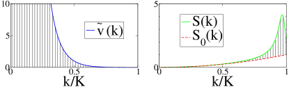
Figure 2: Shaded-area illustration of the two multiplicative contributions of the potential energy, defined in Eq. (3). Notice that even though the target structure factor $S_{0}(k)$ is monotonic in $k$, the actual structure factor $S(k)$ deviates from it and develops peaks, the first of which is shown here.

III Enumeration of the energy minima

We numerically study the classical ground states of the perfect-glass interactions and demonstrate their pattern uniqueness by showing that the enumeration entropy, defined by relation (1), is zero. We minimize the potential energy, using the low-storage Broyden–Fletcher–Goldfarb–Shanno algorithm Nocedal (1980); Liu and Nocedal (1989); Johnson , starting from random initial configurations, to find local minima of the potential energy surface. A random local minimum of the potential energy surface is deemed to be reached once the energy minimization routine finishes with a stringent tolerance of $\delta\Phi=10^{-11}$. Therefore, by repeating this process a sufficient number of times, we expect to find the global minimum of the potential energy surface. After $10^{7}$ to $10^{9}$ independent energy minimization trials, a lowest energy is achieved at least $10$ times, but often more than $10^{3}$ times (see Appendix A for details). Presumably, this is the ground state energy. Subsequently, we compare the ground-state configurations for pattern uniqueness. A particular ground-state configuration is taken to be a comparator, and then we compare it to every other ground-state configuration. Using an algorithm detailed in Appendix B, we attempt to find a translation, a rotation, and/or a reflection so that after these symmetry operations the comparator superposes onto the other ground state. After these symmetry operations are performed, if each particle in the comparator is within $10^{-5}L$ distance to a particle in the other ground state, then the two ground states are deemed to have the same pattern. Here $L$ denotes the side length of the simulation box. The ground state is considered pattern-unique if all of the ground-state configurations have the same pattern as the comparator.

We studied a total of 60 different combinations of parameters ($d$, $\alpha$, $\chi$, and $N$); see Appendix A for a complete list. These cases cover wide ranges of $N$ (between 10 and 70, including both prime $N$’s and composite $N$’s), $\alpha$ (between 0.5 and 6), and $\chi$ (between 1.7 and 2), in one, two, and three dimensions. For all cases, the ground state was found to be disordered and pattern-unique. The discovered ground states of the largest $N$ cases in the first three space dimensions are presented in Fig. 3.

Besides the ground states, we also study other minima of the potential energy surface. As Fig. 4 shows, as $N$ increases, the success rate (the probability that one finds the ground state through an energy minimization trial) decreases exponentially, and the number of discovered energy minima increases exponentially. This exponential rise of the number of higher minima is in agreement with what one has topographically for real glass formers Stillinger (2016). Compared to the $\alpha=1$ case, the $\alpha=6$ case possesses a higher success rate and fewer distinct energy levels. This is also expected because as we have discovered earlier, increasing $\alpha$ increases geometrical order in these glasses Zhang et al. (2016). Finally, Fig. 4 also shows that the ground state energy is roughly proportional to $N$ for both $\alpha$ values we presented.

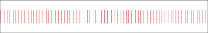
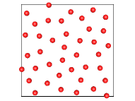
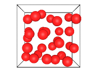
Figure 3: The disordered unique ground states of the perfect-glass potential for (top) $d=1$, $\alpha=6$, $\chi=1.75$, and $N=70$; (bottom left) $d=2$, $\alpha=6$, $\chi=1.87$, and $N=40$; and (bottom right) $d=3$, $\alpha=6$, $\chi=1.75$, and $N=30$. These figures illustrate a point presented in Ref. Zhang et al., 2016, namely, the particles experience a pair repulsion that is clearly observed when one calculates the pair correlation function.

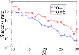
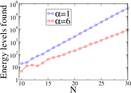
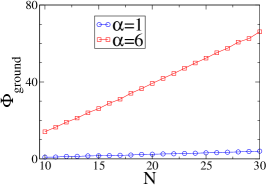
Figure 4: (left) The probability of finding the ground states by energy minimization for $d=1$, $\chi=2.00$, $\alpha=1$ and 6, and $10\leq N\leq 30$. (middle) The number of distinct energy local minima found by $10^{7}$ repeated energy minimizations for the same systems. (right) The ground-state energy of the same systems.

IV Calculation of the density of states

To further confirm ground-state uniqueness, we have also performed Wang-Landau Monte Carlo (WLMC) simulations on a perfect-glass system with $d=2$, $\alpha=1$, $\chi=1.89$, and $N=10$. The WLMC algorithm allows one to calculate the density of states $g(E)$ as a function of the potential energy Wang and Landau (2001) (or equivalently, the hyper-area of an iso-energy surface in the configuration space). Alternatively, for energy values very close to the ground state, one could also calculate $g(E)$ from the eigenvalues of the Hessian matrix by treating the system as an harmonic oscillator around the ground state. As detailed below, after considering the aforementioned trivial symmetry operations, we find very good agreement between the calculated $g(E)$’s from these two approaches, further verifying ground-state uniqueness.

IV.1 Density of states, $g(E)$, from the harmonic approximation

In this subsection, we calculate $g(E)$ using the harmonic approximation. For a $d$-dimensional configuration of $N$ particles, the configuration space is $dN$-dimensional. Of these $dN$ directions of the configuration space, $d$ directions correspond to translations of the whole configuration, which cause no energy change. The other $d(N-1)$ directions correspond to deformations, which generally change the potential energy. Near the classical ground state, such changes can be quantified by the eigenvalues of the Hessian matrix, $\lambda_{1}$, $\lambda_{2}$, $\cdots$, $\lambda_{d(N-1)}$. Let $E$ denote an energy that is slightly above the ground-state energy $E_{0}$; then the portion of the configuration space with potential energy $\Phi\leq E$ is given by the equation

$$E\geq E_{0}+\frac{\lambda_{1}}{2}x_{1}^{2}+\frac{\lambda_{2}}{2}x_{2}^{2}+\cdots+\frac{\lambda_{d(N-1)}}{2}x_{d(N-1)}^{2},$$ (4)

where $x_{1}$, $x_{2}$, $\cdots$, $x_{d(N-1)}$ are the deformations along each eigenvectors of the Hessian matrix. Equation (4) specifies a $d(N-1)$-dimensional ellipsoid, for which the hypervolume is

$$\mathcal{V}_{\mbox{vibrational}}=\frac{\pi^{d(N-1)/2}}{\Gamma[1+d(N-1)/2]}\prod_{j=1}^{d(N-1)}\sqrt{\frac{2\delta E}{\lambda_{j}}},$$ (5)

where $\frac{\pi^{d(N-1)/2}}{\Gamma[1+d(N-1)/2]}$ is the volume of a $d(N-1)$-dimensional hypersphere of unit radius and $\delta E=E-E_{0}$.

To obtain the total volume of the configuration space for which $\Phi\leq E$, one needs to multiply Eq. (5) with a few additional factors to account for trivial symmetry operations. First, there are $d$ independent translations, each contributing a factor of $\sqrt{N}L$, where $L$ is the side length of the simulation box. The factor $\sqrt{N}$ comes from the fact that translations correspond to diagonal movements in the configuration space. An additional factor, $f$, that depends on the space dimension and the simulation box shape, also needs to be included to account for rotations and reflections. For $d=2$ with square box, $f=8$, since such boxes allow rotations of $0^{\circ}$, $90^{\circ}$, $180^{\circ}$, and $270^{\circ}$, and a combination of any rotation with a chirality inversion. Lastly, particle permutations contribute a factor of $N!$. Overall, the total volume in the configuration space is

$$\mathcal{V}=N^{d/2}VfN!\frac{\pi^{d(N-1)/2}}{\Gamma[1+d(N-1)/2]}\prod_{j=1}^{d(N-1)}\sqrt{\frac{2\delta E}{\lambda_{j}}},$$ (6)

where $V=L^{d}$ is the volume of the simulation box.

The density of states is the surface area of the total volume in the configuration space for which $\Phi\leq E$, and is therefore the derivative of $\mathcal{V}$ to $E$:

$$\begin{split}g(E)=\frac{d\mathcal{V}}{dE}=N^{d/2}VfN!\frac{\pi^{d(N-1)/2}}{\Gamma[1+d(N-1)/2]}\\ \times\left(\prod_{j=1}^{d(N-1)}\sqrt{\frac{2}{\lambda_{j}}}\right)\frac{d(N-1)}{2}\delta E^{d(N-1)/2-1}.\end{split}$$ (7)

IV.2 Density of states, $g(E)$, from Wang-Landau Monte Carlo simulations

We now use the WLMC algorithm to calculate $g(E)$ for the perfect-glass system. To do so, we first divide the energy range $E_{0}\leq\Phi<10^{5}$ into $N_{\mbox{bin}}=2\times 10^{4}$ bins that are equidistant in a logarithmic scale. Let the minimum and maximum energies of a bin be $E_{\mbox{min}}$ and $E_{\mbox{max}}$, the WLMC algorithm allows one to calculate $\displaystyle g_{\mbox{bin}}=c\int_{E_{\mbox{min}}}^{E_{\mbox{max}}}g(E)dE$ over every bin, where $c$ is an unknown constant independent of the bin Wang and Landau (2001). We then determine $c$ by the condition $V^{N}=\displaystyle\int_{E_{0}}^{\infty}g(E)dE=\sum g_{\mbox{bin}}$, where the upper limit of the integration can be replaced with $10^{5}$, since $g(E)$ turns out to be negligible for very large $E$. We finally divide $\displaystyle g_{\mbox{bin}}$ with $(E_{\mbox{max}}-E_{\mbox{min}})$ to find out $g(E)$ at each bin.

We perform a total of $1500$ stages of Monte Carlo simulations, each consisting of $N_{\mbox{trial}}=4\times 10^{7}$ trial moves. In each trial move, a random particle is moved by a distance of $xyL$ in every direction, where $x$ is uniformly distributed between -1 and 1 and $y$ has a $50\%$ probability of being 0.2 and a $50\%$ probability of being 0.002. The WLMC algorithm has a tuning parameter, called the “modification factor” in Wang and Landau (2001), that affects its efficiency and accuracy. Following Ref. Belardinelli and Pereyra, 2007, we let this factor be $f=\exp\{\max[2N_{\mbox{bin}}/(N_{\mbox{trial}}i),\exp(-0.1i)]\}$ at the $i$th stage, where $\max(a,b)$ denotes the maximum value between $a$ and $b$.

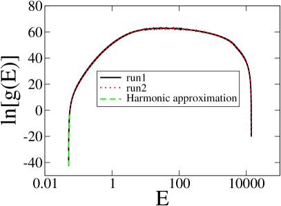
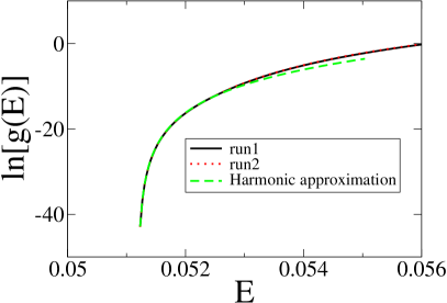
Figure 5: (Top) Natural logarithm of the density of states, $g(E)$, from two independent runs of WLMC simulations, and from the harmonic approximation. (Bottom) A zoomed-in view near the ground-state energy $E_{0}=0.0512129\ldots$.

We have performed two independent runs of the simulations detailed above. The resulting $g(E)$ is presented in Fig. 5 and compared with the $g(E)$ obtained from the harmonic approximation. At the lowest energies, $g(E)$ from both runs agree very well with that from the harmonic approximation, differing by less than $12\%$. If the ground state was two-fold degenerate, there would be a two-fold difference between the calculated $g(E)$. This verifies the uniqueness of the perfect-glass ground state.

From the density of states, we have also calculated the excess isochoric heat capacity $C_{V}$ of the system, which is given by

$$C_{V}=\frac{d\langle\Phi\rangle}{dk_{B}T},$$ (8)

where

$$\langle\Phi\rangle=\frac{\int Eg(E)\exp(-E/k_{B}T)dE}{\int g(E)\exp(-E/k_{B}T)dE}.$$ (9)

The heat capacity, presented in Fig. 6, starts at the harmonic value at $T=0$, and begins to rise because the shape of the potential energy landscape is such that the effective harmonic force constants are reduced in order to produce transition pathways to neighboring minima. The reduction of the local effective force constants increases the amount of configuration spaces associated with that particular level of the potential energy, and therefore increases the heat capacity. Eventually, $C_{V}$ levels off and decreases because the energy landscape becomes irrelevant at very high temperature.

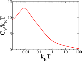
Figure 6: Isochoric heat capacity $C_{V}$ of the perfect-glass system of $d=2$, $\alpha=1$, $\chi=1.89$, and $N=10$. Here, the constant contribution to the heat capacity from the kinetic energy, $C_{V\mbox{, kinetic}}=dN/2$, is excluded.

V Conclusions and discussion

To summarize, all previously known disordered classical ground states are caused by interactions that allow continuous configurational deformations without energy change. These deformations also cause the ground state to possess large and extensive entropy. In contrast to these previous investigations, here we create disordered classical ground states by penalizing crystalline order, causing no ground-state degeneracy. These zero-entropy ground states are in sharp contrast with zero-entropy crystalline ground states, since the latter possess very high symmetry and long-range translational and rotational order.

Our discovery of unique disordered ground states impinge on the famous Kauzmann glass paradox Kauzmann (1948) and the associated “ideal glass” Debenedetti and Stillinger (2001). Historically, it was found that at some low but positive temperature, called the “Kauzmann temperature,” the extrapolated entropy of a supercooled liquid would be equal to and then apparently decline below that of the crystal, resulting in what has been called the “Kauzmann paradox.” This impossible scenario constitutes an entropy crisis. One resolution is to postulate that as the Kauzmann temperature is reached, the supercooled liquid must undergo a phase transition into an “ideal glass,” which is a glass with zero configurational entropy. This scenario is in contradistinction to the perfect-glass model, which does not require that the presence of a crystal and its thermodynamic properties has to provide a constraint on the behavior of the amorphous manifold of the configurations. Indeed, perfect-glass ground states can never be crystalline nor quasicrystalline. On the other hand, perfect-glass ground states and “ideal glasses” share one common feature: both states are disordered while having zero enumeration entropy.

We would like to stress that while the perfect-glasses interaction is not yet achievable in practice, it is an idealization that is nonetheless valuable because it teaches us what types of many-body molecular interactions are required to attain “unique” disorder and hence provides guidance to experimentalists to approximate such interactions in the laboratory with, for example, polymers Zhang et al. (2016).

Finally, we also expect our results to be useful in cryptography, where pseudo-random functions with tunable computational complexity are desired; for example, in deriving an encryption key from a password Krawczyk (2010). The task of finding a perfect-glass ground state suits this need, since its complexity can easily be tuned by changing a set of parameters ($d$, $N$, $\alpha$, and $\chi$).

Appendix A Summary of Results of the Numeration Studies

In Table LABEL:my-label, we summarize major results obtained from our enumeration studies for the different parameter combinations ($d$, $\alpha$, $\chi$, and $N$) that we used.

Table 1: List of all the parameter combinations ($d$, $\alpha$, $\chi$, and $N$) that we employed to carry out the enumeration studies and a summary of results for each combination, which includes the number of inherent structures that we generated, the number of times the ground state structure was achieved, the ground-state energy, the mean energy of inherent structures, and the number of distinct energy levels of inherent structures found.

$d$	$\alpha$	$\chi$	$N$	Number of inherent structures generated	Number of lowest-energy structures generated	Lowest energy	Mean energy (of inherent structures)	Number of distinct energies found
2	1	2.20	6	$10^{6}$	97510	0.0534	0.094867	37
2	0.5	1.89	10	$3\times 10^{7}$	1769	0.0059314	0.046363	34719
2	1	1.89	10	$3\times 10^{7}$	14442	0.0512129	0.126145	7398
2	2	1.89	10	$3\times 10^{7}$	1508436	0.835746	0.953847	339
2	6	1.89	10	$3\times 10^{7}$	5178002	2.73031	2.86945	34
2	1	1.87	16	$10^{8}$	147	0.0618558	0.178029	$2.16\times 10^{7}$
2	1	1.89	20	$10^{9}$	40	0.0664875	0.204629	$7.41\times 10^{8}$
2	6	1.89	20	$10^{8}$	265084	5.37199	5.74988	147590
2	6	1.90	30	$10^{8}$	1634	8.0647	8.57543	$4.08\times 10^{7}$
2	6	1.87	40	$10^{8}$	11	10.6843	11.3862	$9.10\times 10^{7}$
1	1	1.79	20	$2\times 10^{7}$	60490	0.517475	1.015135	3492
1	1	1.74	40	$5\times 10^{7}$	24	0.991197	1.849102	$3.06\times 10^{7}$
1	1	1.79	50	$10^{9}$	12	1.68337	2.94643	$8.45\times 10^{8}$
1	6	1.75	60	$10^{8}$	28	77.8601	79.7294	$5.46\times 10^{7}$
1	6	1.75	70	$10^{9}$	27	93.3095	95.7188	$5.94\times 10^{8}$
1	1	2.00	10	$10^{7}$	739724	0.866727	1.31398	20
1	1	2.00	11	$10^{7}$	651397	0.929444	1.42011	24
1	1	2.00	12	$10^{7}$	589273	1.2673	1.69868	48
1	1	2.00	13	$10^{7}$	242182	1.31007	1.87405	78
1	1	2.00	14	$10^{7}$	358037	1.53538	2.06303	109
1	1	2.00	15	$10^{7}$	142763	1.61837	2.29402	201
1	1	2.00	16	$10^{7}$	158544	1.69043	2.50381	351
1	1	2.00	17	$10^{7}$	105541	1.85802	2.74284	557
1	1	2.00	18	$10^{7}$	65853	1.98903	2.96204	959
1	1	2.00	19	$10^{7}$	27438	2.31345	3.17478	1578
1	1	2.00	20	$10^{7}$	22617	2.40054	3.4008	2613
1	1	2.00	21	$10^{7}$	15771	2.55858	3.64033	4527
1	1	2.00	22	$10^{7}$	20318	2.63018	3.85341	7645
1	1	2.00	23	$10^{7}$	9110	2.80526	4.06194	12665
1	1	2.00	24	$10^{7}$	5778	2.93012	4.289	21383
1	1	2.00	25	$10^{7}$	1754	3.1362	4.52102	36116
1	1	2.00	26	$10^{7}$	2095	3.21506	4.7385	60728
1	1	2.00	27	$10^{7}$	1261	3.45142	4.95513	100960
1	1	2.00	28	$10^{7}$	1618	3.60496	5.1805	168599
1	1	2.00	29	$10^{7}$	573	3.84163	5.39782	275767
1	1	2.00	30	$10^{7}$	518	4.01308	5.60469	442279
1	6	2.00	10	$10^{7}$	2715392	14.13106	14.2772	5
1	6	2.00	11	$10^{7}$	2749262	16.47931	16.8239	13
1	6	2.00	12	$10^{7}$	1432882	19.08413	19.325	15
1	6	2.00	13	$10^{7}$	470326	21.22258	21.5804	13
1	6	2.00	14	$10^{7}$	624508	23.95933	24.2088	22
1	6	2.00	15	$10^{7}$	578671	26.13922	26.7836	43
1	6	2.00	16	$10^{7}$	554290	28.93276	29.444	59
1	6	2.00	17	$10^{7}$	196175	31.03469	31.902	75
1	6	2.00	18	$10^{7}$	471502	34.10818	34.6142	102
1	6	2.00	19	$10^{7}$	224480	36.54381	37.2612	154
1	6	2.00	20	$10^{7}$	214371	39.26553	39.9763	204
1	6	2.00	21	$10^{7}$	73660	41.83513	42.6645	301
1	6	2.00	22	$10^{7}$	98901	44.40762	45.3614	422
1	6	2.00	23	$10^{7}$	69845	47.1069	48.1436	677
1	6	2.00	24	$10^{7}$	57822	49.86945	50.8796	887
1	6	2.00	25	$10^{7}$	57726	52.37915	53.5622	1343
1	6	2.00	26	$10^{7}$	26194	55.20688	56.4128	1966
1	6	2.00	27	$10^{7}$	22438	57.52615	59.1253	2853
1	6	2.00	28	$10^{7}$	12874	60.70169	61.9653	4022
1	6	2.00	29	$10^{7}$	2699	62.57372	64.6753	5898
1	6	2.00	30	$10^{7}$	10039	66.15001	67.5981	8796
3	1	1.70	10	$3\times 10^{7}$	1418	0.0020304	0.0196315	$1.04\times 10^{6}$
3	6	1.77	20	$3\times 10^{7}$	553282	1.05579	1.24064	945314
3	6	1.75	30	$3\times 10^{7}$	518	1.69167	1.88439	$2.51\times 10^{7}$

Appendix B Details of the Configuration Comparison Algorithm

Here provide details of the algorithm that we devised to compare two configurations to determine whether one of them can be superposed onto to the other after a translation, a rotation, and/or a reflection.

We begin with a description for the one-dimensional case for simplicity. For each configuration, we find a “characteristic vector” by the following steps:

• Find the closest pair of particles, $A$ and $B$. Find out their locations, $\mathbf{r}_{A}$ and $\mathbf{r}_{B}$.

• Find the distance from particle $A$ to its second closest neighbor particle, $d_{A}$; and the same distance for particle $B$, $d_{B}$.

• If $d_{A}>d_{B}$, then swap particles $A$ and $B$.

• The characteristic vector is $\mathbf{v}_{1}=\mathbf{r}_{B}-\mathbf{r}_{A}$.

The characteristic vector is invariant to configuration translations and particle permutations, and rotates or reflects if the configuration is rotated or reflected. Thus, if the two configurations are indeed related to each other through these trivial symmetry operations, then their characteristic vector must be related to each other by a constant 1 or -1, i.e.,

$$\mathbf{v}_{1}^{2}=R\mathbf{v}_{1}^{1},$$ (10)

where $\mathbf{v}_{1}^{j}$ is the characteristic vector of the $j$th configuration, and $R$ is either 1 or -1. If $R=1$, then the two configurations are not related to each other by any rotation or reflection. If $R=-1$, then the two configurations are related to each other by a $180^{\circ}$ rotation, or equivalently in one dimension, a reflection. The translation relating the two configurations can be found by the difference of the location of particle $A$: $\mathbf{t}=\mathbf{r}_{A}^{2}-R\mathbf{r}_{A}^{1}$, where the superscripts indicate different configurations. Having found the translation and rotation relating these configurations, one can verify that for each particle $j$ in the first configuration, at location $R\mathbf{r}_{j}^{1}+\mathbf{t}$ there is a particle in the second configuration. If so, and if the two configurations have the same number of particles, then these two configurations must be related to each other through symmetry operations.

To generalize this method to $d>1$ dimensions, one must find $d$ characteristic vectors, derived from $d$ closest particle pairs. Solving the following matrix equation gives the rotation and/or reflection matrix between the two configurations, $R$.

$$\begin{pmatrix}&&&\\ \mathbf{v}_{1}^{2}&\mathbf{v}_{2}^{2}&\cdots&\mathbf{v}_{d}^{2}\\ &&&\end{pmatrix}=R\begin{pmatrix}&&&\\ \mathbf{v}_{1}^{1}&\mathbf{v}_{2}^{1}&\cdots&\mathbf{v}_{d}^{1}\\ &&&\end{pmatrix}$$ (11)

where $\mathbf{v}_{i}^{j}$ is the $i$th characteristic vector of the $j$th configuration. The translation relating the two configurations can be found similarly by $\mathbf{t}=\mathbf{r}_{A}^{2}-R\mathbf{r}_{A}^{1}$, where $\mathbf{r}_{A}^{j}$ denotes the starting particle in finding the first characteristic vector in configuration $j$. Similar to the 1D case, the $j$th particle in configuration 1 still corresponds to a particle at $R\mathbf{r}_{j}^{1}+\mathbf{t}$ in configuration 2.

References

- Feynman (1955) R. P. Feynman, Prog. Low Temperature Phys. 1, 17 (1955).
- Kennedy et al. (1988) T. Kennedy, E. H. Lieb, and H. Tasaki, J. Stat. Phys. 53, 383 (1988).
- Sachdev (1992) S. Sachdev, Phys. Rev. B 45, 12377 (1992).
- Nakamura and Todo (2002) M. Nakamura and S. Todo, Phys. Rev. Lett. 89, 077204 (2002).
- Chen et al. (2016) C.-C. Chen, L. Muechler, R. Car, T. Neupert, and J. Maciejko, Phys. Rev. Lett. 117, 096405 (2016).
- Edwards and Anderson (1975) S. F. Edwards and P. W. Anderson, J. Phys. F 5, 965 (1975).
- Hansen and McDonald (1990) J.-P. Hansen and I. R. McDonald, Theory of simple liquids (Elsevier, 1990).
- Marinari et al. (1994a) E. Marinari, G. Parisi, and F. Ritort, J. Phys. A 27, 7615 (1994a).
- Marinari et al. (1994b) E. Marinari, G. Parisi, and F. Ritort, J. Phys. A 27, 7647 (1994b).
- Uche et al. (2006) O. U. Uche, S. Torquato, and F. H. Stillinger, Phys. Rev. E 74, 031104 (2006).
- Batten et al. (2008) R. D. Batten, F. H. Stillinger, and S. Torquato, J. Appl. Phys. 104, 033504 (2008).
- Zachary and Torquato (2011) C. E. Zachary and S. Torquato, Phys. Rev. E 83, 051133 (2011).
- Torquato et al. (2015) S. Torquato, G. Zhang, and F. H. Stillinger, Phys. Rev. X 5, 021020 (2015).
- Zhang et al. (2015) G. Zhang, F. H. Stillinger, and S. Torquato, Phys. Rev. E 92, 022119 (2015).
- Onsager (1949) L. Onsager, Ann. NY Acad. Sci. 51, 627 (1949).
- Alder and Wainwright (1957) B. J. Alder and T. E. Wainwright, J. Chem. Phys. 27, 1208 (1957).
- Frenkel (1999) D. Frenkel, Physica A 263, 26 (1999).
- Note (1) It should be stressed that this paper focuses on classical many-particle systems. If one includes spin systems (or equivalently, lattice-gas systems), which by definition lack continuous deformations, there are known examples of unique or pattern-unique classical ground states. In the “low-correlation” spin model Marinari et al. (1994a) and a subsequent simplified model Marinari et al. (1994b), the ground state is pattern-unique for a small fraction of system sizes but degenerate for other system sizes, while the degeneracy in the infinite-system-size limit is uncertain. (Although neither Ref. \rev@citealpmarinari1994replica nor Ref. \rev@citealpmarinari1994replica2 explicitly commented on the ground state degeneracy, we subsequently enumerated all possible spin configurations for 10-20 sites, and found that the ground states of the one-dimensional model described in Ref. \rev@citealpmarinari1994replica are degenerate, even after removing trivial translations and reflections, except for number of sites and . Ref. \rev@citealpmarinari1994replica2 stated that the models studied there has the same ground states as the model described in Ref. \rev@citealpmarinari1994replica.) Another example is the well-known spin-glass models, which has an unambiguously pattern-unique disordered ground state Edwards and Anderson (1975), but does so in a trivial way: the interaction is disordered (different for each pair of neighboring sites), causing the disordered ground state.
- Zhang et al. (2016) G. Zhang, F. H. Stillinger, and S. Torquato, Sci. Rep. 6 (2016).
- Torquato and Stillinger (2003) S. Torquato and F. H. Stillinger, Phys. Rev. E 68, 041113 (2003).
- Torquato (2016) S. Torquato, Phys. Rev. E 94, 022122 (2016).
- (22) Z. Ma and S. Torquato, J. Appl. Phys., 121, 244904 (2017).
- (23) A. Chremos and J. F. Douglas, Annalen der Physik, 1600342 (2017).
- (24) D. Hexner and D. Levine, Phys. Rev. Lett. 118, 020601 (2017).
- Kauzmann (1948) W. Kauzmann, Chem. Rev. 43, 219 (1948).
- Angell (1988) C. A. Angell, J. Phys. Chem. Solids 49, 863 (1988).
- Sastry (2001) S. Sastry, Nature 409, 164 (2001).
- Shintani and Tanaka (2006) H. Shintani and H. Tanaka, Nat. Phys. 2, 200 (2006).
- Ediger and Harrowell (2012) M. D. Ediger and P. Harrowell, J. Chem. Phys. 137, 080901 (2012).
- Gupta et al. (2015) S. Gupta, J. Stellbrink, E. Zaccarelli, C. N. Likos, M. Camargo, P. Holmqvist, J. Allgaier, L. Willner, and D. Richter, Phys. Rev. Lett. 115, 128302 (2015).
- Nocedal (1980) J. Nocedal, Math. Comp. 35, 773 (1980).
- Liu and Nocedal (1989) D. C. Liu and J. Nocedal, Math. Programming 45, 503 (1989).
- (33) S. G. Johnson, “The nlopt nonlinear-optimization package,” Http://ab-initio.mit.edu/nlopt.
- Stillinger (2016) F. H. Stillinger, Energy Landscapes, Inherent Structures, and Condensed-Matter Phenomena (Princeton University Press, 2016).
- Wang and Landau (2001) F. Wang and D. P. Landau, Phys. Rev. Lett. 86, 2050 (2001).
- Belardinelli and Pereyra (2007) R. E. Belardinelli and V. D. Pereyra, J. Chem. Phys. 127, 184105 (2007).
- Debenedetti and Stillinger (2001) P. G. Debenedetti and F. H. Stillinger, Nature 410, 259 (2001).
- Krawczyk (2010) H. Krawczyk, in Advances in Cryptology-Crypto 2010 (Springer, 2010) pp. 631–648.