Sliced-Inverse-Regression-Aided Rotated Compressive Sensing Method for Uncertainty Quantification

Abstract

Compressive-sensing-based uncertainty quantification methods have become a powerful tool for problems with limited data. In this work, we use the sliced inverse regression (SIR) method to provide an initial guess for the alternating direction method, which is used to enhance sparsity of the Hermite polynomial expansion of stochastic quantity of interest. The sparsity improvement increases both the efficiency and accuracy of the compressive-sensing-based uncertainty quantification method. We demonstrate that the initial guess from SIR is suitable for cases when the available data are limited (Algorithm 4). We also propose another algorithm (Algorithm 5) that performs dimension reduction first with SIR. Then it constructs a Hermite polynomial expansion of the reduced model. This method affords the ability to approximate the statistics accurately with even less available data. Both methods are non-intrusive and require no a priori information of the sparsity of the system. The effectiveness of these two methods (Algorithms 4 and 5) are demonstrated using problems with up to $500$ random dimensions.

Keywords compressive sensing, uncertainty quantification, sliced inverse regression,iterative rotation, alternating direction method.

1 Introduction

Surrogate model is a powerful tool in studying uncertainty quantification (UQ). For example, spectral-method-based surrogate models, including the polynomial chaos expansion (PCE) [19] and generalized polynomial chaos (gPC) [51] methods, are widely used for UQ in engineering and computational sciences. In the gPC and PCE methods, a quantity of interest (QoI) $u$ (e.g, velocity, temperature, etc.) depends on $d$-dimensional ($d<\infty$) random variables $\bm{\xi}=(\xi_{1},\xi_{2},\cdots,\xi_{d})^{\mathsf{T}}$, which are used to represent stochastic initial and boundary conditions or other unknown properties, can be approximated as

$$u(\bm{\xi})=\sum_{n=1}^{N}c_{n}\psi_{n}(\bm{\xi})+\varepsilon(\bm{\xi}),$$ (1)

where $\varepsilon$ is the truncation error; $N$ is a positive integer; $c_{n}$ are coefficients; and $\psi_{n}$ are multivariate orthonormal polynomials satisfying

$$\mathbb{E}\left\{{\psi_{i}(\bm{\xi})\psi_{j}(\bm{\xi})}\right\}=\int_{\mathbb{R}^{d}}\psi_{i}(\bm{x})\psi_{j}(\bm{x})\rho_{{}_{\bm{\xi}}}(\bm{x})\mathrm{d}\bm{x}=\delta_{i,j},$$ (2)

where $\rho_{{}_{\bm{\xi}}}(\bm{x})$ is the probability density function (PDF) of $\bm{\xi}$ and $\delta_{ij}$ is the Kronecker delta function. Here $\bm{\xi}$ is defined on the probability space $(\Omega,\mathcal{F},P)$, where $\Omega$ is the abstract set of elementary events, $\mathcal{F}$ is a $\sigma$-algebra of subsets of $\Omega$ and $P$ is the probability measure on $\mathcal{F}$. The QoI $u$ is defined on the Hilbert space $\mathcal{H}=L^{2}(\Omega,\mathcal{F},P)$ that consists of real-valued random variables defined on $(\Omega,\mathcal{F},P)$ with finite second moment and is equipped with a inner product $(u,v)_{L^{2}}=\int_{\Omega}uv\mathrm{d}P$, for $u,v\in\mathcal{H}$. For example, when $\{\xi_{i}\}_{i=1}^{d}$ are independent and identically distributed (i.i.d.) Gaussian random variables, i.e., $\bm{\xi}\sim\mathcal{N}(\bm{0},\mathbf{I})$, $P$ is the Gaussian measure, and $\psi_{n}$ are normalized multi-variate Hermite polynomials. For this case, systematic studies of convergence of PCE and gPC [7, 17] indicate that $\sum_{n=1}^{N}c_{n}\psi_{n}(\bm{\xi})$ converges to $u(\bm{\xi})$ in $L^{2}$ as $N\rightarrow\infty$. For the convergence of more general cases, we refer the interested readers to [17].

Both intrusive and non-intrusive methods [19, 51, 43, 50, 18, 5] are extensively used to compute the gPC coefficients $\bm{c}=(c_{1},c_{2},\cdots,c_{N})^{\mathsf{T}}$. Non-intrusive methods are more useful when the model used to obtain $u$ is especially complex. These methods utilize training sets $\{(\bm{\xi}^{q},u^{q})\}_{q=1}^{M}$ to approximate coefficients $\bm{c}$. Here, $\bm{\xi}^{q}$ are samples of input based on $\rho_{{}_{\bm{\xi}}}$, and $u^{q}$ are corresponding samples of the output $u^{q}=u(\bm{\xi}^{q})$ obtained from the computational model. In many applications, it can be very costly to obtain $u^{q}$. Because of this, it often is $M<N$ or even $M\ll N$, making the following linear system underdetermined:

$$\mathbf{\Psi}\bm{c}=\bm{u}-\bm{\varepsilon},$$ (3)

where $\bm{u}=(u^{1},u^{2},\cdots,u^{M})^{\mathsf{T}}$ is the vector of output samples, $\mathbf{\Psi}$ is an $M\times N$ matrix with $\Psi_{ij}=\psi_{j}(\bm{\xi}^{i})$ (where $j=1,\cdots,N$ and $i=1,\cdots,M$), and $\bm{\varepsilon}=(\varepsilon^{1},\varepsilon^{2},\cdots,\varepsilon^{M})^{\mathsf{T}}$ is a vector of error samples with $\varepsilon^{q}=\varepsilon(\bm{\xi}^{q})$ (where $q=1,\cdots,M$). The compressive sensing method has been shown to be effective at solving the underdetermined Eq. (3) when $\bm{c}$ is sparse [9, 15, 8, 6], i.e., solving

$$(P_{1,\epsilon}):\qquad\operatorname*{arg\,min}_{\hat{\bm{c}}}\|\hat{\bm{c}}\|_{1},\text{~{}~{}subject to~{}~{}}\|\mathbf{\Psi}\hat{\bm{c}}-\bm{u}\|_{2}\leq\epsilon,$$

to approximate $\bm{c}$ in Eq. (3) with $\hat{\bm{c}}$ (see Section 2.2). It has been used to solve UQ problems in various settings [16, 52, 55, 27, 34, 20, 23, 40, 35].

Several approaches have been developed to enhance the efficiency of solving Eq. (3) in UQ applications, including weighted/re-weighted $\ell_{1}$ minimization, which assigns a weight to each $c_{n}$ and solves a weighted $\ell_{1}$ minimization problem to enhance the sparsity [11, 55, 34, 37]; smart sampling strategies to better the property of $\mathbf{\Psi}$ [36, 20]; and adaptive basis selection to reduce the number of unknowns [23].

In [27, 56, 58], an approach to enhance the sparsity of $\bm{c}$ through the rotation of the random vector $\bm{\xi}$ has been proposed. This method aims to find a rotation $g:\mathbb{R}^{d}\mapsto\mathbb{R}^{d}$ that maps $\bm{\xi}$ to a new set of random variables $\bm{\eta}=(\eta_{1},\eta_{2},\cdots,\eta_{d})^{\mathsf{T}}$ as $\bm{\eta}=g(\bm{\xi})=\mathbf{A}\bm{\xi}$ (where $\mathbf{A}\mathbf{A}^{\mathsf{T}}=\mathbf{I}$) such that the gPC expansion of $u$ with respect to $\bm{\eta}$ is sparser. Specifically,

$$u(\bm{\xi})\approx\sum_{n=1}^{N}c_{n}\psi_{n}(\bm{\xi})=\sum_{n=1}^{N}\tilde{c}_{n}\psi_{n}(\bm{\eta}(\bm{\xi}))\approx u(\bm{\eta}(\bm{\xi})),$$ (4)

and $\tilde{\bm{c}}=(\tilde{c}_{1},\tilde{c}_{2},\cdots,\tilde{c}_{N})^{\mathsf{T}}$ is sparser than $\bm{c}$. Hence, $\tilde{\bm{c}}$ can be approximated more accurately using the compressive sensing method. Subsequently, the enhancement of the sparsity enables the compressive sensing algorithm to obtain a more accurate approximation of $u$ in the $L^{2}$ sense. In other words, $(P_{1,\epsilon})$ is modified as (see Section 3.1)

$$(P_{1,\varepsilon}^{R}):\qquad\operatorname*{arg\,min}_{\hat{\bm{c}},~{}\mathbf{A}}\|\hat{\bm{c}}\|_{1},\quad\text{subject to}\quad\|\mathbf{\Psi}(\mathbf{A})\hat{\bm{c}}-\bm{u}\|_{2}\leq\epsilon,\mathbf{A}^{\mathsf{T}}\mathbf{A}=\mathbf{I},$$

where $\mathbf{\Psi}(\mathbf{A})$ is an $M\times N$ matrix and $(\mathbf{\Psi}(\mathbf{A}))_{ij}=\psi_{j}(\mathbf{A}\bm{\xi}^{i})$. An alternating direction method (ADM) has been developed to iteratively identify $\tilde{\bm{c}}$ and the rotation matrix $\mathbf{A}$ based on the gradients of $u$. Of note, this ADM method does not guarantee to identify the exact solution of $(P_{1,\epsilon}^{R})$. It helps to identify an approximation of $\mathbf{A}$ such that a sparser representation of $u$ can be obtained.

In the present work, we improve the efficiency of the ADM method by using the sliced inverse regression (SIR) method to provide the initial guess of the rotation matrix $\mathbf{A}$ (Algorithm  4). The SIR method is used in statistics to identify important low-dimensional subspaces based on the training set $\{(\bm{\xi}^{q},u^{q})\}_{q=1}^{M}$. We demonstrate that the initial guess from SIR helps to improve the ADM algorithm accuracy in some cases. Moreover, we propose another method that uses SIR to reduce the number of dimensions from $d$ to $\tilde{d}$, then employs ADM method to construct a “reduced” gPC expansion of $u$ (Algorithm 5). In this case, the dimension reduction performed by SIR reduces the number of unknowns $N$, which can be prohibitively large for the compressive sensing method when $d$ is large. To sum up, both new algorithms start with SIR to identify low-dimensional subspaces. Then, this information is used in the ADM algorithm with (Algorithm 4) or without (Algorithm 5) dimension reduction to improve the accuracy of compressive-sensing-based surrogate model construction for UQ problems. In this paper, we focus on problems where uncertainty (uncertain parameters) can be described by $d$-dimensional i.i.d. Gaussian random variables $\bm{\xi}\sim\mathcal{N}(\bm{0},\mathbf{I})$. This assumption is used broadly in physical and engineering problems, and it naturally fits the SIR method’s requirement (see Section 2.4).

The paper includes a brief review of UQ, compressive sensing methods, and the SIR method in Section 2. Section 3 describes the proposed schemes, Algorithm 4 and Algorithm 5. Numerical results are presented in Section 4, and the conclusions follow in Section 5.

2 Review of compressive-sensing-based gPC and SIR methods

This section includes a brief review of the compressive-sensing-based gPC and SIR methods, which form the basis of the new method proposed in Section 3.

2.1 Hermite polynomial expansions

When QoI of the problem relies on i.i.d Gaussian random variables, it can be represented with a gPC expansion with basis functions constructed by tensor products of univariate Hermite polynomials. Given a multi-index $\bm{\alpha}=(\alpha_{1},\alpha_{2},\cdots,\alpha_{d}),\alpha_{i}\in\mathbb{N}\cup\{0\}$, we set

$$\psi_{\bm{\alpha}}(\bm{\xi})=\psi_{\alpha_{1}}(\xi_{1})\psi_{\alpha_{2}}(\xi_{2})\cdots\psi_{\alpha_{d}}(\xi_{d}).$$ (5)

A gPC expansion up to $P$-th order implies that $|\bm{\alpha}|\leq P$ for all $\psi_{\bm{\alpha}}$ used in the expansion. For two different multi-indices $\bm{\alpha}_{i}=((\bm{\alpha}_{i})_{{}_{1}},(\bm{\alpha}_{i})_{{}_{2}},\cdots,(\bm{\alpha}_{i})_{{}_{d}})$ and $\bm{\alpha}_{j}=((\bm{\alpha}_{j})_{{}_{1}},(\bm{\alpha}_{j})_{{}_{2}},\cdots,(\bm{\alpha}_{j})_{{}_{d}})$, the Hermite polynomials satisfy the following orthogonality condition:

$$\int_{\mathbb{R}^{d}}\psi_{\bm{\alpha}_{i}}(\bm{x})\psi_{\bm{\alpha}_{j}}(\bm{x})\rho_{{}_{\bm{\xi}}}(\bm{x})\mathrm{d}\bm{x}=\delta_{\bm{\alpha}_{i}\bm{\alpha}_{j}}=\delta_{(\bm{\alpha}_{i})_{{}_{1}},(\bm{\alpha}_{j})_{{}_{1}}}\delta_{(\bm{\alpha}_{i})_{{}_{2}},(\bm{\alpha}_{j})_{{}_{2}}}\cdots\delta_{(\bm{\alpha}_{i})_{{}_{d}},(\bm{\alpha}_{j})_{{}_{d}}},$$ (6)

where $\delta_{(\alpha_{i})_{{}_{2}},(\alpha_{j})_{{}_{2}}}$ are Kronecker delta functions,

$$\rho_{{}_{\bm{\xi}}}(\bm{x})=\rho_{{}_{\xi_{1}}}(x_{1})\rho_{{}_{\xi_{2}}}(x_{2})\cdots\rho_{{}_{\xi_{d}}}(x_{d})$$ (7)

and $\rho_{{}_{\xi_{i}}}(x_{i})=\frac{1}{\sqrt{2\pi}}\mathrm{e}^{-x_{i}^{2}/2}$ because $\xi_{i}$ are independent Gaussian random variables. In general, when $\xi_{i}$ satisfy other distribution, $\psi_{\bm{\alpha}}$ can be represented as a tensor product of univariate polynomials associated with the PDF of $\xi_{i}$. In the following, for simplicity we denote $\psi_{\bm{\alpha}_{i}}(\bm{\xi})$ as $\psi_{i}(\bm{\xi})$, and the gPC expansion used is in the form of Eq. (1).

2.2 Compressive sensing

We first introduce the notation that denotes number of non-zeros entries in a vector $\bm{x}=(x_{1},x_{2},\cdots,x_{N})$ [14, 9, 6]:

$$\|\bm{x}\|_{0}\stackrel{{\scriptstyle\textrm{def}}}{{=}}\#\{i:x_{i}\neq 0\}.$$ (8)

The vector $\bm{x}$ is called $s$-sparse if $\|\bm{x}\|_{0}\leq s$, and $\bm{x}$ is considered a sparse vector if $s\ll N$. In practice, a very few systems have a truly sparse gPC coefficients $\bm{c}$. However, in many cases, the $\bm{c}$ is “compressible”, i.e., only a few entries make significant contribution to its $\ell_{1}$ norm. Here, the $\ell_{1}$ norm is defined as $\|\bm{x}\|_{1}\stackrel{{\scriptstyle\textrm{def}}}{{=}}\sum_{n=1}^{N}|x_{n}|.$ Subsequently, $\bm{x}$ is considered sparse if $\|\bm{x}-\bm{x}_{s}\|_{1}$ is small for $s\ll N$, and this definition of sparsity is widely used in error estimation. The vector $\bm{x}_{s}$ is equal to $\bm{x}$ with all but the $s$-largest entries set to zero [8].

The sparse vector $\bm{c}$ in Eq. (3) can be approximated by solving the following $\ell_{1}$ minimization problem:

$$(P_{1,\epsilon}):\qquad\operatorname*{arg\,min}_{\hat{\bm{c}}}\|\hat{\bm{c}}\|_{1},\text{~{}~{}subject to~{}~{}}\|\mathbf{\Psi}\hat{\bm{c}}-\bm{u}\|_{2}\leq\epsilon,$$ (9)

where $\epsilon=\|\bm{\varepsilon}\|_{2}$. To obtain the error bound in $(P_{1,\epsilon})$, the restricted isometry property (RIP) constant is introduced [10]. For each integer $s=1,2,\cdots$, the restricted isometry constant $\delta_{s}$ of a matrix $\mathbf{\Psi}$ is defined as the smallest number such that

$$(1-\delta_{s})\|\bm{x}\|_{2}^{2}\leq\|\mathbf{\Psi}\bm{x}\|_{2}^{2}\leq(1+\delta_{s})\|\bm{x}\|_{2}^{2}$$ (10)

holds for all $s$-sparse vectors $\bm{x}$. Candès et al. [10] showed that if the matrix $\mathbf{\Psi}$ satisfies $\delta_{2s}<\sqrt{2}-1$ (i.e., $\mathbf{\Psi}$ satisfies “RIP”), and $\|\bm{\varepsilon}\|_{2}\leq\epsilon$, then solution $\hat{\bm{c}}$ to $(P_{1,\epsilon})$ obeys

$$\|\bm{c}-\hat{\bm{c}}\|_{2}\leq C_{1}\epsilon+C_{2}\dfrac{\|\bm{c}-\bm{c}_{s}\|_{1}}{\sqrt{s}},$$ (11)

where $C_{1}$ and $C_{2}$ are constants, and $\bm{c}$ is the exact vector we aim to approximate. This result implies that the upper bound of the error relates to the truncation error and the sparsity of $\bm{c}$, which is reflected in the first and second terms on the right-hand side of Eq. (11), respectively.

In practice, the re-weighted $\ell_{1}$ minimization approach [11] is an improvement of the $\ell_{1}$ minimization method, which enhances the accuracy of estimating $\bm{c}$. It modifies $(P_{1,\epsilon})$ as

$$(P_{1,\epsilon}^{W}):\qquad\operatorname*{arg\,min}_{\hat{\bm{c}}}\|\mathbf{W}\hat{\bm{c}}\|_{1},~{}\text{subject to}~{}\|\mathbf{\Psi}\hat{\bm{c}}-\bm{u}\|_{2}\leq\epsilon,$$ (12)

where $\mathbf{W}$ is a diagonal matrix: $\mathbf{W}=\text{diag}(w_{1},w_{2},\cdots,w_{N})$. $(P_{1,\epsilon})$ can be considered as a special case of $(P_{1,\epsilon}^{W})$ with $\mathbf{W}=\mathbf{I}$. The elements $w_{i}$ of the diagonal matrix can be estimated iteratively [11, 55]: in the $l$-th iteration, $w_{i}$ is set to $w_{i}^{(l)}=1/(|\hat{c}_{i}^{(l-1)}|+\delta)$, where $\hat{c}_{i}^{(l-1)}$ is the solution from the last iteration and $\hat{c}_{i}^{(0)}$ is the solution of the standard $\ell_{1}$ minimization problem $(P_{1,\epsilon})$. The parameter $\delta>0$ is introduced to provide stability and to ensure that a zero-valued component in $\hat{\bm{c}}^{(l)}$ does not prohibit a non-zero estimate at the next step, i.e., it ensures that the weights do not become infinity. Candés et al. [11] suggest performing two or three iterations of this procedure. The error bound of the re-weighted $\ell_{1}$ minimization (see [33]) takes the same form as Eq. (11) with different constants $C_{1}$ and $C_{2}$. Moreover, the error term $\epsilon$ in $(P_{1,\epsilon})$ is usually not known a priori, and, in the present work, we use cross-validation to estimate it (see the Appendix for the details).

2.3 Compressive-sensing-based gPC methods

Given $M$ samples of $\bm{\xi}$, we use gPC expansion Eq. (1) to represent the uncertainty of QoI $u$, and we have

$$u(\bm{\xi}^{q})=\sum_{n=1}^{N}c_{n}\psi(\bm{\xi}^{q})+\varepsilon(\bm{\xi}^{q}),\quad q=1,2,\cdots,M,$$ (13)

which can be rewritten as Eq. (3). A typical approach to compressive-sensing based-gPC is summarized in Algorithm 1 [56].

Algorithm 1 Compressive-sensing-based gPC method.

1:  Generate input samples $\bm{\xi}^{q},q=1,2,\cdots,M$ based on the distribution of $\bm{\xi}$.

2:  Generate output samples $u^{q}=u(\bm{\xi}^{q})$ by solving the complete model, e.g., running simulations, solvers, etc.

3:  Select gPC basis functions $\{\psi_{n}\}_{n=1}^{N}$ associated with $\bm{\xi}$ and then generate the measurement matrix $\mathbf{\Psi}$ by setting $\Psi_{ij}=\psi_{j}(\bm{\xi}^{i})$.

4:  Solve the optimization problem $(P_{1,\epsilon})$:

$$\operatorname*{arg\,min}_{\hat{\bm{c}}}\|\hat{\bm{c}}\|_{1},~{}\text{subject to}\|\mathbf{\Psi}\hat{\bm{c}}-\bm{u}\|_{2}\leq\epsilon,$$

where $\bm{u}=(u^{1},u^{2},\cdots,u^{M})^{\mathsf{T}}$, and $\epsilon$ is obtained by cross-validation (see Algorithm 6 in Appendix). If the re-weighted $\ell_{1}$ method is employed, solve $(P_{1,\epsilon}^{W})$ instead.

5:  Construct the gPC expansion as $u(\bm{\xi})\approx\sum_{n=1}^{N}\hat{c}_{n}\psi_{n}(\bm{\xi})$.

2.4 Sliced Inverse Regression

SIR is an effective approach for seeking the important subspaces in the parameter space [28]. As an illustration, consider $u(\bm{\xi})=u(\xi_{1},\xi_{2})=(\xi_{1}+\xi_{2})^{2}$. Then, if we define $\hat{\mathbf{A}}=(1/\sqrt{2},1/\sqrt{2})$ and $\eta_{1}=\hat{\mathbf{A}}\bm{\xi}$, $u$ only depends on $\eta_{1}$. Consequently, the dimension is reduced from $d=2$ to reduced dimension $\tilde{d}=1$ because we only need one input random variable to fully capture the statistical property of $u$. Unlike the outer product gradients (OPGs) [22, 48] or active subspace method [12] where gradients information is used to identify $\hat{\mathbf{A}}$, the SIR method uses conditional expectation $\mathbb{E}\left\{{\bm{\xi}|u}\right\}$. $\mathbb{E}\left\{{\bm{\xi}|u}\right\}$ is a $d$-dimensional random vector because $u$ is random. As $u$ varies, $\mathbb{E}\left\{{\bm{\xi}|u}\right\}$ draws a curve in the parameter space, which is called inverse regression curve. It has been shown that this curve resides in the desired subspace for dimension reduction (named central subspace) if $\bm{\xi}$ follows an elliptically symmetric distribution [28], e.g., the multivariate Gaussian distribution. Based on this property, we choose the matrix $\hat{\mathbf{A}}$ such that its columns consist of the eigenvectors corresponding to the non-zero eigenvalues of the covariance matrix $\mathbf{V}=\text{var}\left\{\mathbb{E}\left\{{\bm{\xi}|u}\right\}\right\}$. An estimate of $\hat{\mathbf{A}}$ is summarized in Algorithm 2, originally proposed in [28]. A software package implementing the algorithm is available in [47].

Algorithm 2 Sliced inverse regression algorithm.

1:  Generate i.i.d. samples of input parameters $\bm{\xi}^{i}$, $i=1,...,M$, and compute the corresponding values of QoI $u^{i}$.

2:  Divide the range of $u^{i}$, i.e., $[\min(u^{i}),\max(u^{i})]$, into $H$ non-overlapping slices, $J_{1},...,J_{H}$: $[u_{0},u_{1}),[u_{1},u_{2}),\cdots,[u_{H-1},u_{H}]$, where $\min(u^{i})=u_{0}<u_{1}<u_{2}<\cdots<u_{H-1}<u_{H}=\max(u^{i})$, each containing approximately an equal number of data points.

3:  Compute the within-slice mean of $\bm{\xi}$ over each slice, which is a crude estimate of the conditional expectation $\mathbb{E}\left\{{\bm{\xi}|u}\right\}$:

$$\bar{\bm{\xi}}_{h}=\frac{1}{n_{h}}\sum_{u^{i}\in J_{h}}\bm{\xi}^{i},\;h=1,...,H,$$

where $n_{h}$ is the number of data points falling in the $h$th slice.

4:  Compute the $d\times d$ matrix

$$\mathbf{V}=\sum_{i=1}^{H}\frac{n_{h}}{n}\bar{\bm{\xi}}_{h}\bar{\bm{\xi}}_{h}^{\mathsf{T}}.$$

This is the sample estimate of the covariance matrix of the random vector $E(\bm{\xi}|\tilde{u})$, where $\tilde{u}=\sum_{h=1}^{H}hI(u\in J_{h})$ and $I(\cdot)$ is the indicator function.

5:  Compute the eigen-decomposition of $\mathbf{V}$: $\mathbf{V}=\mathbf{U}_{V}\mathbf{\Lambda}_{V}\mathbf{U}_{V}^{\mathsf{T}}$, where $\mathbf{\Lambda}_{V}$ is a diagonal matrix consists of eigenvalues: $(\mathbf{\Lambda}_{V})_{ii}=(\lambda_{V})_{i}$ ($1\leq i\leq d$) with $(\lambda_{V})_{1}\geq(\lambda_{V})_{2}\geq\cdots\geq(\lambda_{V})_{d}\geq 0$ and $\mathbf{U}_{V}\mathbf{U}_{V}^{\mathsf{T}}=\mathbf{I}$.

6:  Report the estimated transformation matrix as a submatrix consisting of the first $\tilde{d}$ (reduced dimension) rows of $\mathbf{U}_{V}^{\mathsf{T}}$: $\hat{\mathbf{A}}=[(\mathbf{U}_{V})_{1},...,(\mathbf{U}_{V})_{\tilde{d}}]^{\mathsf{T}}$, where $\tilde{d}\leq d$.

Of note, most applications of SIR are concerned with dimension reduction by choosing $\tilde{d}$ to be as small as possible, i.e., smaller than $d$ (see Algorithm 2). In this work, we use this setting in Algorithm 5. On the other hand, we use $\hat{\mathbf{A}}$ with $\tilde{d}=d$ to obtain an initial guess for the ADM algorithm (see Algorithm 4).

Notably, SIR can be considered as an approach within the framework of sufficient dimension reduction (SDR). To simplify the model $u(\bm{\xi})$, an effective modeling strategy is to assume that only a few subspaces make major contributions to $u$. A formal definition tailored from [28] in [30] is as follows:

Definition: Given the $d$-dimensional model $u(\bm{\xi})$, a dimension reduction is a mapping from the $d$-dimensional input to a $\tilde{d}$-dimensional vector, $\bm{\eta}=\mathbf{A}\bm{\xi}$, where $\mathbf{A}\in\mathbb{R}^{\tilde{d}\times d}$, $\tilde{d}<d$, $\mathbf{A}\mathbf{A}^{\mathsf{T}}=\mathbf{I}$ is the identity matrix. A dimension reduction is sufficient if the following equation holds for any $\bm{\xi}\in\mathbb{R}^{d}$:

$$u(\bm{\xi})=u(\mathbf{A}^{\mathsf{T}}\mathbf{A}\bm{\xi})\equiv f(\mathbf{A}^{\mathsf{T}}\bm{\eta}).$$

In other words, $u$ only relies on $\tilde{d}$ variables $\eta_{1},\eta_{2},\cdots,\eta_{\tilde{d}}$. For example, the active subspace method [12], basis adaptation method [44], and SIR method aim to identify this low-dimensional structure by computing $\mathbf{A}$ in a different manner.

3 SIR-aided Rotated Compressive Sensing Method

This section details two new applications of the SIR method for the compressive-sensing-based gPC, which is the main contribution of this work.

3.1 Alternating direction method for increasing sparsity

In practical problems, if the truncation error $\epsilon$ is sufficiently small, then the second term on the right-hand side of Eq. (11) dominates the upper bound of the error. Hence, to improve the accuracy of the gPC expansion, we need to decrease $\|\bm{c}-\bm{c}_{s}\|_{1}/\sqrt{s}$. Our goal is to seek $\mathbf{A}$ (and $\bm{\eta}=\mathbf{A}\bm{\xi}$) such that in Eq. (4), $\|\tilde{\bm{c}}-\tilde{\bm{c}}_{s}\|_{1}<\|\bm{c}-\bm{c}_{s}\|_{1}$. In other words, we rewrite the standard $\ell_{1}$ minimization problem $(P_{1,\epsilon})$ as

$$(P_{1,\varepsilon}^{R}):\qquad\operatorname*{arg\,min}_{\hat{\bm{c}},~{}\mathbf{A}}\|\hat{\bm{c}}\|_{1},\quad\text{subject to}\quad\|\mathbf{\Psi}(\mathbf{A})\hat{\bm{c}}-\bm{u}\|_{2}\leq\epsilon,\mathbf{A}^{\mathsf{T}}\mathbf{A}=\mathbf{I}.$$ (14)

where $\mathbf{\Psi}(\mathbf{A})$ is a matrix and $(\mathbf{\Psi}(\mathbf{A}))_{ij}=\psi_{j}(\mathbf{A}\bm{\xi}^{i})$. In the ADM algorithm proposed in [56], gradient information is used to identify $\mathbf{A}$. A “gradient matrix” is defined as

$$\mathbf{G}\stackrel{{\scriptstyle\textrm{def}}}{{=}}\mathbb{E}\left\{{\nabla u(\bm{\xi})\otimes\nabla u(\bm{\xi})}\right\}=\mathbf{U}\mathbf{\Lambda}\mathbf{U}^{\mathsf{T}},\quad\mathbf{U}\mathbf{U}^{\mathsf{T}}=\mathbf{I},$$ (15)

where $\mathbf{G}$ is symmetric, $\nabla u(\bm{\xi})=(\partial u/\partial\xi_{1},\cdots,\partial u/\partial\xi_{d})^{\mathsf{T}}$ is a column vector, $\mathbf{U}=(\bm{U}_{1},\cdots,\bm{U}_{d})$ is an orthogonal matrix consisting of eigenvectors $\bm{U}_{i}$, and $\mathbf{\Lambda}=\text{diag}(\lambda_{1},\cdots,\lambda_{d})$ with $\lambda_{1}\geq\lambda_{2}\geq\cdots\lambda_{d}\geq 0$ is a diagonal matrix with elements representing variation of the system along the respective eigenvectors. Then, $\mathbf{A}$ can be chosen as the unitary matrix $\mathbf{U}^{\mathsf{T}}$, which defines a rotation in $\mathbb{R}^{d}$ projecting $\bm{\xi}$ on the eigenvectors $\bm{U}_{i}$. If only a few $\lambda_{i}$s are very large (compared with other $\lambda_{i}$s), the rotation that maps $\bm{\xi}$ to $\bm{\eta}=\mathbf{A}\bm{\xi}$ helps to concentrate the dependence of $u$ primarily on those few new random variables $\eta_{i}$ due to the larger variation of $u$ along the directions of the corresponding eigenvectors. Therefore, the resulting coefficients $\tilde{\bm{c}}$ can be sparser than $\bm{c}$. This approach of constructing $\mathbf{G}$ from active subspace (proposed in [12]) is similar to the method of OPGs in statistics [22, 48]. The gradient of $u$ also has been used to improve the efficiency of compressive sensing in the gradient-enhanced method [31, 23, 35].

Because the explicit form of $u$ or $\nabla u$ is unknown, an ADM algorithm is proposed to identify $\mathbf{A}$ and $\tilde{c}$ iteratively. As noted in the introduction, this work aims to solve $(P_{1,\epsilon}^{R})$ when $\xi_{i}$ are i.i.d. Gaussian random variables. Therefore, we use the algorithm from [56] that is summarized in Algorithm 3. A general form of this algorithm that handles $\bm{\xi}$ of different distributions can be found in [58], but it is beyond the scope of this work.

Algorithm 3 Alternating direction method for solving $(P_{1,\epsilon}^{R})$ when $\xi_{i}$ are i.i.d. Gaussian random variables.

1:  Generate input samples $\bm{\xi}^{q},q=1,2,\cdots,M$ based on the distribution of $\bm{\xi}$.

2:  Generate output samples $u^{q}=u(\bm{\xi}^{q})$ by solving the complete model, e.g., running simulations, solvers, etc.

3:  Select gPC basis functions $\{\psi_{n}\}_{n=1}^{N}$ as normalized Hermite polynomials and then generate the measurement matrix $\mathbf{\Psi}$ by setting $\Psi_{ij}=\psi_{j}(\bm{\xi}^{i})$.

4:  Solve the optimization problem $(P_{1,\epsilon})$:

$$\arg\min_{\hat{\bm{c}}}\|\hat{\bm{c}}\|_{1},~{}\text{subject to}~{}\|\mathbf{\Psi}\hat{\bm{c}}-\bm{u}\|_{2}\leq\epsilon.$$

5:  Set counter $l=0$, $\eta^{(0)}=\bm{\xi}$, $\tilde{\bm{c}}^{(0)}=\hat{\bm{c}}$, compute $\mathbf{K}_{ij},i,j=1,2,\cdots,d$.

6:  $l=l+1$. Construct ${\mathbf{G}}^{(l)}$ as $G^{(l)}_{ij}=(\tilde{\bm{c}}^{(l-1)})^{T}\mathbf{K}_{ij}\tilde{\bm{c}}^{(l-1)},i,j=1,2,\cdots,d$. Then, compute eigen-decomposition of $\mathbf{G}^{(l)}$:

$$\mathbf{G}^{(l)}=\mathbf{U}^{(l)}\mathbf{\Lambda}^{(l)}\left(\mathbf{U}^{(l)}\right)^{T}.$$

7:  Set $\bm{\eta}^{(l)}=\left(\mathbf{U}^{(l)}\right)^{\mathsf{T}}\bm{\eta}^{(l-1)}$. Then compute samples $(\bm{\eta}^{(l)})^{q}=\left(\mathbf{U}^{(l)}\right)^{\mathsf{T}}(\bm{\eta}^{(l-1)})^{q},q=1,2,\cdots,M$. Also, construct the new measurement matrix $\mathbf{\Psi}^{(l)}$ with $\Psi^{(l)}_{ij}=\psi_{j}\left((\bm{\eta}^{(l)})^{i}\right)$.

8:  Solve the optimization problem $(P_{1,\epsilon^{(l)}})$:

$$\arg\min_{\hat{\bm{c}}}\|\hat{\bm{c}}\|_{1},\quad\text{subject to}~{}\|\mathbf{\Psi}^{(l)}\hat{\bm{c}}-\bm{u}\|_{2}\leq\epsilon^{(l)},$$

and set $\tilde{\bm{c}}^{(l)}=\hat{\bm{c}}$.

9:  If $|\|\mathbf{U}^{(l)}\|_{1}-d|<\theta$, where the threshold $\theta$ is a positive real number, then stop the iterations. Otherwise, go to Step 6.

10:  Set

$$\mathbf{A}^{(l)}=\left(\mathbf{U}^{(1)}\mathbf{U}^{(2)}\cdots\mathbf{U}^{(l)}\right)^{T}$$

and construct gPC expansion as $u(\bm{\xi})\approx u_{g}(\bm{\xi})=v_{g}(\bm{\eta}^{(l)})=\sum_{n=1}^{N}\tilde{c}^{(l)}_{n}\psi_{n}(\mathbf{A}^{(l)}\bm{\xi})$.

The matrix $\mathbf{K}_{ij}$ in Step 5 is defined as

$$(\mathbf{K}_{ij})_{kl}=\mathbb{E}\left\{{\dfrac{\partial\psi_{k}(\bm{\xi})}{\partial\xi_{i}}\cdot\dfrac{\partial\psi_{l}(\bm{\xi})}{\partial\xi_{j}}}\right\},\quad 1\leq k,l\leq N.$$ (16)

The analytic form of $\mathbf{K}_{ij}$ is

$$(\mathbf{K}_{ij})_{kl}=\sqrt{(\bm{\alpha}_{k})_{{}_{i}}(\bm{\alpha}_{l})_{{}_{j}}}\delta_{(\bm{\alpha}_{k})_{{}_{i}}-1,(\bm{\alpha}_{l})_{{}_{i}}}\delta_{(\bm{\alpha}_{k})_{{}_{j}},(\bm{\alpha}_{l})_{{}_{j}}-1}\cdot\prod_{\begin{subarray}{c}m=1\\ m\neq i,m\neq j\end{subarray}}\delta_{(\bm{\alpha}_{k})_{{}_{m}},(\bm{\alpha}_{l})_{{}_{m}}}.$$ (17)

Algorithm 3 takes advantage of the Gaussian random variables properties in the following ways: in each iteration, $\bm{\eta}$ is updated as $\bm{\eta}^{(l)}=\left(\mathbf{U}^{(l)}\right)^{\mathsf{T}}\bm{\eta}^{(l-1)}$ in Step 7, and both $\bm{\eta}^{(l)}$ and $\bm{\eta}^{(l-1)}$ follow the Gaussian distribution $\mathcal{N}(\bm{0},\mathbf{I})$ because it is a orthogonal matrix. Therefore, we only need a “correction” of $\mathbf{A}$ (i.e., $\mathbf{U}^{(l)}$) in each iteration, and the matrix $\mathbf{A}$ is computed after all iterations are completed in Step 10. More specifically, in each iteration, $\mathbf{A}^{(l)}$ can be computed as $\mathbf{A}^{(l)}=\left(\mathbf{U}^{(l)}\right)^{\mathsf{T}}\mathbf{A}^{(l-1)}$, but $\mathbf{A}^{(l)}$ is not needed explicitly to update $\bm{\xi}^{(l)}$. Moreover, in Step 8, $\epsilon^{(l)}$ may vary in different iterations. It is usually sufficient to test two or three different values on the interval $[\epsilon/5,\epsilon]$ using cross-validation to identify $\epsilon^{(l)}$. The stopping criterion in Step 9 measures the distance between $\mathbf{U}^{(l)}$ and the identity or permutation matrix [56]. Empirically, the threshold $\theta$ can be taken as $0.2d\sim 0.3d$ when the dimension $d$ is $\mathcal{O}(10)$ and $0.5d\sim 0.8d$ when $d$ is $\mathcal{O}(100)$.

3.2 SIR-aided ADM for increasing sparsity

The first proposd approach involves using SIR to provide an initial guess for the aforementioned ADM algorithm, and improve an estimate of the rotational matrix $\mathbf{A}$. Specifically, in Algorithm 3, the iteration starts with initial guess $\tilde{\bm{c}}^{(0)}$ obtained at Step 4. Then, the initial guess of $\mathbf{A}$ is constructed based on $\tilde{\bm{c}}^{0}$ in Step 6. Instead, we can start with an initial guess of $\mathbf{A}$ from SIR and compute $\tilde{c}^{(1)}$. In this approach, we do not solve $(P_{1,\epsilon})$ to provide an initial guess of $\tilde{\bm{c}}$, i.e., we skip Step 4 in Algorithm 3. The new algorithm–SIR-based ADM(SADM)–is summarized in Algorithm 4.

Algorithm 4 Alternating direction method of solving $(P_{1,\epsilon}^{R})$ based on SIR (SADM) when $\xi_{i}$ are i.i.d. Gaussian random variables.

1:  Generate input samples $\bm{\xi}^{q},q=1,2,\cdots,M$ based on the distribution of $\bm{\xi}$.

2:  Generate output samples $u^{q}=u(\bm{\xi}^{q})$ by solving the deterministic problem with input $\bm{\xi}^{q}$.

3:  Select gPC basis functions $\{\psi_{n}\}_{n=1}^{N}$ as normalized Hermite polynomials.

4:  Run Algorithm 2 with the training set $\{(\bm{\xi}^{q},u^{q})\}_{q=1}^{M}$, to obtain $\hat{\mathbf{A}}$ by setting $\tilde{d}=d$, then set $\mathbf{U}^{(1)}=\hat{\mathbf{A}}^{\mathsf{T}}$.

5:  Set $\eta^{(0)}=\bm{\xi}$ and counter $l=1$. Then compute $\mathbf{K}_{ij},i,j=1,2,\cdots,N$.

6:  Set $\bm{\eta}^{(l)}=\left(\mathbf{U}^{(l)}\right)^{\mathsf{T}}\bm{\eta}^{(l-1)}$. Then, compute samples $(\bm{\eta}^{(l)})^{q}=\left(\mathbf{U}^{(l)}\right)^{\mathsf{T}}(\bm{\eta}^{(l-1)})^{q},q=1,2,\cdots,M$. Also, construct the measurement matrix $\mathbf{\Psi}^{(l)}$ as $\Psi^{(l)}_{ij}=\psi_{j}\left((\bm{\eta}^{(l)})^{i}\right)$.

7:  Solve the optimization problem $(P_{1,\epsilon^{(l)}})$:

$$\arg\min_{\hat{\bm{c}}}\|\hat{\bm{c}}\|_{1},\quad\text{subject to}~{}\|\mathbf{\Psi}^{(l)}\hat{\bm{c}}-\bm{u}\|_{2}\leq\epsilon^{(l)},$$

and set $\tilde{\bm{c}}^{(l)}=\hat{\bm{c}}$.

8:  If $|\|\mathbf{U}^{(l)}\|_{1}-d|<\theta$, where the threshold $\theta$ is a positive real number, then stop the iterations. Otherwise, Set $l=l+1$ and construct ${\mathbf{G}}^{(l)}$ as $G^{(l)}_{ij}=(\tilde{\bm{c}}^{(l-1)})^{\mathsf{T}}\mathbf{K}_{ij}\tilde{\bm{c}}^{(l-1)},i,j=1,2,\cdots,d$. Then compute eigen-decomposition of $\mathbf{G}^{(l)}$:

$$\mathbf{G}^{(l)}=\mathbf{U}^{(l)}\mathbf{\Lambda}^{(l)}\left(\mathbf{U}^{(l)}\right)^{\mathsf{T}},$$

and go to Step 6.

9:  Set

$$\mathbf{A}^{(l)}=\left(\mathbf{U}^{(1)}\mathbf{U}^{(2)}\cdots\mathbf{U}^{(l)}\right)^{T},$$

and construct gPC expansion as $u(\bm{\xi})\approx u_{g}(\bm{\xi})=v_{g}(\bm{\eta}^{(l)})=\sum_{n=1}^{N}\tilde{c}^{(l)}_{n}\psi_{n}(\mathbf{A}^{(l)}\bm{\xi})$.

The difference between Algorithms 3 and 4 is the initial guess of $\mathbf{A}$, i.e., how to compute $\mathbf{U}^{(1)}$. Section 4 shows how the initial guess provided by SIR yields a more accurate estimate of $u_{g}$ in our test cases. In the compressive sensing theory, there is a requirement on the size $M$ of available data for high probability of the signal recovery. For example, an $s$-sparse (univariate) trigonometric polynomial of maximal degree $P$ (i.e., $N=P+1$) can be recovered from $M\asymp s\log^{4}(P)$ sampling points [9, 38], and an $s$-sparse (univariate) Legendre polynomial of maximal degree $P$ (again, $N=P+1$) can be recovered from $M\asymp s\log^{3}(s)\log(P)$ sampling points from a Chebyshev measure [36]. If the number of sampling points is too small (compared with $N$), there is no guarantee that the compressive sensing results will be accurate even if $s$ is small. For example, we limit the sample size $M$ as $\mathcal{O}(100)$ in the numerical tests (Section 4), which is typical in practical problems. When dimension $d$ is high, $N$ becomes very large, thus, the standard compressive sensing method may not work well. In this scenario, the gradient computed from a truncated gPC expansion may not provide the optimal initial guess for the ADM algorithm because $\tilde{\bm{c}}$ is inaccurate. Unlike the compressive sensing method, which is based on a regression form of $u$, the SIR method does not assume a specific regression form of $u$, nor does it use gradient information to identify $\mathbf{A}$. A theoretical analysis in [30] demonstrates that if there is an “optimal” rotation matrix $\mathbf{A}$ (e.g., this matrix exisits in numerical example 4.1), then $\|\hat{\mathbf{A}}-\mathbf{A}\|_{2}$ is $\mathcal{O}(M^{-1})$, where $\hat{\mathbf{A}}$ is found from SIR. Notably, $N$ is not explicitly included in this estimate because SIR does not assume an expansion form of $u$.

3.3 SIR-aided alternating direction method based on dimension reduction

The second proposed approach is to precede the ADM algorithm with dimension reduction by SIR. As noted in the discussion regarding sample size requirement, when $M$ is much smaller than $N$, even Algorithm 4 may not be directly applicable because the compressive sensing algorithm cannot provide accurate results. As an alternative, we propose a new algorithm combining compressive sensing and dimension reduction performed by SIR (SADMDR). The idea of this method is to reduce $N$ before using the ADM algorithm.

In a PC expansion of $u$ up to a polynomial order $P>1$, $N$ grows exponentially with increasing $d$. Consequently, in problems with large $d$, $M$ could be much smaller than $N$, and the compressive sensing results are expected to be less accurate. Although, a larger $d$ also effects the accuracy of the result from SIR, SIR is still expected to provide a better initial guess than compressive sensing in this scenario. Furthermore, if we keep all Hermite polynomials up to order $P$ in the gPC expansion, the number of unknown coefficients in $u_{g}(\tilde{\bm{\xi}})$ is $N=\bigl{(}\begin{smallmatrix}P+d\\ P\end{smallmatrix}\bigr{)}$. Given the limited available data $\{(\bm{\xi}^{q},u^{q})\}_{q=1}^{M}$, $N$ cannot be too large, otherwise the compressive sensing method would not provide an accurate estimate of the gPC expansion. This implies that $P$ should be small (in many cases no larger than $2$) if $d$ is large and $M$ is small. However, gPC expansions with small $P$ could be inaccurate, especially for estimating second-and higher-order moments of $u$. For example, the variance of $u$ is estimated as $\text{Var}\left\{u\right\}\approx\text{Var}\left\{u_{g}\right\}=\sum_{n=2}^{N}c_{n}^{2}$. An accurate estimate of $\text{Var}\left\{u\right\}$ requires a sufficient number of higher-order Hermite polynomials in the expansion of $u_{g}$. To some extent, the SIR method can help to solve this dilemma. Originally, SIR was designed for dimension reduction, with $\tilde{d}$ chosen smaller (in many cases, much smaller) than $d$ in Step 7 of Algorithm 2. In other words, the $d$-dimensional vector $\bm{\xi}$ is projected to a $\tilde{d}$-dimensional vector $\tilde{\bm{\xi}}=\hat{\mathbf{A}}\bm{\xi}$, where $\tilde{d}<d$. The reduced vector $\tilde{\bm{\xi}}$ can be used to construct a “reduced” gPC expansion $\tilde{u}_{g}$ as an approximation of $u$, such that $\tilde{u}_{g}$ has approximately the same statistical properties (mean, standard deviation, PDF, etc) as $u$. Because $d$ is reduced to $\tilde{d}$, it is possible to use larger $P$ in the gPC expansion while keeping $N$ in an appropriate range, allowing the compressive sensing method to obtain an accurate approximation of $u$ with $M$ sampling points. The SADMDR method is described in Algorithm 5.

Algorithm 5 Alternating direction method based on dimension reduction by SIR (SADMDR) when $\xi_{i}$ are i.i.d. Gaussian random variables.

1:  Generate input samples $\bm{\xi}^{q},q=1,2,\cdots,M$ based on the distribution of $\bm{\xi}$.

2:  Generate output samples $u^{q}=u(\bm{\xi}^{q})$ by solving the complete model, e.g., running simulations, solvers, etc.

3:  Run Algorithm 2 with the training set $\{(\bm{\xi}^{q},u^{q})\}_{q=1}^{M}$, to obtain $\hat{\mathbf{A}}$ by setting $\tilde{d}<d$. Then set $\tilde{\bm{\xi}}=\hat{\mathbf{A}}\bm{\xi}$ and compute corresponding sampling points $\tilde{\bm{\xi}}^{q}=\hat{\mathbf{A}}\bm{\xi}^{q},q=1,2,\cdots,M$.

4:  Run Algorithm 3 based on training sets $\{(\tilde{\bm{\xi}}^{q},u^{q})\}_{q=1}^{M}$ to obtain $\tilde{u}_{g}$ as

$$\tilde{u}_{g}(\tilde{\bm{\xi}})=\tilde{v}_{g}(\tilde{\bm{\eta}}^{(l)})=\sum_{n=1}^{N}\tilde{\tilde{c}}^{(l)}_{n}\psi_{n}(\tilde{\mathbf{A}}^{(l)}\tilde{\bm{\xi}}).$$

In the $\tilde{u}_{g}$ expansion, $N$ is set as $\bigl{(}\begin{smallmatrix}P+\tilde{d}\\ P\end{smallmatrix}\bigr{)}$, and it is possible to use larger $P$ than in the original problem because $\tilde{d}$ is smaller than $d$. By reducing dimensionality, we lose some information about $u$, unless this is a sufficient dimension reduction, i.e., the system has a lower dimensional representation (see the remark at the end of Section 2). An example of SDR, $u(\bm{\xi})=u(\xi_{1},\xi_{2})=(\xi_{1}+\xi_{2})^{2}$, is shown in Section 2.4. Here, $u$ only depends on $\xi_{1}+\xi_{2}$. Therefore, setting $\tilde{d}=1,\hat{\mathbf{A}}=(1/\sqrt{2},1/\sqrt{2})$ does not lead to any loss of information about $u$. However, this is not true for most practical problems, and truncating the dimension too aggressively, no matter how large $P$ is used in the ${\tilde{u}}_{g}$ expansion, usually leads to a poor approximation of $u$. On the other hand, choosing a relatively large $\tilde{d}$ (and possibly keeping “unimportant” information about $u$) requires selecting $P$ that is too large for the compressive sensing method to produce an accurate estimate of $u$. In practice, the value of $\tilde{d}$ is decided based on the change of magnitude of the eigenvalues $(\lambda_{V})_{i}$ in SIR. For example, one can select $\tilde{d}$ such that $\sum_{i=1}^{\tilde{d}}(\lambda_{V})_{i}\geq a\sum_{i=1}^{d}(\lambda_{V})_{i}$ and $a<1$. In this work, we use an R package implementation of SIR with a $p$-value test to determine $\tilde{d}$ [47]. After $\tilde{d}$ is found, we select $P$ such that $N$ is between $2M$ to $5M$. This choice of $P$ usually ensures that the compressive sensing method will produce an accurate approximation of $u$. If a prior knowledge of the sparsity of $u$ is available, $P$ can be selected more appropriately. This may require a numerical analysis of the partial differential equation (PDE), domain knowledge of the system, etc., and it is beyond the scope of our work.

Remark: In this study, we focus on Gaussian random variables and Hermite polynomials. Algorithm 3 can also be applied to other type of random variables and their associated orthogonal polynomials [58]. The SIR works well for Gaussian random variables but performs much worse when the distribution of random variables deviates from the Gaussian case. There are several methods designed for more general cases, e.g. sliced average variance estimator [13], minimum average variance estimator [49]. This is beyond the discussion of this work and we refer the interested readers to these literatures.

4 Numerical Examples

In this section, five numerical examples are used to demonstrate the effectiveness of the proposed method. In examples 1 and 2, the test functions are $12$- and $20$-dimensional polynomials, respectively, and Algorithm 4 is used to construct the Hermite polynomial expansion $u_{g}$. The accuracy of different methods is measured by the relative $L_{2}$ error: $(\|u-u_{g}\|_{2})/\|u\|_{2}$. The integral in

$$\|u(\bm{\xi})\|_{2}=\left(\int_{\mathbb{R}^{d}}u(\bm{x})^{2}\rho_{\bm{\xi}}(\bm{x})\mathrm{d}\bm{x}\right)^{1/2}$$ (18)

and $\|u-u_{g}\|_{2}$ is approximated with a high-level sparse grids method based on one-dimensional Gauss quadrature and the Smolyak structure [42] to guarantee accurate numerical integration. Examples 3-5 are high-dimensional (from $100$- to $500$-dimensional) stochastic PDE problems and a polynomial test function, and the relative errors of the mean and standard deviation are presented to compare the accuracy of different methods. In these three examples, the reference solution of the mean and standard deviation of $u$ are obtained from $10^{6}$ Monte Carlo (MC) realizations. All relative errors presented in this section are obtained from $100$ independent replicates for each sample size $M$. Namely, we generate $100$ independent sets of input samples $\bm{\xi}^{q},q=1,2,\cdots,M$, compute corresponding relative errors, and report the average of these error samples using symbols. In the first two examples, we investigate the relative error of various methods as a function of the available data size relative to the number of unknowns, e.g., $M/N$. In examples 3-5, we compute error as a function of $M$, and we also present the quantiles (25th and 75th percentiles) using horizontal bars. We use the MATLAB package SPGL1 [46, 45] to solve $(P_{1,\epsilon})$ and the R package dr implementation of SIR [47].

4.1 Ridge function

Consider the following ridge function:

$$u(\bm{\xi})=\sum_{i=1}^{d}\xi_{i}+0.25\left(\sum_{i=1}^{d}\xi_{i}\right)^{2}+0.025\left(\sum_{i=1}^{d}\xi_{i}\right)^{3}.$$ (19)

This example is used in [56, 58] to demonstrate the effectiveness of the iterative rotational $\ell_{1}$ compressive sensing method. This ridge function is unique in that all $\xi_{i}$ are equally important. Hence, adaptive methods that build the surrogate model hierarchically based on the importance of each $\xi_{i}$ (e.g., [54, 60]) may not be efficient–or even work at all. The Hermite polynomial expansion of $u(\bm{\xi})$ with $P=3$ is not exactly sparse as none of the coefficients are zero. The rotation matrix

$$\mathbf{A}=\begin{pmatrix}d^{-1/2}&d^{-1/2}&\cdots&d^{-1/2}\\ &&&\\ &\lx@intercol\hfil\tilde{\mathbf{A}}\hfil\lx@intercol&\\ &&&\end{pmatrix},$$ (20)

reduces $u$ to a concise form:

$$u(\bm{\xi})=u(\bm{\eta})=d^{1/2}\eta_{1}+0.25d\eta_{1}^{2}+0.025d^{3/2}\eta_{1}^{3},$$

where $\tilde{\mathbf{A}}$ is a $(d-1)\times d$ matrix chosen to ensure that $\mathbf{A}$ is orthonormal and $\eta_{1}=(\sum_{i=1}^{d}\xi_{i})/d^{1/2}$. If the set of the basis functions remains unchanged, all of the polynomials not related to $\eta_{1}$ make no contribution to the expansion of $u$, which implies that we obtain an $s$-sparse Hermite polynomial expansion with $s=4$. Specifically, only four Hermite polynomials (from zero-th order term to the third-order term) are needed to represent $u(\bm{\eta})$. We demonstrated in [56, 58] that the alternating direction method is able to detect the optimal structure using iterations and yield an accurate approximation of $u$. Here, we repeat the same test by setting $d=12$ (hence, $N=455$ for $P=3$) to demonstrate the effectiveness of the new method and to compare it with the result in [56]. Figure 1 represents the relative errors. Clearly, the standard $\ell_{1}$ minimization is not effective as the relative error is more than $50\%$ even when $M/N$ is close to $0.4$. Also, it is demonstrated in [56] that the re-weighted $\ell_{1}$ does not help in this case. The ADM Algorithm 3 (dash lines) improves the accuracy by up to two magnitudes using $9$ iterations, and the new Algorithm 4 (solid lines) is able to further improve the accuracy by one more magnitude. Comparing results denoted by the same symbols (triangles, squares, and diamonds) on the dash lines (Algorithm 3) and solid lines (Algorithm 4) shows that for each fixed $M/N$, the symbols on the solid lines are one magnitude lower than those on the corresponding dash lines. These results demonstrate that using an initial guess of $\mathbf{A}$ from SIR improves the accuracy of the $u_{g}$ approximation of $u$.

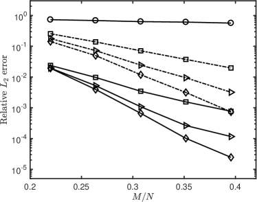
Figure 1: Results for the ridge function. “$\circ$”: standard $\ell_{1}$, “$\square$”: $\ell_{1}$ with 3 rotations, “$\triangleright$”: $\ell_{1}$ with 6 rotations, “$\diamond$”: $\ell_{1}$ with 9 rotations. Dash lines result from using initial guess of $\mathbf{A}$ based on compressive sensing results (Algorithm 3), while solid lines are results using an initial guess of $\mathbf{A}$ from SIR (Algorithm 4)

.

4.2 Function with high compressibility

Consider the following function:

$$u(\bm{\xi})=\sum_{|\bm{\alpha}|=0}^{P}c_{\bm{\alpha}}\psi_{\bm{\alpha}}(\bm{\xi})=\sum_{n=1}^{N}c_{n}\psi_{n}(\bm{\xi}),\quad\bm{\xi}=(\xi_{1},\xi_{2},\cdots,\xi_{d}),$$ (21)

where, $\psi_{\bm{\alpha}}$ are normalized multivariate Hermite polynomials, $d=20,P=3,N=1771$, and the coefficients $c_{n}$ are chosen as uniformly distributed random numbers,

$$c_{n}=\zeta/n^{1.5},\quad\zeta\sim\mathcal{U}[-1,1].$$ (22)

For this example, we generate $N$ samples of $\zeta$: $\zeta^{1},\zeta^{2},\cdots,\zeta^{N}$, and then divide them by $n^{1.5},n=1,2,\cdots,N$ to obtain a random “compressible signal” $\bm{c}$. This example is also used in [56, 58] to demonstrate the effectiveness of the rotational $\ell_{1}$ method. The dimension is increased to $d=20$ in this test. The function $u$ is not exactly sparse before or after rotation. This is reflected in the right plot in Fig. 2, which shows the eigenvalues of $\mathbf{G}$. These eigenvalues indicate that all subspaces identified by eigen-decomposition of $\mathbf{G}$ make contributions to $u$, although some of them are quite insignificant. The left plot in Fig. 2 shows results obtained by applying Algorithm 3 and Algorithm 4 with re-weighted $\ell_{1}$ minimization and compares them with the standard $\ell_{1}$ and re-weighted $\ell_{1}$ methods. Apparently, the ADM algorithm improves the accuracy, and SIR provides a better initial guess of $\mathbf{A}$, especially when $M/N$ is very small, i.e., when the available data are very limited. We also notice that as $M$ increases, the advantage of the SIR-based ADM method decreases. When $M=110$ ($M/N\approx 0.062$), the SIR-based ADM (Algorithm 4) is slightly less accurate than the ADM method (Algorithm 3). This is because the size $M$ is sufficient to compute a $u_{g}$ that can yield a slightly better initial guess of $\mathbf{A}$ using the gradient information than SIR.

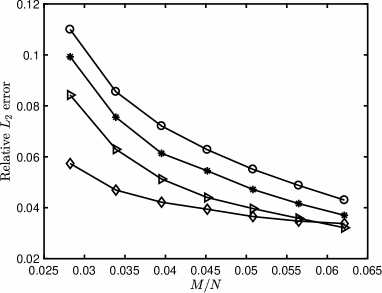
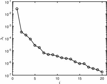
Figure 2: Results for the highly compressible function. Left: relative $L_{2}$ error. “$\circ$”: standard $\ell_{1}$, “$\ast$”: re-weighted $\ell_{1}$, “$\triangleright$”: ADM, “$\diamond$”: SADM. Right: eigenvalues of matrix $G$.

4.3 Korteweg-de Vries equation

As an example application of the new method to a nonlinear differential equation, we consider the Korteweg-de Vries (KdV) equation with time-dependent additive noise [32]:

$$u_{t}(x,t;\bm{\xi})-6u(x,t;\bm{\xi})u_{x}(x,t;\bm{\xi})+u_{xxx}(x,t;\bm{\xi})=f(t;\bm{\xi}),\quad x\in(-\infty,\infty),$$ (23)

$$u(x,0;\bm{\xi})=-2\operatorname{sech}^{2}(x).$$

We model $f(t;\bm{\xi})$ as a random field represented by the following Karhuen-Loève (KL) expansion:

$$f(t;\bm{\xi})=\sigma\sum_{i=1}^{d}\sqrt{\lambda_{i}}\phi_{i}(t)\xi_{i},$$ (24)

where $\sigma$ is a constant and $\{\lambda_{i},\phi_{i}(t)\}_{i=1}^{d}$ are eigenpairs of the exponential covariance kernel

$$C(t,t^{\prime})=\exp\left(-\dfrac{|t-t^{\prime}|}{l_{c}}\right).$$

The explicit form of $\lambda_{i}$ and $\phi_{i}$ can be found in [19]. In this problem, we set $l_{c}=0.1$ and $d=100$ ($\sum_{i=1}^{d}\lambda_{i}>0.978\sum_{i=1}^{\infty}\lambda_{i}$). In this case, the exact one-soliton solution is

$$\begin{split}u(x,t;\bm{\xi})=&\sigma\sum_{i=1}^{d}\sqrt{\lambda_{i}}\xi_{i}\int_{0}^{t}\phi_{i}(y)\mathrm{d}y\\ &-2\operatorname{sech}^{2}\left(x-4t+6\sigma\sum_{i=1}^{d}\sqrt{\lambda_{i}}\xi_{i}\int_{0}^{t}\int_{0}^{z}\phi_{i}(y)\mathrm{d}y\mathrm{d}z\right).\end{split}$$ (25)

The QoI is chosen to be $u(x,t;\bm{\xi})$ at $x=6,t=1$ with $\sigma=0.4$. Because an analytical expression for $\phi_{i}$ is available, we can compute the integrals in Eq. (25) with high accuracy. Denoting

$$A_{i}=\sqrt{\lambda_{i}}\int_{0}^{1}\phi_{i}(y)\mathrm{d}y,\quad B_{i}=\sqrt{\lambda_{i}}\int_{0}^{1}\int_{0}^{z}\phi_{i}(y)\mathrm{d}y\mathrm{d}z,\quad i=1,2,\cdots,d,$$ (26)

the analytical solution is

$$u(x,t;\bm{\xi})\big{|}_{x=6,t=1}=\sigma\sum_{i=1}^{d}A_{i}\xi_{i}-2\operatorname{sech}^{2}\left(2+6\sigma\sum_{i=1}^{d}B_{i}\xi_{i}\right).$$ (27)

We set $P=2$ ($N=5151$) to construct $u_{g}$ using re-weighted $\ell_{1}$ minimization and set $\tilde{d}=12$ and $P=3$ ($N=455$) to construct $\tilde{u}_{g}$ using SADMDR (Algorithm 5). The relative error of the mean and standard deviation obtained from ADM, SADMDR, and the MC method with $M$ realizations, compared with the reference solution, are presented in Fig. 3. For the estimate of mean, both re-weighted $\ell_{1}$ and SADMDR are more accurate than MC, and the SADMDR is up to $30\%$ more accurate than re-weighted $\ell_{1}$ for small $M$. The accuracy of ADM and SADMDR becomes similar as $M$ increases. For the estimate of the standard deviation, the advantage of SADMDR over ADM is much more distinct: for all considered $M$, SADMDR has a $50\%$ smaller error than MC, while the re-weighted $\ell_{1}$ method has a similar error as MC for small $M$ (error of re-weighted $\ell_{1}$ is slightly larger than in MC for $M=160$) and $20\%$ smaller error than MC for larger $M$. Again, the observed difference between the re-weighted $\ell_{1}$ and SADMDR results become smaller as $M$ increases.

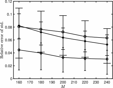
Figure 3: Results for the Korteweg-de Vries equation. Left: relative error of mean; Right: relative error of standard deviation. “$\circ$”: direct estimate from Monte Carlo samples; “$\ast$”: re-weighted $\ell_{1}$; “$\diamond$”: SADMDR. “ ”: quantiles of direct estimate from Monte Carlo samples; “ ”: quantiles of re-weighted $\ell_{1}$; “ ”: quantiles of SADMDR.

Moreover, the results obtained from Algorithm 3 and Algorithm 4 are almost the same as the re-weighted $\ell_{1}$ results, so the results are not plotted. This implies that the rotations identified in the iteration by the gradient of $u$ approximated from $u_{g}$ with up to second-order Hermite polynomials are not sufficiently informative to provide good guidance for a sparser representation–no matter what initial guess is used. In [56], the KdV equation with $12$ random parameters is solved using a $u_{g}$ approximation with $P=4$. In that example, Algorithm 3 reduced the relative $L_{2}$ error of re-weighted $\ell_{1}$ by up to $75\%$. This implies that higher-order terms in the Hermite polynomial expansion are important for determining the rotation matrix. In the KdV equation used in this work, $d=100$, and $M$ is small. Thus, there are not enough samples to compute terms even in $P=3$ gPC expansion without first reducing the dimensionality $d$. We use SIR to set reduced dimension $\tilde{d}=12$. Then, we choose $P=3$ to include as many terms as possible in the Hermite polynomial expansion but still keep the number of unknowns in a reasonable range ($N=455$).

4.4 Groundwater flow

Next, we consider a model that simulates the groundwater flow in a confined aquifer, which spans a $2000$ m $\times 1000$ m area [30]. The north and south boundaries of the aquifer are two rivers with constant but different hydraulic heads, whereas the east and west boundaries are bounded by no-flow conditions. This model can be described by the following equations:

$$\begin{cases}q(x,y)=-T(x,y)\nabla u(x,y),\quad(x,y)\in D=[0,2000]\times[0,1000]\\ \nabla\cdot q(x,y)=0,\end{cases}$$ (28)

and boundary conditions

$$\begin{cases}u(x,0)=0,~{}u(x,1000)=10,\\ q_{x}(0,y)=q_{x}(2000,y)=0,\end{cases}$$ (29)

where $u$ is hydraulic head $[\text{m}]$, $T$ is transmissivity $[\text{m}^{2}/\text{day}]$, and $\bm{q}=(q_{x},q_{y})^{\mathsf{T}}$ is flux vector $[m^{2}/\text{day}]$. The QoI is the hydraulic head at a specific location: $u^{*}=u(200,500)$. The equations are solved by the finite difference method on a $61\times 31$ computational grid. The transmissivity $T(x,y)$ is described by log-normal random field $T(x,y)=\ln S(x,y)$, where $S$ satisfies: 1) for $(x,y)\in D$, $S(x,y)\sim\mathcal{N}(2,1)$; 2) for $(x,y),(x^{\prime},y^{\prime})\in D$, the covariance kernel is

$$C(x,y;x^{\prime},y^{\prime})=\exp\left(-\dfrac{|x-x^{\prime}|}{l_{x}}-\dfrac{|y-y^{\prime}|}{l_{y}}\right).$$

In this problem, we set $l_{x}=l_{y}=300$, and $S(x,y)$ is represented by a KL-expansion with $100$ terms ($\sum_{i=1}^{100}\lambda_{i}>0.85\sum_{i=1}^{\infty}\lambda_{i}$). We set $P=2$ ($N=5151$) to construct $u_{g}$ using the re-weighted $\ell_{1}$ method and set $\tilde{d}=20$ and $P=3$ ($N=1771$) to construct $\tilde{u}_{g}$ using SADMDR (Algorithm 5). Figure 4 represents the relative error of mean and standard deviation estimates. For the mean, both methods exhibit better accuracy than direct estimation from MC with the same number of sampling points. The re-weighted $\ell_{1}$ method reduces the relative error by up to $30\%$ compared with MC, and the SADMDR reduces the relative error by up to $50\%$. For the standard deviation, re-weighted $\ell_{1}$ has relative error that is several times larger than the error of MC for all considered $M$. On the other hand, SADMDR reduces the error of MC by approximately $45\%$ for $M>160$. For $M=140$, SADMDR performs worse than MC because the sample size is too small for this high-dimensional ($d=100$) problem.

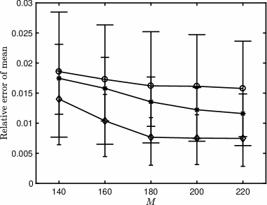
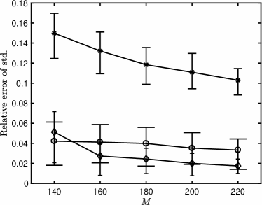
Figure 4: Results for the groundwater flow. Left: relative error of mean; Right: relative error of standard deviation. “$\circ$”: direct estimate from Monte Carlo samples; “$\ast$”: re-weighted $\ell_{1}$; “$\diamond$”: SADMDR. “ ”: quantiles of direct estimate from Monte Carlo samples; “ ”: quantiles of re-weighted $\ell_{1}$; “ ”: quantiles of SADMDR.

Again, the Algorithms 3 and 4 results are not presented as they are almost the same as those by re-weighted $\ell_{1}$. This example also demonstrates that reducing dimension and increasing $P$ while keeping $N$ in a reasonable range for compressive sensing is important for an accurate approximation of $u$.

4.5 High-dimensional function

In the final example, we demonstrate the ability of SADMDR to deal with very high-dimensional problems. Specifically, we consider the following function [21]:

$$u(\bm{\xi})=\exp\left(2-\sum_{i=1}^{d}\dfrac{\sin(i)\xi_{i}}{i}\right),\quad d=500.$$ (30)

We use a third-order gPC expansion without interaction terms, i.e., we only use constant and $\{\xi_{i},(\xi_{i}^{2}-1)/\sqrt{2},(\xi_{i}^{3}-3\xi_{i})/\sqrt{6}\}_{i=1}^{d}$ as basis functions ($N=1+500+500=1001$), to construct $u_{g}$ using the re-weighted $\ell_{1}$ method, then we set $\tilde{d}=20$ and $P=3$ ($N=1771$) to construct $\tilde{u}_{g}$ using SADMDR (Algorithm 5). The relative errors of the mean and standard deviation are presented in Fig. 5. As before, SADMDR reduces the error in the mean prediction by $40\%$ compared with MC. The $u_{g}$ by re-weighted $\ell_{1}$ provide a similar error in the estimate of mean as MC. For the standard deviation estimate, the error in re-weighted $\ell_{1}$ is approximately $10\%$ smaller than $MC$, while SADMDR has approximately $30\%$ smaller error than in MC. More importantly, unlike previous examples where the differences between re-weighted $\ell_{1}$ and SADMDR became smaller quickly with increasing $M$, in this case, the accuracy of SADMDR relative to re-weighted $\ell_{1}$ changes slowly in the range of studied $M$. This is because the dimension of the problem is very high, and dimension reduction is more critical than in the previous examples.

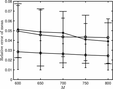
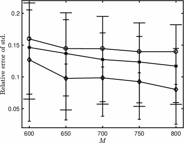
Figure 5: Results for the high-dimensional function. “$\circ$”: direct estimate from Monte Carlo samples; “$\ast$”: re-weighted $\ell_{1}$; “$\diamond$”: SADMDR. “ ”: quantiles of direct estimate from Monte Carlo samples; “ ”: quantiles of re-weighted $\ell_{1}$; “ ”: quantiles of SADMDR.

The ADM and SADM algorithms fail to improve the accuracy in this example as in Examples 3 and 4, because the dimension is very high and the available data are too limited for these two approaches.

4.6 Discussion

The rotation matrix computed from $\mathbf{G}$ in Eq. (15) was used for dimension reduction in active subspace method [39, 12]. We can also use it to replace SIR in Algorithm 5. Specifically, on computing the eigen-decomposition of $\mathbf{G}$ based on the $u_{g}$ from Algorithms 1 or 3, we can construct $\hat{\mathbf{A}}$ that consists of eigenvectors corresponding to the $\tilde{d}$ largest eigenvalues, where $\tilde{d}<d$ is the reduced dimension. Then we project $\bm{\xi}$ to $\tilde{\bm{\xi}}=\hat{\mathbf{A}}\bm{\xi}$, and run step 4 in Algorithm 5 to construct a surrogate model. Apparently, the accuracy of estimating $\nabla u$ is critical to the dimension reduction. Since we do not have samples of $\nabla u$, we have to approximate $\nabla u$ from $\nabla u_{g}$. Therefore one can roughly expect that an accurate $u_{g}$ yields better performance of dimension reduction, while a less accurate $u_{g}$ results in worse performance. We use the KdV equation in Example 3 as a demonstration. As we presented in Example 3, we set $P=2$ ($N=5151$) to construct $u_{g}$ using re-weighted $\ell_{1}$ minimization. Then we approximate $\mathbf{G}$ based on $u_{g}$, and truncate the dimension to $\tilde{d}=12$. Next, we set $P=3$ ($N=455$), and construct $\tilde{u}_{g}^{W}$ using ADM method. We compare the accuracy of this $\tilde{u}_{g}^{W}$ with $u_{g}$ and $\tilde{u}_{g}$ (from SADMDR by setting $\tilde{d}=12$) in Example 3 and present the results in Fig. 6. When $M<200$, $\tilde{u}_{g}$ is more accurate in estimating mean than $u_{g}$ and $u_{g}^{W}$. But when $M\geq 200$, $\tilde{u}_{g}^{W}$ is the best for estimating the mean. For the estimate of the standard deviation, $\tilde{u}_{g}$ is always the best in the range of $M$ we chose. But the difference between $\tilde{u}_{g}$ and $\tilde{u}_{g}^{W}$ decays as $M$ increases. These phenomena are similar to those in Example 2. Again, this is because as $M$ increases, $\ell_{1}$ or re-weighted $\ell_{1}$ minimization is able to provide more accurate estimate of $u_{g}$, and consequently more accurate estimates of $\nabla u$ and $\mathbf{G}$. Therefore, the initial guess of $\mathbf{A}$ (Example 2) or $\hat{\mathbf{A}}$ (this example) becomes better, and finally exceeds the one estimated from SIR when $M$ is sufficiently large. An approach using Algorithm 3 to estimate $\mathbf{G}$, then perform dimension reduction was proposed in [53]. It worked well for specific problems in that study. As we show in Example 2 and this comparison, there is no guarantee that SIR works better than the gradient-based method for dimension reduction for any $M$. If the gradient information is not available, or it is difficult to approximate the gradient accurately, SIR can be a good choice. In practice, if no prior knowledge of the QoI is available, users may construct different surrogate models, then use model selection tools (e.g., AIC [2], BIC [41] or cross validation [26]) to decide which method to employ.

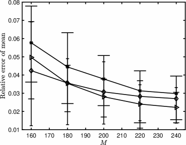
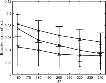
Figure 6: Results for the high-dimensional function. “$\ast$”: re-weighted $\ell_{1}$; “$\rhd$” dimension reduction based on re-weight $\ell_{1}$;“$\diamond$”: SADMDR. “ ”: quantiles of re-weighted $\ell_{1}$ ($u_{g}$); “ ”: quantiles of gradient-based dimension reduction ($\tilde{u}_{g}^{W}$); “ ”: quantiles of SADMDR ($\tilde{u}_{g}$).

5 Conclusions

We use the sliced inverse regression method to provide a better initial guess for the alternating direction method proposed in [56], which enhances the sparsity of the Hermite polynomial expansion of the QoI relying on i.i.d. Gaussian random variables. The enhancement of sparsity helps the compressive sensing method to obtain a more accurate Hermite polynomial expansion. Examples 1 and 2 show that when the available data (e.g., the number of model realizations, $M$) are limited (compared with the number of unknown terms in the QoI expansion), the compressive sensing method with the initial guess provided by SIR can yield more accurate results than the standard $\ell_{1}$ minimization (or re-weighted $\ell_{1}$) used in [56]. We also demonstrate that when the problem dimensionality is very high and the available data size is small, we can first use SIR to perform dimension reduction then use the ADM method based on the reduced system to approximate the mean and standard deviation of the QoI more accurately. The dimension reduction allows for inclusion of more higher-order terms in the Hermite polynomial expansion of the QoI. Consequently, more information related to variance and other higher-order terms are included in the expansion. This is illustrated in Examples 3-5 where the improvement in the estimate of standard deviation is much more significant than in the estimate of the mean. We demonstrate the advantage of the new algorithms (i.e., Algorithms 4 and 5) when the number of samples is much smaller than the number of terms in the QoI expansion and is far below the requirement of the sample size for the $\ell_{1}$ minimization. Examples 1 and 2 (relatively low-dimensional problems) demonstrate that the accuracy of the ADM method (i.e., Algorithm 3) improves with increasing $M$ and it can be as good as or even better than the SIR-aided method for larger $M$. In Examples 3-5 (higher-dimensional problems), $\ell_{1}$ minimization without dimension reduction does not work well for relatively small $M$. However, if we dramatically increase $M$, it is expected that the accuracy of ADM will be comparable to that of SIR-aided ADM methods.

In this work, the rotation matrix is obtained in two different ways. SIR uses conditional mean to identify the matrix $\hat{A}$, while in ADM, the gradient of $u$ is used to iteratively identify the rotation. Both approaches have been widely used in statistics algorithms for dimension reduction. Notably, other approaches also can be incorporated in our algorithm. For example, different methods for sufficient dimension reduction (e.g., [29, 24]) may provide a better initial guess of the rotation matrix or better dimension reduction strategy for specific problems. In each iteration, the rotation can be obtained from these SIR-type methods instead of using the gradient information. Also, when $d$ is not very large (typically $d<100$), Algorithm 3 or Algorithm 4 can be used to obtain $u_{g}$ then construct the gradient matrix $\mathbf{G}$ of $u$ and reduce the dimension according to the magnitude of eigenvalues of $\mathbf{G}$ [53].

Moreover, we demonstrate the effectiveness of ADM for $\ell_{1}$ minimization. ADM can also be integrated with other optimization methods to solve the compressive sensing problem, e.g., OMP [6], $\ell_{1-2}$ minimization [59], etc. Further, it could be advantageous to integrate our method with sampling strategies (e.g., [3, 4]), basis selection method (e.g., [23]), or Bayesian approach (e.g., [25]). The combination of these methods can be especially useful for problems where experiments or simulations are costly and where a good surrogate model of the QoI is needed, e.g., in inverse problems based on a Bayesian framework ([40, 57]).

Finally, as discussed in Section 3, a correct balance between the reduced dimension $\tilde{d}$ and the selection of high-order terms in the expansion can yield a more accurate approximation of the QoI. The theoretical analysis on SIR-type dimension reduction methods can be found in [29, 24], which help to identify $\tilde{d}$. After $\tilde{d}$ is set, model selection techniques can be used to select the polynomial order $P$. In practice, whether to use dimension reduction depends on the available data size, model complexity and property of QoI. Again, model selection tools can be used to identify a suitable surrogate model when no prior knowledge is available.

Appendix

A. Cross-validation method

The algorithm in [16] is used to estimate the error term $\epsilon$ in $(P_{1,\epsilon})$. This algorithm is summarized in Algorithm 6.

Algorithm 6 Cross-validation to estimate the error $\epsilon$.

1:  Divide the $M$ output samples to $M_{r}$ reconstruction ($\bm{u}_{r}$) and $M_{v}$ validation ($\bm{u}_{v}$) samples and divide the measurement matrix $\mathbf{\Psi}$ correspondingly into $\mathbf{\Psi}_{r}$ and $\mathbf{\Psi}_{v}$.

2:  Choose multiple values for $\epsilon_{r}$ such that the exact error $\|\mathbf{\Psi}_{r}\bm{c}-\bm{u}_{r}\|_{2}$ of the reconstruction samples is within the range of $\epsilon_{r}$ values.

3:  For each $\epsilon_{r}$, solve $(P_{1,\epsilon})$ with $\bm{u}_{r}$ and $\mathbf{\Psi}_{r}$ to obtain $\hat{\bm{c}}$. Then compute $\epsilon_{v}=\|\mathbf{\Psi}_{v}\hat{\bm{c}}-\bm{u}_{v}\|_{2}$.

4:  Find the minimum value of $\epsilon_{v}$ and its corresponding $\epsilon_{r}$. Set $\epsilon=\sqrt{M/M_{r}}\epsilon_{r}$.

Of note, a technique to avoid the cross-validation step in some cases is proposed in [1],.

Ackowledgement

This work was supported by the U.S. Department of Energy (DOE), Office of Science, Office of Advanced Scientific Computing Research (ASCR) as part of the Multifaceted Mathematics for Complex Systems project and the Uncertainty Quantification in Advection-Diffusion-Reaction Systems projects. A portion of the research described in this paper was conducted under the Laboratory Directed Research and Development Program at Pacific Northwest National Laboratory (PNNL). PNNL is operated by Battelle for the DOE under Contract DE-AC05-76RL01830.

References

- [1] Ben Adcock. Infinite-dimensional compressed sensing and function interpolation. Found. Comput. Math., pages 1–41, 2017.
- [2] Hirotugu Akaike. A new look at the statistical model identification. IEEE Trans. Automat. Contr., 19(6):716–723, 1974.
- [3] Negin Alemazkoor and Hadi Meidani. Divide and conquer: An incremental sparsity promoting compressive sampling approach for polynomial chaos expansions. Comput. Methods in Appl. Mech. and Eng., 318:937–956, 2017.
- [4] Negin Alemazkoor and Hadi Meidani. A near-optimal sampling strategy for sparse recovery of polynomial chaos expansions. arXiv preprint arXiv:1702.07830, 2017.
- [5] Ivo Babuška, Fabio Nobile, and Raul Tempone. A stochastic collocation method for elliptic partial differential equations with random input data. SIAM Rev., 52(2):317–355, 2010.
- [6] Alfred M. Bruckstein, David L. Donoho, and Michael Elad. From sparse solutions of systems of equations to sparse modeling of signals and images. SIAM Rev., 51(1):34–81, 2009.
- [7] Robert H Cameron and William T Martin. The orthogonal development of non-linear functionals in series of fourier-hermite functionals. Ann. Math., pages 385–392, 1947.
- [8] Emmanuel J. Candès. The restricted isometry property and its implications for compressed sensing. C. R. Math. Acad. Sci. Paris, 346(9-10):589–592, 2008.
- [9] Emmanuel J Candès, Justin K Romberg, and Terence Tao. Stable signal recovery from incomplete and inaccurate measurements. Comm. Pure Applied Math., 59(8):1207–1223, 2006.
- [10] Emmanuel J. Candès and Terence Tao. Decoding by linear programming. IEEE Trans. Inform. Theory, 51(12):4203–4215, 2005.
- [11] Emmanuel J. Candès, Michael B. Wakin, and Stephen P. Boyd. Enhancing sparsity by reweighted minimization. J. Fourier Anal. Appl., 14(5-6):877–905, 2008.
- [12] Paul G Constantine, Eric Dow, and Qiqi Wang. Active subspace methods in theory and practice: Applications to kriging surfaces. SIAM J. Sci. Comput., 36(4):A1500–A1524, 2014.
- [13] R Dennis Cook and Sanford Weisberg. Sliced inverse regression for dimension reduction: Comment. J. Am. Stat. Assoc., 86(414):328–332, 1991.
- [14] David L Donoho. Compressed sensing. IEEE Trans. Inform. Theory, 52(4):1289–1306, 2006.
- [15] David L. Donoho, Michael Elad, and Vladimir N. Temlyakov. Stable recovery of sparse overcomplete representations in the presence of noise. IEEE Trans. Inform. Theory, 52(1):6–18, 2006.
- [16] Alireza Doostan and Houman Owhadi. A non-adapted sparse approximation of PDEs with stochastic inputs. J. Comput. Phys., 230(8):3015–3034, 2011.
- [17] Oliver G Ernst, Antje Mugler, Hans-Jörg Starkloff, and Elisabeth Ullmann. On the convergence of generalized polynomial chaos expansions. ESAIM: Math. Model. Num. Anal., 46(2):317–339, 2012.
- [18] Jasmine Foo, Xiaoliang Wan, and George Em Karniadakis. The multi-element probabilistic collocation method (ME-PCM): error analysis and applications. J. Comput. Phys., 227(22):9572–9595, 2008.
- [19] Roger G. Ghanem and Pol D. Spanos. Stochastic finite elements: a spectral approach. Springer-Verlag, New York, 1991.
- [20] Jerrad Hampton and Alireza Doostan. Compressive sampling of polynomial chaos expansions: Convergence analysis and sampling strategies. J. Comput. Phys., 280(0):363–386, 2015.
- [21] Jerrad Hampton and Alireza Doostan. Basis adaptive sample efficient polynomial chaos (base-pc). Journal of Computational Physics, 371:20–49, 2018.
- [22] James William Hardin and Joseph Hilbe. Generalized linear models and extensions. Stata Press, 2007.
- [23] John D Jakeman, Michael S Eldred, and Khachik Sargsyan. Enhancing -minimization estimates of polynomial chaos expansions using basis selection. J. Comput. Phys., 289:18–34, 2015.
- [24] Bo Jiang, Jun S Liu, et al. Variable selection for general index models via sliced inverse regression. Ann. Stat., 42(5):1751–1786, 2014.
- [25] Georgios Karagiannis, Bledar A Konomi, and Guang Lin. A Bayesian mixed shrinkage prior procedure for spatial–stochastic basis selection and evaluation of gpc expansions: Applications to elliptic spdes. J. Comput. Phys., 284:528–546, 2015.
- [26] Ron Kohavi et al. A study of cross-validation and bootstrap for accuracy estimation and model selection. In Ijcai, volume 14, pages 1137–1145. Stanford, CA, 1995.
- [27] Huan Lei, Xiu Yang, Bin Zheng, Guang Lin, and Nathan A Baker. Constructing surrogate models of complex systems with enhanced sparsity: quantifying the influence of conformational uncertainty in biomolecular solvation. SIAM Multiscale Model. Simul., 13(4):1327–1353, 2015.
- [28] Ker-Chau Li. Sliced inverse regression for dimension reduction. J. Am. Stat. Assoc., 86(414):316–327, 1991.
- [29] Lexin Li. Sparse sufficient dimension reduction. Biometrika, 94(3):603–613, 2007.
- [30] Weixuan Li, Guang Lin, and Bing Li. Inverse regression-based uncertainty quantification algorithms for high-dimensional models: Theory and practice. J. Comput. Phys., 321:259–278, 2016.
- [31] Yiou Li, Mihai Anitescu, Oleg Roderick, and Fred Hickernell. Orthogonal bases for polynomial regression with derivative information in uncertainty quantification. Int. J. Uncertain. Quant., 1(4), 2011.
- [32] Guang Lin, Leopold Grinberg, and George Em Karniadakis. Numerical studies of the stochastic Korteweg-de Vries equation. J. Comput. Phys., 213(2):676–703, 2006.
- [33] D. Needell. Noisy signal recovery via iterative reweighted minimization. In Proc. Asilomar Conf. on Signal Systems and Computers, Pacific Grove, CA, 2009.
- [34] Ji Peng, Jerrad Hampton, and Alireza Doostan. A weighted -minimization approach for sparse polynomial chaos expansions. J. Comput. Phys., 267(0):92–111, 2014.
- [35] Ji Peng, Jerrad Hampton, and Alireza Doostan. On polynomial chaos expansion via gradient-enhanced -minimization. J. Comput. Phys., 310:440–458, 2016.
- [36] Holger Rauhut and Rachel Ward. Sparse legendre expansions via -minimization. J. Approx. Theory, 164(5):517–533, 2012.
- [37] Holger Rauhut and Rachel Ward. Interpolation via weighted minimization. Appl. Comput. Harmon. Anal., 40(2):321–351, 2016.
- [38] Mark Rudelson and Roman Vershynin. On sparse reconstruction from Fourier and Gaussian measurements. Comm. Pure Appl. Math., 61(8):1025–1045, 2008.
- [39] Trent Michael Russi. Uncertainty quantification with experimental data and complex system models. PhD thesis, UC Berkeley, 2010.
- [40] Khachik Sargsyan, Cosmin Safta, Habib N Najm, Bert J Debusschere, Daniel Ricciuto, and Peter Thornton. Dimensionality reduction for complex models via Bayesian compressive sensing. Int. J. Uncertain. Quant., 4(1), 2014.
- [41] Gideon Schwarz et al. Estimating the dimension of a model. Ann. Stat., 6(2):461–464, 1978.
- [42] S. Smolyak. Quadrature and interpolation formulas for tensor products of certain classes of functions. Sov. Math. Dokl., 4:240–243, 1963.
- [43] Menner A Tatang, Wenwei Pan, Ronald G Prinn, and Gregory J McRae. An efficient method for parametric uncertainty analysis of numerical geophysical models. J. Geophys. Res-Atmos. (1984–2012), 102(D18):21925–21932, 1997.
- [44] Ramakrishna Tipireddy and Roger Ghanem. Basis adaptation in homogeneous chaos spaces. J. Comput. Phys., 259(0):304–317, 2014.
- [45] E. van den Berg and M. P. Friedlander. SPGL1: A solver for large-scale sparse reconstruction, June 2007. http://www.cs.ubc.ca/labs/scl/spgl1.
- [46] E. van den Berg and M. P. Friedlander. Probing the Pareto frontier for basis pursuit solutions. SIAM J. Sci. Comput., 31(2):890–912, 2008.
- [47] Sanford Weisberg et al. Dimension reduction regression in R. J. Stat. Softw., 7(1):1–22, 2002.
- [48] Yingcun Xia. A constructive approach to the estimation of dimension reduction directions. Ann. Stat., pages 2654–2690, 2007.
- [49] Yingcun Xia, Howell Tong, WK Li, and Li-Xing Zhu. An adaptive estimation of dimension reduction space. J. Roy. Stat. Soc. B, 64(3):363–410, 2002.
- [50] Dongbin Xiu and Jan S. Hesthaven. High-order collocation methods for differential equations with random inputs. SIAM J. Sci. Comput., 27(3):1118–1139, 2005.
- [51] Dongbin Xiu and George Em Karniadakis. The Wiener-Askey polynomial chaos for stochastic differential equations. SIAM J. Sci. Comput., 24(2):619–644, 2002.
- [52] Liang Yan, Ling Guo, and Dongbin Xiu. Stochastic collocation algorithms using -minimization. Int. J. Uncertain. Quant., 2(3):279–293, 2012.
- [53] Xiu Yang, David A Barajas-Solano, William S Rosenthal, and Alexandre M Tartakovsky. PDF estimation for power grid systems via sparse regression. arXiv preprint arXiv:1708.08378, 2017.
- [54] Xiu Yang, Minseok Choi, Guang Lin, and George Em Karniadakis. Adaptive ANOVA decomposition of stochastic incompressible and compressible flows. J. Comput. Phys., 231(4):1587–1614, 2012.
- [55] Xiu Yang and George Em Karniadakis. Reweighted minimization method for stochastic elliptic differential equations. J. Comput. Phys., 248(1):87–108, 2013.
- [56] Xiu Yang, Huan Lei, Nathan Baker, and Guang Lin. Enhancing sparsity of hermite polynomial expansions by iterative rotations. J. Comput. Phys., 307:94–109, 2016.
- [57] Xiu Yang, Huan Lei, Peiyuan Gao, Dennis G Thomas, David L Mobley, and Nathan A Baker. Atomic radius and charge parameter uncertainty in biomolecular solvation energy calculations. J. Chem. Theory Comput., 14(2):759–767, 2018.
- [58] Xiu Yang, Xiaoliang Wan, and Lin Lin. A general framework for enhancing sparity of generalized polynomial chaos expansions. arXiv preprint arXiv:1707.02688, 2017.
- [59] Penghang Yin, Yifei Lou, Qi He, and Jack Xin. Minimization of 1-2 for compressed sensing. SIAM J. Sci. Comput., 37(1):A536–A563, 2015.
- [60] Zheng Zhang, Xiu Yang, Giovanni Marucci, Paolo Maffezzoni, Ibrahim Abe Elfadel, George Karniadakis, and Luca Daniel. Stochastic testing simulator for integrated circuits and MEMS: Hierarchical and sparse techniques. In 2014 IEEE Proc. Custom Int. Circ. Con. (CICC), pages 1–8, Sept 2014.