Non-local Coulomb interactions on the triangular lattice in the high-doping regime: Spectra and charge dynamics from Extended Dynamical Mean Field Theory

Abstract

We explore the two-dimensional extended Hubbard model on the triangular lattice in the high doping regime. On-site and nearest-neighbour repulsive interactions are treated in a non-perturbative way by means of Extended Dynamical Mean Field Theory. We compute the low-temperature phase diagram, displaying a metallic phase and a symmetry-broken phase for strong intersite repulsions. We describe the correlation effects on both single-particle and two-particle observables in the metallic phase. Whereas single-particle spectra feature a Hubbard satellite typical of strongly correlated systems, local susceptibilities remain close to their non-interacting limit, even for large on-site repulsions. We argue that this behaviour is typical of the strongly doped case. We also report a region in parameter space with negative static local screening.

Transition metal oxides display a wide variety of exotic phenomena as a function of the filling of the $d$-shell. Cuprates are the most popular example, going from a Mott-insulating phase to a charge-density wave to a superconductor to a metal Imada et al. (1998). A similar phenomenology is realized for materials on the triangular lattice, such as sodium-doped cobaltates, Na_xCoO₂, where properties such as superconductivity Takada et al. (2003) or a high thermoelectric power Terasaki et al. (1997) can be tuned with doping. An accurate description of materials away from the half-filled limit is thus important.

On the triangular lattice at incommensurate filling, charge dynamics can lead to a variety of exotic phases Tocchio et al. (2014). Their intriguing properties originate from the interplay between local and non-local interaction parameters, as well as quantum hopping. Specifically, a phase exhibiting simultaneously charge-order and metallicity Tocchio et al. (2014) in the extended Hubbard model is reminiscent of the pinball liquid for spinless fermions Hotta and Furukawa (2006, 2007), or the supersolid for hard-core bosons Wessel and Troyer (2005); Heidarian and Damle (2005); Melko et al. (2005); Zhang et al. (2011), where the particles segregate between mobile and frozen. Understanding such phases is not only of purely academic interest, but also helps to describe actual materials more accurately. An anisotropic extended Hubbard model was used to describe charge-ordering in $\theta$-(BEDT-TTF)₂X Cano-Cortés et al. (2011). Multiorbital effects were shown to enrich again the phase diagram (relevant for materials with $e_{g}$ orbitals) Février et al. (2015). The possibility of charge instabilities originating from the microscopic details of the hopping processes within a 3-orbital system was described in Ref. Koshibae and Maekawa, 2003. Quite generally, it is expected that charge excitations and screening play a key role in the doped triangular lattice.

The development of many-body techniques that are able to describe the physics of charge-ordering and screening, induced by long-range Coulomb interactions in strongly correlated electron materials, has become an active topic in condensed matter theory in recent years. Extended Dynamical Mean Field Theory (EDMFT) Sengupta and Georges (1995); Kajueter (1996); Si and Smith (1996) widens the scope of Dynamical Mean Field Theory (DMFT) (for a review, see Ref. Georges et al., 1996) to systems with non-local interactions. In this method, the lattice model is mapped onto an effective local impurity problem with frequency-dependent effective local interactions, that are related self-consistently to the local polarization function. Following the development of improved Quantum Monte Carlo algorithms suitable for solving impurity models with frequency-dependent interactions, several works presenting fully self-consistent EDMFT implementations have appeared over the last few years (see e.g. Refs Ayral et al., 2012, 2013; Huang et al., 2014; van Loon et al., 2014; Hafermann et al., 2014; van Loon et al., 2015; Ayral et al., 2017). In a recent realistic study Nomura et al. (2016) this theory was used to determine the phase diagram of alcali-doped fullerides. Ref. Rademaker et al., 2015 investigated glassy behavior, possibly relevant for organic materials. Finally, Ref. Camjayi et al., 2008 presented a DMFT study of the Wigner-Mott transition on the triangular lattice.

Combined many-body perturbation theory + dynamical mean field theory (“$GW$+DMFT”) Biermann et al. (2003); Sun and Kotliar (2004); Ayral et al. (2012, 2013); Biermann (2014) goes beyond the local description of screening by including the non-local polarization at the level of the random phase approximation. The dual boson scheme Rubtsov et al. (2012); van Loon et al. (2014); Stepanov et al. (2016a) introduces non-local corrections beyond $GW$+DMFT, thereby curing artefacts of the plasmon dispersion present in the simpler schemes. Most work so far has however focussed on systems on the square lattice, and much less is known for triangular lattice models (see however Refs Hansmann et al., 2013, 2016).

In this study, we explore single-particle properties and screening in an extended Hubbard model on the triangular lattice, focussing on the high-doping limit. The paper is organized as follows: in section I, we introduce the model and define our notations. Section II reviews briefly the main ideas of EDMFT and the scheme resulting from its combination with the Fock diagram. In section III, we present the phase diagram of the extended Hubbard model within these schemes, before analyzing one- and two-particle observables in sections IV and V respectively. Finally, we present our conclusions. In the Appendix, we rationalize the intriguing finding of a negative effective screened interaction, by discussing how this effect occurs in a simple model system.

I Model

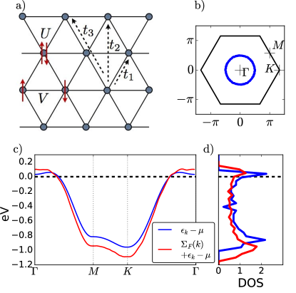
Figure 1: a) The triangular lattice, with the hopping and interaction parameters. The hopping is parametrized up to the third nearest neighbour and the interaction is parametrized up to the nearest neighbour. b) The 1st Brillouin zone of the triangular lattice, with high-symmetry points. Blue: the non-interacting Fermi surface. c) The bare dispersion $\varepsilon(\mathbf{k}-\mu)$, together with the dispersion modified by the Fock self-energy. The chemical potential lies close to the band edge, such that the filling per spin is $\braket{n_{\sigma}}=0.83$ (1.67 electrons per site). d) Corresponding densities of states. Note the two van Hove singularities, corresponding to a flattening in the band dispersion.

The minimal model to study the interplay between local and non-local interactions, and the induced screening processes, is the extended Hubbard model, the Hamiltonian of which is given by:

$$\mathcal{H}=\sum_{i,j,\sigma}t_{ij}c_{i\sigma}^{\dagger}c_{j\sigma}+U\sum_{i}n_{i\uparrow}n_{i\downarrow}+V\sum_{\braket{i,j}}n_{i}n_{j},$$ (1)

where $c_{i\sigma}^{\dagger},c_{i\sigma}$ are electronic creation and annihilation operators, respectively, for site $i$ and spin $\sigma$; $n_{i}=n_{i\uparrow}+n_{i\downarrow}=c_{i\uparrow}^{\dagger}c_{i\uparrow}+c_{i\downarrow}^{\dagger}c_{i\downarrow}$ is the total density on site $i$. The sum $\sum_{i}$ runs over all lattice sites, while $\sum_{\braket{i,j}}$ runs over all nearest neighbour lattice bonds. The first term of Eq. (1) is the non-interacting part and accounts for the hopping of the electrons between the sites. The second and third terms are the interacting part, and account for Coulomb repulsion. The second term is an on-site Hubbard repulsion term. The third term is a nearest-neighbour (non-local) Coulomb repulsion. Hence, the extended Hubbard model is able to capture the interplay between correlations induced by local and non-local interactions.

The Hamiltonian (1) can be recast in the more compact form:

$$\mathcal{H}=\sum_{i,j,\sigma}t_{ij}c_{i\sigma}^{\dagger}c_{j\sigma}+\frac{1}{2}\sum_{i,j}v_{ij}n_{i}n_{j},$$ (2)

where we have defined the real-space interaction $v_{ij}=U\delta_{ij}+V\delta_{\braket{i,j}}$. The Fourier transform of $v_{ij}$ has the following expression:

$$v_{\mathbf{k}}=U+2V\left(\cos(k_{x})+2\cos\left(\frac{k_{x}}{2}\right)\cos\left(\frac{\sqrt{3}k_{y}}{2}\right)\right).$$ (3)

Our model is depicted in Fig. 1(a), the corresponding Brillouin zone in Fig. 1(b). The non-interacting part of the Hamiltonian, Eq. (1), is chosen such as to reproduce the band dispersion of a typical two-dimensional transition metal oxide, namely the LDA band structure of Na_2/3CoO₂, as presented by Piefke et al.Piefke et al. (2010). In the Hamiltonian, Eq. (1), the hopping parameters $t_{ij}$ are the inverse Fourier transform of $\varepsilon_{\mathbf{k}}$, represented in Fig. 1(c). More specifically, $\varepsilon_{\mathbf{k}}$ is parametrized up to the third nearest neighbour, with:

$$t_{1}=-0.134\text{ eV, }\phantom{mn}t_{2}=+0.028\text{ eV, }\phantom{mn}t_{3}=-0.024\text{ eV},$$ (4)

via the dispersion relation:

$$\begin{split}\varepsilon_{\mathbf{k}}=&2t_{1}\left(\cos(k_{x})+2\cos(k_{x}/2)\cos(k_{y}\sqrt{3}/2)\right)\\ &+2t_{2}\left(\cos(\sqrt{3}k_{y})+2\cos(3k_{x}/2)\cos(k_{y}\sqrt{3}/2)\right)\\ &+2t_{3}\left(\cos(2k_{x})+2\cos(k_{x})\cos(\sqrt{3}k_{y})\right).\end{split}$$ (5)

The hopping parameters $t_{ij}$ are in the range of 100 meV, but due to the high connectivity of the triangular lattice, the non-interacting bandwidth is approximately 1.1 eV, as can be seen in the non-interacting density of states in Fig. 1(d).

Since we aim at probing the system in the high-doping regime, we set the band filling to $\braket{n_{\sigma}}=0.83$ (corresponding to an average of 1.67 electrons per atomic site). Note that this particular filling corresponds to a large non-interacting density of states at the Fermi level. The non-interacting Fermi surface is composed of a single hole pocket centered around the $\Gamma$ point.

In our study, we will vary the onsite interaction $U$ up to 4 eV and the intersite $V$ up to 0.7 eV. In the following, all energies are given in electron-volts.

II Methods

II.1 Computational schemes

The extended Hubbard Hamiltonian, Eq. (1), is a many-body Hamiltonian; physical observables can therefore only be computed by using approximations. Here, we take a strongly correlated perspective to study the interplay between local and non-local interactions, and quantum hopping. Also, we want to access single-particle properties (as given by the one-body Green’s function and relevant for photoemission experiments) and screening (as encoded in the two-body Green’s function) on the same footing. Whereas dynamical mean-field theory (DMFT) can describe the interplay between local interaction and quantum hopping, extended DMFT is able to account for non-local interactions. In the following, we review these two methods. Then we describe how to optionally include a non-local Fock diagram.

II.1.1 Reminder on the (extended) dynamical mean-field approximation

Dynamical mean-field theories aim at computing observables on the lattice through a self-consistent loop, using an Anderson impurity model as a reference system. In the following, the subscript “imp” refers to impurity quantities, while the subscript “loc” refers to the local (i.e., site-diagonal) part of lattice quantities.

Single-site dynamical mean-field theory (DMFT) assumes that the local part of the lattice Green’s function can be generated as the solution of a local impurity problem embedded into a bath. The latter is determined self-consistently, using the impurity self-energy as an approximation to the full self-energy of the lattice problem in the calculation of the local lattice Green’s function.

Via this construction, local quantum fluctuations on the single-particle level are treated to all orders in perturbation theory, resulting in a frequency-dependent self-energy Kotliar and Vollhardt (2004). The self-energy $\Sigma_{\mathrm{imp}}$ and the impurity Green’s function, $G_{\mathrm{imp}}$, are computed by solving a self-consistently determined Anderson impurity model:

$$\begin{split}S^{\text{DMFT}}_{\text{imp}}[c^{*},c]=&-\sum_{\sigma}\iint_{0}^{\beta}\mathrm{d}\tau\mathrm{d}\tau^{\prime}c^{*}_{\sigma}(\tau)\mathcal{G}_{0}^{-1}(\tau-\tau^{\prime})c_{\sigma}(\tau^{\prime})\\ &+\frac{U}{2}\int_{0}^{\beta}\mathrm{d}\tau n(\tau)n(\tau).\end{split}$$ (6)

The path-integral action Eq. (6) is expressed in imaginary time $\tau$ and $\beta$ is the inverse temperature. The Grassmann variables $c^{*},c$ correspond to the fermionic operators $c^{\dagger},c$ respectively. We denote $n=\sum_{\sigma=\uparrow,\downarrow}c_{\sigma}^{*}c_{\sigma}$.

The dynamical mean field $\mathcal{G}_{0}$ is a self-consistent quantity. The self-consistency condition ensures that the local part of the lattice Green’s function is given by the impurity Green’s function, $G_{\mathrm{loc}}=G_{\mathrm{imp}}$, calculated under the approximation that the self-energy of the lattice is local and given by the impurity. The DMFT self-consistency loop is summarized on the left handside of Fig. 2.

DMFT becomes exact in the limit of infinite coordination Metzner and Vollhardt (1989a, b), where non-local quantum fluctuations average out, resulting in a purely local lattice self-energy. For a finite dimensional lattice, DMFT yields an approximation that can be interpreted in two ways: the straightforward interpretation consists in saying that the lattice self-energy is approximated by a purely local quantity generated from the impurity problem. This view can be expressed by saying that the lattice self-energy has the following functional dependence:

$$\Sigma_{ij}=\delta_{ij}\,\Sigma_{\mathrm{imp}}[G_{\mathrm{imp}},U]$$ (7)

where $i,j$ denote site indices. $i\omega$ (and later $i\nu$) denote fermionic (resp. bosonic) Matsubara frequencies. A more subtle interpretation offers itself when restricting the observables of interest to the local part of the lattice Green’s function: DMFT assumes that this part can be generated from a local impurity model, using the self-consistently calculated bath. In the latter case, no explicit assumption on the lattice self-energy is made, and the logic of the theory becomes comparable to the DFT construction, where a Kohn-Sham potential is calculated for the mere purpose of generating the physical density, but without any assumption on its relevance for the physical system. From this perspective, the impurity model is the equivalent of the Kohn-Sham system, and the construction of the local self-energy from the impurity problem with the self-consistent bath the analogue of the local density approximation to Kohn-Sham theory.

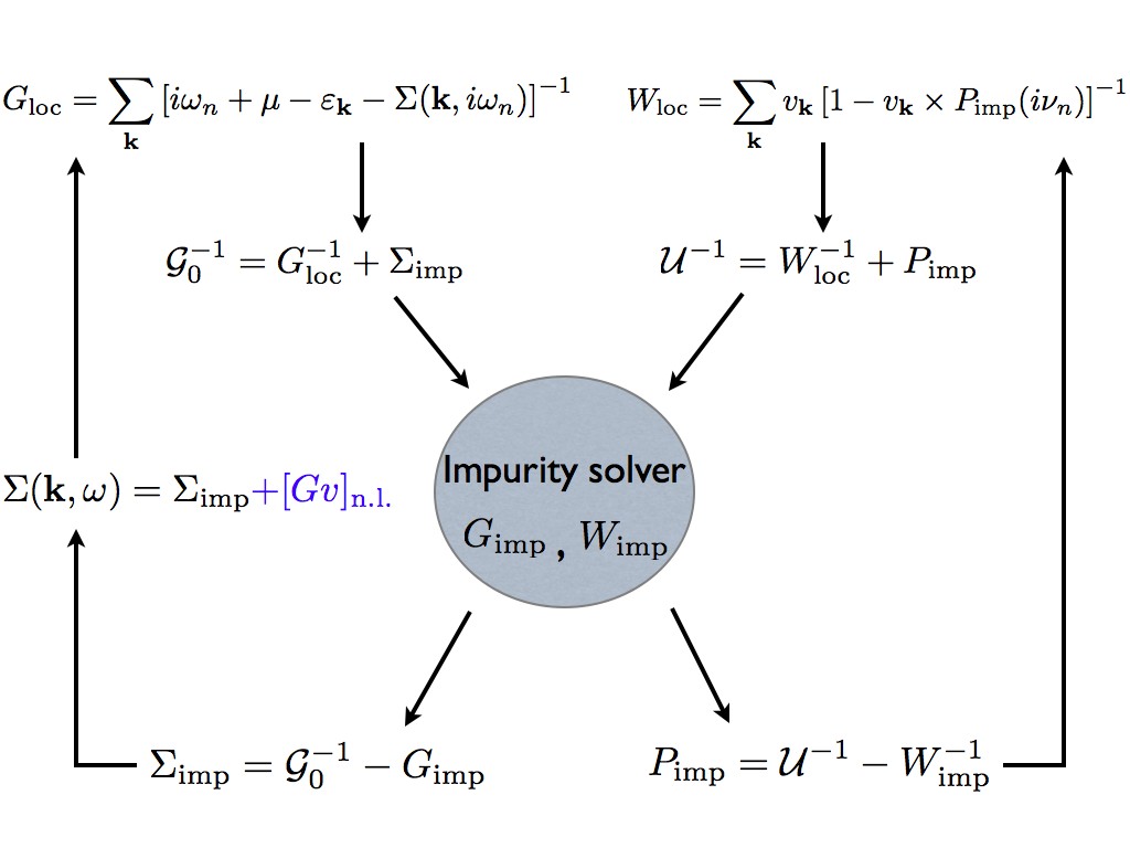
Figure 2: The (Fock +) extended dynamical mean-field self-consistent loop. A non-local Fock term (blue) is optionally included in the self-energy, leading to the Fock+EDMFT scheme. Without the Fock term, the left part of the scheme reduces to the DMFT self-consistency loop.

DMFT is designed to compute one-particle observables. Thus, just as Kohn-Sham theory yields the density but no other observables, DMFT may not properly capture two-particle observables. Even more importantly, in the present context, it disregards non-local interactions, and makes no attempt of addressing screening processes induced by the latter.

In EDMFT, a bosonic propagator, $W$, is introduced, coupling to charge fluctuations introduced by a non-local interaction, $V$. Thus, EDMFT is designed to compute both one-particle and two-particle observables. Here, the two-particle observables are computed only in the charge channel. The bosonic propagator $W$ can be identified with the screened Coulomb interaction. It has a self-energy, $P$, the polarization (or irreducible polarisability).

Again, the self-energy, impurity Green’s function, the polarization $P_{\mathrm{imp}}$ and the screened interaction of the impurity $W_{\mathrm{imp}}$, are computed self-consistently by solving a local model, now featuring an effective bare local interaction, $\mathcal{U}(i\nu_{n})$:

$$\begin{split}S^{\text{EDMFT}}_{\text{imp}}[c^{*},c]=&-\sum_{\sigma}\iint_{0}^{\beta}\mathrm{d}\tau\mathrm{d}\tau^{\prime}c^{*}_{\sigma}(\tau)\mathcal{G}_{0}^{-1}(\tau-\tau^{\prime})c_{\sigma}(\tau^{\prime})\\ &+\frac{1}{2}\iint_{0}^{\beta}\mathrm{d}\tau\mathrm{d}\tau^{\prime}\mathcal{U}(\tau-\tau^{\prime})n(\tau)n(\tau^{\prime}).\end{split}$$ (8)

EDMFT treats non-local interactions, $v_{ij}$, by transforming them into a frequency-dependent local interaction, $\mathcal{U}(i\nu_{n})$ Gatti et al. (2007). $\mathcal{U}$ and $\mathcal{G}_{0}$ are both determined self-consistently. The self-consistency condition is now that both local quantities, $G_{\mathrm{loc}}$ and $W_{\mathrm{loc}}$, are given by the impurity: $G_{\mathrm{loc}}=G_{\mathrm{imp}}$ and $W_{\mathrm{loc}}=W_{\mathrm{imp}}$, under the approximation that the self-energy and the polarization are local and given by the impurity. The EDMFT self-consistency loop is summarized in Fig. 2.

As DMFT, EDMFT is a non-perturbative scheme, particularly well suited for systems with strong interactions, dominated by local self-energy and polarization processes. Similarly to the first interpretation of DMFT (see above), single-site EDMFT can be interpreted as an approximation that assumes both the fermionic self-energy $\Sigma$ and the polarization $P$ to be local and to be given by the sum of all local diagrams. This can be expressed by the functional dependence of the EDMFT self-energy and polarization:

$$\Sigma_{ij}(i\omega)=\delta_{ij}\,\Sigma_{\mathrm{imp}}[G_{\mathrm{imp}},W_{\mathrm{imp}}](i\omega),$$ (9a)

$$P_{ij}(i\omega)=\delta_{ij}\,P_{\mathrm{imp}}[G_{\mathrm{imp}},W_{\mathrm{imp}}](i\omega).$$ (9b)

When adopting this interpretation, not only local quantities (local Green’s function and local screened interaction) become accessible to calculations but also their full lattice counterparts can be deduced from the self-consistent self-enery and polarization.

Analogously to the discussion above, one can also define a “purist’s point of view”, where only the arguments of the EDMFT approximation to Almbladh’s $\Psi[G,W]$ functional Almbladh et al. (1999), namely the local Green’s function $G_{loc}$ and the local screened Coulomb interaction $W_{loc}$, are accessible quantities, and the local self-energy $\Sigma_{loc}$ and the local polarization $P_{loc}$ are considered as fictitious functions at the same level as the Kohn-Sham potential of density functional theory. Indeed, mathematically speaking, $\Sigma_{loc}$ and $P_{loc}$ enter the theory as Lagrange multipliers imposing physical values to $G_{loc}$ and $W_{loc}$. This standpoint highlights that, strictly speaking, deducing lattice Green’s functions or lattice susceptibilities goes beyond the EDMFT framework in the same way as interpreting Kohn-Sham band structures of DFT as excitations of a system lies outside the initial purpose of DFT.

Here, we will adopt a hybrid point of view: we will indeed calculate and analyze the lattice screened interaction and related quantities, though we will not make use of lattice Green’s functions. One may consider this approach as analogous to the current practice of analyzing Kohn-Sham band structures from DFT, or momentum-resolved spectral functions from DMFT (even though it is likely that quite generically the approximation of a local polarization is more severe than the one of a local self-energy). Especially in two dimensions, where nonlocal effects beyond mean field are expected to be quite large, the local approximation to the polarization function is certainly a strong assumption. EDMFT should therefore be regarded as an exploratory tool to get qualitative insights into the charge dynamics.

For completeness, let us mention that several extensions of EDMFT to describe nonlocal self-energy and polarization processes have been devised in recent years. The $GW$+EDMFT method Biermann et al. (2003); Sun and Kotliar (2004) supplements the local self-energy and polarization diagrams with the nonlocal contributions from the $GW$ self-energy and $GG$ bubble polarization. The former contains non-local screening processes and the latter captures, in particular, nesting features of the Fermi surface. The first self-consistent implementation of the $GW$+EDMFT method has been developed in the context of square and cubic lattices at half-filling Ayral et al. (2012, 2013). Recently, the nonlocal Fock correction to the self-energy (which is also contained in GW) has been shown to yield important corrections to the phase boundary to the charge-ordered phase for large values of the local interaction Ayral et al. (2017) (which motivates the approximation we introduce in the next subsection). Furthermore, thanks to its relative simplicity, the $GW$+EDMFT method has also been applied to a number of realistic materials, ranging from systems of adatoms on semiconducting surfaces Hansmann et al. (2013, 2016) to the prototypical example of correlated materials, $\mathrm{SrVO}_{3}$ Tomczak et al. (2012, 2014); Boehnke et al. (2016).

Further extensions like the dual boson method Rubtsov et al. (2012); van Loon et al. (2014); Stepanov et al. (2016a) have been proposed to remedy some of the shortcomings of EDMFT and $GW$+EDMFT, like a poor description of collective modes Hafermann et al. (2014) and inconsistencies between different ways of computing susceptibilities van Loon et al. (2015). These approaches, in their full-fledged form, require the (costly) computation of impurity vertices with three and four external legs, making them hard to apply in realistic settings or to map out entire phase diagrams with state-of-the-art algorithms. Therefore, simplified versions of these methods are emerging Stepanov et al. (2016b) which do not require the computation of these vertices. Interestingly, they yield phase diagrams very similar to those obtained in $GW$+EDMFT Ayral et al. (2017), and qualitatively at least, in EDMFT.

II.1.2 Combining extended dynamical mean-field theory with a non-local Fock diagram

On top of the purely local self-energy diagrams treated by DMFT or EDMFT, we explore the addition of a non-local Fock term. Indeed, let us have a look at the first perturbative self-energy diagrams of the extended Hubbard Hamiltonian, Eq. (1). The Hartree and Fock self-energies are, respectively:

$$\Sigma^{H}_{ij,\sigma}(i\omega)=\Sigma^{H}_{ii,\sigma}\delta_{ij}=\left(Un_{i,\bar{\sigma}}+V\sum_{\braket{i,l}}n_{l}\right)\delta_{ij},$$ (10)

$$\Sigma^{F}_{ij,\sigma}(i\omega)=-\delta_{\braket{ij}}VG_{ij,\sigma}(\tau=0^{+}),$$ (11)

The Hartree terms are local and static, so they can be absorbed in a redefinition of the chemical potential, $\tilde{\mu}=\mu-\frac{U}{2}\sum_{\sigma}n_{i\sigma}-V\sum_{\braket{i,l},\sigma}n_{l\sigma}$, provided that the charge density is homogeneous. The Fock term, however, is static but non-local and, by definition, is not included in the DMFT or EDMFT schemes.

The Fock term contributes a static, non-local, real part to the self-energy. Thus, at self-consistency, it can be viewed as a modification of the bare dispersion, $\varepsilon_{\mathbf{k}}$. In practice, it leads to a widening of the non-interacting band, Fig. 1. To this renormalized effective non-interacting band, it is possible to ascribe a density of states. At the Fermi level, the renormalized density of states is lower than the bare density of states.

Hence, the usual EDMFT scheme does not include all the first-order diagrams in $V$. In the Fock+EDMFT scheme, we make sure that at least the Hartree-Fock diagrams are present, on top of EDMFT. Fock+EDMFT can be viewed as a poor man’s $GW$+EDMFT. Concerning the description of screening it goes beyond Hartree-Fock, because some screening is included via local polarization processes. We also note the relation to the recent “Screened Exchange Dynamical Mean Field Theory” (“SEx+DMFT”) van Roekeghem et al. (2014); van Roekeghem and Biermann (2014); van Roekeghem et al. (2016), an approximation to $GW$+DMFT, where the non-local $GW$ self-energy is replaced by a screened exchange term.

II.2 Implementation details

The algorithm of Fig. 2 is implemented using the TRIQS toolbox Parcollet et al. (2015). The impurity problem (Eq. (8)) is solved with a continuous-time quantum Monte-Carlo solver (CTQMC Rubtsov et al. (2012)), using a hybridization expansion Werner et al. (2006) in the segment picture, with frequency-dependent interactions $\mathcal{U}(i\nu_{n})$ Werner et al. (2009).

The impurity solver computes the fermionic self-energy, $\Sigma_{\mathrm{imp}}(i\omega)$ using improved estimatorsHafermann et al. (2012) and the polarization from the charge susceptibility:

$$\chi_{\mathrm{imp}}(\tau)=\braket{\mathcal{T}_{\tau}n(\tau)n(0)}-\braket{n}^{2}$$ (12)

using the expression:

$$P_{\mathrm{imp}}(i\nu_{n})=-\frac{\chi_{\mathrm{imp}}(i\nu_{n})}{1-\mathcal{U}(i\nu_{n})\chi_{\mathrm{imp}}(i\nu_{n})}.$$ (13)

All calculations are made assuming a paramagnetic solution, i.e. by symmetrizing the up- and down-spin components in the self-energy. The calculations use a single-site impurity and assume a homogeneous solution. The first Brillouin zone is discretized with $32\times 32$ k-points. In the calculations including the Fock term, a mixing of 50% on the local self-energy is used to stabilize the iterative cycle and finally achieve convergence. Analytic continuations are carried out using using the Maximum Entropy algorithm in Bryan’s implementationBryan (1990).

III Phase diagram

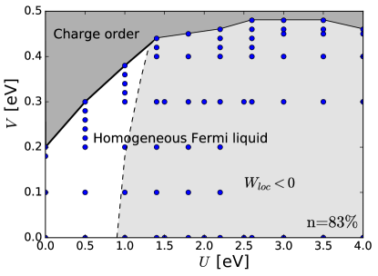
Figure 3: The EDMFT phase diagram of the extended Hubbard model on a triangular lattice, at filling per spin $\braket{n_{\sigma}}=0.83$ and inverse temperature $\beta=100$ for the paramagnetic case. It displays a second-order phase transition, between a homogeneous Fermi-liquid phase (at low $V$) and a charge-ordered region (at high $V$, dark grey). The homogeneous Fermi-liquid phase is divided into a positive static screening region (at low $U$, white) and a negative static screening region (at high $U$, light grey). The dots indicate the parameters used in the various runs that we performed.

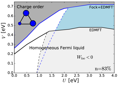
Figure 4: Comparison between EDMFT and Fock+EDMFT phase diagrams of the extended Hubbard model on a triangular lattice, at filling per spin $\braket{n_{\sigma}}=0.83$ and inverse temperature $\beta=100$ (homogeneous paramagnetic calculations). It displays a phase transition, between a homogeneous Fermi-liquid phase (at low $V$) and a charge-ordered phase (at high $V$, dark grey). The homogeneous Fermi-liquid phase is divided into a positive static screening region (at low $U$, white) and a negative static screening region (at high $U$, light grey/blue). The inset shows the charge-ordering pattern, where two atoms retain two electrons each and one atom retains one electron.

In this section, we present the phase diagram (see Figs. 3 and 4) of the triangular lattice at filling per spin $\braket{n_{\sigma}}=0.83$ and inverse temperature $\beta=100$ (corresponding to a temperature of 116 K), computed within (Fock +) EDMFT, in the homogeneous paramagnetic case. This phase diagram displays two regions: at low $V$, a region where a homogeneous metallic solution is found and a region where such a solution is no longer stable, giving way to one or possibly more charge-ordered phases.

III.1 Homogeneous metallic region

At small intersite interaction $V$, the system is in a homogeneous Fermi-liquid phase. The metallic character extends to high Hubbard interactions $U$, because the system is strongly doped (the single band being filled at 83%).

The Fermi-liquid phase is divided into two sub-regions, depending on the value of the computed local static screening, $W_{\mathrm{loc}}(\omega=0)$ (more details are provided in Sec. V). For low enough values of $U$, the local static screening is found to be positive: $W_{\mathrm{loc}}(\omega=0)>0$. However, for higher values of $U$, the local static screening is found to be negative: $W_{\mathrm{loc}}(\omega=0)<0$ (see shaded region in Fig. 4).

III.2 Transition line

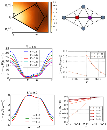
Figure 5: a) The static value of $1-v_{\mathbf{q}}P_{\mathrm{imp}}(\omega=0)$ in the irreducible Brillouin zone of the triangular lattice, for $U=2.2$ eV, $V=0.46$ eV, $\beta=100$ eV^-1, computed within EDMFT. The high-symmetry points $\Gamma$, $K$ and $M$ are represented. The $\mathbf{q}$-point where $1-v_{\mathbf{q}}P_{\mathrm{imp}}(\omega=0)$ goes to 0 is the point where the divergence of the static susceptibility, $\chi(\mathbf{q},\omega=0)$, sets in. b) and d) The static value of the dielectric function $1-v_{\mathbf{q}}P_{\text{imp}}$ on a $\mathbf{q}$-point path. Note the sign change of the dielectric function with respect to $U$. The positive sign occurs on the low-$U$ region of the phase diagram (see white region in Fig. 3); the negative sign occurs in the high-$U$ region (see light-grey region in Fig. 3). c) and e) The value of the static dielectric function for the ordering vector $\mathbf{q}_{\text{CO}}=K$, for various values of $U$.

The Fermi-liquid phase is separated from a charge-ordered region, for high values of the intersite interaction $V$. In this region of parameter space, calculations within homogeneous (Fock +) EDMFT could not be converged. The separation line in Fig. 4 marks the last converged point. More specifically, the separation line between the two phases can be monitored by the divergence of the static susceptibility $\chi(\mathbf{q}_{\text{CO}},\omega=0)$, at some ordering vector $\mathbf{q}_{\text{CO}}$. The lattice susceptibility is linked to the bosonic propagator on the lattice: $W(\mathbf{q},i\omega)=v_{\mathbf{q}}-v_{\mathbf{q}}\chi(\mathbf{q},i\omega)W(\mathbf{q},i\omega)$. The EDMFT lattice susceptibility is given by:

$$\chi(\mathbf{q},i\omega)=-\frac{P_{\mathrm{imp}}(i\omega)}{1-v_{\mathbf{q}}P_{\mathrm{imp}}(i\omega)},$$ (14)

where the $\mathbf{q}$-dependence on the right-hand side is only present in the Fourier-transform of the interaction, $v_{\mathbf{q}}$, as given by Eq. (3). The divergence of the static susceptibility $\chi(\mathbf{q},\omega=0)$ always occurs at $v_{q_{CO}}=1/P_{\mathrm{imp}}(0)$ which leads for our model to an ordering vector $\mathbf{q}_{\text{CO}}=K$ (see Fig. 1 and Fig. 5).

The divergence condition $1-v_{\mathbf{q}}P_{\mathrm{imp}}(i\omega)=0$ for the susceptibility (Eq. (14)) is equivalent to the fact that the static dielectric function goes to 0, suggesting an instability to occur. The static dielectric function is monitored in Fig. 5 in the vicinity of the charge-ordering transition.

On top of going to zero at the phase transition, the static dielectric function changes sign depending on the region of the phase diagram (see shaded region in Fig. 4, denoting negative static local screening).

III.3 Charge-ordered region

The ordered phase(s), at larger $V$, cannot be accessed via homogeneous single-site EDMFT, because of the symmetry breaking. At the specific commensurate doping $0.833=\frac{1}{2}+\frac{1}{3}$, the filling is suggestive of a $\sqrt{3}\times\sqrt{3}$ ordering, with 3 atoms per supercell: 2 atoms are completely filled and one atom retains one electron (see Fig. 4).

III.4 Comparison of the EDMFT and Fock+EDMFT phase diagrams

Upon addition of the Fock term, the charge-order transition line is pushed up in $V$. This is linked to a decrease in $\chi(\omega=0)$, connected to a decrease in the renormalized density of states at the Fermi level, $N(\epsilon_{F})$, as will be explained in section V.

In the remaining part of this study, we analyze the homogeneous Fermi-liquid phase. We give a description of correlation effects by analyzing single-particle observables in section IV and two-particle observables in section V.

IV One-particle observables

In this section, we describe the single-particle observables within EDMFT, in the Fermi-liquid phase. We argue that they are typical of a (moderately) correlated system, as they feature a lower Hubbard band.

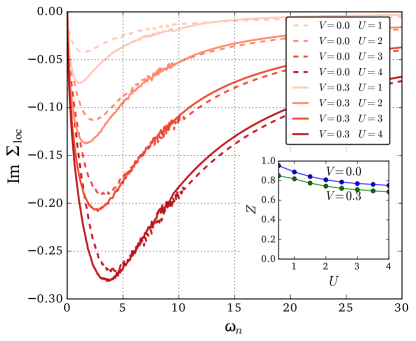
Figure 6: The imaginary part of the impurity self-energy on the Matsubara axis, Im $\Sigma_{\text{imp}}(i\omega_{n})$ within EDMFT, for various values of $U$ and $V$, and the corresponding quasi-particle renormalization factor, $Z$. The numerical values are typically those of a moderately correlated system. Correlations increase when either $U$, the on-site interaction, or $V$, the nearest-neighbour interaction, increases.

The self-energies on the Matsubara axis are depicted in Fig. 6, for various values of $U$ and $V$. The self-energies are metallic and Fermi-liquid-like (since the imaginary part of the self-energy goes linearly to zero at $\omega=0$), even for high values of the Hubbard interaction $U$. A Mott metal-insulator transition is thus prevented by the strong doping, as expected. Correlations increase when either $U$ or $V$ increases, as can be seen from the quasi-particle renormalization factors in Fig. 6. The quasi-particle renormalization factor $Z$ is defined as:

$$Z=\frac{1}{1-\left.\frac{\partial\Sigma(i\omega)}{\partial(i\omega)}\right|_{\omega=0}}.$$ (15)

The values of the renormalization factor are typical of (weakly) correlated regimes, even at strong local interaction $U$. It is worth noting that the correlations increase when the nearest-neighbour interaction $V$ increases. This trend is opposite to what was observed for the half-filled extended Hubbard model on a square lattice Ayral et al. (2013), where correlations decrease when $V$ increases. In Ref. Ayral et al., 2013, it was argued that the intersite interaction $V$ effectively reduces the on-site interaction $U$ to the screened value $U_{\text{eff}}=\mathcal{U}(i\nu_{n}=0)$. In our case, the effect of $V$ is to enhance correlations, probably because of the energetic cost associated to hopping processes taking place on sites that are nearest neighbours to occupied sites.

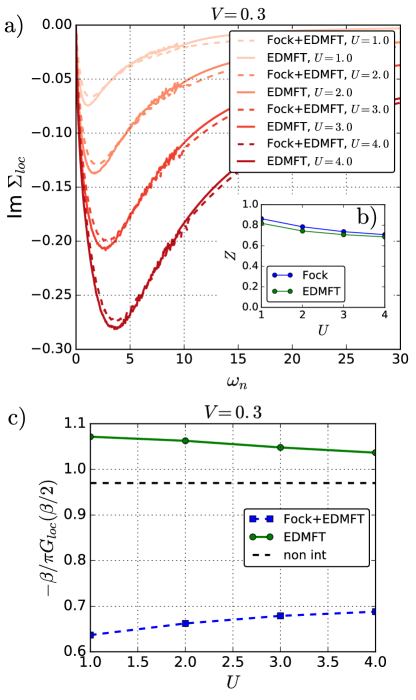
Figure 7: Comparison between EDMFT and Fock+EDMFT for various one-particle quantities. a) Imaginary part of the impurity self-energy on the Matsubara axis. b) Corresponding renormalization factors. c) Density of states at the Fermi level, computed as $N(\varepsilon_{F})\approx-\frac{\beta}{\pi}G_{\text{loc}}(\frac{\beta}{2})$. One of the effects of the Fock term is to reduce the interacting density of states at the Fermi level, as compared to both EDMFT and the non-interacting system.

Fig. 7 shows a comparison between EDMFT and Fock+EDMFT for some single-particle quantities. Concerning self-energies and renormalization factors, adding a Fock non-local term does not change the result significantly. The densities of states at the Fermi level, estimated as $N(\epsilon_{F})\approx-\beta/\pi G_{\text{loc}}(\beta/2)$, are, however, different. This is an effect of the reduction of the effective density of states when going from EDMFT to Fock+EDMFT (see Fig. 1 and the widening of the effective non-interacting band).

In Fig. 8, we display the self-energies on the real frequency axis, as obtained from the Matsubara frequency data via an analytic continuation using the maximum-entropy algorithm. The imaginary part is negative, as required by causality, and its absolute value represents (up to a factor of $\pi$) the inverse lifetime of excitations. It takes on small values around the Fermi level (the origin of the frequency axis), corresponding to the Fermi liquid nature of the metallic phase investigated here. Its most prominent property is the pronounced asymmetry of filled and empty parts of the spectrum, corresponding to the large doping, inducing much shorter lifetimes for hole excitations than for electrons. Interesting to note is also the frequency scale on which the self-energy varies, namely between -10 and 2 eV, corresponding to the energy scale of the spectral function (see below).

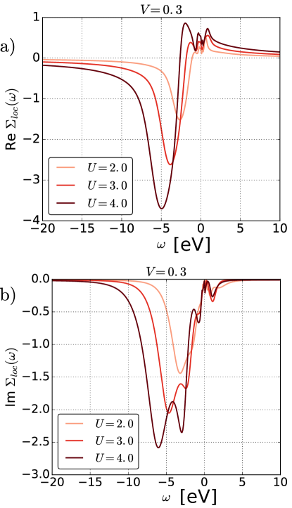
Figure 8: Self-energy as a function of real frequency, obtained from analytic continuation of the imaginary frequency data: (a) real and (b) imaginary parts of the self-energy for $V$=0.3 and varying $U$.

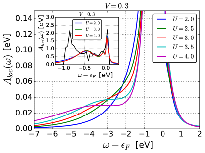
Figure 9: Local spectral functions from EDMFT, calculated as $A_{\text{loc}}(\omega)=\sum_{\mathbf{k}}A(\mathbf{k},\omega)$. The main and inset panels display the same functions on a different scale. Black: the non-interacting density of states, as in Fig. 1. Inset: The renormalization of the quasi-particle is visible on the total quasi-particle width. Main: A broad lower Hubbard band is visible, at energies between -4 eV and -3 eV. There is no visible upper Hubbard satellite.

Fig. 9 shows local spectral functions, in EDMFT, defined as $A_{\text{loc}}(\omega)=-\frac{1}{\pi}\text{Im}G_{\text{loc}}(\omega)$ and obtained via analytic continuations to the real-frequency axis using the maximum-entropy algorithm. In the inset, the spectra are represented on top of the non-interacting density of states. In the interacting spectrum, two quasi-particle structures – one narrow and one broad – are visible, corresponding to the two van Hove singularities in the DOS. As can be expected from the values of $Z$ and since the self-energy is local, the broader quasi-particle feature is renormalized (resulting in a shift of its maximum towards the Fermi level) as compared to the non-interacting case, and the bandwidth is reduced. On the main figure, the same spectra are zoomed in, to highlight a lower Hubbard band for high values of $U$. There is no upper Hubbard band. We interpret this asymmetry in the spectral function as a signature of the strong doping. Indeed, if one imagines a finite but large system, completely filled except for one hole, then the photoemission spectrum is going to be very asymmetric. On the one hand, hole-removal (or, equivalently, electron-addition) energies exactly correspond to the non-interacting ones, hence the absence of an upper Hubbard band. On the other hand, hole-addition (or, equivalently, electron-removal) energies have to take into account the interaction between two holes, hence creating a lower Hubbard band. Note that one can distinguish this Hubbard band from a satellite that would originate from electron-hole excitations contained in the frequency-dependent screening as it is the case e.g. in GW, since the latter displays structure below 1 eV (see Fig.12), whereas the hole-hole interaction is of the order of $U$, consistent with the observed distance from the quasi-particle feature (Fig.9).

V Two-particle observables

In this section, we describe our results for two-particle quantities corresponding to neutral charge excitations, in the homogeneous Fermi-liquid phase of the phase diagram Fig. 4. We argue that the two-particle observables are typical of a dilute system, with few charge carriers. They appear uncorrelated, as they do not retain traces of the Hubbard satellite present in the single-particle quantities. We first describe the impurity susceptibility, screened and effective bare interactions, and then turn to a more detailed analysis of the particularities of the high-doping regime.

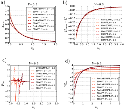
Figure 10: Comparison between EDMFT and Fock+EDMFT for various two-particle quantities on the Matsubara axis. a) The impurity susceptibility, $\chi_{\text{imp}}(i\nu_{n})$. For each method (EDMFT or Fock+EDMFT) the susceptibility is almost constant as a function of $U$. The susceptibilities within Fock+EDMFT are smaller than the susceptibilities within EDMFT. b) The dynamical interaction minus the local interaction, $\mathcal{U}(i\nu_{n})-U$. c) The impurity polarization, $P_{\text{imp}}(i\nu_{n})$. For the analyzed values of $U$ and $V$, the polarization displays a pole on the Matsubara axis. d) The local part of the screened interaction, $W_{\text{loc}}(i\nu_{n})$. The $\nu_{n}=0$ value can become negative for large enough values of $U$.

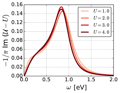
Figure 11: Effective dynamical interaction on the real frequency axis, as calculated from an analytic continuation using the Padé scheme.

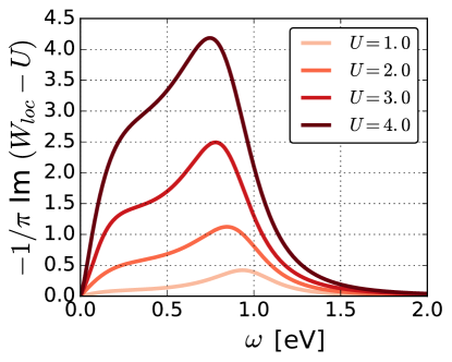
Figure 12: Local part of the screened interaction, on the real frequency axis, as calculated from an analytic continuation using the Padé scheme.

V.1 The impurity susceptibility

The local charge susceptibility $\chi_{\mathrm{imp}}(\tau)=\braket{\mathcal{T}n(\tau)n(0)}-\braket{n}^{2}$ has been computed from the Anderson impurity model in imaginary time. It is thus a single-site dynamical quantity, which is positive on the imaginary time and Matsubara frequency axes. Its Matsubara axis representation is plotted in Fig. 10(a) for several values of $U$, both within pure EDMFT and Fock+EDMFT. As a bosonic quantity, it decays for large frequencies as $\frac{1}{\nu^{2}}$. System-specific information is therefore rather contained in the low-frequency behavior. The most striking features of the plot are (i) the weak dependence on $U$, indicating that the impurity charge susceptibility is only weakly renormalized by correlations and (ii) the marked difference between the EDMFT and Fock+EDMFT results. We will analyze both of these points in detail below.

V.2 Effective local interaction

The frequency-dependent interaction, $\mathcal{U}(i\nu_{n})$, is represented in Fig. 10(b). The real-frequency representation of its imaginary part (obtained by analytic continuation using Padé approximants) is plotted in Fig. 11. This interaction, a partially screened interaction, is an auxiliary quantity of the EDMFT scheme. It effectively mimics the effect of the non-local interaction $v_{\mathbf{k}}$ onto the local interaction, by introducing a frequency-dependence. The imaginary part can – up to a factor $-\pi$ – be understood as the density of screening modes thus generated. The Matsubara axis plot Fig. 10(b) gives the difference between $\mathcal{U}(i\nu_{n})$ and the bare interaction parameter $U$ of the model. Since at high enough frequencies screening is no longer effective, $\mathcal{U}(i\nu_{n})$ goes to $U$ in this limit, and the difference $\mathcal{U}(i\nu_{n})-U$ vanishes. At zero-frequency, $\mathcal{U}(i\nu_{n}=0)=U_{\text{eff}}<U$ goes to a screened static value. At low frequencies, $\tilde{\mathcal{U}}(i\nu_{n})=\mathcal{U}(i\nu_{n})-U$ is a measure of the screening induced by the non-local interactions. In general, the efficiency of screening depends on the charge-charge correlations, which can be strongly influenced also by the local part of the bare interaction, the Hubbard $U$. Here, we find however that this partial screening depends only weakly on the local $U$: The curves in both, Fig. 10(b) and Fig. 11, show a quite negligible $U$-dependence: To a good approximation, $\tilde{\mathcal{U}}=\tilde{\mathcal{U}}[V,\chi_{0}]$, i.e. it depends only on $V$ and on the band structure, but not on the local interaction $U$. Below, we will argue that this finding is a consequence of the weak $U$-dependence of the impurity charge susceptibility found above.

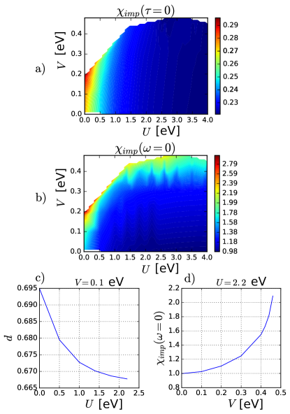
Figure 13: Analysis of the impurity susceptibility, $\chi_{\text{imp}}$ in EDMFT. a) Colour plot of $\chi_{\text{imp}}(\tau=0)$ over the whole phase diagram. $\chi_{\text{imp}}(\tau=0)$ is directly connected to the double-occupancy, $d$. b) Colourplot of $\chi_{\text{imp}}(\omega=0)$ over the whole phase diagram. A divergence in $\chi_{\text{imp}}(\omega=0)$ signals a second-order instability. c) Double-occupancy $d$ as a function of $U$ for constant $V$. d) $\chi_{\text{imp}}(\omega=0)$ as a function of $V$ for constant $U$.

V.3 Screened Coulomb interaction and polarization

Fig. 10(d) shows the fully screened Coulomb interaction on the Matsubara axis, Fig. 12 its imaginary part on the real axis. The overall shape of these quantities is similar to that of the effective interaction $\mathcal{U}$ discussed above, but the comparison of the two quantities is instructive: $W=\frac{\mathcal{U}}{1-P_{\text{imp}}\mathcal{U}}$ results from screening the effective $\mathcal{U}$ by the local impurity polarization (see Fig. 10(c)): this additional screening leads to an overall reduction of $W$ as compared to $\mathcal{U}$, which becomes obvious already from the different scales. As expected, the energy range where screening modes exist stays roughly the same (compare Fig. 11 and Fig. 12) but the coupling strength of these modes is much enhanced. Also, a more pronounced shoulder towards low frequencies in $W$ indicates an enhancement of low-energy modes. Such modes have also been found in the density-density response of the homogeneous electron gas at low densities and large wave vectors Takada (2016). Note that the local screening as included in EDMFT corresponds to an average over all wave vectors. Finally, the overall screening strength now does depend quite strongly on $U$ (see below).

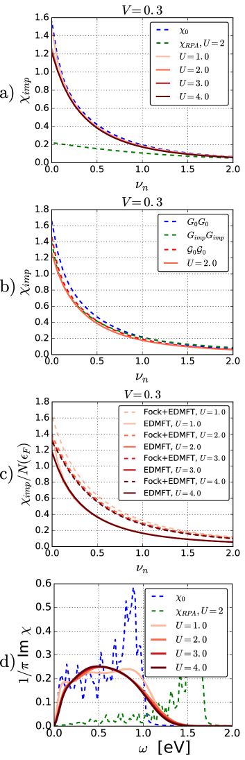
Figure 14: Analysis of the impurity susceptibility, $\chi_{\text{imp}}$. a) $\chi_{\text{imp}}(i\nu_{n})$ on the Matsubara axis within EDMFT. It is close to its non-interacting counterpart, $\chi_{0}=G_{0}G_{0}$, even for large values of $U$. b) Comparison to various (local) bubble diagrams. c) Comparison between EDMFT and Fock+EDMFT susceptibilities, both renormalized by the effective interacting density of states at the Fermi level, $N(\epsilon_{F})$ (see text). d) Analytic continuation of the EDMFT susceptibility, compared to the non-interacting susceptibility $\chi_{0}=2G_{0}G_{0}$, and the random-phase approximation (RPA) susceptibility, $\chi_{\text{RPA}}$.

V.4 Analysis of the impurity susceptibility

The weak renormalization by correlations can be understood by analyzing two components of the susceptibility: the frequency-integrated value $\chi_{\text{imp}}(\tau=0)$ and the static value $\chi_{\text{imp}}(\omega=0)$, both represented in Fig. 13, spanning various parameter sets throughout the phase diagram. $\chi(\tau=0)$ (the area under the curve $\chi(i\omega)$) is linked to the double-occupancy on the impurity, $d$, via:

$$d=\frac{1}{2}\left(\chi_{\text{imp}}(\tau=0)+\braket{n_{\uparrow}+n_{\downarrow}}^{2}-\braket{n_{\uparrow}+n_{\downarrow}}\right).$$ (16)

The double-occupancy goes from a non-interacting value (0.83*0.83) at low $U$ (the equivalent of 0.25 at half-filling), to an interacting value 1*(1.667-1) at high $U$ (the equivalent of 0 at half-filling). However, due to the filling constraint, these two values are numerically close. $\chi(\omega=0)$ is also represented. It becomes maximum at the charge-ordering transition line, indicating a second-order instability.

The impurity susceptibility is thus weakly renormalized by the local interaction $U$. In fact, in EDMFT, the susceptibility is close to its non-interacting counterpart. Let us define the local non-interacting lattice susceptibility, $\chi^{0}_{ii}(\tau)=2G^{0}_{ii}(\tau)G^{0}_{ii}(\beta-\tau)$, where $G^{0}_{ii}$ is the local lattice non-interacting Green’s function. A comparison between the impurity susceptibility and the local non-interacting lattice susceptibility is presented in Fig. 14. These quantities are numerically close to each other. In Fig. 14(b) comparison is also presented with a bubble composed of interacting Green’s functions, $2G_{\text{imp}}G_{\text{imp}}$, and at the impurity level with $2\mathcal{G}_{0}\mathcal{G}_{0}$. All these quantities are numerically close.

V.5 Comparison of EDMFT and Fock+DMFT

The effect of the Fock term on the susceptibilities can be seen in Fig. 10. The Fock+EDMFT susceptibilities are significantly smaller than the EDMFT ones. Indeed, as we have seen, the non-local Fock self-energy effectively widens the non-interacting band. This means, in particular, that $N(\epsilon_{F})$ decreases, which leads to a decrease in $\chi$ (as a reminder, for a non-interacting metal, the static susceptibility goes as $N(\varepsilon_{F})$). In Fig. 14, $\chi/N(\epsilon_{F})$ is represented, for both EDMFT and Fock+EDMFT. $N(\epsilon_{F})$ is estimated from the formula $-\beta/\pi G_{\text{loc}}(\beta/2)$, as in Fig. 7. Hence, the renormalization of the susceptibility upon addition of the Fock term can be traced back to the decrease of the density of states at the Fermi level. This decrease of the impurity susceptibility implies that when the Fock term is added, the susceptibility differs more from the non-interacting one than in the case of pure EDMFT.

Finally, we show analytic continuations of the EDMFT impurity susceptibility. The spectra retain the shape expected from the non-interacting density of states. There is no sign of the Hubbard satellite, which was present in the single-particle spectra. Two aspects may contribute to this finding: first, in the framework of Hedin’s equations, satellites in two-body spectra can be rationalized as stemming from the frequency-dependence of both the self-energy and of its derivative $\delta\Sigma/\delta G$, which contains the electron-hole interaction. From the framework of calculations based on the Bethe-Salpeter equation Bechstedt et al. (1997) and from cumulant expansions of the electron-hole Green’s function Zhou et al. (2015) it is known that these two contributions have a tendency to cancel each other. Second, in a dilute system, neutral excitations (with fixed particle number) correspond to non-interacting excitations. Thus, cancellations must be particularly efficient The weak deviation of $\chi_{\text{imp}}$ from its non-interacting counterpart can thus be linked to the high doping level, and one may expect a qualitatively similar behaviour for the lattice charge dynamics.

V.6 Consequences for the lattice charge susceptibility

As discussed in the methods section, when adopting a “purist’s point of view”, EDMFT does not give access to the lattice susceptibility. Nevertheless, keeping the limitations of the local approximation in mind, one may still ask the question of how this quantity would look like when calculated under the assumption of a purely local polarization function given by the EDMFT one, see Eq. (14).

Inspired by the analysis of the impurity polarization and the effective interaction above, we make the simplifying assumption that $\chi_{\text{imp}}$ is independent of $U$ or $V$ through the whole phase diagram and that $\chi_{\text{imp}}=\chi^{0}$. As is clear from the above analyses, the qualitative behaviour of all auxiliary quantities can be well understood in terms of this simplifying assumption. Here, we analyze the implications for the (Fock +) EDMFT lattice susceptibility. Let us decompose $v_{\mathbf{k}}=U+\Delta v_{\mathbf{k}}$, such that $\Delta v_{\mathbf{k}}$ depends only on the intersite interaction $V$. Assuming that $\chi_{\text{imp}}=\chi_{0}$, the EDMFT susceptibility, Eq. (14), can be re-expressed as:

$$\chi^{\text{EDMFT}}(\mathbf{k},\omega)=\frac{\chi_{0}}{1-\tilde{\mathcal{U}}\chi_{0}+\Delta v_{\mathbf{k}}\chi_{0}}.$$ (17)

Since $\tilde{U}=\mathcal{U}-U$ is almost independent of $U$ (see Fig. 10), the same holds for the EDMFT susceptibility.

V.7 Negative screened interaction

Finally, we report a region characterized by a negative static screening. As already mentioned in section III, in the phase diagram, Fig. 3, the Fermi-liquid phase is divided into a region where the static local screening is positive, $W_{\mathrm{loc}}(\omega=0)>0$ at small $U$’s, and a region where the static local screening is negative, $W_{\mathrm{loc}}(\omega=0)<0$ at large $U$’s. The qualitative frequency-dependence of $P_{\text{imp}}$ and $W_{\text{imp}}$ is a direct consequence of the approximate equality $\chi=\chi_{0}$. Indeed, assuming that $\chi_{\mathrm{imp}}(\omega)=\chi_{0}(\omega)$, $P_{\mathrm{loc}}$ and $W_{\mathrm{loc}}$ can be re-expressed as:

$$P_{\mathrm{loc}}=-\frac{\chi_{0}}{1-\mathcal{U}\chi_{0}}$$ (18)

$$W_{\mathrm{loc}}=\sum_{\mathbf{k}}\frac{v_{\mathbf{k}}}{1-v_{\mathbf{k}}P_{\mathrm{imp}}}=(1-\mathcal{U}\chi_{0})\sum_{\mathbf{k}}\frac{v_{\mathbf{k}}}{1+v_{\mathbf{k}}\chi_{0}}.$$ (19)

Eqs. (18) and (19) show that, depending on the value of $1-\mathcal{U}\chi_{0}$, there is a possibility for both a pole in $P_{\text{loc}}$ and a sign-change in $W_{\text{loc}}$. These quantities are represented in Fig. 10. For $V=0.3$ and $U=2$, 3, 4, $P_{\text{loc}}$ displays a pole at finite frequency, while $W_{\text{loc}}$ changes sign. In particular, at zero-frequency, $W_{\text{loc}}$ takes a negative value.

The possibility that the local static screening is negative is not an artefact of the (Fock+) EDMFT approximation. It is a feature of any system where the susceptibility is large compared to the inverse interaction: $|\chi|v_{\bf k}>1$. In appendix A, we show that such a situation is easy to generate by presenting an example of a simple exactly solvable model where $W_{\mathrm{loc}}$ becomes negative. In the EDMFT context, negative screened interactions have also been observed in the context of an extended Hubbard model on the square lattice Huang et al. (2014). If – with the caveats above – one interprets the EDMFT dielectric function as the physical dielectric function of the system, we notice that a negative local static $W$ requires a set of $q$-vectors for which the inverse dielectric function $1/\epsilon(q,\omega=0)$ is negative. In the present case, due to the structure of the bare interaction, the negative values extend over the whole first Brillouin zone, including $q\rightarrow 0$, corresponding to a negative electronic compressibility of the system.

Further situations where negative static inverse dielectric functions might appear have been discussed in the literature: a prominent example is the jellium model, an electron gas with a static uniform positive compensating background Nozières and Pines (1966), in the low density regime. However, the interpretation of this effect remains subtle. Nozières Nozières and Pines (1966) argues that in the presence of a negative electronic compressibility, the system would become unstable with respect to density fluctuations of the positive background. This would suggest that in the solid, with potentially mobile ionic degrees of freedom, the relevant quantity to analyze is the total (electronic plus ionic) compressibility rather than the electronic one alone. Explicit calculations for simple metals have been performed by Kukkonen and Wilkins Kukkonen and Overhauser (1979), where inclusion of polarization effects of the ionic cores was shown to be important. Dolgov et al. Dolgov et al. (1981), on the other hand, stress that a negative dielectric function at finite $q$-vectors does not a priori contradict the requirements of system stability. These authors review a variety of different physical systems where such a situation appears. The electron gas problem was taken up in detail by Takada Takada (2016) and Takayanagi and Lipparini Takayanagi and Lipparini (1997), who have investigated the finite $q$-behavior resulting from the negative dielectric function of the dilute electron gas: in this regime, a collective mode (“ghost plasmon” or “ghost exciton”) was identified.

In the present case, we are dealing with a region of negative $\epsilon(q,\omega=0)$ extending over the whole first Brillouin zone, thus formally corresponding to the case of negative electronic compressibility. One may speculate that the present regime indeed already corresponds to a situation where the positive ionic lattice would become unstable towards lattice distortions or phase separation.

To conclude this section, we have shown that both quantities, $P_{\text{loc}}$ and $W_{\text{loc}}$, self-consistently adjust in such a way that the approximate equality $\chi_{\text{imp}}=\chi_{0}$ is preserved. This may create a pole in the impurity polarization on the Matsubara axis. Importantly, this may cause the value of the static screening to become negative and effectively attractive.

VI Summary and Conclusions

We have studied the extended Hubbard model on the triangular lattice in a regime of high doping, close to the band-insulating limit. We have briefly described the EDMFT and the Fock+EDMFT schemes. In the latter, a non-local Fock self-energy diagram supplements the purely local diagrams of EDMFT. We have computed the phase diagram as a function of local and non-local interactions. For low intersite interactions, a homogeneous metallic phase is found. For high intersite interactions, the homogeneous phase could not be stabilized, hinting at a charge-ordered, symmetry-broken phase. In the homogeneous metallic phase, a region with negative local static screening is observed. The negativity of the static screened interaction can be traced back to the high doping, the large on-site interaction and the band structure. Within the EDMFT approximation, the present situation of a local negative screened interaction goes hand in hand with a negative compressibility (see Section V.G), signaling a possible instability of the positive background. Its consequences are an interesting open question, that would however require an extension of the model in order to include ionic degrees of freedom explicitly.

We have analyzed spectral properties within (Fock +) EDMFT in the homogeneous metallic phase at the level of one- and two-particle observables, rationalizing seemingly contradicting trends. The one-body spectral function is asymmetric owing to the high doping, and features a lower Hubbard band as a result of correlations. On the two-body level, the charge susceptibility is found to be weakly renormalized by interactions. This observation, using a non-perturbative methodology, demonstrates a remarkable failure of the random-phase approximation in our particular doping regime. Indeed, the interacting susceptibility is even less renormalized by correlations than within the RPA.

VII Perspectives

Understanding the effects of non-local interactions is of course also an issue that is relevant from a materials science perspective. Charge-ordering is an ubiquitous phenomenon in (quasi-) two-dimensional materials with a triangular lattice geometry: examples include sodium and lithium cobaltates Fouassier et al. (1973); Amatucci et al. (1996), two-dimensional organics Hotta (2012); Kagawa et al. (2013) or surface systems Hansmann et al. (2013, 2016).

The non-interacting part of our model parameters was chosen to be representative of a specific system, namely Na-doped cobaltates. These two-dimensional systems display a rich phase diagram as a function of doping Foo et al. (2004); Lang et al. (2008); Schulze et al. (2008). Interestingly, many of the intriguing properties that can be assigned to correlations occur at high doping, near the band-insulating regime. In particular, in the high-doping regime, it was found that the triangular lattice disproportionates into a lattice with a four-fold larger unit cell, forming a Kagome lattice of active sites Alloul et al. (2009). A charge ordering pattern corresponding to this symmetry breaking would correspond to an ordering vector $\Gamma-M$. Considering any realistic set of parameters $U$ and $V$ for the cobaltates (typically $U\geq 2$ eV Hasan et al. (2004)), within EDMFT, the system falls either in the negative-screening or the charge-ordered region.

In the future, it would therefore be interesting to extend our study by allowing symmetry-broken solutions in real space. Indeed, a still open interesting question is the origin of the experimentally observed charge ordering in the cobaltates, including its ordering vector. The wave vector suggested by the present EDMFT calculations does not allow to understand the experimental situation.

From the methodological point of view, it could be interesting to benchmark our phase diagram against extensions of EDMFT. In particular, the contribution from non-local self-energy and polarization diagrams could be checked by comparing our results to $GW$+DMFT Biermann et al. (2003); Sun and Kotliar (2004); Ayral et al. (2012, 2013); Biermann (2014), TRILEX Ayral and Parcollet (2015, 2016); Ayral et al. ; Vučičević et al. (2017), dual boson van Loon et al. (2014) or cluster calculations Terletska et al. (2017).

Appendix: Negative screening in the Hubbard dimer

In this appendix, we further investigate the question of the appearance of a negative local screened Coulomb interaction. In particular, we show that a negative static screening is not an artefact of the EDMFT approximation, but is expected in this low-density regime.

We show in the following that it appears in the exact solution of specific many-body systems.

Let us define the Hubbard dimer at 1/4-filling via the Hamiltonian:

$$H=U\sum_{i=1,2}n_{i\uparrow}n_{i\downarrow}-t\sum_{\sigma}(c_{1\sigma}^{\dagger}c_{2\sigma}+c_{2\sigma}^{\dagger}c_{1\sigma})-\mu\sum_{i}n_{i},$$ (20)

where $\mu$ is chosen such that the many-body ground state features one electron.

The charge susceptibility can be computed exactly and does not depend on the interaction $U$ at quarter-filling. On the Matsubara axis, the local (diagonal) component is:

$$\chi_{11}(i\nu_{n}) =-\frac{1}{4}\left[\frac{1}{i\nu_{n}-2t}-\frac{1}{i\nu_{n}+2t}\right]$$

$$=\frac{t}{\nu_{n}^{2}+4t^{2}}.$$ (21)

This is a lorentzian centered around 0. The value at the Matsubara frequency $\nu_{n}=0$ is:

$$\chi_{11}(i\nu_{n}=0)=\frac{1}{4t},$$ (22)

which goes to infinity when $t\rightarrow 0$. With the formula $W_{ij}=v_{ij}-v_{ik}\chi_{kl}v_{lj}$, where $i,j,k,l$ denote site indices, we find that for $\nu_{n}=\omega=0$:

$$W_{11}(\omega=0)=W_{\text{loc}}(\omega=0)=U-\frac{U^{2}}{4t},$$ (23)

which becomes negative as soon as $U/(4t)>1$. Hence, the fact that the local part of $W$ becomes negative is not an artifact of an approximation. It happens in our exactly-solvable model.

The off-diagonal (intersite) element of the susceptibility is given by: $\chi_{12}=-\chi_{11}$ (as it should, given the requirement of charge conservation, which imposes $\chi(q=0,0)=0$). From this, the local part of the polarization can be computed:

$$P_{11}=-\frac{\chi_{11}}{1-2U\chi_{11}}.$$ (24)

In particular, when $\chi_{11}$ grows large, then $P_{11}$ develops a pole.

References

- Imada et al. (1998) M. Imada, A. Fujimori, and Y. Tokura, Rev. Mod. Phys. 70, 1039 (1998).
- Takada et al. (2003) K. Takada, H. Sakurai, E. Takayama-Muromachi, F. Izumi, R. A. Dilanian, and T. Sasaki, Nature 422, 53 (2003).
- Terasaki et al. (1997) I. Terasaki, Y. Sasago, and K. Uchinokura, Phys. Rev. B 56, R12685 (1997).
- Tocchio et al. (2014) L. F. Tocchio, C. Gros, X.-F. Zhang, and S. Eggert, Phys. Rev. Lett. 113, 246405 (2014).
- Hotta and Furukawa (2006) C. Hotta and N. Furukawa, Phys. Rev. B 74, 193107 (2006).
- Hotta and Furukawa (2007) C. Hotta and N. Furukawa, Journal of Physics: Condensed Matter 19, 145242 (2007).
- Wessel and Troyer (2005) S. Wessel and M. Troyer, Phys. Rev. Lett. 95, 127205 (2005).
- Heidarian and Damle (2005) D. Heidarian and K. Damle, Phys. Rev. Lett. 95, 127206 (2005).
- Melko et al. (2005) R. G. Melko, A. Paramekanti, A. A. Burkov, A. Vishwanath, D. N. Sheng, and L. Balents, Phys. Rev. Lett. 95, 127207 (2005).
- Zhang et al. (2011) X.-F. Zhang, R. Dillenschneider, Y. Yu, and S. Eggert, Phys. Rev. B 84, 174515 (2011).
- Cano-Cortés et al. (2011) L. Cano-Cortés, A. Ralko, C. Février, J. Merino, and S. Fratini, Phys. Rev. B 84, 155115 (2011).
- Février et al. (2015) C. Février, S. Fratini, and A. Ralko, Phys. Rev. B 91, 245111 (2015).
- Koshibae and Maekawa (2003) W. Koshibae and S. Maekawa, Phys. Rev. Lett. 91, 257003 (2003).
- Sengupta and Georges (1995) A. M. Sengupta and A. Georges, Physical Review B 52, 10295 (1995).
- Kajueter (1996) H. Kajueter, Interpolating Perturbation Scheme for Correlated Electron Systems, Ph.D. thesis, Rutgers University (1996).
- Si and Smith (1996) Q. Si and J. L. Smith, Physical Review Letters 77, 3391 (1996), arXiv:9606087 [cond-mat] .
- Georges et al. (1996) A. Georges, G. Kotliar, W. Krauth, and M. J. Rozenberg, Rev. Mod. Phys. 68, 13 (1996).
- Ayral et al. (2012) T. Ayral, P. Werner, and S. Biermann, Physical Review Letters 109, 226401 (2012).
- Ayral et al. (2013) T. Ayral, S. Biermann, and P. Werner, Physical Review B 87, 125149 (2013).
- Huang et al. (2014) L. Huang, T. Ayral, S. Biermann, and P. Werner, Phys. Rev. B 90, 195114 (2014).
- van Loon et al. (2014) E. G. C. P. van Loon, A. I. Lichtenstein, I. Katsnelson, O. Parcollet, and H. Hafermann, Physical Review B 90, 235135 (2014), arXiv:arXiv:1408.2150v1 .
- Hafermann et al. (2014) H. Hafermann, E. G. C. P. van Loon, M. I. Katsnelson, A. I. Lichtenstein, and O. Parcollet, Physical Review B 90, 235105 (2014).
- van Loon et al. (2015) E. G. C. P. van Loon, H. Hafermann, A. I. Lichtenstein, and M. I. Katsnelson, Physical Review B 92, 085106 (2015), arXiv:1505.05305 .
- Ayral et al. (2017) T. Ayral, S. Biermann, P. Werner, and L. V. Boehnke, Physical Review B 95, 245130 (2017), arXiv:1701.07718 .
- Nomura et al. (2016) Y. Nomura, S. Sakai, M. Capone, and R. Arita, Journal of Physics: Condensed Matter 28, 153001 (2016).
- Rademaker et al. (2015) L. Rademaker, A. Ralko, S. Fratini, and V. Dobrosavlevic, (2015), arXiv:1508,03065 .
- Camjayi et al. (2008) A. Camjayi, K. Haule, V. Dobrosavljevic, and G. Kotliar, Nature Physics 4, 932 (2008).
- Biermann et al. (2003) S. Biermann, F. Aryasetiawan, and A. Georges, Physical Review Letters 90, 086402 (2003).
- Sun and Kotliar (2004) P. Sun and G. Kotliar, Phys. Rev. Lett. 92, 196402 (2004).
- Biermann (2014) S. Biermann, Journal of physics. Condensed matter : an Institute of Physics journal 26, 173202 (2014), arXiv:arXiv:1312.7546 .
- Rubtsov et al. (2012) A. N. Rubtsov, M. I. Katsnelson, and A. I. Lichtenstein, Annals of Physics 327, 1320 (2012), arXiv:1105.6158 .
- Stepanov et al. (2016a) E. a. Stepanov, E. G. C. P. van Loon, a. a. Katanin, a. I. Lichtenstein, M. I. Katsnelson, and a. N. Rubtsov, Physical Review B 93, 045107 (2016a), arXiv:1508.07237 .
- Hansmann et al. (2013) P. Hansmann, T. Ayral, L. Vaugier, P. Werner, and S. Biermann, Physical Review Letters 110, 166401 (2013).
- Hansmann et al. (2016) P. Hansmann, T. Ayral, A. Tejeda, and S. Biermann, Scientific Reports 6, 19728 (2016), arXiv:1511.05004 .
- Piefke et al. (2010) C. Piefke, L. Boehnke, A. Georges, and F. Lechermann, Phys. Rev. B 82, 165118 (2010).
- Kotliar and Vollhardt (2004) G. Kotliar and D. Vollhardt, Physics Today , 53 (2004).
- Metzner and Vollhardt (1989a) W. Metzner and D. Vollhardt, Phys. Rev. Lett. 62, 324 (1989a).
- Metzner and Vollhardt (1989b) W. Metzner and D. Vollhardt, Phys. Rev. Lett. 62, 1066 (1989b).
- Gatti et al. (2007) M. Gatti, V. Olevano, L. Reining, and I. V. Tokatly, Phys. Rev. Lett. 99, 057401 (2007).
- Almbladh et al. (1999) C. Almbladh, U. von Barth, and R. van Leeuwen, Int. J. Mod. Phys. B 13, 535 (1999).
- Tomczak et al. (2012) J. M. Tomczak, M. Casula, T. Miyake, and S. Biermann, EPL (Europhysics Letters) 100, 67001 (2012).
- Tomczak et al. (2014) J. M. Tomczak, M. Casula, T. Miyake, and S. Biermann, Phys. Rev. B 90, 165138 (2014).
- Boehnke et al. (2016) L. Boehnke, F. Nilsson, F. Aryasetiawan, and P. Werner, Physical Review B 94, 201106 (2016), arXiv:1604.02023 .
- Stepanov et al. (2016b) E. A. Stepanov, A. Huber, E. G. C. P. van Loon, A. I. Lichtenstein, and M. I. Katsnelson, Physical Review B 94, 205110 (2016b), arXiv:1604.07734 .
- van Roekeghem et al. (2014) A. van Roekeghem, T. Ayral, J. M. Tomczak, M. Casula, N. Xu, H. Ding, M. Ferrero, O. Parcollet, H. Jiang, and S. Biermann, Phys. Rev. Lett. 113, 266403 (2014).
- van Roekeghem and Biermann (2014) A. van Roekeghem and S. Biermann, EPL (Europhysics Letters) 108, 57003 (2014).
- van Roekeghem et al. (2016) A. van Roekeghem, P. Richard, X. Shi, S. Wu, L. Zeng, B. Saparov, Y. Ohtsubo, T. Qian, A. S. Sefat, S. Biermann, and H. Ding, Phys. Rev. B 93, 245139 (2016).
- Parcollet et al. (2015) O. Parcollet, M. Ferrero, T. Ayral, H. Hafermann, P. Seth, and I. S. Krivenko, Computer Physics Communications 196, 398 (2015), arXiv:1504.01952 .
- Werner et al. (2006) P. Werner, A. Comanac, L. de’ Medici, M. Troyer, and A. Millis, Physical Review Letters 97, 076405 (2006).
- Werner et al. (2009) P. Werner, E. Gull, O. Parcollet, and A. J. Millis, Physical Review B 80, 045120 (2009).
- Hafermann et al. (2012) H. Hafermann, K. R. Patton, and P. Werner, Physical Review B 85, 205106 (2012), arXiv:1108.1936 .
- Bryan (1990) R. K. Bryan, European Biophysics Journal , 165 (1990).
- Takada (2016) Y. Takada, Phys. Rev. B 94, 245106 (2016).
- Bechstedt et al. (1997) F. Bechstedt, K. Tenelsen, B. Adolph, and R. Del Sole, Phys. Rev. Lett. 78, 1528 (1997).
- Zhou et al. (2015) J. S. Zhou, J. J. Kas, L. Sponza, I. Reshetnyak, M. Guzzo, C. Giorgetti, M. Gatti, F. Sottile, J. J. Rehr, and L. Reining, The Journal of Chemical Physics 143, 184109 (2015), http://dx.doi.org/10.1063/1.4934965 .
- Nozières and Pines (1966) P. Nozières and D. Pines, The Theory of Quantum Liquids, Vol. 1 (W.A. Benjamin, 1966).
- Kukkonen and Overhauser (1979) C. A. Kukkonen and A. W. Overhauser, Phys. Rev. B 20, 550 (1979).
- Dolgov et al. (1981) O. V. Dolgov, D. A. Kirzhnits, and E. G. Maksimov, Rev. Mod. Phys. 53, 81 (1981).
- Takayanagi and Lipparini (1997) K. Takayanagi and E. Lipparini, Phys. Rev. B 56, 4872 (1997).
- Fouassier et al. (1973) C. Fouassier, G. Matejka, J.-M. Reau, and P. Hagenmuller, Journal of Solid State Chemistry 6, 532 (1973).
- Amatucci et al. (1996) G. G. Amatucci, J. M. Tarascon, and L. C. Klein, Journal of The Electrochemical Society 143, 1114 (1996), http://jes.ecsdl.org/content/143/3/1114.full.pdf+html .
- Hotta (2012) C. Hotta, Crystals 2 (2012), 10.3390/cryst2031155.
- Kagawa et al. (2013) F. Kagawa, T. Sato, K. Miyagawa, K. Kanoda, Y. Tokura, K. Kobayashi, R. Kumai, and Y. Murakami, Nat Phys 9, 419 (2013).
- Foo et al. (2004) M. L. Foo, Y. Wang, S. Watauchi, H. W. Zandbergen, T. He, R. J. Cava, and N. P. Ong, Phys. Rev. Lett. 92, 247001 (2004).
- Lang et al. (2008) G. Lang, J. Bobroff, H. Alloul, G. Collin, and N. Blanchard, Phys. Rev. B 78, 155116 (2008).
- Schulze et al. (2008) T. F. Schulze, M. Brühwiler, P. S. Häfliger, S. M. Kazakov, C. Niedermayer, K. Mattenberger, J. Karpinski, and B. Batlogg, Phys. Rev. B 78, 205101 (2008).
- Alloul et al. (2009) H. Alloul, I. R. Mukhamedshin, T. A. Platova, and A. V. Dooglav, EPL (Europhysics Letters) 85, 47006 (2009).
- Hasan et al. (2004) M. Z. Hasan, Y.-D. Chuang, D. Qian, Y. W. Li, Y. Kong, A. Kuprin, A. V. Fedorov, R. Kimmerling, E. Rotenberg, K. Rossnagel, Z. Hussain, H. Koh, N. S. Rogado, M. L. Foo, and R. J. Cava, Phys. Rev. Lett. 92, 246402 (2004).
- Ayral and Parcollet (2015) T. Ayral and O. Parcollet, Phys. Rev. B 92, 115109 (2015).
- Ayral and Parcollet (2016) T. Ayral and O. Parcollet, Phys. Rev. B 93, 235124 (2016).
- (71) T. Ayral, J. Vučičević, and O. Parcollet, arXiv:1706.01388 .
- Vučičević et al. (2017) J. Vučičević, T. Ayral, and O. Parcollet, Physical Review B 96, 104504 (2017), arXiv:1705.08332 .
- Terletska et al. (2017) H. Terletska, T. Chen, and E. Gull, Phys. Rev. B 95, 115149 (2017).