Bayesian analysis and naturalness
of (Next-to-)Minimal Supersymmetric Models

Abstract

The Higgs boson discovery stirred interest in next-to-minimal supersymmetric models, due to the apparent fine-tuning required to accommodate it in minimal theories. To assess their naturalness, we compare fine-tuning in a $\mathbb{Z}_{3}$ conserving semi-constrained Next-to-Minimal Supersymmetric Standard Model (NMSSM) to the constrained MSSM (CMSSM). We contrast popular fine-tuning measures with naturalness priors, which automatically appear in statistical measures of the plausibility that a given model reproduces the weak scale. Our comparison shows that naturalness priors provide valuable insight into the hierarchy problem and rigorously ground naturalness in Bayesian statistics. For the CMSSM and semi-constrained NMSSM we demonstrate qualitative agreement between naturalness priors and popular fine tuning measures. Thus, we give a clear plausibility argument that favours relatively light superpartners.

1 Introduction

The absence of supersymmetry (SUSY) at the LHC (see e.g., Ref.[1]) and the discovery of a $125\,\text{GeV}$ Standard Model-like Higgs boson[2, 3] raise the spectre of fine-tuning in supersymmetric models[4, 5]. This appears to undermine the raison d’etre for weak-scale supersymmetry: eliminating fine-tuning in the Standard Model (SM) by cancelling quadratic divergences[6], thus solving the infamous hierarchy problem[7, 8, 9, 10]. A $125\,\text{GeV}$ Higgs is particularly problematic for minimal supersymmetric models (see e.g., Ref.[11, 12, 13, 14, 15, 16]) because it can only be achieved by large quantum corrections from massive sparticles[17, 18, 19, 20, 21, 22, 23].

In singlet extensions of minimal supersymmetry[24, 25, 26, 27, 28, 29, 30, 31, 32] the tree-level Higgs mass can be raised beyond that of the $Z$-boson. The simplest singlet extension is the Next-to-Minimal Supersymmetric SM (NMSSM), reviewed in Ref.[33, 34]. It is argued that the NMSSM is more natural, that is less fine-tuned, than minimal supersymmetric models[35, 36, 37, 38, 39, 40, 41, 42, 43, 44]. Furthermore, there have been many supersymmetric models, built in light of LHC results, that are claimed to be more natural because they raise the Higgs mass at tree-level (see e.g., Ref.[45, 46, 47, 48, 49, 50, 51, 52, 53, 54, 55, 56, 57, 58, 59, 60, 61, 62, 63, 64, 65, 66, 67, 68, 69, 70, 71, 72, 73]).

Checking such claims by calculating fine-tuning in various supersymmetric models, however, is somewhat futile, as the results would completely depend upon the definition of fine-tuning itself. This subjectivity is a common criticism of naturalness arguments. Rather than abandoning naturalness or relying on heuristic judgments, we instead advocate for an approach that is based on Bayesian statistics. In this approach, one has a well-defined means of quantifying both how plausible a particular parameter space point is in the context of a given model and which model in a given set is the most plausible in light of experimental data. Apart from these being the most germane questions to pose, we argue that they also capture the essence of ordinary naturalness arguments whilst evading arbitrary aspects of naturalness by utilizing a unique logical framework in Bayesian inference (see e.g., Ref.[74, 75, 76]).

Such calculations automatically incorporate so-called naturalness priors that contain factors strongly resembling some traditional measures of fine-tuning, but which have a rigorous probabilistic interpretation. In addition to being a well-founded fine-tuning measure, the appearance of these naturalness priors also leads to posterior probability densities that tend to favor regions of parameter space that would be considered as having low fine-tuning according to the naïve tuning measures, as we show below. Thus Bayesian plausibility analyses automatically take into account fine-tuning in a model and the effects of new experimental data on this tuning. Moreover, through comparing the Bayesian evidence for different models it is possible to make statistically meaningful comparisons between models. The role of the naturalness priors in these comparisons is to ensure that the outcome of such a comparison is reflective of whether one model is more natural than another for a given set of experimental data.

The Bayesian interpretation of naturalness was advocated numerous times over the last decade[77, 78, 79, 80, 81, 82, 83, 84, 85]. However, since it remains much less common than traditional fine-tuning measures, we recapitulate the essential points in Sec. 2. We illustrate this methodology with a warm-up example of the hierarchy problem in the SM in Sec. 3, define our semi-constrained NMSSM and the CMSSM models in Sec. 4, and describe results from our fully-fledged Bayesian analysis in Sec. 5. This completes our previous study[86] and complements previous Bayesian analyses of the semi-constrained NMSSM[82, 87, 88] and CMSSM [89, 90, 91, 92, 93, 94, 95, 96, 97, 98, 99, 100, 101, 102, 103, 104, 105, 13, 106, 107, 108, 109, 110, 111, 112, 113, 114, 115, 116, 117, 118, 119, 120, 121, 122, 123, 124, 125, 126, 127, 128, 129, 130]. We close by summarizing our findings in Sec. 6.

2 Bayesian inference

Bayesian statistics is a framework for quantifying the plausibility of a hypothesis, such as a scientific theory (see e.g., Ref.[74]). The central equation for our analysis is Bayes’ theorem for continuous variables,

$$p(x,y,\dots\,\bm{|}\,M,D)\propto p(D\,\bm{|}\,M,x,y,\dots)\cdot p(x,y,\dots\,\bm{|}\,M).$$ (1)

The theorem expresses that the prior probability density $p(x,y,\dots\,\bm{|}\,M)$ for parameters $x,y,\dots$ in a model $M$ is updated by experimental data $D$, resulting in the posterior $p(x,y,\dots\,\bm{|}\,M,D)$. The updating factor $p(D\,\bm{|}\,M,x,y,\dots)$ is known as a likelihood function when interpreted as a function of $x,y,\dots$. The posterior is often insensitive to the diffuseness of the prior, i.e., whether one permits broad or narrow ranges for the parameters, but may be sensitive to the shape of the prior, though this sensitivity may be counterbalanced by sufficient data.

We may find the probability density for a subset of parameters by marginalization, i.e., integration. For example, the marginal posterior density for $x$ would be

$$p(x\,\bm{|}\,M,D)=\int p(x,y,\dots\,\bm{|}\,M,D)\mathop{}\!\mathrm{d}y\mathop{}\!\mathrm{d}\dots.$$ (2)

As simple as it seems, marginalization captures the traditional idea in physics that fine-tuned parameters are relatively implausible. We may rewrite Eq. (2) as

$$p(x\,\bm{|}\,M,D)=\int p(x\,\bm{|}\,y,\dots,M,D)\cdot p(y,\dots\,\bm{|}\,M,D)\mathop{}\!\mathrm{d}y\mathop{}\!\mathrm{d}\dots,$$ (3)

which states that the posterior density for $x$ is the average conditional density $p(x\,\bm{|}\,y,\dots,M,D)$. For a given $x$, it may be possible to fine-tune the value of $y,\dots$ such that the conditional density is substantial. The average conditional density and thus the posterior, though, may be negligible. As we shall see in Sec. 3, in this way marginalization automatically penalizes fine-tuning related to the hierarchy problem.

The second equation for our statistical analysis is Bayes’ theorem for a discrete hypothesis,

$$P(M\,\bm{|}\,D)\propto p(D\,\bm{|}\,M)\cdot P(M).$$ (4)

We see that the plausibility of a model is updated by a factor known as the evidence, which may be expressed as

$$p(D\,\bm{|}\,M)=\int p(D\,\bm{|}\,x,y,\dots,M)\cdot p(x,y,\dots\,\bm{|}\,M)\mathop{}\!\mathrm{d}x\mathop{}\!\mathrm{d}y\mathop{}\!\mathrm{d}\dots\,.$$ (5)

The evidence is a functional of the priors for the model’s parameters. Model selection by evidences is somewhat controversial, partly since evidences may be sensitive to the diffuseness of prior densities and this sensitivity cannot be compensated by sufficient data. For that reason, we focus upon posterior distributions, though briefly compare models with evidences, which are a byproduct of our analysis.

Computationally, the evidence is the average likelihood. As such, it penalizes fine-tuning automatically, since if, for a particular model, agreement with data is found in only a small region of the prior volume, the average likelihood will be small relative to a model in which agreement is found everywhere or more readily.

3 Fine-tuning in the Standard Model

We now consider fine-tuning of the weak scale in the Standard Model (SM) interpreted as an effective field theory with quadratic corrections from new physics. Our toy-model of the effective SM is defined by a cut-off $\Lambda^{2}$ and parameters $\mu^{2}$ and $\lambda$ in the Higgs potential,

$$V=\mu^{2}h^{2}+\lambda h^{4}.$$ (6)

This toy model predicts that

$$M_{Z}^{2}=\frac{\bar{g}^{2}v^{2}}{4}=-\frac{\bar{g}^{2}}{8\lambda}\left(\mu^{2}+\Lambda^{2}\right),$$ (7)

where $\bar{g}^{2}=g^{2}+{g^{\prime}}^{2}$, $g$ and $g^{\prime}$ being the $SU(2)_{L}$ and (non-GUT normalized) $U(1)_{Y}$ gauge couplings, respectively. We assume, as happens in many specific cases, that new physics at the cut-off scale results in quadratic corrections to $\mu^{2}$. To keep the toy model as simple as possible, we do not consider any coefficient from a loop-factor in front of the quadratic correction and neglect the new physics corrections to $\lambda$.

The most common measure of fine-tuning in particle physics is the Barbieri-Giudice-Ellis-Nanopoulos (BGEN) measure[4, 5], which is based upon measuring the sensitivity of some observable quantity to variations in the underlying, assumed to be fundamental, model parameters. In discussions of the hierarchy problem, the measure is conventionally formulated in terms of the predicted $Z$-boson mass, leading to the tuning sensitivities defined by

$$\Delta_{p}\equiv\left|\frac{\partial\ln M_{Z}^{2}}{\partial\ln p}\right|,$$ (8)

for each model parameter $p$. This traditional measure leaves many questions. Are fine-tuned theories implausible? And if so, why? How much fine-tuning is too much and why? How should we adjust our conclusion in light of new experimental evidence? There are no answers to these questions because the measure is only intuitively connected to physics and lacks rigorous mathematical roots. In contrast, it is well known that in Bayesian statistics fine-tuning is intimately connected to model plausibility by a fine-tuning penalty automatically incorporated in the evidence[126, 78, 81].

Applying the traditional BGEN measure to the cut-off $\Lambda^{2}$ in our toy model of the SM we find

$$\Delta_{\Lambda^{2}}=\frac{\bar{g}^{2}}{8\lambda}\frac{\Lambda^{2}}{M_{Z}^{2}},$$ (9)

which indicates that fine-tuning mounts as the cut-off exceeds the weak scale, that is if $\Lambda\gg M_{Z}$. This is the SM hierarchy problem.

To illustrate that Bayesian statistics captures essential aspects of the hierarchy problem and fine-tuning, we consider the posterior for the SM cut-off, conditioned upon the measured $Z$-boson and Higgs mass, $M_{Z}^{\text{exp}}$ and $m_{h}^{\text{exp}}$. If Bayesian statistics quantifies the hierarchy problem, the posterior should favor an SM cut-off close to the weak scale. We begin by applying Bayes’ theorem to calculate the posterior for $\Lambda^{2}$ given our toy version of the SM and the experimental measurement of the mass of the $Z$ boson, $M_{Z}^{\text{exp}}=91.1876\pm 0.0021\,\text{GeV}$[131],

$$p(\Lambda^{2}\,\bm{|}\,M_{Z}^{\text{exp}},\text{SM}) =\int p(\Lambda^{2},\mu^{2},\lambda\,\bm{|}\,M_{Z}^{\text{exp}},\text{SM})\mathop{}\!\mathrm{d}\mu^{2}\mathop{}\!\mathrm{d}\lambda$$ (10)

$$=\frac{1}{\mathcal{Z}}\int p(M_{Z}^{\text{exp}}\,\bm{|}\,\Lambda^{2},\mu^{2},\lambda,\text{SM})\cdot p(\Lambda^{2},\mu^{2},\lambda\,\bm{|}\,\text{SM})\mathop{}\!\mathrm{d}\mu^{2}\mathop{}\!\mathrm{d}\lambda,$$ (11)

where $\mathcal{Z}\equiv p(M_{Z}^{\text{exp}}\,\bm{|}\,\text{SM})$ is the evidence. We continue by replacing the likelihood function $p(M_{Z}^{\text{exp}}\,\bm{|}\,\Lambda^{2},\mu^{2},\lambda,\text{SM})$ with a Dirac $\delta$-function, because $M_{Z}$ is measured with such high precision, and change the variable in the Dirac $\delta$-function from $M_{Z}$ to $\mu^{2}$,

$$=\frac{1}{\mathcal{Z}}\int\frac{\delta(\mu^{2}-\mu^{2}_{Z})}{\left|\frac{\partial M_{Z}}{\partial\mu^{2}}\right|}\cdot p(\Lambda^{2},\mu^{2},\lambda\,\bm{|}\,\text{SM})\mathop{}\!\mathrm{d}\mu^{2}\mathop{}\!\mathrm{d}\lambda,$$ (13)

where $\mu_{Z}^{2}$ reproduces the measured $M_{Z}$,

$$\mu^{2}_{Z}=-\frac{8\lambda}{\bar{g}^{2}}(M_{Z}^{\text{exp}})^{2}-\Lambda^{2}.$$ (14)

We identify the integral over $\mu^{2}$ as an effective prior for the SM quartic and cut-off scale,

$$p_{\text{eff.}}(\Lambda^{2},\lambda)\equiv p(\Lambda^{2},\lambda\,\bm{|}\,\text{SM},M_{Z}) =\frac{1}{\mathcal{Z}}\int\frac{\delta(\mu^{2}-\mu^{2}_{Z})}{\left|\frac{\partial M_{Z}}{\partial\mu^{2}}\right|}\cdot p(\Lambda^{2},\mu^{2},\lambda\,\bm{|}\,\text{SM})\mathop{}\!\mathrm{d}\mu^{2}$$ (15)

$$=\frac{1}{\mathcal{Z}}\left|\frac{1}{\frac{\partial M_{Z}}{\partial\mu^{2}}}\right|_{\mu^{2}_{Z}}\!\!\!\cdot\,p(\Lambda^{2},\mu_{Z}^{2},\lambda\,\bm{|}\,\text{SM}).$$ (16)

In Sec. 4.2.1 we identify similar effective priors in supersymmetric models. The effective prior is conditioned upon measurement of $M_{Z}$. By using an effective prior with one Lagrangian parameter fixed such that the measured $M_{Z}$ is obtained, one obtains a prior which is logically identical to the case in which no parameters are fixed and $M_{Z}$ is simply input as a constraint in the likelihood. However, the effective prior allows for vastly more efficient scanning, since one can scan only the hypersurface of parameter space in which the correct $M_{Z}$ is predicted. In the SM, the fixed parameter was the Higgs Lagrangian mass, $\mu^{2}$, and the specific form of the effective prior obtained contains the same derivative that would appear when the traditional fine-tuning measure, Eq. (8), is applied to the parameter $\mu^{2}$.

Performing the $\mu^{2}$ integration to obtain the marginal density for $\Lambda^{2}$ in Eq. (13) we find

$$p(\Lambda^{2}\,\bm{|}\,M_{Z}^{\text{exp}},\text{SM})=\frac{1}{\mathcal{Z}}\int\left|\frac{16M_{Z}^{\text{exp}}\lambda}{\bar{g}^{2}}\right|\cdot p(\Lambda^{2},\mu^{2}_{Z},\lambda\,\bm{|}\,\text{SM})\mathop{}\!\mathrm{d}\lambda.$$ (17)

We pick logarithmic priors for the SM parameters, such that

$$p(\Lambda^{2},\mu^{2}_{Z},\lambda\,\bm{|}\,\text{SM})=\begin{cases}\frac{N}{\Lambda^{2}|\mu^{2}_{Z}|\lambda}&\text{inside prior ranges $\mathcal{R}$,}\\ 0&\text{otherwise.}\\ \end{cases}$$ (18)

The prior for e.g., the SM cut-off favors no particular scale — logarithmic priors equally weight every order of magnitude, i.e. $p(\ln\Lambda\,\bm{|}\,\text{SM})=\text{const.}$ The normalization factor $N$ is defined such that the integral of the prior over the chosen prior ranges is unity. We take the prior ranges to be $10^{-4}<\lambda<10$ and $10^{-10}\,\text{GeV}^{2}<|\mu^{2}|<10^{40}\,\text{GeV}^{2}$. The prior range for the cut-off affects only the overall normalization of the posterior and the ranges outside of which it is zero.

Thus with our priors the posterior is,

$$p(\Lambda^{2}\,\bm{|}\,M_{Z}^{\text{exp}},\text{SM}) =\frac{N}{\mathcal{Z}}\int_{\mathcal{R}}\left|\frac{16M_{Z}^{\text{exp}}\lambda}{\bar{g}^{2}}\right|\cdot\frac{1}{\Lambda^{2}|\mu^{2}_{Z}|\lambda}\mathop{}\!\mathrm{d}\lambda$$ (19)

$$=\frac{16N}{\mathcal{Z}}\frac{M_{Z}^{\text{exp}}}{\Lambda^{2}}\int_{\mathcal{R}}\frac{1}{|8\lambda(M_{Z}^{\text{exp}})^{2}+\bar{g}^{2}\Lambda^{2}|}\mathop{}\!\mathrm{d}\lambda.$$ (20)

The prior distribution is substantially updated by the data because we have taken $\mu$ to have a logarithmic prior instead of fixing it at the outset to reproduce the measured $M_{Z}$ and then treating the latter as a nuisance parameter. As a result, after the $\mu$ integration a factor of $\frac{1}{|\mu_{Z}^{2}|}$ appears in the remaining integrand which is approximately $(\bar{g}^{2}\Lambda^{2})^{-1}$ when $\Lambda\gg M_{Z}^{\text{exp}}$. The impact of this is to update the prior distribution such that large values of $\Lambda$ are strongly disfavored.

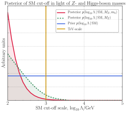
Figure 1: Distribution of $\log_{10}\Lambda$, the log of the SM cut-off. The prior distribution (blue line) was flat in $\log\Lambda$. Once conditioned upon the weak scale ($M_{Z}^{\text{exp}}$), the posterior distribution (green dashed line, filled) favors a small SM cut-off. This is the gist of the SM hierarchy problem caused by quadratic corrections, $\Lambda^{2}$. Further conditioning upon $m_{h}$ makes little difference (red line, filled). A cut-off of $\Lambda=1\,\text{TeV}$ is shown for reference by the vertical (yellow) line.

This is illustrated in Fig. 1 where this posterior distribution and a similar one from a calculation that includes the Higgs boson mass $m_{h}^{\text{exp}}\simeq 125\,\text{GeV}$ in the likelihood are plotted as functions of $\log\Lambda$. We find, as expected, that the application of Bayes’ theorem captures the gist of the hierarchy problem: quadratic corrections in the SM Higgs mass mean that we ought to expect new physics close to the measured weak scale. The prior distribution for the magnitude of the cut-off was flat, but once conditioned upon the weak scale (i.e., measurements of the $Z$-boson mass and the Higgs mass), a sub-TeV SM cut-off was favored.

Finally, we calculate $\mathcal{Z}$, the evidence of the SM in light of the measurement of $M_{Z}$, by integrating Eq. (19) with respect to the SM cut-off and rearranging to find the evidence, $\mathcal{Z}$. We find that if the lower limit on the prior for $\Lambda$ is $\Lambda_{\text{SM}}$ and $\Lambda_{\text{SM}}\gg M_{Z}^{\text{exp}}$, then

$$p(\log M_{Z}^{\text{exp}}\,\bm{|}\,\text{SM})\approx p(\log M_{Z}^{\text{exp}},\log m_{h}^{\text{exp}}\,\bm{|}\,\text{SM})\approx c\left(\frac{M_{Z}^{\text{exp}}}{\Lambda_{\text{SM}}}\right)^{2},$$ (21)

where $c$ is a coefficient determined by factors from integration and priors, which we calculated to be $\mathcal{O}(1)$ for our choices. For comparison with dimensionless fine-tuning ratios, we expressed the evidences as e.g., $p(\log M_{Z}^{\text{exp}}\,\bm{|}\,\text{SM})=M_{Z}^{\text{exp}}p(M_{Z}^{\text{exp}}\,\bm{|}\,\text{SM})$.

This tells us that if the cut-off is of the order of the Planck scale, $M_{\text{Pl}}$, then the evidence is very small, ${\mathcal{O}}(10^{-34})$. But if the model allows the cut-off to be of order $M_{Z}$ then the evidence is $\mathcal{O}(1)$. Therefore the evidence strongly prefers an SM effective theory that is valid only up to the electroweak or TeV scale (with new physics such as supersymmetry appearing at that scale) to an SM effective theory with no new physics below $M_{\text{Pl}}$. This is the essence of the well-known hierarchy problem, but expressed in a statistically rigorous manner.

Besides its coherency and connection to statistics, an advantage of this formulation over ad-hoc fine-tuning measures is that the evidence calculation can be repeated in any new extension of the SM, and consistently compared to the evidence computed in other models. If there is no cancellation of the quadratic divergences within that model then one should obtain a similar result as obtained in the toy example. In supersymmetry the quadratic divergences are cancelled; however, soft-breaking introduces corrections of order $m_{\text{SUSY}}^{2}$, which may result in fine-tuning if $m_{\text{SUSY}}\gg M_{Z}$.

In supersymmetry the quadratic divergences are cancelled; however, soft-breaking introduces corrections of the order of the squared soft masses, which may result in fine-tuning if these soft masses are required to be substantially larger than $M_{Z}$. For this reason one should expect that in supersymmetric models a similar result approximately holds, i.e.,

$$p(\log M_{Z}^{\text{exp}}\,\bm{|}\,\text{SUSY})\approx p(\log M_{Z}^{\text{exp}},\log m_{h}^{\text{exp}}\,\bm{|}\,\text{SUSY})\approx c\left(\frac{M_{Z}^{\text{exp}}}{m_{\text{SUSY}}}\right)^{2},$$ (22)

where in this expression $m_{\text{SUSY}}$ characterizes the minimal size of the soft masses consistent with the likelihood and chosen priors. We now explicitly repeat our calculations in two supersymmetric models to see whether this is the case.

4 Supersymmetric models

4.1 Models

We consider two models: a semi-constrained NMSSM and the constrained MSSM (CMSSM). The models are tractable examples of a minimal supersymmetric model and a singlet extension that we investigate with Bayesian statistics.

4.1.1 Semi-constrained NMSSM

The NMSSM solves the $\mu$-problem[132] of the MSSM by replacing the MSSM superpotential term $\mu\hat{H}_{d}\cdot\hat{H}_{u}$ by one of the form $\lambda\hat{S}\hat{H}_{d}\cdot\hat{H}_{u}$, where $\hat{S}$ is a new gauge singlet superfield. An effective $\mu$-term, given by

$$\mu_{\text{eff.}}=\lambda\langle S\rangle,$$ (23)

is then generated when the scalar component $S$ of this singlet superfield develops a vacuum expectation value (VEV), $\langle S\rangle$. The most general renormalizable superpotential of the NMSSM should also contain additional terms beyond those found in the MSSM involving the singlet $\hat{S}$. Here we restrict our attention to the $\mathbb{Z}_{3}$-conserving NMSSM (see e.g., Ref.[33, 34]), for which the full superpotential is

$$\hat{W}_{\text{NMSSM}} =y^{u}_{ij}\hat{u}^{c}_{i}\hat{H}_{u}\cdot\hat{Q}_{j}+y^{d}_{ij}\hat{d}^{c}_{i}\hat{Q}_{j}\cdot\hat{H}_{d}+y^{e}_{ij}\hat{e}^{c}_{i}\hat{L}_{j}\cdot\hat{H}_{d}+\lambda\hat{S}\hat{H}_{d}\cdot\hat{H}_{u}+\frac{1}{3}\kappa\hat{S}^{3}$$ (24)

$$=\hat{W}_{\text{MSSM}}|_{\mu=0}+\lambda\hat{S}\hat{H}_{d}\cdot\hat{H}_{u}+\frac{1}{3}\kappa\hat{S}^{3}.$$

Here the notation $\hat{W}_{\text{MSSM}}|_{\mu=0}$ refers to the usual MSSM superpotential, i.e.,

$$\hat{W}_{\text{MSSM}}=y^{u}_{ij}\hat{u}^{c}_{i}\hat{H}_{u}\cdot\hat{Q}_{j}+y^{d}_{ij}\hat{d}^{c}_{i}\hat{Q}_{j}\cdot\hat{H}_{d}+y^{e}_{ij}\hat{e}^{c}_{i}\hat{L}_{j}\cdot\hat{H}_{d}+\mu\hat{H}_{d}\cdot\hat{H}_{u},$$ (25)

evaluated with $\mu=0$. The cubic singlet coupling $\kappa$ is required to explicitly break a global $U(1)$ Peccei-Quinn symmetry, which would otherwise give rise to a massless axion when it is spontaneously broken by the scalar field $S$ acquiring a VEV.

As usual in phenomenological SUSY models, in the NMSSM SUSY is softly broken by a set of explicit soft terms,

$$\mathcal{L}_{\text{soft}}^{\text{NMSSM}}=\mathcal{L}_{\text{soft-scalar}}+\mathcal{L}_{\text{soft-gaugino}}+\mathcal{L}_{\text{soft-trilinear}},$$ (26)

where the soft scalar masses, gaugino masses and soft trilinear terms are taken to be

$$-\mathcal{L}_{\text{soft-scalar}} =m^{2}_{S}|S|^{2}+m_{H_{u}}^{2}|H_{u}|^{2}+m_{H_{d}}^{2}|H_{d}|^{2}+m_{Q_{ij}}^{2}\tilde{Q}^{\dagger}_{i}\tilde{Q}_{j}$$

$$\quad{}+m_{u^{c}_{ij}}^{2}\tilde{u}^{c\,\dagger}_{i}\tilde{u}^{c}_{j}+m_{d^{c}_{ij}}^{2}\tilde{d}^{c\,\dagger}_{i}\tilde{d}^{c}_{j}+m_{L_{ij}}^{2}\tilde{L}^{\dagger}_{i}\tilde{L}_{j}+m_{e^{c}_{ij}}^{2}\tilde{e}^{c\,\dagger}_{i}\tilde{e}^{c}_{j},$$ (27)

$$-\mathcal{L}_{\text{soft-gaugino}} =\frac{1}{2}(M_{1}\tilde{B}\tilde{B}+M_{2}\tilde{W}\tilde{W}+M_{3}\tilde{g}\tilde{g}+\text{h.c.}),$$ (28)

$$-\mathcal{L}_{\text{soft-trilinear}} =a^{u}_{ij}\tilde{u}^{c}_{i}H_{u}\cdot\tilde{Q}_{j}+a^{d}_{ij}\tilde{d}^{c}_{i}\tilde{Q}_{j}\cdot H_{d}+a^{e}_{ij}\tilde{e}^{c}_{i}\tilde{L}_{j}\cdot H_{d}$$

$$\quad{}+a_{\lambda}SH_{d}\cdot H_{u}+\frac{1}{3}a_{\kappa}S^{3}+\text{h.c.},$$ (29)

respectively. To construct the semi-constrained NMSSM that we consider here, the above soft parameters are assumed to satisfy a set of relationships at the grand unification (GUT) scale $M_{\text{GUT}}$ motivated by those found in minimal supergravity (mSUGRA)[133, 134]. These GUT scale boundary conditions are as follows:

• The soft-breaking trilinears are parameterized by

  $$\begin{gathered}a^{u}_{ij}(M_{\text{GUT}})\equiv y^{u}_{ij}(M_{\text{GUT}})A^{u}_{ij},\,a^{d}_{ij}(M_{\text{GUT}})\equiv y^{d}_{ij}(M_{\text{GUT}})A^{d}_{ij},\,a^{e}_{ij}(M_{\text{GUT}})\equiv y^{e}_{ij}(M_{\text{GUT}})A^{e}_{ij},\\ a_{\lambda}(M_{\text{GUT}})\equiv\lambda(M_{\text{GUT}})A_{\lambda},\text{ and }a_{\kappa}(M_{\text{GUT}})\equiv\kappa(M_{\text{GUT}})A_{\kappa},\end{gathered}$$ (30)

  where the reduced trilinear couplings are partially unified at the GUT scale, that is,

  $$A^{u}_{ij}=A^{d}_{ij}=A^{e}_{ij}\equiv A_{0}\delta_{ij},$$ (31)

  while $A_{\lambda}$ and $A_{\kappa}$ are allowed to vary separately.

• The soft-breaking scalar masses are partially unified at $M_{\text{GUT}}$,

  $$\begin{gathered}m^{2}_{Q_{ij}}(M_{\text{GUT}})=m^{2}_{L_{ij}}(M_{\text{GUT}})=m^{2}_{u^{c}_{ij}}(M_{\text{GUT}})=m^{2}_{d^{c}_{ij}}(M_{\text{GUT}})=m^{2}_{e^{c}_{ij}}(M_{\text{GUT}})\equiv m_{0}^{2}\delta_{ij},\\ m_{H_{d}}^{2}(M_{\text{GUT}})=m_{H_{u}}^{2}(M_{\text{GUT}})\equiv m_{0}^{2}.\end{gathered}$$ (32)

  The exception is the soft-breaking scalar mass for the singlet, $m_{S}^{2}(M_{\text{GUT}})\equiv m_{S_{0}}^{2}$, which is taken to be free.

• The soft-breaking gaugino masses are unified at the GUT scale,

  $$M_{1}(M_{\text{GUT}})=M_{2}(M_{\text{GUT}})=M_{3}(M_{\text{GUT}})\equiv m_{1/2}.$$ (33)

In addition to the GUT scale values of the soft parameters, the values of the Yukawa couplings $\lambda$ and $\kappa$ at the GUT scale, $\lambda(M_{\text{GUT}})\equiv\lambda_{0}$ and $\kappa(M_{\text{GUT}})\equiv\kappa_{0}$, must also be specified. This semi-constrained model is therefore described by the nine GUT scale parameters

$$\{A_{0},A_{\lambda},A_{\kappa},m_{0},m_{S_{0}}^{2},m_{1/2},\lambda_{0},\kappa_{0},\text{sign}\,\mu_{\text{eff.}}\}.$$ (34)

In the MSSM, the effects of $A$ terms are absorbed into the RG evolution of the soft terms such that the VEVs have no explicit dependence on them. On the other hand, the VEVs depend on $A$ terms directly in the NMSSM. It is, therefore, important to have flexible constraints on $A$ terms in the semi-constrained NMSSM.

Note that, depending on the literature, the semi-constrained NMSSM is defined by slightly different assumptions. A more strict convention allows only the singlet specific parameters to be unconstrained such that $A_{\lambda}=A_{0}$ is implied at the GUT scale[37], while the more flexible version lets non-universal Higgs masses be free parameters as well as $A_{\lambda}$ [135].

Hereafter, NMSSM is used to simply denote the semi-constrained NMSSM, if there is no special reason to distinguish it from the general NMSSM.

4.1.2 CMSSM

For comparison purposes we use the CMSSM [133, 134, 136], one of the most-studied supersymmetric models. In the parameterization that we consider, the model can be characterized by five parameters at the GUT scale. These are a common scalar mass, $m_{0}$, a common gaugino mass, $m_{1/2}$, a common trilinear, $A_{0}$, the GUT scale value of the $\mu$ parameter appearing in Eq. (25), $\mu_{0}\equiv\mu(M_{\text{GUT}})$, and the GUT scale value of the corresponding soft-breaking bilinear coupling, $B_{0}\mu_{0}\equiv B\mu(M_{\text{GUT}})$, where $\mathcal{L}_{\text{soft}}^{\text{MSSM}}\supset B\mu(H_{d}\cdot H_{u}+\text{h.c.})$. The unified soft parameters $m_{0}$, $m_{1/2}$, and $A_{0}$ have analogous definitions to those used in the semi-constrained NMSSM; that is, in the CMSSM the boundary conditions Eq. (31), Eq. (32), and Eq. (33) are assumed to hold.

4.2 Likelihood and priors

We include Particle Data Group (PDG) world-averages[1] of measurements of the Higgs and $Z$-boson masses in Table 1 in our likelihood function. Under integration, we approximate the Gaussian likelihood function for the $Z$-boson mass by a Dirac $\delta$-function, as in Eq. (12). We added in quadrature a $1\,\text{GeV}$ theoretical uncertainty in the calculation of the SM-like Higgs boson mass by SOFTSUSY [137, 138].

Parameter	PDG	Theory error	Distribution
$M_{Z}$	$91.1876\pm 0.0021\,\text{GeV}$[1]		Dirac
$m_{h}$	$125.09\pm 0.24\,\text{GeV}$[1]	$1\,\text{GeV}$	Gaussian

Table 1: Likelihoods in our analysis for the Higgs and $Z$-boson masses. We added in quadrature a $1\,\text{GeV}$ theory error upon the SOFTSUSY calculation of $m_{h}$.

Our chosen priors for the parameters of the CMSSM and the semi-constrained NMSSM are shown in Table 2. Because we are ignorant of the soft-breaking mass scale, we pick logarithmic priors, where possible, that equally weight every order of magnitude. Note that the trilinear couplings in both models, $A_{0}$, $A_{\lambda}$, and $A_{\kappa}$, are allowed to take both signs, and we use the piecewise prior

$$p(A)\propto\begin{cases}1&|A|\leq 100\,\text{GeV},\\ \frac{100\,\text{GeV}}{|A|}&100\,\text{GeV}<|A|\leq 20\,\text{TeV},\\ 0&|A|>20\,\text{TeV}.\\ \end{cases}$$ (35)

This choice corresponds to a logarithmic prior with special treatment at $|A|\simeq 0$ such that the prior remains proper.

In addition to the relevant GUT scale parameters, the models share nuisance parameters that are not of particular interest in this analysis, but which could impact our results. The most important nuisance parameters are the top quark mass, $m_{t}^{\text{pole}}$, and the strong coupling, $\alpha_{s}(M_{Z})^{\overline{\text{MS}}}$. We pick Gaussian priors for them, with means and standard deviations determined by PDG world-averages of experimental measurements[1], as shown in Table 2. We fix other SM nuisance parameters, including the bottom mass and weak coupling, to their measured values.

Parameter	Distribution
CMSSM
$m_{0}$	Log, $1\,\text{GeV}\text{, }20\,\text{TeV}$
$m_{1/2}$	Log, $1\,\text{GeV}\text{, }15\,\text{TeV}$
$A_{0}$	Log for $100\,\text{GeV}<|A|\leq 20\,\text{TeV}$, Flat for $|A|\leq 100\,\text{GeV}$
$|\mu_{0}|$	Log, $100\,\text{GeV}\text{, }20\,\text{TeV}$
$B_{0}\mu_{0}$	Log, $(100\,\text{GeV})^{2}\text{, }(20\,\text{TeV})^{2}$
$\text{sign}\,\mu$	$\pm 1$ with equal probability
NMSSM
$\lambda_{0}$	Log, $10^{-6}\text{, }1$
$\kappa_{0}$	Log for $10^{-10}<|\kappa|<1$
$m_{S_{0}}$	Same as $m_{0}$
$A_{\lambda}$	Same as $A_{0}$
$A_{\kappa}$	Same as $A_{0}$
SM
$\alpha_{s}(M_{Z})^{\overline{\text{MS}}}$	Gaussian, $0.1185\pm 0.0006$[1]
$m_{t}^{\text{pole}}$	Gaussian, $173.34\pm 0.76\,\text{GeV}$[1]

Table 2: Priors for the CMSSM and semi-constrained NMSSM model parameters. In the CMSSM, $|\mu_{0}|$ is marginalized in accordance with $M_{Z}$, while in the NMSSM $m_{S}$ is marginalized as $|\mu_{0}|$ via $\langle S\rangle$, as described in Sec. 4.2.1. The full set of parameters in our scan of the CMSSM includes the SM parameters, and the same priors are used in the NMSSM for those parameters that are shared with the CMSSM. In the case of the NMSSM, the parameters $|\mu_{0}|$ and $B_{0}\mu_{0}$ are absent and instead we specify priors for $\lambda_{0}$ and $\kappa_{0}$.

4.2.1 Effective naturalness priors

As in the SM in Eq. (15), from these initial priors we find effective priors in the CMSSM and NMSSM in which one of the GUT scale parameters is fixed to reproduce the observed value of $M_{Z}^{2}$. This corresponds quite closely to the approach taken in spectrum generators for the MSSM and NMSSM, such as SOFTSUSY, where some of the presumed fundamental parameters are traded for phenomenological parameters at the weak scale. The models can then be parameterized in terms of the remaining GUT scale parameters and a set of precisely known electroweak (EW) parameters. It should be noted, however, that this is equivalent to working directly in terms of the GUT scale parameters and marginalizing with the chosen EW observables using a $\delta$-function likelihood. This provides an economic way to survey the entirety of parameter space, discarding points that lead to hardly justifiable low-energy spectra.

In the MSSM, the effective priors arise from making the conventional trade

$$\{|\mu_{0}|,\,B_{0}\mu_{0},\,\text{sign}\,\mu,\dots\}\to\{M_{Z}^{2},\,\tan\beta,\,\text{sign}\,\mu,\dots\},$$ (36)

where as usual $\tan\beta\equiv v_{2}/v_{1}$ is defined as the ratio of the two Higgs VEVs,

$$\langle H_{d}^{0}\rangle=\frac{v_{1}}{\sqrt{2}},\quad\langle H_{u}^{0}\rangle=\frac{v_{2}}{\sqrt{2}}.$$ (37)

In practice, we achieve this trade in two steps. First, the GUT scale parameters are evolved to $m_{\text{SUSY}}\equiv\sqrt{m_{\tilde{t}_{1}}m_{\tilde{t}_{2}}}$, the scale of EW symmetry breaking (EWSB), using two-loop renormalization group equations (RGEs). The EWSB conditions,

$$\frac{1}{2}M_{Z}^{2} =-\mu^{2}+\frac{\bar{m}^{2}_{H_{d}}-\bar{m}^{2}_{H_{u}}\tan^{2}{\beta}}{\tan^{2}{\beta}-1}-\frac{1}{2}\operatorname{Re}\Pi_{ZZ}^{T},$$ (38)

$$\sin 2\beta =\frac{2B\mu}{\bar{m}_{H_{u}}^{2}+\bar{m}_{H_{d}}^{2}+2\mu^{2}},$$ (39)

can then be used to exchange the low-energy values of $\mu$ and $B\mu$ for $M_{Z}^{2}$ and $\tan\beta$. In these expressions, the one- and two-loop corrections from the Coleman-Weinberg potential[139] have been absorbed into the quantities $\bar{m}_{H_{d,u}}^{2}$, and $\operatorname{Re}\Pi_{ZZ}^{T}$ is the transverse part of the $Z$-boson self-energy. Since the EWSB conditions cannot fix the phase of the $\mu$-parameter, $\text{sign}\,\mu$ is an additional parameter. This trade is convenient, since we may now input the measured $Z$-boson and fermion masses, the latter being related to their Yukawa couplings via $\tan\beta$.

The priors for the two choices of parameter sets are related by the Jacobian, $\mathcal{J}^{\text{\text{CMSSM}}}$, associated with this change of variables,

$$p(|\mu_{0}|,\text{sign}\,\mu,B_{0}\mu_{0},\dots\,\bm{|}\,\text{\text{CMSSM}}) \equiv p(\mu_{0},B_{0}\mu_{0},\dots\,\bm{|}\,\text{\text{CMSSM}})$$

$$=\mathcal{J}^{\text{\text{CMSSM}}}\cdot p(M_{Z}^{2},\tan\beta,\dots\,\bm{|}\,\text{\text{CMSSM}}),$$ (40)

where $\mathcal{J}^{\text{\text{CMSSM}}}$ is given by $\mathcal{J}^{\text{\text{CMSSM}}}=|\det J^{\text{\text{CMSSM}}}|$, $J^{\text{\text{CMSSM}}}$ being the appropriate Jacobian matrix. Here we treat the RG evolution from $M_{\text{GUT}}$ to $m_{\text{SUSY}}$ and the subsequent solution of the EWSB conditions as two consecutive changes of variables, so that $\mathcal{J}^{\text{\text{CMSSM}}}$ may be written as a product of the Jacobian determinant associated with each, i.e.,

$$\mathcal{J}^{M}=\mathcal{J}^{M}_{m_{\text{SUSY}}}\mathcal{J}^{M}_{M_{\text{GUT}}},$$ (41)

where $M=\text{\text{CMSSM}},\text{NMSSM}$ denotes the particular model under consideration. The forms of $\mathcal{J}^{M}_{m_{\text{SUSY}}}$ and $\mathcal{J}^{M}_{M_{\text{GUT}}}$ are given in App. A.

The effective prior results from conditioning on the measurement of $M_{Z}$ and then marginalizing over $M_{Z}$. This yields

$$p_{\text{eff.}}(\tan\beta,\dots) =\int p(M_{Z}^{2},\tan\beta,\dots\,\bm{|}\,\text{\text{CMSSM}},M_{Z}^{\text{exp}})\mathop{}\!\mathrm{d}M_{Z}^{2}$$ (42)

$$\equiv\frac{1}{\mathcal{Z}}\int\delta((M_{Z}^{\text{exp}})^{2}-M_{Z}^{2})\cdot p(M_{Z}^{2},\tan\beta,\dots\,\bm{|}\,\text{\text{CMSSM}})\mathop{}\!\mathrm{d}M_{Z}^{2}$$

$$=\frac{1}{\mathcal{Z}}p((M_{Z}^{\text{exp}})^{2},\tan\beta,\dots\,\bm{|}\,\text{\text{CMSSM}})$$

$$=\frac{1}{\mathcal{Z}}\left.\frac{1}{\mathcal{J}^{\text{\text{CMSSM}}}}\right|_{M_{Z}^{\text{exp}}}p(\mu_{Z},B_{Z}\mu_{Z},\dots\,\bm{|}\,\text{\text{CMSSM}}),$$ (43)

where $\mu_{Z}=\mu_{0}(M_{Z}=M_{Z}^{\text{exp}})$ and $B_{Z}\mu_{Z}=B_{0}\mu_{0}(M_{Z}=M_{Z}^{\text{exp}})$ are the values of the high-scale parameters that result for $M_{Z}=M_{Z}^{\text{exp}}$, for the given value of $\tan\beta$ and all other model parameters. The form of the effective prior is identical to that in the SM in Eq. (15). It is worth noting that we do not develop any nontrivial, or misleading, behavior in the effective prior according to our choice of EW parameters, $\{M_{Z}^{2},\tan\beta\}$. This choice is not unique; for instance, one could choose the VEVs $\{v_{1},v_{2}\}$ instead. In this case, the effective prior would differ only by the additional non-singular Jacobian factor

$$\left|\det\frac{\partial(v_{1},v_{2})}{\partial(M_{Z}^{2},\tan\beta)}\right|\approx\frac{v_{1}^{2}}{2m_{Z}^{2}},$$ (44)

where $m_{Z}$ is the tree-level $Z$-boson mass.

In the NMSSM, the imposed $\mathbb{Z}_{3}$ symmetry forbids an explicit superpotential bilinear term for $\hat{H}_{d}$ and $\hat{H}_{u}$, along with the corresponding soft-breaking parameter. We instead make the trade

$$\{\lambda_{0},\kappa_{0},m_{S_{0}}^{2}\}\to\{\lambda,M_{Z}^{2},\tan\beta\}.$$ (45)

After the intermediate step of exchanging GUT scale parameters for their low-energy counterparts through RG running, we can make use of the three NMSSM EWSB conditions to obtain the new set of input parameters. Note that exchanging $\lambda_{0}$ for $\lambda$ is achieved solely by integrating the RGEs, so that at the EWSB scale we need only trade $\{\kappa,m_{S}^{2}\}\to\{M_{Z}^{2},\tan\beta\}$.

To do so, we first use the MSSM-like EWSB condition

$$\frac{1}{2}M_{Z}^{2}=-\mu_{\text{eff.}}^{2}+\frac{\bar{m}^{2}_{H_{d}}-\bar{m}^{2}_{H_{u}}\tan^{2}{\beta}}{\tan^{2}{\beta}-1}-\frac{1}{2}\operatorname{Re}\Pi_{ZZ}^{T},$$ (46)

where the effective $\mu$-parameter, $\mu_{\text{eff.}}$, is defined in Eq. (23), to express the effective $\mu$-parameter in terms of $M_{Z}^{2}$ and $\tan\beta$. Since in this approach we retain $\lambda$ as a free input parameter, this has the effect of determining the singlet VEV, $\langle S\rangle\equiv s/\sqrt{2}$, as a function of $M_{Z}^{2}$ and $\tan\beta$.

Second, we trade $s$ for $m_{S}^{2}$ via the EWSB condition,

$$\bar{m}_{S}^{2}=-\kappa^{2}s^{2}-\frac{1}{2}\lambda^{2}v^{2}-\frac{a_{\kappa}s}{\sqrt{2}}+\frac{v^{2}}{2s}\sin 2\beta\left(\frac{a_{\lambda}}{\sqrt{2}}+\lambda\kappa s\right),$$ (47)

where we make the usual definition $v^{2}=v_{1}^{2}+v_{2}^{2}$, and have absorbed the loop-corrections from the Coleman-Weinberg potential into $\bar{m}_{S}^{2}$. Finally, we make $\tan\beta$ an input parameter by trading $\kappa$ for $\tan\beta$ via the second MSSM-like EWSB condition,

$$\sin 2\beta=\frac{2B_{\text{eff.}}\mu_{\text{eff.}}}{\bar{m}_{H_{u}}^{2}+\bar{m}_{H_{d}}^{2}+2\mu_{\text{eff.}}^{2}+\frac{\lambda^{2}v^{2}}{2}},$$ (48)

where we define an effective soft-breaking bilinear

$$B_{\text{eff.}}\mu_{\text{eff.}}\equiv\frac{s}{\sqrt{2}}\left(a_{\lambda}+\frac{\lambda\kappa s}{\sqrt{2}}\right).$$ (49)

Thus, ultimately, in our analysis $m_{S}^{2}$ plays the role of $\mu^{2}$ via an effective $\mu$-term and $\kappa$ plays the role of $B\mu$ via an effective $B\mu$-term. The final effective prior is defined in the same way as in the CMSSM, i.e., it has the form

$$p_{\text{eff.}}(\tan\beta,\lambda,\dots)=\frac{1}{\mathcal{Z}}\left.\frac{1}{\mathcal{J}^{\text{NMSSM}}}\right|_{M_{Z}^{\text{exp}}}p(\lambda_{Z},\kappa_{Z},m_{S_{Z}}^{2}\dots\,\bm{|}\,\text{NMSSM}).$$ (50)

The effective priors automatically disfavor fine-tuned regions of parameter space. Indeed, from their explicit forms in App. A, we see that the effective priors favor RG evolution that results in weak-scale parameters similar in magnitude to the weak scale. The region of parameter space in which this occurs is known as the “focus point”[140, 141, 142]. In these regions of parameter space, the RG evolution of the soft masses is such that, at the SUSY scale, $m_{H_{u}}^{2}\sim M_{Z}^{2}$ almost independently of the initial value of $m_{H_{u}}^{2}(M_{\text{GUT}})=m_{0}^{2}$. In the CMSSM, the dependence of $m_{H_{u}}^{2}(m_{\text{SUSY}})$ on the universal soft-breaking masses can be quantified using semi-analytic solutions to the RGEs, which take the form

$$m^{2}(m_{\text{SUSY}}) =c^{m^{2}}_{m_{0}^{2}}(m_{\text{SUSY}})m_{0}^{2}+c^{m^{2}}_{m_{1/2}^{2}}(m_{\text{SUSY}})m_{1/2}^{2}+c^{m^{2}}_{m_{1/2}A_{0}}(m_{\text{SUSY}})m_{1/2}A_{0}$$

$$\quad{}+c^{m^{2}}_{A_{0}^{2}}(m_{\text{SUSY}})A_{0}^{2},$$ (51)

for $m^{2}=m_{H_{u}}^{2},m_{H_{d}}^{2}$ and where the coefficients $c^{i}_{j}(Q)$ depend only on the gauge and Yukawa couplings. In the semi-constrained NMSSM the semi-analytic solutions instead take the form

$$m^{2}(m_{\text{SUSY}}) =c^{m^{2}}_{m_{0}^{2}}(m_{\text{SUSY}})m_{0}^{2}+c^{m^{2}}_{m_{S_{0}}^{2}}(m_{\text{SUSY}})m_{S_{0}}^{2}+c^{m^{2}}_{m_{1/2}^{2}}(m_{\text{SUSY}})m_{1/2}^{2}$$

$$\quad{}+c^{m^{2}}_{m_{1/2}A_{0}}(m_{\text{SUSY}})m_{1/2}A_{0}+c^{m^{2}}_{m_{1/2}A_{\lambda}}(m_{\text{SUSY}})m_{1/2}A_{\lambda}$$

$$\quad{}+c^{m^{2}}_{m_{1/2}A_{\kappa}}(m_{\text{SUSY}})m_{1/2}A_{\kappa}+c^{m^{2}}_{A_{0}A_{\lambda}}(m_{\text{SUSY}})A_{0}A_{\lambda}+c^{m^{2}}_{A_{0}A_{\kappa}}(m_{\text{SUSY}})A_{0}A_{\kappa}$$

$$\quad{}+c^{m^{2}}_{A_{\lambda}A_{\kappa}}(m_{\text{SUSY}})A_{\lambda}A_{\kappa}+c^{m^{2}}_{A_{0}^{2}}(m_{\text{SUSY}})A_{0}^{2}+c^{m^{2}}_{A_{\lambda}^{2}}(m_{\text{SUSY}})A_{\lambda}^{2}$$

$$\quad{}+c^{m^{2}}_{A_{\kappa}^{2}}(m_{\text{SUSY}})A_{\kappa}^{2}$$ (52)

for $m^{2}=m_{H_{u}}^{2},m_{H_{d}}^{2},m_{S}^{2}$.

4.3 Comparison to other fine-tuning measures

As discussed in Sec. 2 and Sec. 3, Bayesian methods automatically incorporate some of the common intuitions relating to fine-tuning. It is therefore useful to compare the results obtained in the Bayesian approach to other measures of tuning. The traditional sensitivity measure defined in Eq. (8) is one example. In addition to the ambiguities related to this measure discussed in Sec. 3, there is also no agreement as to how a collection of sensitivities $\{\Delta_{p}\}$ should be calculated or combined to produce a tuning measure. For instance, it is not necessarily clear whether the sensitivities should be summed, profiled, added in quadrature, or combined in some other way, nor is there agreement on the renormalization scale of the parameters with respect to which we differentiate $M_{Z}$. For our purposes, we define

$$\Delta_{\text{BG}}\equiv\max_{p}\Delta_{p}\big{|}_{M_{\text{GUT}}},$$ (53)

where $\Delta_{p}$ is defined as in Eq. (8) and the notation $\Delta_{p}\big{|}_{Q}$ indicates that the parameters to differentiate with respect to are those defined at the scale $Q$; here, this is taken to be $Q=M_{\text{GUT}}$, the scale of gauge coupling unification. In the CMSSM, we pick the maximum from the measures for the parameters $\{A_{0},m_{0},m_{1/2},\mu_{0},B_{0}\mu_{0}\}$. In the NMSSM, on the other hand, we consider $\{A_{0},A_{\lambda},A_{\kappa},m_{0},m_{S_{0}}^{2},m_{1/2},\lambda_{0},\kappa_{0}\}$.

The BGEN measure defined in Eq. (53) identifies fine-tuning with sensitivity to small parameter variations. Alternative naturalness measures have been proposed that instead seek to quantify the size of any cancellations that must take place to reproduce the observed EW scale. An example of this class of measures is the so-called electroweak fine-tuning[143], which is defined as

$$\Delta_{\text{EW}}\equiv\max_{i}\frac{|C_{i}|}{m_{Z}^{2}/2}.$$ (54)

The $C_{i}$ are the terms appearing in the expression for $m_{Z}^{2}$ in the model (see Eq. (38) and Eq. (46)), evaluated at the renormalization scale $Q=m_{\text{SUSY}}$. The expressions for the $C_{i}$ appropriate to each of the CMSSM and NMSSM are given in App. B.

The measures in Eq. (53) and Eq. (54) are pointwise measures that can be compared with the (marginalized) posterior densities obtained in a complete Bayesian analysis. Evaluating the latter in general involves calculating non-trivial evidence integrals over the full model parameter space. However, even without carrying out the full computation, it can be seen that doing so nevertheless involves a simple pointwise tuning measure involving the Jacobian for the change of variables from parameters to observables. Regions of parameter space for which this quantity is large are penalized by a factor of $1/\mathcal{J}$ in evidence integrals; that is, the effective prior in such regions is suppressed. This motivates the definition of the tuning measures[86]

$$\Delta_{\mathcal{J}}\big{|}_{M_{\text{GUT}}} \equiv\left|\det\frac{\partial\ln O_{i}}{\partial\ln p_{j}(M_{\text{GUT}})}\right|=\left|\frac{\prod_{j}p_{j}(M_{\text{GUT}})}{\prod_{i}O_{i}}\right|\mathcal{J}^{M},$$ (55)

$$\Delta_{\mathcal{J}}\big{|}_{m_{\text{SUSY}}} \equiv\left|\det\frac{\partial\ln O_{i}}{\partial\ln p_{j}(m_{\text{SUSY}})}\right|=\left|\frac{\prod_{j}p_{j}(m_{\text{SUSY}})}{\prod_{i}O_{i}}\right|\mathcal{J}^{M}_{m_{\text{SUSY}}}.$$ (56)

The set $\{O_{i}\}$ contains the observables for which the parameters $p_{j}$ are traded in each model, i.e., $\{M_{Z}^{2},\tan\beta\}$ in the CMSSM and $\{\lambda,M_{Z}^{2},\tan\beta\}$ in the NMSSM. The measures in Eq. (55) and Eq. (56) differ in the scales at which the parameters $p_{j}$ are defined. The first involves the parameters $p_{j}$ defined at $M_{\text{GUT}}$, namely $\{\mu_{0},B_{0}\mu_{0}\}$ in the CMSSM and $\{\lambda_{0},\kappa_{0},m_{S_{0}}^{2}\}$ in the NMSSM, and includes the effect of running from the GUT scale to low energies. Eq. (56) only involves the trade from SUSY scale parameters to observables, so that the set of $p_{j}$ is $\{\mu,B\mu\}$ in the CMSSM and $\{\lambda,\kappa,m_{S}^{2}\}$ in the NMSSM. It can be seen from the expressions in App. A that the Jacobian factors $\mathcal{J}^{M}$ and $\mathcal{J}^{M}_{m_{\text{SUSY}}}$ resemble traditional[144, 145, 146, 147, 148, 149, 150, 151, 152, 36, 153, 154, 155, 156, 157, 158, 159, 160, 161, 162, 163, 49, 164] and alternative fine-tuning measures[165, 166, 167, 168, 169, 140, 170, 171, 172, 173, 174, 175, 176, 177, 143].

In the following, we will compare the results obtained using the framework of Bayesian statistics with the fine-tuning measures defined above, and illustrate how the former can encapsulate traditional notions of naturalness. To compare parameter inference with fine-tuning measures and Bayesian statistics, in Sec. 5 we compare “heat-maps” of fine-tuning measures with posterior densities. Because the fine-tuning measures are not densities, we must compare them in a particular parameterization, and bear in mind that densities are not invariant under reparameterizations (whereas the transformation of a fine-tuning measure is ambiguous) and that densities are dimensionful (whereas fine-tuning measures are dimensionless).

To compare model selection with fine-tuning measures and Bayesian statistics, in Sec. 5 we compare Bayes factors with ratios of fine-tuning measures. The fine-tuning measure in supersymmetric models is roughly

$$\Delta\sim\frac{m_{\text{SUSY}}^{2}}{M_{Z}^{2}}.$$ (57)

By comparing with Eq. (22) we see that the evidence for a supersymmetric model (written in terms of $\log M_{Z}$) may be crudely written as

$$p(\log M_{Z}\,\bm{|}\,\text{SUSY})\sim\frac{1}{\Delta}.$$ (58)

The parametric behavior for $m_{\text{SUSY}}^{2}\gg M_{Z}^{2}$ is identical. Thus, in this case, there is reason to expect that fine-tuning measures and Bayes factors may result in similar conclusions.

4.4 Numerical methods

We computed statistical quantities — posterior densities and evidences — with MultiNestv3.10 [178, 179, 180] and plotted them with SuperPlot [181]. For the evidence integration, we modified the convergence criteria by defining the tolerance using the average likelihood of the live points, instead of the maximum. We performed two scans for each model: one with only $M_{Z}$, and one with $M_{Z}$ and $m_{h}$ in the likelihood. We scanned 10 million and 100 million points for each scan of the CMSSM and NMSSM, respectively. To calculate the likelihoods and effective priors in each model, we computed the mass spectrum and Jacobian factors for each parameter point using a modified version of SOFTSUSY-3.6.2. As described in detail in App. A, the required Jacobian is written as the product of the Jacobian determinants for the change of variables from the GUT scale parameters to the low-energy Lagrangian parameters, and for the transformation from these parameters to the derived parameters $M_{Z}^{2}$ and $\tan\beta$, so that $\mathcal{J}$ may be expressed as in Eq. (41). The particular derivatives required for the construction of $\mathcal{J}^{M}_{m_{\text{SUSY}}}$ and $\mathcal{J}^{M}_{M_{\text{GUT}}}$ are given in App. A. We implemented subroutines to evaluate these derivatives numerically in SOFTSUSY. In the case of $\mathcal{J}^{M}_{M_{\text{GUT}}}$, this is achieved by varying the high-scale model parameters at $M_{\text{GUT}}$ and calculating the resulting values of the low-energy Lagrangian parameters using the two-loop RGEs. In a similar fashion, to determine the derivatives appearing in $\mathcal{J}^{M}_{m_{\text{SUSY}}}$, we vary the low-energy Lagrangian parameters and recalculate the predicted values of $M_{Z}^{2}$ and $\tan\beta$. The underlying changes in the VEVs are found by numerically solving the EWSB conditions for $v_{1}$, $v_{2}$ and $s$ after perturbing the model parameters. Two-loop RG evolution of all the model parameters such as the soft-breaking gaugino masses, scalar masses and trilinear terms is applied for the entire calculation. One-loop threshold corrections for the gauge and Yukawa couplings are included.

For each point in our scan, we also computed the measures of fine-tuning given in Eq. (53), Eq. (54), Eq. (55) and Eq. (56). In the MSSM, we make use of the existing implementation of the BGEN measure provided by SOFTSUSY to find $\Delta_{\text{BG}}$. As analogous routines are not yet provided for the NMSSM in SOFTSUSY, we also implemented the necessary numerical calculation of $\Delta_{\text{BG}}$ in the NMSSM in our modified code. Derivatives of $M_{Z}^{2}$ are obtained numerically by perturbing the GUT scale model parameters and calculating the predicted $Z$-boson pole mass, after running to the SUSY scale and solving the EWSB conditions for the VEVs at two-loop order.

5 Results and discussion

In Fig. 2, we compare credible regions of the marginalized posterior probability density conditioned upon $M_{Z}$ (left frames) with the profiled BGEN fine-tuning measure (right frames) on the ($m_{0}$, $m_{1/2}$) planes of the CMSSM (top frames) and NMSSM (bottom frames). On the posterior density plots we show the smallest $1\sigma$ (red) and $2\sigma$ (blue) credible regions, containing $68\%$ and $95\%$ of the posterior mass respectively. On the right frames different colors trace constant contours of the profiled BGEN measure. According to the posterior plots, most probability density (that is, most of the low tuned area) lies in the weak scale valued $m_{0}$ and $m_{1/2}$ region. This not only confirms our qualitative expectations in Eq. (22), but also coincides with expectations for the scale of supersymmetry before the LHC operation. As anticipated, the BGEN measure reflects the same expectations, agreeing fairly well with the trend shown by the posterior probability. This is not a surprise considering that the dominant term in this measure appears in the posterior after trading the $\mu$ parameter to the $Z$ mass. While most of the low tuned area lies in the bulk region, which was eliminated by the LHC, parts of the focus point also feature low tuning and are still experimentally feasible. Low tuning in the focus point is prominently highlighted by the $2\sigma$ credible region of the posterior density, and supported by the BGEN measure.

The scatter plots in Fig. 2, and all other scatter plots, show points with appreciable posterior weight. The density of points results from the posterior density and the nested sampling algorithm. The CMSSM and NMSSM ($m_{0}$, $m_{1/2}$) planes feature a region with no points at $m_{0}\lesssim 100\,\text{GeV}$ and $m_{1/2}\lesssim 100\,\text{GeV}$. The CMSSM, furthermore, shows few points at $m_{1/2}\simeq 0$ and $m_{0}\simeq 250\,\text{GeV}$. Such regions are disallowed as they fail to realize a physically sensible EWSB vacuum. This problem is particularly prevalent for large $A_{0}$ and $\tan\beta$. Such regions were, moreover, ruled out prior to the LHC by LEP searches for supersymmetric particles and for the Higgs boson.

(a) CMSSM credible regions

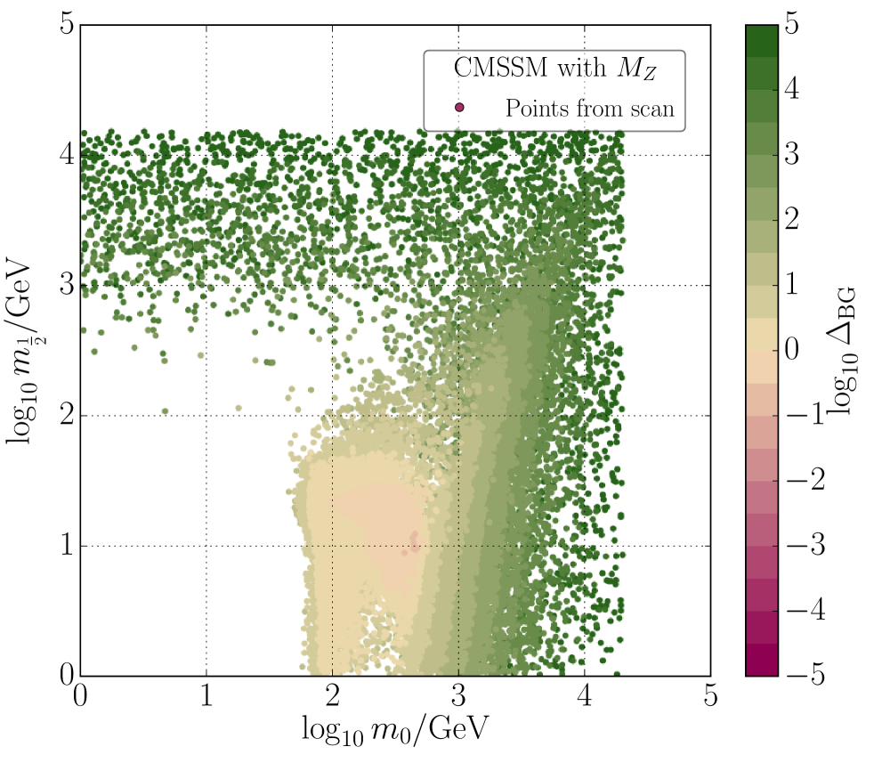
(b) CMSSM $\Delta_{\text{BG}}$

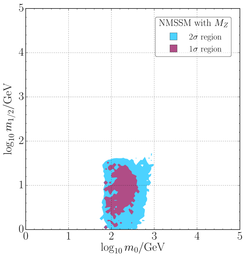
(c) NMSSM credible regions

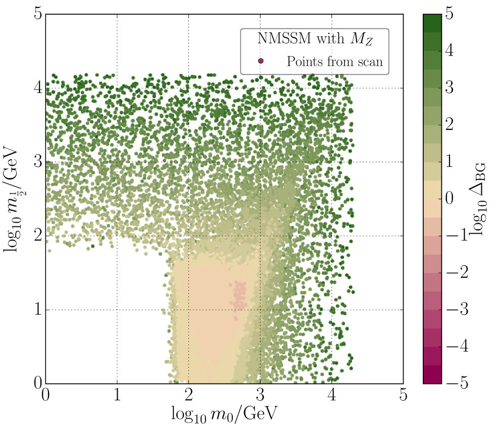
(d) NMSSM $\Delta_{\text{BG}}$

Figure 2: Credible regions of marginalized posterior probability density conditioned upon $M_{Z}$ (left) and profiled BGEN measure (right) for the CMSSM (upper) and NMSSM (lower) on the ($m_{0}$, $m_{1/2}$) plane.

Foreshadowing our inclusion of the Higgs mass in the likelihood, in Fig. 3 we show the lightest Higgs boson mass on the ($m_{0}$, $m_{1/2}$) plane for the CMSSM (left) and NMSSM (right). The color scale indicates Higgs masses from $90\,\text{GeV}$ (red) to $130\,\text{GeV}$ (green). We see that low fine-tuned regions and credible regions of the ($m_{0}$, $m_{1/2}$) plane in Fig. 2 correspond to $m_{h}\lesssim 100\,\text{GeV}$. A Higgs mass of $m_{h}\approx 125\,\text{GeV}$ requires large quantum corrections from massive sparticles and thus multi-TeV soft-breaking masses. Such points lie outside the credible regions of the posterior and are, by traditional measures, fine-tuned.

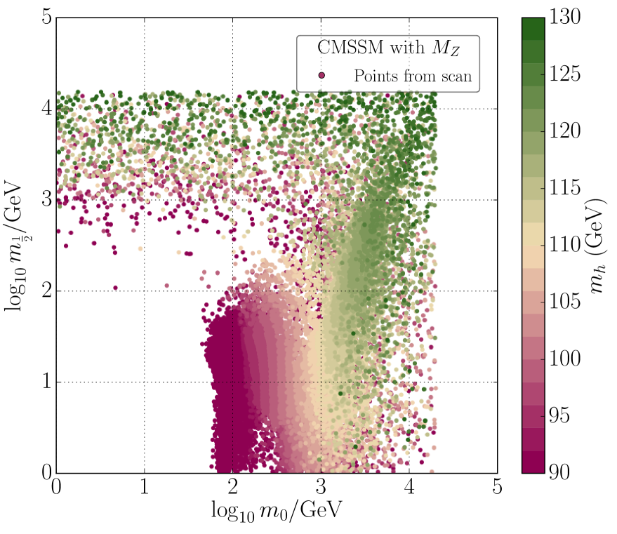
(a) CMSSM

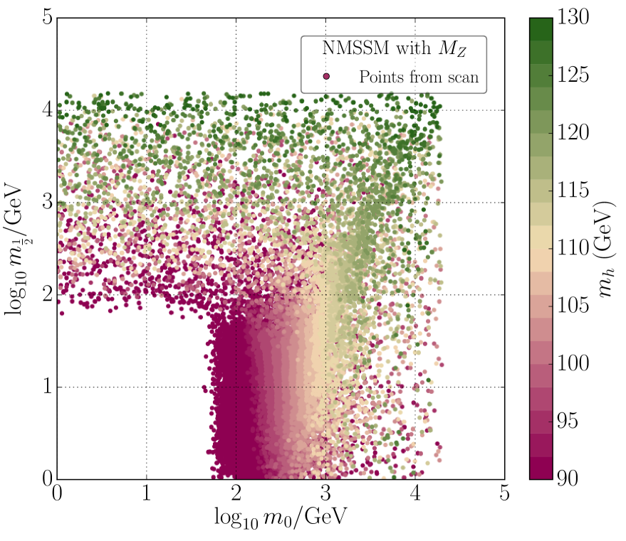
(b) NMSSM

Figure 3: The lightest Higgs mass on the ($m_{0}$, $m_{1/2}$) plane for the CMSSM (left) and NMSSM (right).

For completeness, we show the credible regions of the marginalized posterior density and the BGEN measure on the ($\tan\beta$, $A_{0}$) plane in Fig. 4. The posterior and BGEN measure agree with intuition before the LHC: $A_{0}\approx 0$, for which loop corrections to the Higgs mass are small, is natural and most plausible. As was also known in the absence of constraints on the Higgs mass, the credible regions suggest that naturalness issues are largely independent of $\tan\beta$ in the CMSSM, while they might slightly prefer low $\tan\beta$ in the NMSSM.

(a) CMSSM credible regions

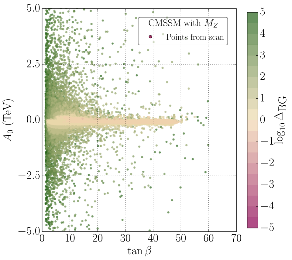
(b) CMSSM $\Delta_{\text{BG}}$

(c) NMSSM credible regions

(d) NMSSM $\Delta_{\text{BG}}$

Figure 4: Credible regions of the marginalized posterior probability density conditioned upon $M_{Z}$ (left) and profiled BGEN measure (right) for the CMSSM (upper) and NMSSM (lower) on the ($\tan\beta$, $A_{0}$) plane.

In light of our growing confidence in the posterior measuring fine-tuning, it is interesting to see how it fares against the addition of the most relevant piece of new information from the LHC: the lightest Higgs mass. This is shown in Fig. 5. Our first observation is that the most plausible regions, indicated by the $1\sigma$ and $2\sigma$ credible regions, are dramatically shifted to about two orders of magnitude higher $m_{0}$ and $m_{1/2}$ values. This is, of course, the well-known quantitative conclusion from the LHC Run 1: supersymmetry is effectively eliminated, i.e., relatively implausible, below $1\,\text{TeV}$. After folding in the lightest Higgs mass the least fine-tuned regions lie in the focus point, signalled by the slanted 1$\sigma$ region at large $m_{0}$ and $m_{1/2}$ for both the CMSSM and the NMSSM. In this region low fine tuning is achieved with relatively small values of $A_{0}$ (Fig. 6). In the vertical region spanning between $m_{1/2}$ $\sim$ 0.1-1 TeV $A_{0}$ increases with decreasing $m_{1/2}$. This still allows for acceptable fine-tuning in the CMSSM.

Just as in the case when only $M_{Z}$ was included in the likelihood, the BGEN measure confirms the picture painted by the posterior distribution. The former signals the narrow vertical region at $m_{0}\sim 10\,\text{TeV}$ and between $m_{1/2}\sim 0.1-1\,\text{TeV}$ as the least fine-tuned. This long vertical strip represents the focus point solution, thus confirming that Bayesian naturalness does find a naturalness benefit from focus point supersymmetry[140, 141, 142].

(a) CMSSM credible regions with $M_{Z}$ and $m_{h}$

(b) CMSSM $\Delta_{\text{BG}}$

(c) NMSSM credible regions with $M_{Z}$ and $m_{h}$

(d) NMSSM $\Delta_{\text{BG}}$

Figure 5: Credible regions of the marginalized posterior probability density conditioned upon $M_{Z}$ and $m_{h}$ (left), and profiled BGEN measure (right) for the CMSSM (upper) and NMSSM (lower) on the ($m_{0}$, $m_{1/2}$) plane.

(a) CMSSM credible regions

(b) CMSSM $\Delta_{\text{BG}}$

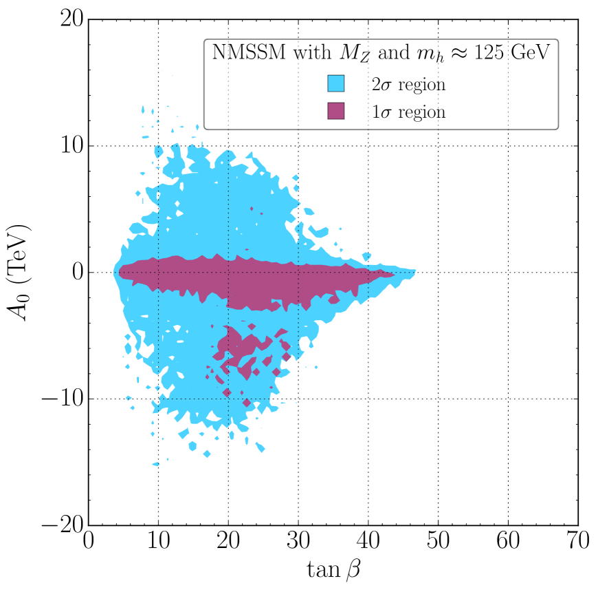
(c) NMSSM credible regions

(d) NMSSM $\Delta_{\text{BG}}$

Figure 6: Credible regions of the marginalized posterior probability density conditioned upon $M_{Z}$ and $m_{h}$ (left) and profiled BGEN measure (right) for the CMSSM (upper) and NMSSM (lower) on the ($\tan\beta$, $A_{0}$) plane.

To gauge their consistency with each other, we compare the fine-tuning measures defined in Sec. 4.3 in the CMSSM in Fig. 7 and in the NMSSM in Fig. 8 on the ($m_{0}$, $m_{1/2}$) planes. In each plot, parameters other than $m_{0}$ and $m_{1/2}$, such as $A_{0}$ and $\tan\beta$, were chosen such that the fine-tuning measure was minimized. All fine-tuning measures are qualitatively similar, with a region of low fine-tuning at $m_{\text{SUSY}}\sim M_{Z}$, and fine-tuning increases as $m_{0}$ and $m_{1/2}$ are increased, as expected. The Jacobian-based fine-tuning measures, however, are substantially smaller than the traditional BGEN measure and EW measure. We should not, however, be mislead into a superficial comparison of the measures. The Jacobian based measures, $\Delta_{\mathcal{J}}$, are volumes of multidimensional hypercubes, e.g., a two-dimensional volume in the MSSM. The BGEN measure, $\Delta_{\text{BG}}$, on the other hand, corresponds to the length of a line element and $\Delta_{\textrm{EW}}$ measures the relative size of terms contributing to $M_{Z}$.

(a) $\Delta_{\text{BG}}$

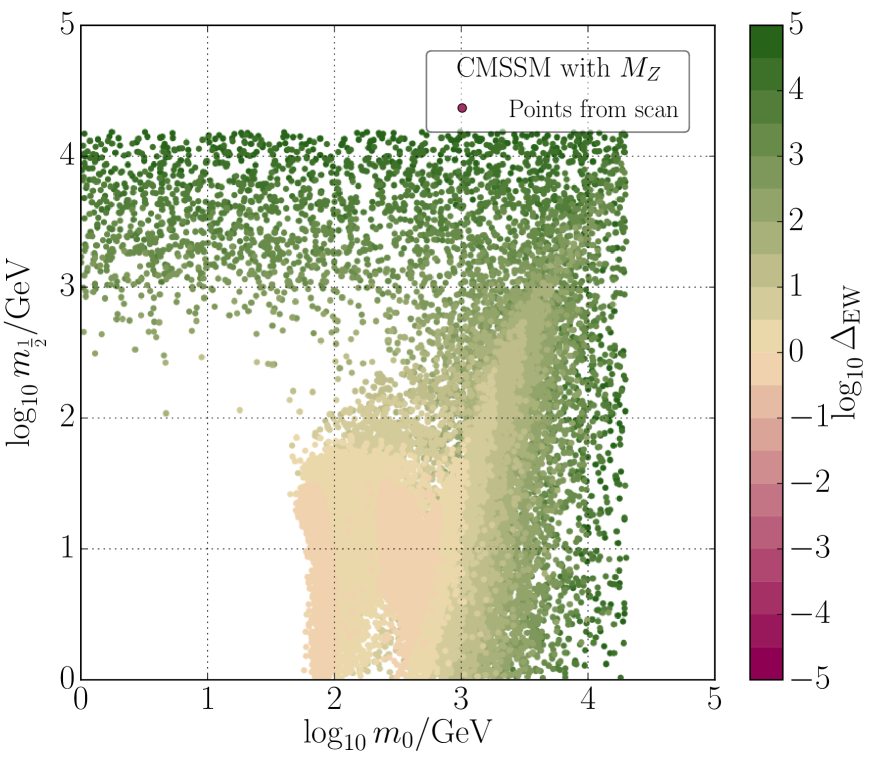
(b) $\Delta_{\text{EW}}$

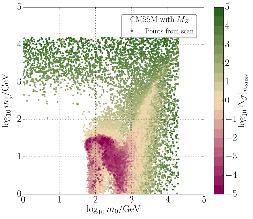
(c) $\Delta_{\mathcal{J}}\big{|}_{m_{\text{SUSY}}}$

(d) $\Delta_{\mathcal{J}}\big{|}_{M_{\text{GUT}}}$

Figure 7: Comparison of fine-tuning measures in the CMSSM on the ($m_{0}$, $m_{1/2}$) plane. For their definitions, see Sec. 4.3.

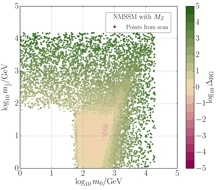
(a) $\Delta_{\text{BG}}$

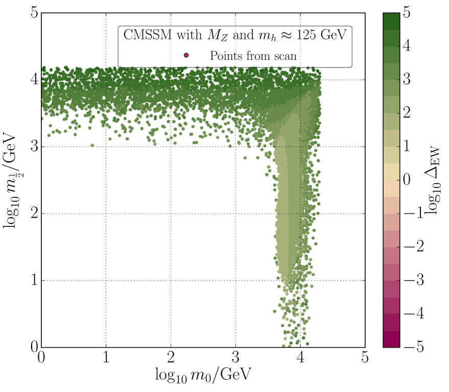
(b) $\Delta_{\text{EW}}$

(c) $\Delta_{\mathcal{J}}\big{|}_{m_{\text{SUSY}}}$

(d) $\Delta_{\mathcal{J}}\big{|}_{M_{\text{GUT}}}$

Figure 8: Comparison of fine-tuning measures in the NMSSM on the ($m_{0}$, $m_{1/2}$) plane. For their definitions, see Sec. 4.3.

Requiring that $m_{h}\simeq 125\,\text{GeV}$ increases the fine-tuning measures in the CMSSM (Fig. 9) and NMSSM (Fig. 10), and further structure is revealed. We find diagonal strips of low fine-tuning for Jacobian-based measures at about $m_{0}\sim 10\,\text{TeV}$ and $m_{1/2}\sim 1\,\text{TeV}$. The GUT scale Jacobian measure furthermore exhibits a vertical strip of low fine-tuning at $m_{0}\sim 10\,\text{TeV}$. This indicates that the Jacobian based measure has a much sharper preference for the focus point region than $\Delta_{BG}$. Note that this is the case even though we have not included the top mass or top Yukawa coupling in the set of parameters for which we take logarthmic derivatives for $\Delta_{\text{BG}}$. The Jacobian based measures in the NMSSM are also visibly smaller than those in the CMSSM.

(a) $\Delta_{\text{BG}}$

(b) $\Delta_{\text{EW}}$

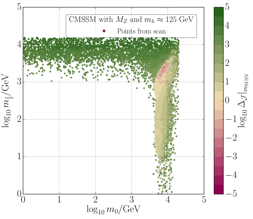
(c) $\Delta_{\mathcal{J}}\big{|}_{m_{\text{SUSY}}}$

(d) $\Delta_{\mathcal{J}}\big{|}_{M_{\text{GUT}}}$

Figure 9: Comparison of fine-tuning measures in the CMSSM with $m_{h}\approx 125\,\text{GeV}$ on the ($m_{0}$, $m_{1/2}$) plane. For their definitions, see Sec. 4.3.

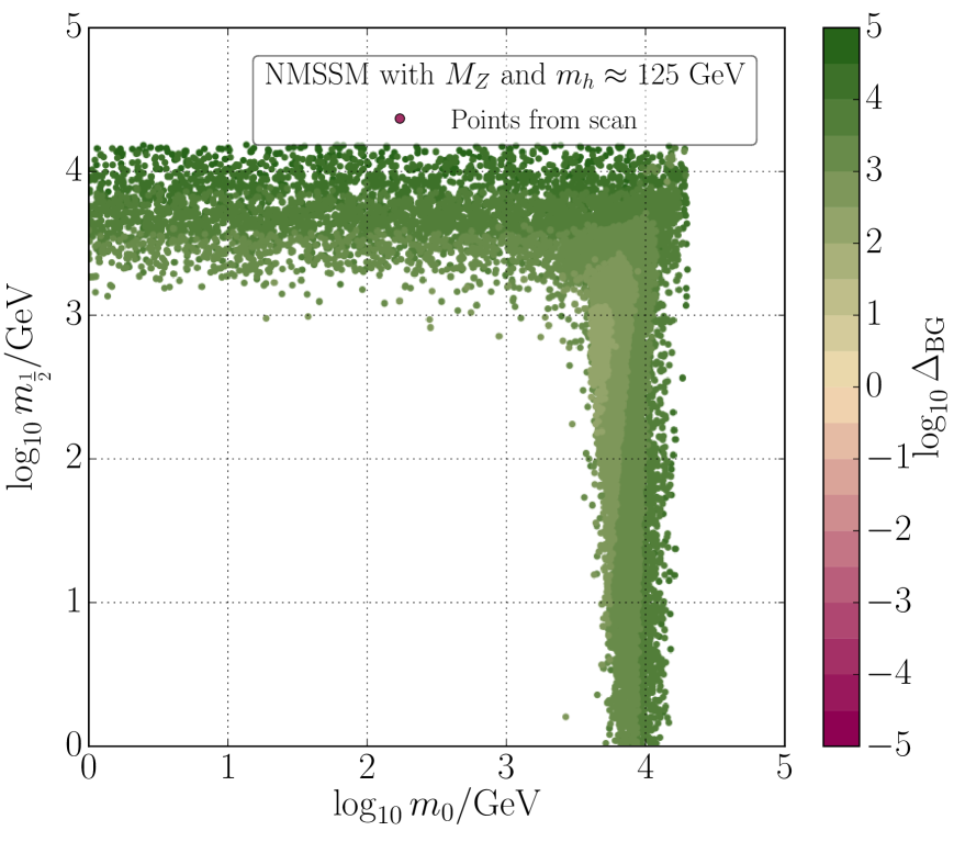
(a) $\Delta_{\text{BG}}$

(b) $\Delta_{\text{EW}}$

(c) $\Delta_{\mathcal{J}}\big{|}_{m_{\text{SUSY}}}$

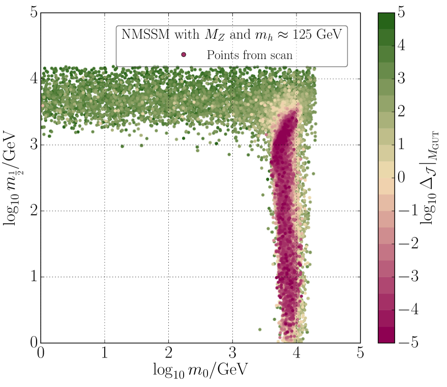
(d) $\Delta_{\mathcal{J}}\big{|}_{M_{\text{GUT}}}$

Figure 10: Comparison of fine-tuning measures in the NMSSM with $m_{h}\approx 125\,\text{GeV}$ on the ($m_{0}$, $m_{1/2}$) plane. For their definitions, see Sec. 4.3.

We summarize the one-dimensional posterior for the dimensionful parameters in Fig. 11. We see that in the CMSSM and NMSSM with only $M_{Z}$ in the likelihood, the posterior favors $m_{\text{SUSY}}\lesssim 1\,\text{TeV}$. Once we consider $M_{Z}$ and $m_{h}$, however, we require $m_{\text{SUSY}}\gtrsim 4\,\text{TeV}$ and TeV-scale soft-breaking parameters. It is, therefore, not surprising to see no signature of supersymmetric particles until the current data set of the LHC in the regard that our Higgs mass is $125\,\text{GeV}$.

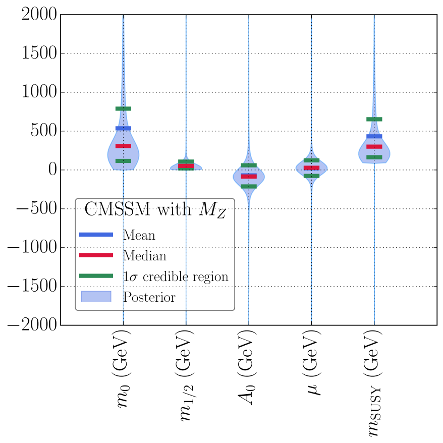
(a) CMSSM with $M_{Z}$

(b) CMSSM with $M_{Z}$ and $m_{h}$

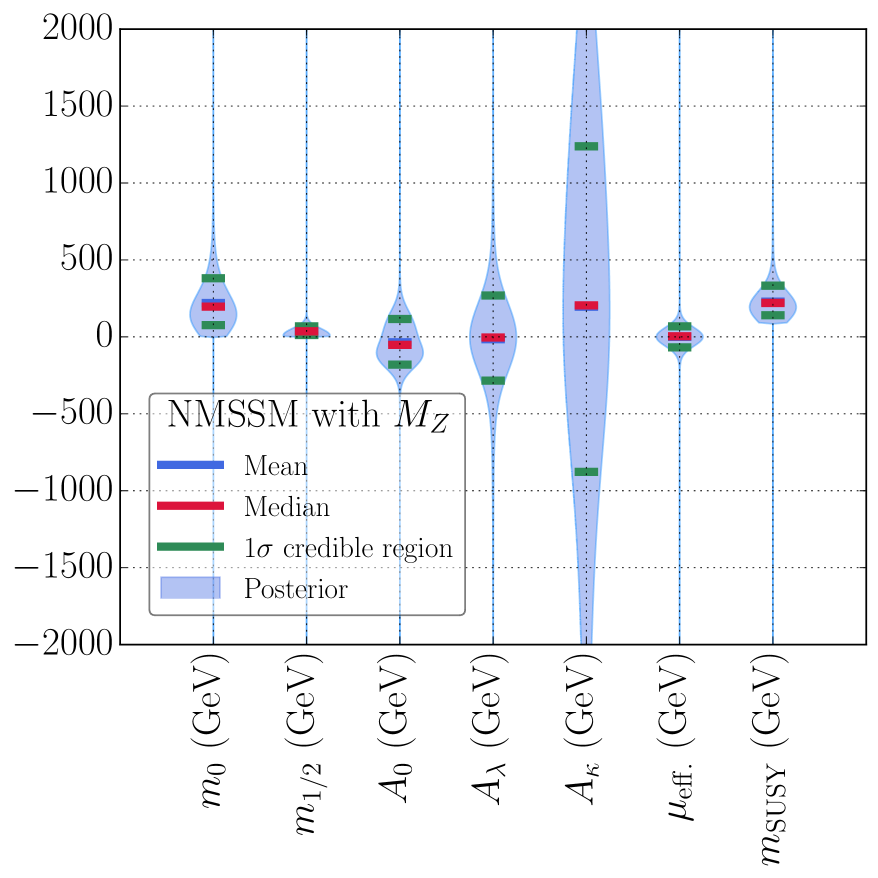
(c) NMSSM with $M_{Z}$

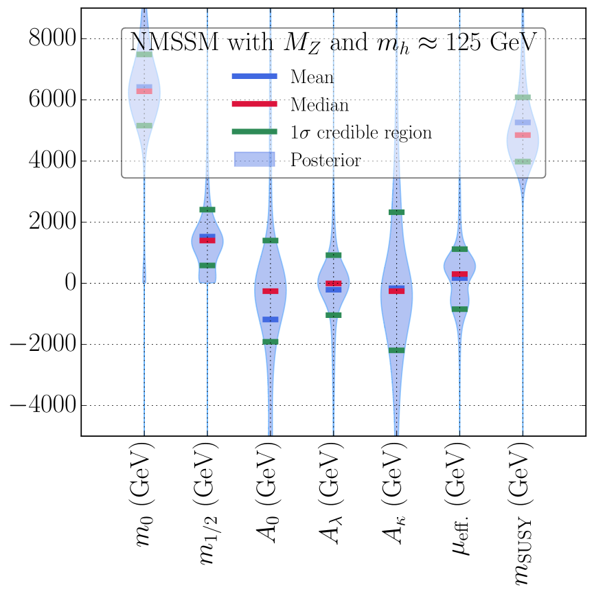
(d) NMSSM with $M_{Z}$ and $m_{h}$

Figure 11: Violin plots showing one-dimensional posterior and summary statistics for important dimensionful parameters in the CMSSM (upper) and NMSSM (lower) with only $M_{Z}$ (left) and $M_{Z}$ and $m_{h}$ (right) in the likelihood.

As a byproduct of our investigations, we calculated the Bayes factor between the semi-constrained NMSSM and CMSSM, though with appreciable uncertainty as in Ref.[82]. The Bayes factor measures the change in relative plausibility of two models in light of data. With $M_{Z}$ only, our lower estimate of the Bayes factors favored the NMSSM by a factor of about $3$, whereas our upper estimate favored it by a factor of about $20$. With $M_{Z}$ and $m_{h}$, our lower estimate favored the CMSSM by a factor of about $3$, whereas our upper estimate favored the NMSSM by a factor of about $6$. This agrees reasonably with a Bayes factor for different data calculated in Ref.[82]. The lower estimates may be more accurate as they were found by importance sampling; however, since there were significant differences between estimates from importance sampling and ordinary summation, we present our results with caution, and do not make a definitive model selection statement. To improve the accuracy of our evidence estimates requires more computational resources, or, possibly, sampling techniques which are more specialised for exploring the very strong degeneracies that can be induced by the naturalness priors in scans constrained only by measurements of $M_{Z}$ and $m_{h}$.

The minimum fine-tuning measures found in our scan are shown in Table 3. For both the CMSSM and NMSSM, we found minimum fine-tuning measures of about zero for our measures based upon the Jacobian; about $0.3$ for EW fine-tuning; and about $0.1$ for BGEN fine-tuning. If we require that $m_{h}\approx 125\,\text{GeV}$, all fine-tuning measures increase, though in this case the Jacobian-based measures and $\Delta_{\text{BG}}$ in the NMSSM are substantially less than those in the CMSSM. The EW measure, $\Delta_{\text{EW}}$, is very similar in each model. To avoid confusion, it should be stressed again that the numbers are to be compared or interpreted considering the dimensionality or the physical meaning of each measure.

	$M_{Z}$		$M_{Z}$ and $m_{h}\approx 125\,\text{GeV}$
	CMSSM	NMSSM	CMSSM	NMSSM
$\Delta_{\mathcal{J}}\big{|}_{M_{\text{GUT}}}$	${3}\times 10^{-9}$	${2}\times 10^{-10}$	0.004	${8}\times 10^{-7}$
$\Delta_{\mathcal{J}}\big{|}_{m_{\text{SUSY}}}$	${6}\times 10^{-7}$	${2}\times 10^{-10}$	0.005	${8}\times 10^{-7}$
$\Delta_{\text{EW}}$	0.3	0.3	48.7	47.4
$\Delta_{\text{BG}}$	0.1	0.2	451.9	133.2

Table 3: Minimum fine-tuning measures (defined in Sec. 4.3) found in our scans with only $M_{Z}$ in the likelihood and with the requirement that $m_{h}\approx 125\,\text{GeV}$.

6 Conclusions

After introducing fine-tuning in the context of Bayesian statistics with the Standard Model as an example, we presented a comprehensive analysis of fine-tuning in a minimal and next-to-minimal supersymmetric model. Results of a Bayesian analysis were contrasted with traditional fine-tuning measures, for parameter inference and, briefly, for model selection.

For parameter inference, conditioning upon only $M_{Z}$ we found qualitative agreement between regions favored by the posterior density and regions of low fine-tuning, as measured by, e.g., the BGEN measure. Weak-scale soft-breaking masses, i.e., $m_{\text{SUSY}}\sim M_{Z}$, were favored in a Bayesian analysis, in agreement with heuristic arguments from naturalness. This provided numerical support for our argument, made in the introduction, that naturalness arguments are underpinned by Bayesian statistics. Adding LHC measurements of the Higgs mass to our likelihood pushed the posterior for the soft-breaking masses into a multi-TeV region, as expected. This study completes our preliminary work[86] and our argument that Bayesian statistics is the correct framework for understanding fine-tuning and naturalness in supersymmetric models.

Appendix A CMSSM and NMSSM Jacobians

In this appendix we present analytic expressions for the Jacobians that appear in the effective priors as discussed in Sec. 4.2.1.

A.1 CMSSM Jacobian

In the CMSSM, the relevant Jacobian arises from making the change of variables

$$\{|\mu_{0}|,B_{0}\mu_{0}\}\to\{M_{Z}^{2},\tan\beta\}.$$ (59)

By performing this trade in two steps, namely, by first exchanging the high-scale values of the Lagrangian parameters for their values at the EW scale, and subsequently trading these for the parameters $M_{Z}^{2}$ and $\tan\beta$, the full Jacobian factorizes,

$$\mathcal{J}^{\text{\text{CMSSM}}}\equiv\mathcal{J}^{\text{CMSSM}}_{m_{\text{SUSY}}}\mathcal{J}^{\text{CMSSM}}_{M_{\text{GUT}}},$$ (60)

where the Jacobian determinants on the right-hand side arise from this series of variable changes, i.e., $\{|\mu_{0}|,B_{0}\mu_{0}\}\to\{|\mu|,B\mu\}\to\{M_{Z}^{2},\tan\beta\}$. The various prior probability density functions are related by

$$p(\mu_{0},B_{0}\mu_{0},\dots\,\bm{|}\,\text{CMSSM}) =\mathcal{J}^{\text{CMSSM}}_{M_{\text{GUT}}}p(\mu,B\mu,\dots\,\bm{|}\,\text{CMSSM})$$ (61)

$$=\mathcal{J}^{\text{CMSSM}}_{m_{\text{SUSY}}}\mathcal{J}^{\text{CMSSM}}_{M_{\text{GUT}}}p(M_{Z}^{2},\tan\beta,\dots\,\bm{|}\,\text{CMSSM}).$$ (62)

The elements of the two Jacobian matrices that are required read

$$J^{\text{CMSSM}}_{M_{\text{GUT}}}=\begin{pmatrix}\frac{\partial\mu}{\partial\mu_{0}}&\frac{\partial\mu}{\partial B_{0}\mu_{0}}\\ \frac{\partial B\mu}{\partial\mu_{0}}&\frac{\partial B\mu}{\partial B_{0}\mu_{0}}\end{pmatrix},\quad J^{\text{CMSSM}}_{m_{\text{SUSY}}}=\begin{pmatrix}\frac{\partial M_{Z}^{2}}{\partial\mu}&\frac{\partial M_{Z}^{2}}{\partial B\mu}\\ \frac{\partial\tan\beta}{\partial\mu}&\frac{\partial\tan\beta}{\partial B\mu}\end{pmatrix},$$ (63)

with $\mathcal{J}^{\text{CMSSM}}_{M_{\text{GUT}}}=|\det J^{\text{CMSSM}}_{M_{\text{GUT}}}|$ and $\mathcal{J}^{\text{CMSSM}}_{m_{\text{SUSY}}}=|\det J^{\text{CMSSM}}_{m_{\text{SUSY}}}|$.

The construction of the Jacobian matrices requires evaluating derivatives of the functions that implement the changes of variables from the initial high-scale parameters to the EW parameters. The first of these trades, $\{|\mu_{0}|,B_{0}\mu_{0}\}\to\{|\mu|,B\mu\}$, is achieved by integrating the two-loop RGEs from the GUT scale to the SUSY scale. The dependence of $\mu$ and $B\mu$ on the CMSSM parameters defined at $M_{\text{GUT}}$ can be explicitly expressed using semi-analytic solutions to the RGEs, with the result that

$$\mu(m_{\text{SUSY}}) =c^{\mu}_{\mu_{0}}(m_{\text{SUSY}})\mu_{0},$$ (64)

$$B\mu(m_{\text{SUSY}}) =c^{B\mu}_{B_{0}\mu_{0}}(m_{\text{SUSY}})B_{0}\mu_{0}+c^{B\mu}_{\mu_{0}m_{1/2}}(m_{\text{SUSY}})\mu_{0}m_{1/2}+c^{B\mu}_{\mu_{0}A_{0}}(m_{\text{SUSY}})\mu_{0}A_{0}.$$ (65)

The elements of $J^{\text{CMSSM}}_{M_{\text{GUT}}}$ can immediately be read from these expressions. The dimensionless coefficients $c^{i}_{j}$ depend only on the running of the gauge and Yukawa couplings; however, in the absence of exact analytic solutions to the two-loop RGEs they must be evaluated by numerical integration of the RGEs.

As noted in Sec. 4.2.1, the subsequent change of variables from $\{\mu,B\mu\}$ to $\{M_{Z}^{2},\tan\beta\}$ is done by solving the EWSB conditions to write the former pair as functions of $M_{Z}^{2}$ and $\tan\beta$. In the MSSM, the requirement that the neutral scalar Higgs fields acquire VEVs of the form given in Eq. (37) leads to the two EWSB conditions,

$$(\mu^{2}+m_{H_{d}}^{2})v_{1}+\frac{\bar{g}^{2}}{8}(v_{1}^{2}-v_{2}^{2})v_{1}-B\mu v_{2}-t_{1}=0,$$ (66)

$$(\mu^{2}+m_{H_{u}}^{2})v_{2}-\frac{\bar{g}^{2}}{8}(v_{1}^{2}-v_{2}^{2})v_{2}-B\mu v_{1}-t_{2}=0,$$ (67)

where

$$t_{1}=-\frac{\partial\Delta V_{\text{eff.}}^{\text{MSSM}}}{\partial v_{1}},\quad t_{2}=-\frac{\partial\Delta V_{\text{eff.}}^{\text{MSSM}}}{\partial v_{2}}$$ (68)

contain the one- and two-loop corrections to the Coleman-Weinberg potential in the MSSM. Eq. (66) and Eq. (67) define the VEVs $v_{1}$ and $v_{2}$ implicitly in terms of $\mu$ and $B\mu$, allowing the required derivatives to be written in the form

$$\begin{pmatrix}a_{11}&a_{12}\\ a_{21}&a_{22}\end{pmatrix}\begin{pmatrix}\frac{\partial v_{1}}{\partial p}\\ \frac{\partial v_{2}}{\partial p}\end{pmatrix}=\begin{pmatrix}b_{1}^{(p)}\\ b_{2}^{(p)}\end{pmatrix}$$ (69)

for $p=\mu,B\mu$. The coefficients appearing on the left-hand side of Eq. (69) are given by (assuming $\mu$ to be real)

$$a_{11} =m_{H_{d}}^{2}+\mu^{2}+\frac{\bar{g}^{2}}{8}(3v_{1}^{2}-v_{2}^{2})-\frac{\partial t_{1}}{\partial v_{1}},$$ (70)

$$a_{12} =a_{21}=-B\mu-\frac{\bar{g}^{2}}{4}v_{1}v_{2}-\frac{\partial t_{1}}{\partial v_{2}},$$ (71)

$$a_{22} =m_{H_{u}}^{2}+\mu^{2}-\frac{\bar{g}^{2}}{8}(v_{1}^{2}-3v_{2}^{2})-\frac{\partial t_{2}}{\partial v_{2}},$$ (72)

while the derivatives of the EWSB conditions with respect to the Lagrangian parameters read

$$b_{1}^{(\mu)}=-2\mu v_{1}+\frac{\partial t_{1}}{\partial\mu},\quad b_{2}^{(\mu)}=-2\mu v_{2}+\frac{\partial t_{2}}{\partial\mu},$$ (73)

$$b_{1}^{(B\mu)}=v_{2}+\frac{\partial t_{1}}{\partial B\mu},\quad b_{2}^{(B\mu)}=v_{1}+\frac{\partial t_{2}}{\partial B\mu}.$$ (74)

The elements of the Jacobian matrix $J^{\text{CMSSM}}_{m_{\text{SUSY}}}$ are then related to the solution of Eq. (69) through

$$\frac{\partial M_{Z}^{2}}{\partial p} =\left(\frac{\bar{g}^{2}v_{1}}{2}-\frac{\partial\operatorname{Re}\Pi_{ZZ}^{T}}{\partial v_{1}}\right)\frac{\partial v_{1}}{\partial p}+\left(\frac{\bar{g}^{2}v_{2}}{2}-\frac{\partial\operatorname{Re}\Pi_{ZZ}^{T}}{\partial v_{2}}\right)\frac{\partial v_{2}}{\partial p}$$

$$\quad{}-\frac{\partial\operatorname{Re}\Pi_{ZZ}^{T}}{\partial\mu}\frac{\partial\mu}{\partial p}-\frac{\partial\operatorname{Re}\Pi_{ZZ}^{T}}{\partial B\mu}\frac{\partial B\mu}{\partial p},$$ (75)

$$\frac{\partial\tan\beta}{\partial p} =\frac{1}{v_{1}}\frac{\partial v_{2}}{\partial p}-\frac{v_{2}}{v_{1}^{2}}\frac{\partial v_{1}}{\partial p},$$ (76)

for each of $p=\mu,B\mu$. In arriving at Eq. (75), we approximate the solution of

$$M_{Z}^{2}=m_{Z}^{2}-\operatorname{Re}\Pi_{ZZ}^{T}(p^{2}=M_{Z}^{2})$$

for $M_{Z}$ by evaluating the $Z$-boson self-energy at the external momentum $p^{2}=m_{Z}^{2}=\bar{g}^{2}(v_{1}^{2}+v_{2}^{2})/4$. Although it is possible to evaluate the above derivatives completely analytically, the resulting expressions are quite long and unwieldy. As described in Sec. 4.4, for the results presented here we have instead computed these derivatives numerically using SOFTSUSY.

A.2 NMSSM Jacobian

The calculation of the Jacobian in the NMSSM proceeds in a similar fashion to the approach used in the CMSSM. As mentioned in Sec. 4.2.1, in this model we trade the GUT scale parameters $\lambda_{0}$, $\kappa_{0}$, and $m_{S_{0}}^{2}$ for the low-energy parameters $M_{Z}^{2}$, $\tan\beta$ and $\lambda$. An initial exchange of parameters defined at the GUT scale for their low-energy counterparts, i.e., $\lambda$, $\kappa$, and $m_{S}^{2}$, generates a factor of $\mathcal{J}^{\text{NMSSM}}_{M_{\text{GUT}}}\equiv|\det J^{\text{NMSSM}}_{M_{\text{GUT}}}|$, where the Jacobian matrix has the form

$$J^{\text{NMSSM}}_{M_{\text{GUT}}}=\begin{pmatrix}\frac{\partial\lambda}{\partial\lambda_{0}}&\frac{\partial\lambda}{\partial\kappa_{0}}&\frac{\partial\lambda}{\partial m_{S_{0}}^{2}}\\ \frac{\partial\kappa}{\partial\lambda_{0}}&\frac{\partial\kappa}{\partial\kappa_{0}}&\frac{\partial\kappa}{\partial m_{S_{0}}^{2}}\\ \frac{\partial m_{S}^{2}}{\partial\lambda_{0}}&\frac{\partial m_{S}^{2}}{\partial\kappa_{0}}&\frac{\partial m_{S}^{2}}{\partial m_{S_{0}}^{2}}\end{pmatrix}.$$ (77)

The elements in the last column of this matrix are easily seen to be given by

$$\frac{\partial\lambda_{0}}{\partial m_{S_{0}}^{2}}=\frac{\partial\kappa_{0}}{\partial m_{S_{0}}^{2}}=0,\quad\frac{\partial m_{S}^{2}}{\partial m_{S_{0}}^{2}}=c^{m_{S}^{2}}_{m_{S_{0}}^{2}}(m_{\text{SUSY}}),$$

where the last expression contains the coefficient of $m_{S_{0}}^{2}$ in the semi-analytic solution for $m_{S}^{2}$, Eq. (52). Unlike in the case of the CMSSM, the dependence of the low-energy parameters on $\lambda_{0}$ and $\kappa_{0}$ cannot be given explicitly, and these derivatives, along with the coefficient $c^{m_{S}^{2}}_{m_{S_{0}}^{2}}$, must be evaluated numerically.

The Jacobian matrix associated with the second change of variables, $\{\lambda,\kappa,m_{S}^{2}\}\to\{\lambda,M_{Z}^{2},\tan\beta\}$, reads

$$J^{\text{NMSSM}}_{m_{\text{SUSY}}}=\begin{pmatrix}\frac{\partial M_{Z}^{2}}{\partial\kappa}&\frac{\partial M_{Z}^{2}}{\partial m_{S}^{2}}&0\\ \frac{\partial\tan\beta}{\partial\kappa}&\frac{\partial\tan\beta}{\partial m_{S}^{2}}&0\\ 0&0&1\end{pmatrix},$$ (78)

where it should be noted that, since $\lambda$ remains an input parameter, it is taken to be the case that $M_{Z}^{2}$ and $\tan\beta$ are independent of $\lambda$. The determinant of this matrix, $\mathcal{J}^{\text{NMSSM}}_{m_{\text{SUSY}}}\equiv|\det J^{\text{NMSSM}}_{m_{\text{SUSY}}}|$, when combined with $\mathcal{J}^{\text{NMSSM}}_{M_{\text{GUT}}}$, yields the full Jacobian appearing in the effective priors in the NMSSM,

$$\mathcal{J}^{\text{NMSSM}}=\mathcal{J}^{\text{NMSSM}}_{m_{\text{SUSY}}}\mathcal{J}^{\text{NMSSM}}_{M_{\text{GUT}}}.$$ (79)

The derivatives of $M_{Z}^{2}$ and $\tan\beta$ can once again be expressed in terms of derivatives of the Higgs and singlet VEVs, $v_{1}$, $v_{2}$ and $s$. Eq. (76) continues to hold in the NMSSM, with $p=\kappa,m_{S}^{2}$, while the dependence on the additional singlet VEV leads to an expression of the form

$$\frac{\partial M_{Z}^{2}}{\partial p} =\left(\frac{\bar{g}^{2}v_{1}}{2}-\frac{\partial\operatorname{Re}\Pi_{ZZ}^{T}}{\partial v_{1}}\right)\frac{\partial v_{1}}{\partial p}+\left(\frac{\bar{g}^{2}v_{2}}{2}-\frac{\partial\operatorname{Re}\Pi_{ZZ}^{T}}{\partial v_{2}}\right)\frac{\partial v_{2}}{\partial p}-\frac{\partial\operatorname{Re}\Pi_{ZZ}^{T}}{\partial s}\frac{\partial s}{\partial p}$$

$$\quad{}-\frac{\partial\operatorname{Re}\Pi_{ZZ}^{T}}{\partial\kappa}\frac{\partial\kappa}{\partial p}-\frac{\partial\operatorname{Re}\Pi_{ZZ}^{T}}{\partial m_{S}^{2}}\frac{\partial m_{S}^{2}}{\partial p}$$ (80)

for the required derivatives of $M_{Z}^{2}$.

Analytic formulas for the derivatives of the VEVs are most conveniently obtained from the three EWSB conditions,

$$\left(m_{H_{d}}^{2}+\frac{\lambda^{2}s^{2}}{2}\right)v_{1}+\frac{\lambda^{2}v_{2}^{2}v_{1}}{2}+\frac{\bar{g}^{2}}{8}(v_{1}^{2}-v_{2}^{2})v_{1}-\frac{sv_{2}}{\sqrt{2}}\left(a_{\lambda}+\frac{\lambda\kappa s}{\sqrt{2}}\right)-t_{1}=0,$$ (81)

$$\left(m_{H_{u}}^{2}+\frac{\lambda^{2}s^{2}}{2}\right)v_{2}+\frac{\lambda^{2}v_{1}^{2}v_{2}}{2}-\frac{\bar{g}^{2}}{8}(v_{1}^{2}-v_{2}^{2})v_{2}-\frac{sv_{1}}{\sqrt{2}}\left(a_{\lambda}+\frac{\lambda\kappa s}{\sqrt{2}}\right)-t_{2}=0,$$ (82)

$$\left[m_{S}^{2}+\frac{\lambda^{2}(v_{1}^{2}+v_{2}^{2})}{2}\right]s+\kappa^{2}s^{3}+\frac{a_{\kappa}s^{2}}{\sqrt{2}}-v_{1}v_{2}\left(\frac{a_{\lambda}}{\sqrt{2}}+\lambda\kappa s\right)-t_{3}=0,$$ (83)

where we take there to be no additional sources of CP-violation, and write the one- and two-loop corrections to the effective potential as

$$t_{1}=-\frac{\partial\Delta V^{\text{NMSSM}}_{\text{eff.}}}{\partial v_{1}},\quad t_{2}=-\frac{\partial\Delta V^{\text{NMSSM}}_{\text{eff.}}}{\partial v_{2}},\quad t_{3}=-\frac{\partial\Delta V^{\text{NMSSM}}_{\text{eff.}}}{\partial s}.$$ (84)

The quantities $\partial v_{1}/\partial p$, $\partial v_{2}/\partial p$ and $\partial s/\partial p$ are then once again obtained by solving a linear system of the form

$$X\begin{pmatrix}\frac{\partial v_{1}}{\partial p}\\ \frac{\partial v_{2}}{\partial p}\\ \frac{\partial s}{\partial p}\end{pmatrix}=\begin{pmatrix}y_{1}^{(p)}\\ y_{2}^{(p)}\\ y_{3}^{(p)}\end{pmatrix}.$$ (85)

The elements of the $3\times 3$ matrix $X$ are easily found to be given by

$$x_{11} =m_{H_{d}}^{2}+\frac{\lambda^{2}}{2}(s^{2}+v_{2}^{2})+\frac{\bar{g}^{2}}{8}(3v_{1}^{2}-v_{2}^{2})-\frac{\partial t_{1}}{\partial v_{1}},$$ (86)

$$x_{12} =x_{21}=\left(\lambda^{2}-\frac{\bar{g}^{2}}{4}\right)v_{1}v_{2}-\frac{s}{\sqrt{2}}\left(a_{\lambda}+\frac{\lambda\kappa s}{\sqrt{2}}\right)-\frac{\partial t_{1}}{\partial v_{2}},$$ (87)

$$x_{13} =x_{31}=\lambda^{2}sv_{1}-\frac{v_{2}}{\sqrt{2}}(a_{\lambda}+\sqrt{2}\lambda\kappa s)-\frac{\partial t_{1}}{\partial s},$$ (88)

$$x_{22} =m_{H_{u}}^{2}+\frac{\lambda^{2}}{2}(s^{2}+v_{1}^{2})-\frac{\bar{g}^{2}}{8}(v_{1}^{2}-3v_{2}^{2})-\frac{\partial t_{2}}{\partial v_{2}},$$ (89)

$$x_{23} =x_{32}=\lambda^{2}sv_{2}-\frac{v_{1}}{\sqrt{2}}(a_{\lambda}+\sqrt{2}\lambda\kappa s)-\frac{\partial t_{2}}{\partial s},$$ (90)

$$x_{33} =m_{S}^{2}+\frac{\lambda^{2}}{2}(v_{1}^{2}+v_{2}^{2})+\kappa^{2}s^{2}+\sqrt{2}a_{\kappa}s-\lambda\kappa v_{1}v_{2}-\frac{\partial t_{3}}{\partial s}.$$ (91)

Similarly, the derivatives of the EWSB conditions with respect to $\kappa$ and $m_{S}^{2}$ appearing on the right-hand side of Eq. (85) are simply

$$y_{1}^{(\kappa)}=\frac{\lambda s^{2}v_{2}}{2}+\frac{\partial t_{1}}{\partial\kappa},\quad y_{2}^{(\kappa)}=\frac{\lambda s^{2}v_{1}}{2}+\frac{\partial t_{2}}{\partial\kappa},\quad y_{3}^{(\kappa)}=-2\kappa s^{3}+\lambda v_{1}v_{2}s+\frac{\partial t_{3}}{\partial\kappa},$$ (92)

$$y_{1}^{(m_{S}^{2})}=\frac{\partial t_{1}}{\partial m_{S}^{2}},\quad y_{2}^{(m_{S}^{2})}=\frac{\partial t_{2}}{\partial m_{S}^{2}},\quad y_{3}^{(m_{S}^{2})}=-s+\frac{\partial t_{3}}{\partial m_{S}^{2}}.$$ (93)

Appendix B EW Fine-Tuning Contributions

The tuning measure $\Delta_{\text{EW}}$ defined in Eq. (54) in Sec. 4.3 quantifies the competition between the terms contributing to the EWSB condition determining $m_{Z}$. The $C_{i}$ are given by the absolute values of the terms entering into the prediction of $m_{Z}$ in the model, i.e., the terms on the right-hand side of Eq. (38) or Eq. (46), excluding the self-energy correction. In the MSSM we consider the coefficients

$$\begin{gathered}C_{\mu}=-\mu^{2},\quad C_{H_{d}}=\frac{m_{H_{d}}^{2}}{\tan^{2}\beta-1},\quad C_{H_{u}}=-\frac{m_{H_{u}}^{2}\tan^{2}\beta}{\tan^{2}\beta-1},\\ C_{t_{1}}=-\frac{t_{1}}{v_{1}(\tan^{2}\beta-1)},\quad C_{t_{2}}=\frac{t_{2}\tan^{2}\beta}{v_{2}(\tan^{2}\beta-1)}.\end{gathered}$$ (94)

Here the quantities $t_{1}$ and $t_{2}$ are the Coleman-Weinberg contributions defined in Eq. (68) and previously absorbed into $\bar{m}_{H_{u,d}}^{2}$ in Sec. 4.3. The coefficients considered in the NMSSM are similar, with the only differences being that $\mu\to\mu_{\text{eff.}}$ and $t_{1}$, $t_{2}$ are instead given by Eq. (84).

Separating the Coleman-Weinberg pieces allows to see how the loop corrections in the Higgs potential cancel the tree level parameters delicately. The ideal case would be $|C_{i}|\sim\mathcal{O}(m_{Z}^{2})$, while reality pushes them to much larger values. In the case of large $\tan\beta$, the prediction for $m_{Z}$ is well approximated by

$$\frac{1}{2}m_{Z}^{2}\approx-\mu_{(\text{eff.})}^{2}-\bar{m}^{2}_{H_{u}},$$ (95)

so that $C_{\mu}$, $C_{H_{u}}$ and $C_{t_{2}}$ play the most important roles in the determining $\Delta_{\text{EW}}$.

References

- [1] Particle Data Group Collaboration, K. A. Olive et al., “Review of Particle Physics,” Chin. Phys. C38 (2014) 090001.
- [2] CMS Collaboration, S. Chatrchyan et al., “Observation of a new boson at a mass of 125 GeV with the CMS experiment at the LHC,” Phys. Lett. B716 (2012) 30–61, arXiv:1207.7235 [hep-ex].
- [3] ATLAS Collaboration, G. Aad et al., “Observation of a new particle in the search for the Standard Model Higgs boson with the ATLAS detector at the LHC,” Phys. Lett. B716 (2013) 1–29, arXiv:1207.7214 [hep-ex].
- [4] R. Barbieri and G. F. Giudice, “Upper Bounds on Supersymmetric Particle Masses,” Nucl. Phys. B306 (1988) 63.
- [5] J. R. Ellis, K. Enqvist, D. V. Nanopoulos, and F. Zwirner, “Observables in Low-Energy Superstring Models,” Mod. Phys. Lett. A1 (1986) 57.
- [6] E. Witten, “Dynamical Breaking of Supersymmetry,” Nucl. Phys. B188 (1981) 513.
- [7] S. Weinberg, “Implications of Dynamical Symmetry Breaking,” Phys. Rev. D13 (1976) 974–996.
- [8] S. Weinberg, “Implications of Dynamical Symmetry Breaking: An Addendum,” Phys. Rev. D19 (1979) 1277–1280.
- [9] L. Susskind, “Dynamics of Spontaneous Symmetry Breaking in the Weinberg-Salam Theory,” Phys. Rev. D20 (1979) 2619–2625.
- [10] E. Gildener, “Gauge Symmetry Hierarchies,” Phys. Rev. D14 (1976) 1667.
- [11] P. Draper, P. Meade, M. Reece, and D. Shih, “Implications of a 125 GeV Higgs for the MSSM and Low-Scale SUSY Breaking,” Phys. Rev. D85 (2012) 095007, arXiv:1112.3068 [hep-ph].
- [12] S. Akula, B. Altunkaynak, D. Feldman, P. Nath, and G. Peim, “Higgs Boson Mass Predictions in SUGRA Unification, Recent LHC-7 Results, and Dark Matter,” Phys. Rev. D85 (2012) 075001, arXiv:1112.3645 [hep-ph].
- [13] A. Fowlie, M. Kazana, K. Kowalska, S. Munir, L. Roszkowski, E. M. Sessolo, S. Trojanowski, and Y.-L. S. Tsai, “The CMSSM Favoring New Territories: The Impact of New LHC Limits and a 125 GeV Higgs,” Phys. Rev. D86 (2012) 075010, arXiv:1206.0264 [hep-ph].
- [14] M. Kadastik, K. Kannike, A. Racioppi, and M. Raidal, “Implications of the 125 GeV Higgs boson for scalar dark matter and for the CMSSM phenomenology,” JHEP 05 (2012) 061, arXiv:1112.3647 [hep-ph].
- [15] O. Buchmueller et al., “Higgs and Supersymmetry,” Eur. Phys. J. C72 (2012) 2020, arXiv:1112.3564 [hep-ph].
- [16] J. Cao, Z. Heng, D. Li, and J. M. Yang, “Current experimental constraints on the lightest Higgs boson mass in the constrained MSSM,” Phys. Lett. B710 (2012) 665–670, arXiv:1112.4391 [hep-ph].
- [17] P. Draper, G. Lee, and C. E. M. Wagner, “Precise estimates of the Higgs mass in heavy supersymmetry,” Phys. Rev. D89 no. 5, (2014) 055023, arXiv:1312.5743 [hep-ph].
- [18] E. Bagnaschi, G. F. Giudice, P. Slavich, and A. Strumia, “Higgs Mass and Unnatural Supersymmetry,” JHEP 09 (2014) 092, arXiv:1407.4081 [hep-ph].
- [19] J. P. Vega and G. Villadoro, “SusyHD: Higgs mass Determination in Supersymmetry,” JHEP 07 (2015) 159, arXiv:1504.05200 [hep-ph].
- [20] H. Bahl and W. Hollik, “Precise prediction for the light MSSM Higgs boson mass combining effective field theory and fixed-order calculations,” Eur. Phys. J. C76 no. 9, (2016) 499, arXiv:1608.01880 [hep-ph].
- [21] P. Athron, J.-h. Park, T. Steudtner, D. Stöckinger, and A. Voigt, “Precise Higgs mass calculations in (non-)minimal supersymmetry at both high and low scales,” JHEP 01 (2017) 079, arXiv:1609.00371 [hep-ph].
- [22] H. Bahl, S. Heinemeyer, W. Hollik, and G. Weiglein, “Reconciling EFT and hybrid calculations of the light MSSM Higgs-boson mass,” arXiv:1706.00346 [hep-ph].
- [23] R. V. Harlander, J. Klappert, and A. Voigt, “Higgs mass prediction in the MSSM at three-loop level in a pure context,” arXiv:1708.05720 [hep-ph].
- [24] P. Fayet, “Supergauge Invariant Extension of the Higgs Mechanism and a Model for the electron and Its Neutrino,” Nucl. Phys. B90 (1975) 104–124.
- [25] P. Fayet, “Supersymmetry and Weak, Electromagnetic and Strong Interactions,” Phys. Lett. 64B (1976) 159.
- [26] P. Fayet, “Spontaneously Broken Supersymmetric Theories of Weak, Electromagnetic and Strong Interactions,” Phys. Lett. 69B (1977) 489.
- [27] H. P. Nilles, M. Srednicki, and D. Wyler, “Weak Interaction Breakdown Induced by Supergravity,” Phys. Lett. 120B (1983) 346.
- [28] J. M. Frere, D. R. T. Jones, and S. Raby, “Fermion Masses and Induction of the Weak Scale by Supergravity,” Nucl. Phys. B222 (1983) 11–19.
- [29] J. P. Derendinger and C. A. Savoy, “Quantum Effects and SU(2) x U(1) Breaking in Supergravity Gauge Theories,” Nucl. Phys. B237 (1984) 307–328.
- [30] A. I. Veselov, M. I. Vysotsky, and K. A. Ter-Martirosian, “LOW-ENERGY SUPERGRAVITY AND THE LIGHT t QUARK,” Sov. Phys. JETP 63 (1986) 489. [Zh. Eksp. Teor. Fiz.90,838(1986)].
- [31] J. R. Ellis, J. F. Gunion, H. E. Haber, L. Roszkowski, and F. Zwirner, “Higgs Bosons in a Nonminimal Supersymmetric Model,” Phys. Rev. D39 (1989) 844.
- [32] M. Drees, “Supersymmetric Models with Extended Higgs Sector,” Int. J. Mod. Phys. A4 (1989) 3635.
- [33] M. Maniatis, “The Next-to-Minimal Supersymmetric extension of the Standard Model reviewed,” Int. J. Mod. Phys. A25 (2010) 3505–3602, arXiv:0906.0777 [hep-ph].
- [34] U. Ellwanger, C. Hugonie, and A. M. Teixeira, “The Next-to-Minimal Supersymmetric Standard Model,” Phys. Rept. 496 (2010) 1–77, arXiv:0910.1785 [hep-ph].
- [35] M. Bastero-Gil, C. Hugonie, S. F. King, D. P. Roy, and S. Vempati, “Does LEP prefer the NMSSM?,” Phys. Lett. B489 (2000) 359–366, arXiv:hep-ph/0006198 [hep-ph].
- [36] R. Dermisek and J. F. Gunion, “Escaping the large fine tuning and little hierarchy problems in the next to minimal supersymmetric model and decays,” Phys. Rev. Lett. 95 (2005) 041801, arXiv:hep-ph/0502105 [hep-ph].
- [37] U. Ellwanger, G. Espitalier-Noel, and C. Hugonie, “Naturalness and Fine Tuning in the NMSSM: Implicatifons of Early LHC Results,” JHEP 09 (2011) 105, arXiv:1107.2472 [hep-ph].
- [38] S. F. King, M. Muhlleitner, and R. Nevzorov, “NMSSM Higgs Benchmarks Near 125 GeV,” Nucl. Phys. B860 (2012) 207–244, arXiv:1201.2671 [hep-ph].
- [39] Z. Kang, J. Li, and T. Li, “On Naturalness of the MSSM and NMSSM,” JHEP 11 (2012) 024, arXiv:1201.5305 [hep-ph].
- [40] J. F. Gunion, Y. Jiang, and S. Kraml, “The Constrained NMSSM and Higgs near 125 GeV,” Phys. Lett. B710 (2012) 454–459, arXiv:1201.0982 [hep-ph].
- [41] J.-J. Cao, Z.-X. Heng, J. M. Yang, Y.-M. Zhang, and J.-Y. Zhu, “A SM-like Higgs near 125 GeV in low energy SUSY: a comparative study for MSSM and NMSSM,” JHEP 03 (2012) 086, arXiv:1202.5821 [hep-ph].
- [42] U. Ellwanger and C. Hugonie, “Higgs bosons near 125 GeV in the NMSSM with constraints at the GUT scale,” Adv. High Energy Phys. 2012 (2012) 625389, arXiv:1203.5048 [hep-ph].
- [43] S. F. King, M. Mühlleitner, R. Nevzorov, and K. Walz, “Natural NMSSM Higgs Bosons,” Nucl. Phys. B870 (2013) 323–352, arXiv:1211.5074 [hep-ph].
- [44] T. Gherghetta, B. von Harling, A. D. Medina, and M. A. Schmidt, “The Scale-Invariant NMSSM and the 126 GeV Higgs Boson,” JHEP 02 (2013) 032, arXiv:1212.5243 [hep-ph].
- [45] T. Li, J. A. Maxin, D. V. Nanopoulos, and J. W. Walker, “A Higgs Mass Shift to 125 GeV and A Multi-Jet Supersymmetry Signal: Miracle of the Flippons at the TeV LHC,” Phys. Lett. B710 (2012) 207–214, arXiv:1112.3024 [hep-ph].
- [46] T. Moroi, R. Sato, and T. T. Yanagida, “Extra Matters Decree the Relatively Heavy Higgs of Mass about 125 GeV in the Supersymmetric Model,” Phys. Lett. B709 (2012) 218–221, arXiv:1112.3142 [hep-ph].
- [47] B. Kyae and J.-C. Park, “Hidden Sector Assisted 125 GeV Higgs,” Phys. Rev. D86 (2012) 031701, arXiv:1203.1656 [hep-ph].
- [48] F. Boudjema and G. Drieu La Rochelle, “Beyond the MSSM Higgs bosons at 125 GeV,” Phys. Rev. D86 (2012) 015018, arXiv:1203.3141 [hep-ph].
- [49] T. Basak and S. Mohanty, “Triplet-Singlet Extension of the MSSM with a 125 GeV Higgs and Dark Matter,” Phys. Rev. D86 (2012) 075031, arXiv:1204.6592 [hep-ph].
- [50] P. Athron, S. F. King, D. J. Miller, S. Moretti, and R. Nevzorov, “Constrained Exceptional Supersymmetric Standard Model with a Higgs Near 125 GeV,” Phys. Rev. D86 (2012) 095003, arXiv:1206.5028 [hep-ph].
- [51] K. Benakli, M. D. Goodsell, and F. Staub, “Dirac Gauginos and the 125 GeV Higgs,” JHEP 06 (2013) 073, arXiv:1211.0552 [hep-ph].
- [52] H. An, T. Liu, and L.-T. Wang, “125 GeV Higgs Boson, Enhanced Di-photon Rate, and Gauged -Extended MSSM,” Phys. Rev. D86 (2012) 075030, arXiv:1207.2473 [hep-ph].
- [53] B. Kyae and J.-C. Park, “A Singlet-Extension of the MSSM for 125 GeV Higgs with the Least Tuning,” Phys. Rev. D87 (2013) 075021, arXiv:1207.3126 [hep-ph].
- [54] K. J. Bae, T. H. Jung, and H. D. Kim, “125 GeV Higgs boson as a pseudo-Goldstone boson in supersymmetry with vectorlike matters,” Phys. Rev. D87 no. 1, (2013) 015014, arXiv:1208.3748 [hep-ph].
- [55] G. Bhattacharyya and T. S. Ray, “Pushing the SUSY Higgs mass towards 125 GeV with a color adjoint,” Phys. Rev. D87 no. 1, (2013) 015017, arXiv:1210.0594 [hep-ph].
- [56] N. Craig and A. Katz, “A Supersymmetric Higgs Sector with Chiral D-terms,” JHEP 05 (2013) 015, arXiv:1212.2635 [hep-ph].
- [57] L. Basso, “Minimal Z’ models and the 125 GeV Higgs boson,” Phys. Lett. B725 (2013) 322–326, arXiv:1303.1084 [hep-ph].
- [58] N. Maru and N. Okada, “Diphoton decay excess and 125 GeV Higgs boson in gauge-Higgs unification,” Phys. Rev. D87 no. 9, (2013) 095019, arXiv:1303.5810 [hep-ph].
- [59] J. Galloway, M. A. Luty, Y. Tsai, and Y. Zhao, “Induced Electroweak Symmetry Breaking and Supersymmetric Naturalness,” Phys. Rev. D89 no. 7, (2014) 075003, arXiv:1306.6354 [hep-ph].
- [60] P. Bandyopadhyay, K. Huitu, and A. Sabanci, “Status of Triplet Higgs with supersymmetry in the light of GeV Higgs discovery,” JHEP 10 (2013) 091, arXiv:1306.4530 [hep-ph].
- [61] A. Bharucha, A. Goudelis, and M. McGarrie, “En-gauging Naturalness,” Eur. Phys. J. C74 (2014) 2858, arXiv:1310.4500 [hep-ph].
- [62] C.-H. Chang, T.-F. Feng, Y.-L. Yan, H.-B. Zhang, and S.-M. Zhao, “Spontaneous R -parity violation in the minimal gauged (B-L) supersymmetry with a 125 GeV Higgs boson,” Phys. Rev. D90 no. 3, (2014) 035013, arXiv:1401.4586 [hep-ph].
- [63] E. Bertuzzo, C. Frugiuele, T. Gregoire, and E. Ponton, “Dirac gauginos, R symmetry and the 125 GeV Higgs,” JHEP 04 (2015) 089, arXiv:1402.5432 [hep-ph].
- [64] S. Dimopoulos, K. Howe, and J. March-Russell, “Maximally Natural Supersymmetry,” Phys. Rev. Lett. 113 (2014) 111802, arXiv:1404.7554 [hep-ph].
- [65] E. Bertuzzo and C. Frugiuele, “Natural SM-like 126 GeV Higgs boson via nondecoupling D terms,” Phys. Rev. D93 no. 3, (2016) 035019, arXiv:1412.2765 [hep-ph].
- [66] R. Ding, T. Li, F. Staub, C. Tian, and B. Zhu, “Supersymmetric standard models with a pseudo-Dirac gluino from hybrid F - and D -term supersymmetry breaking,” Phys. Rev. D92 no. 1, (2015) 015008, arXiv:1502.03614 [hep-ph].
- [67] G. Bélanger, J. Da Silva, U. Laa, and A. Pukhov, “Probing U(1) extensions of the MSSM at the LHC Run I and in dark matter searches,” JHEP 09 (2015) 151, arXiv:1505.06243 [hep-ph].
- [68] D. Kim and B. Kyae, “Naturalness-guided Gluino Mass Bound from the Minimal Mixed Mediation of SUSY Breaking,” Phys. Rev. D92 no. 7, (2015) 075025, arXiv:1507.07611 [hep-ph].
- [69] R. M. Capdevilla, A. Delgado, and A. Martin, “Light Stops in a minimal U(1)x extension of the MSSM,” Phys. Rev. D92 no. 11, (2015) 115020, arXiv:1509.02472 [hep-ph].
- [70] Y. Nakai, M. Reece, and R. Sato, “SUSY Higgs Mass and Collider Signals with a Hidden Valley,” JHEP 03 (2016) 143, arXiv:1511.00691 [hep-ph].
- [71] N. Okada and H. M. Tran, “125 GeV Higgs boson mass and muon in 5D MSSM,” Phys. Rev. D94 no. 7, (2016) 075016, arXiv:1606.05329 [hep-ph].
- [72] A. Hebbar, G. Lazarides, and Q. Shafi, “MSSM: Light Sterile Neutrinos, Dark Matter, and New Resonances,” arXiv:1706.09630 [hep-ph].
- [73] M. Badziak and K. Harigaya, “Minimal Non-Abelian Supersymmetric Twin Higgs,” arXiv:1707.09071 [hep-ph].
- [74] P. Gregory, Bayesian Logical Data Analysis for the Physical Sciences. Cambridge University Press, 2005.
- [75] E. T. Jaynes, Probability theory: the logic of science. Cambridge University Press, 2003.
- [76] J. Earman, Bayes or bust?: a critical examination of Bayesian confirmation theory. MIT Press, 1992.
- [77] B. C. Allanach, K. Cranmer, C. G. Lester, and A. M. Weber, “Natural priors, CMSSM fits and LHC weather forecasts,” JHEP 08 (2007) 023, arXiv:0705.0487 [hep-ph].
- [78] M. E. Cabrera, J. A. Casas, and R. Ruiz de Austri, “Bayesian approach and Naturalness in MSSM analyses for the LHC,” JHEP 03 (2009) 075, arXiv:0812.0536 [hep-ph].
- [79] A. Fowlie, “CMSSM, naturalness and the “fine-tuning price” of the Very Large Hadron Collider,” Phys. Rev. D90 (2014) 015010, arXiv:1403.3407 [hep-ph].
- [80] S. Fichet, “Quantified naturalness from Bayesian statistics,” Phys. Rev. D86 (2012) 125029, arXiv:1204.4940 [hep-ph].
- [81] M. E. Cabrera, “Bayesian Study and Naturalness in MSSM Forecast for the LHC,” in Proceedings, 45th Rencontres de Moriond on Electroweak Interactions and Unified Theories. 2010. arXiv:1005.2525 [hep-ph].
- [82] A. Fowlie, “Is the CNMSSM more credible than the CMSSM?,” Eur. Phys. J. C74 no. 10, (2014) 3105, arXiv:1407.7534 [hep-ph].
- [83] A. Fowlie, “The little-hierarchy problem is a little problem: understanding the difference between the big- and little-hierarchy problems with Bayesian probability,” arXiv:1506.03786 [hep-ph].
- [84] J. D. Clarke and P. Cox, “Naturalness made easy: two-loop naturalness bounds on minimal SM extensions,” JHEP 02 (2017) 129, arXiv:1607.07446 [hep-ph].
- [85] P. Fundira and A. Purves, “Bayesian naturalness, simplicity, and testability applied to the MSSM GUT using GPU Monte Carlo,” arXiv:1708.07835 [hep-ph].
- [86] D. Kim, P. Athron, C. Balázs, B. Farmer, and E. Hutchison, “Bayesian naturalness of the CMSSM and CNMSSM,” Phys. Rev. D90 no. 5, (2014) 055008, arXiv:1312.4150 [hep-ph].
- [87] D. E. Lopez-Fogliani, L. Roszkowski, R. Ruiz de Austri, and T. A. Varley, “A Bayesian Analysis of the Constrained NMSSM,” Phys. Rev. D80 (2009) 095013, arXiv:0906.4911 [hep-ph].
- [88] K. Kowalska, S. Munir, L. Roszkowski, E. M. Sessolo, S. Trojanowski, and Y.-L. S. Tsai, “Constrained next-to-minimal supersymmetric standard model with a 126 GeV Higgs boson: A global analysis,” Phys. Rev. D87 (2013) 115010, arXiv:1211.1693 [hep-ph].
- [89] S. Akula, P. Nath, and G. Peim, “Implications of the Higgs Boson Discovery for mSUGRA,” Phys. Lett. B717 (2012) 188–192, arXiv:1207.1839 [hep-ph].
- [90] A. J. Williams, “Explaining the Fermi Galactic Centre Excess in the CMSSM,” arXiv:1510.00714 [hep-ph].
- [91] R. Diamanti, M. E. C. Catalan, and S. Ando, “Dark matter protohalos in a nine parameter MSSM and implications for direct and indirect detection,” Phys. Rev. D92 no. 6, (2015) 065029, arXiv:1506.01529 [hep-ph].
- [92] M. E. Cabrera-Catalan, S. Ando, C. Weniger, and F. Zandanel, “Indirect and direct detection prospect for TeV dark matter in the nine parameter MSSM,” Phys. Rev. D92 no. 3, (2015) 035018, arXiv:1503.00599 [hep-ph].
- [93] J. A. Casas, J. M. Moreno, S. Robles, K. Rolbiecki, and B. Zaldívar, “What is a Natural SUSY scenario?,” JHEP 06 (2015) 070, arXiv:1407.6966 [hep-ph].
- [94] L. Roszkowski, E. M. Sessolo, and A. J. Williams, “What next for the CMSSM and the NUHM: Improved prospects for superpartner and dark matter detection,” JHEP 08 (2014) 067, arXiv:1405.4289 [hep-ph].
- [95] C. Strege, G. Bertone, G. J. Besjes, S. Caron, R. Ruiz de Austri, A. Strubig, and R. Trotta, “Profile likelihood maps of a 15-dimensional MSSM,” JHEP 09 (2014) 081, arXiv:1405.0622 [hep-ph].
- [96] A. Fowlie and M. Raidal, “Prospects for constrained supersymmetry at and proton-proton super-colliders,” Eur. Phys. J. C74 (2014) 2948, arXiv:1402.5419 [hep-ph].
- [97] S. S. AbdusSalam, “Stop-mass prediction in naturalness scenarios within MSSM-25,” Int. J. Mod. Phys. A29 no. 27, (2014) 1450160, arXiv:1312.7830 [hep-ph].
- [98] M. E. Cabrera, A. Casas, R. Ruiz de Austri, and G. Bertone, “LHC and dark matter phenomenology of the NUGHM,” JHEP 12 (2014) 114, arXiv:1311.7152 [hep-ph].
- [99] C. Arina and M. E. Cabrera, “Multi-lepton signatures at LHC from sneutrino dark matter,” JHEP 04 (2014) 100, arXiv:1311.6549 [hep-ph].
- [100] R. Ruiz de Austri and C. Pérez de los Heros, “Impact of nucleon matrix element uncertainties on the interpretation of direct and indirect dark matter search results,” JCAP 1311 (2013) 049, arXiv:1307.6668 [hep-ph].
- [101] A. Fowlie, K. Kowalska, L. Roszkowski, E. M. Sessolo, and Y.-L. S. Tsai, “Dark matter and collider signatures of the MSSM,” Phys. Rev. D88 (2013) 055012, arXiv:1306.1567 [hep-ph].
- [102] S. Antusch, C. Gross, V. Maurer, and C. Sluka, “A flavour GUT model with ,” Nucl. Phys. B877 (2013) 772–791, arXiv:1305.6612 [hep-ph].
- [103] M. E. Cabrera, J. A. Casas, and R. Ruiz de Austri, “The health of SUSY after the Higgs discovery and the XENON100 data,” JHEP 07 (2013) 182, arXiv:1212.4821 [hep-ph].
- [104] C. Strege, G. Bertone, F. Feroz, M. Fornasa, R. Ruiz de Austri, and R. Trotta, “Global Fits of the cMSSM and NUHM including the LHC Higgs discovery and new XENON100 constraints,” JCAP 1304 (2013) 013, arXiv:1212.2636 [hep-ph].
- [105] C. Balázs and S. K. Gupta, “Peccei-Quinn violating minimal supergravity and a 126 GeV Higgs boson,” Phys. Rev. D87 no. 3, (2013) 035023, arXiv:1212.1708 [hep-ph].
- [106] C. Balazs, A. Buckley, D. Carter, B. Farmer, and M. White, “Should we still believe in constrained supersymmetry?,” Eur. Phys. J. C73 (2013) 2563, arXiv:1205.1568 [hep-ph].
- [107] L. Roszkowski, E. M. Sessolo, and Y.-L. S. Tsai, “Bayesian Implications of Current LHC Supersymmetry and Dark Matter Detection Searches for the Constrained MSSM,” Phys. Rev. D86 (2012) 095005, arXiv:1202.1503 [hep-ph].
- [108] C. Strege, G. Bertone, D. G. Cerdeno, M. Fornasa, R. Ruiz de Austri, and R. Trotta, “Updated global fits of the cMSSM including the latest LHC SUSY and Higgs searches and XENON100 data,” JCAP 1203 (2012) 030, arXiv:1112.4192 [hep-ph].
- [109] A. Fowlie, A. Kalinowski, M. Kazana, L. Roszkowski, and Y. L. S. Tsai, “Bayesian Implications of Current LHC and XENON100 Search Limits for the Constrained MSSM,” Phys. Rev. D85 (2012) 075012, arXiv:1111.6098 [hep-ph].
- [110] G. Bertone, D. G. Cerdeno, M. Fornasa, L. Pieri, R. Ruiz de Austri, and R. Trotta, “Complementarity of Indirect and Accelerator Dark Matter Searches,” Phys. Rev. D85 (2012) 055014, arXiv:1111.2607 [astro-ph.HE].
- [111] M. E. Cabrera, J. A. Casas, V. A. Mitsou, R. Ruiz de Austri, and J. Terron, “Histogram comparison as a powerful tool for the search of new physics at LHC. Application to CMSSM,” JHEP 04 (2012) 133, arXiv:1109.3759 [hep-ph].
- [112] B. C. Allanach and M. J. Dolan, “Supersymmetry With Prejudice: Fitting the Wrong Model to LHC Data,” Phys. Rev. D86 (2012) 055022, arXiv:1107.2856 [hep-ph].
- [113] G. Bertone, D. G. Cerdeno, M. Fornasa, R. Ruiz de Austri, C. Strege, and R. Trotta, “Global fits of the cMSSM including the first LHC and XENON100 data,” JCAP 1201 (2012) 015, arXiv:1107.1715 [hep-ph].
- [114] A. Fowlie and L. Roszkowski, “Reconstructing ATLAS SU3 in the CMSSM and relaxed phenomenological supersymmetry models,” arXiv:1106.5117 [hep-ph].
- [115] B. C. Allanach, “Impact of CMS Multi-jets and Missing Energy Search on CMSSM Fits,” Phys. Rev. D83 (2011) 095019, arXiv:1102.3149 [hep-ph].
- [116] F. Feroz, K. Cranmer, M. Hobson, R. Ruiz de Austri, and R. Trotta, “Challenges of Profile Likelihood Evaluation in Multi-Dimensional SUSY Scans,” JHEP 06 (2011) 042, arXiv:1101.3296 [hep-ph].
- [117] J. Ripken, J. Conrad, and P. Scott, “Implications for constrained supersymmetry of combined H.E.S.S. observations of dwarf galaxies, the Galactic halo and the Galactic Centre,” JCAP 1111 (2011) 004, arXiv:1012.3939 [astro-ph.HE].
- [118] M. E. Cabrera, J. A. Casas, R. Ruiz de Austri, and R. Trotta, “Quantifying the tension between the Higgs mass and in the CMSSM,” Phys. Rev. D84 (2011) 015006, arXiv:1011.5935 [hep-ph].
- [119] Y. Akrami, C. Savage, P. Scott, J. Conrad, and J. Edsjo, “Statistical coverage for supersymmetric parameter estimation: a case study with direct detection of dark matter,” JCAP 1107 (2011) 002, arXiv:1011.4297 [hep-ph].
- [120] M. E. Cabrera, J. A. Casas, and R. Ruiz de Austri, “MSSM Forecast for the LHC,” JHEP 05 (2010) 043, arXiv:0911.4686 [hep-ph].
- [121] Y. Akrami, P. Scott, J. Edsjo, J. Conrad, and L. Bergstrom, “A Profile Likelihood Analysis of the Constrained MSSM with Genetic Algorithms,” JHEP 04 (2010) 057, arXiv:0910.3950 [hep-ph].
- [122] L. Roszkowski, R. Ruiz de Austri, and R. Trotta, “Efficient reconstruction of CMSSM parameters from LHC data: A Case study,” Phys. Rev. D82 (2010) 055003, arXiv:0907.0594 [hep-ph].
- [123] L. Roszkowski, R. Ruiz de Austri, R. Trotta, Y.-L. S. Tsai, and T. A. Varley, “Global fits of the Non-Universal Higgs Model,” Phys. Rev. D83 no. 1, (2011) 015014, arXiv:0903.1279 [hep-ph]. [Erratum: Phys. Rev. D83 no. 3, (2011) 039901].
- [124] R. Trotta, F. Feroz, M. P. Hobson, L. Roszkowski, and R. Ruiz de Austri, “The Impact of priors and observables on parameter inferences in the Constrained MSSM,” JHEP 12 (2008) 024, arXiv:0809.3792 [hep-ph].
- [125] F. Feroz, B. C. Allanach, M. Hobson, S. S. AbdusSalam, R. Trotta, and A. M. Weber, “Bayesian Selection of sign(mu) within mSUGRA in Global Fits Including WMAP5 Results,” JHEP 10 (2008) 064, arXiv:0807.4512 [hep-ph].
- [126] B. C. Allanach and D. Hooper, “Panglossian Prospects for Detecting Neutralino Dark Matter in Light of Natural Priors,” JHEP 10 (2008) 071, arXiv:0806.1923 [hep-ph].
- [127] B. C. Allanach, M. J. Dolan, and A. M. Weber, “Global Fits of the Large Volume String Scenario to WMAP5 and Other Indirect Constraints Using Markov Chain Monte Carlo,” JHEP 08 (2008) 105, arXiv:0806.1184 [hep-ph].
- [128] B. C. Allanach, “SUSY Predictions and SUSY Tools at the LHC,” Eur. Phys. J. C59 (2009) 427–443, arXiv:0805.2088 [hep-ph].
- [129] L. Roszkowski, R. Ruiz de Austri, and R. Trotta, “Implications for the Constrained MSSM from a new prediction for ,” JHEP 07 (2007) 075, arXiv:0705.2012 [hep-ph].
- [130] L. Roszkowski, R. Ruiz de Austri, and R. Trotta, “On the detectability of the CMSSM light Higgs boson at the Tevatron,” JHEP 04 (2007) 084, arXiv:hep-ph/0611173 [hep-ph].
- [131] Particle Data Group Collaboration, C. Patrignani et al., “Review of Particle Physics,” Chin. Phys. C40 no. 10, (2016) 100001.
- [132] J. E. Kim and H. P. Nilles, “The mu Problem and the Strong CP Problem,” Phys. Lett. B138 (1984) 150.
- [133] A. H. Chamseddine, R. L. Arnowitt, and P. Nath, “Locally Supersymmetric Grand Unification,” Phys. Rev. Lett. 49 (1982) 970.
- [134] R. L. Arnowitt and P. Nath, “SUSY mass spectrum in SU(5) supergravity grand unification,” Phys. Rev. Lett. 69 (1992) 725–728.
- [135] S. S. AbdusSalam et al., “Benchmark Models, Planes, Lines and Points for Future SUSY Searches at the LHC,” Eur. Phys. J. C71 (2011) 1835, arXiv:1109.3859 [hep-ph].
- [136] G. L. Kane, C. F. Kolda, L. Roszkowski, and J. D. Wells, “Study of constrained minimal supersymmetry,” Phys. Rev. D49 (1994) 6173–6210, arXiv:hep-ph/9312272 [hep-ph].
- [137] B. C. Allanach, “SOFTSUSY: a program for calculating supersymmetric spectra,” Comput. Phys. Commun. 143 (2002) 305–331, arXiv:hep-ph/0104145 [hep-ph].
- [138] B. C. Allanach, P. Athron, L. C. Tunstall, A. Voigt, and A. G. Williams, “Next-to-Minimal SOFTSUSY,” Comput. Phys. Commun. 185 (2014) 2322–2339, arXiv:1311.7659 [hep-ph].
- [139] S. R. Coleman and E. J. Weinberg, “Radiative Corrections as the Origin of Spontaneous Symmetry Breaking,” Phys. Rev. D7 (1973) 1888–1910.
- [140] K. L. Chan, U. Chattopadhyay, and P. Nath, “Naturalness, weak scale supersymmetry and the prospect for the observation of supersymmetry at the Tevatron and at the CERN LHC,” Phys. Rev. D58 (1998) 096004, arXiv:hep-ph/9710473 [hep-ph].
- [141] J. L. Feng and T. Moroi, “Supernatural supersymmetry: Phenomenological implications of anomaly mediated supersymmetry breaking,” Phys. Rev. D61 (2000) 095004, arXiv:hep-ph/9907319 [hep-ph].
- [142] J. L. Feng, K. T. Matchev, and T. Moroi, “Multi-TeV scalars are natural in minimal supergravity,” Phys. Rev. Lett. 84 (2000) 2322–2325, arXiv:hep-ph/9908309 [hep-ph].
- [143] H. Baer, V. Barger, P. Huang, A. Mustafayev, and X. Tata, “Radiative natural SUSY with a 125 GeV Higgs boson,” Phys. Rev. Lett. 109 (2012) 161802, arXiv:1207.3343 [hep-ph].
- [144] B. de Carlos and J. A. Casas, “One loop analysis of the electroweak breaking in supersymmetric models and the fine tuning problem,” Phys. Lett. B309 (1993) 320–328, arXiv:hep-ph/9303291 [hep-ph].
- [145] B. de Carlos and J. A. Casas, “The Fine tuning problem of the electroweak symmetry breaking mechanism in minimal SUSY models,” in 16th International Warsaw Meeting on Elementary Particle Physics: New Physics at New Experiments Kazimierz, Poland, May 24-28, 1993. 1993. arXiv:hep-ph/9310232 [hep-ph].
- [146] P. H. Chankowski, J. R. Ellis, and S. Pokorski, “The Fine tuning price of LEP,” Phys. Lett. B423 (1998) 327–336, arXiv:hep-ph/9712234 [hep-ph].
- [147] K. Agashe and M. Graesser, “Improving the fine tuning in models of low-energy gauge mediated supersymmetry breaking,” Nucl. Phys. B507 (1997) 3–34, arXiv:hep-ph/9704206 [hep-ph].
- [148] D. Wright, “Naturally nonminimal supersymmetry,” arXiv:hep-ph/9801449 [hep-ph].
- [149] G. L. Kane and S. F. King, “Naturalness implications of LEP results,” Phys. Lett. B451 (1999) 113–122, arXiv:hep-ph/9810374 [hep-ph].
- [150] M. Bastero-Gil, G. L. Kane, and S. F. King, “Fine tuning constraints on supergravity models,” Phys. Lett. B474 (2000) 103–112, arXiv:hep-ph/9910506 [hep-ph].
- [151] J. L. Feng, K. T. Matchev, and T. Moroi, “Focus points and naturalness in supersymmetry,” Phys. Rev. D61 (2000) 075005, arXiv:hep-ph/9909334 [hep-ph].
- [152] B. C. Allanach, J. P. J. Hetherington, M. A. Parker, and B. R. Webber, “Naturalness reach of the large hadron collider in minimal supergravity,” JHEP 08 (2000) 017, arXiv:hep-ph/0005186 [hep-ph].
- [153] R. Barbieri and L. J. Hall, “Improved naturalness and the two Higgs doublet model,” arXiv:hep-ph/0510243 [hep-ph].
- [154] B. C. Allanach, “Naturalness priors and fits to the constrained minimal supersymmetric standard model,” Phys. Lett. B635 (2006) 123–130, arXiv:hep-ph/0601089 [hep-ph].
- [155] B. Gripaios and S. M. West, “Improved Higgs naturalness with or without supersymmetry,” Phys. Rev. D74 (2006) 075002, arXiv:hep-ph/0603229 [hep-ph].
- [156] R. Dermisek, J. F. Gunion, and B. McElrath, “Probing NMSSM Scenarios with Minimal Fine-Tuning by Searching for Decays of the Upsilon to a Light CP-Odd Higgs Boson,” Phys. Rev. D76 (2007) 051105, arXiv:hep-ph/0612031 [hep-ph].
- [157] R. Barbieri, L. J. Hall, and V. S. Rychkov, “Improved naturalness with a heavy Higgs: An Alternative road to LHC physics,” Phys. Rev. D74 (2006) 015007, arXiv:hep-ph/0603188 [hep-ph].
- [158] T. Kobayashi, H. Terao, and A. Tsuchiya, “Fine-tuning in gauge mediated supersymmetry breaking models and induced top Yukawa coupling,” Phys. Rev. D74 (2006) 015002, arXiv:hep-ph/0604091 [hep-ph].
- [159] M. Perelstein and B. Shakya, “XENON100 implications for naturalness in the MSSM, NMSSM, and -supersymmetry model,” Phys. Rev. D88 no. 7, (2013) 075003, arXiv:1208.0833 [hep-ph].
- [160] S. Antusch, L. Calibbi, V. Maurer, M. Monaco, and M. Spinrath, “Naturalness of the Non-Universal MSSM in the Light of the Recent Higgs Results,” JHEP 01 (2013) 187, arXiv:1207.7236.
- [161] T. Cheng, J. Li, T. Li, X. Wan, Y. k. Wang, and S.-h. Zhu, “Toward the Natural and Realistic NMSSM with and without -Parity,” arXiv:1207.6392 [hep-ph].
- [162] M. W. Cahill-Rowley, J. L. Hewett, A. Ismail, and T. G. Rizzo, “The Higgs Sector and Fine-Tuning in the pMSSM,” Phys. Rev. D86 (2012) 075015, arXiv:1206.5800 [hep-ph].
- [163] G. G. Ross, K. Schmidt-Hoberg, and F. Staub, “The Generalised NMSSM at One Loop: Fine Tuning and Phenomenology,” JHEP 08 (2012) 074, arXiv:1205.1509 [hep-ph].
- [164] C. Boehm, P. S. B. Dev, A. Mazumdar, and E. Pukartas, “Naturalness of Light Neutralino Dark Matter in pMSSM after LHC, XENON100 and Planck Data,” JHEP 06 (2013) 113, arXiv:1303.5386 [hep-ph].
- [165] G. W. Anderson and D. J. Castano, “Measures of fine tuning,” Phys. Lett. B347 (1995) 300–308, arXiv:hep-ph/9409419 [hep-ph].
- [166] G. W. Anderson and D. J. Castano, “Naturalness and superpartner masses or when to give up on weak scale supersymmetry,” Phys. Rev. D52 (1995) 1693–1700, arXiv:hep-ph/9412322 [hep-ph].
- [167] G. W. Anderson and D. J. Castano, “Challenging weak scale supersymmetry at colliders,” Phys. Rev. D53 (1996) 2403–2410, arXiv:hep-ph/9509212 [hep-ph].
- [168] G. W. Anderson, D. J. Castano, and A. Riotto, “Naturalness lowers the upper bound on the lightest Higgs boson mass in supersymmetry,” Phys. Rev. D55 (1997) 2950–2954, arXiv:hep-ph/9609463 [hep-ph].
- [169] P. Ciafaloni and A. Strumia, “Naturalness upper bounds on gauge mediated soft terms,” Nucl. Phys. B494 (1997) 41–53, arXiv:hep-ph/9611204 [hep-ph].
- [170] R. Barbieri and A. Strumia, “About the fine tuning price of LEP,” Phys. Lett. B433 (1998) 63–66, arXiv:hep-ph/9801353 [hep-ph].
- [171] L. Giusti, A. Romanino, and A. Strumia, “Natural ranges of supersymmetric signals,” Nucl. Phys. B550 (1999) 3–31, arXiv:hep-ph/9811386 [hep-ph].
- [172] J. A. Casas, J. R. Espinosa, and I. Hidalgo, “The MSSM fine tuning problem: A Way out,” JHEP 01 (2004) 008, arXiv:hep-ph/0310137 [hep-ph].
- [173] J. A. Casas, J. R. Espinosa, and I. Hidalgo, “A Relief to the supersymmetric fine tuning problem,” in String phenomenology. Proceedings, 2nd International Conference, Durham, UK, July 29-August 4, 2003, pp. 76–85. 2004. arXiv:hep-ph/0402017 [hep-ph].
- [174] J. A. Casas, J. R. Espinosa, and I. Hidalgo, “Implications for new physics from fine-tuning arguments. 1. Application to SUSY and seesaw cases,” JHEP 11 (2004) 057, arXiv:hep-ph/0410298 [hep-ph].
- [175] J. A. Casas, J. R. Espinosa, and I. Hidalgo, “Expectations for LHC from naturalness: modified versus SM Higgs sector,” Nucl. Phys. B777 (2007) 226–252, arXiv:hep-ph/0607279 [hep-ph].
- [176] R. Kitano and Y. Nomura, “A Solution to the supersymmetric fine-tuning problem within the MSSM,” Phys. Lett. B631 (2005) 58–67, arXiv:hep-ph/0509039 [hep-ph].
- [177] P. Athron and D. J. Miller, “A New Measure of Fine Tuning,” Phys. Rev. D76 (2007) 075010, arXiv:0705.2241 [hep-ph].
- [178] F. Feroz, M. P. Hobson, E. Cameron, and A. N. Pettitt, “Importance Nested Sampling and the MultiNest Algorithm,” arXiv:1306.2144 [astro-ph.IM].
- [179] F. Feroz and M. P. Hobson, “Multimodal nested sampling: an efficient and robust alternative to MCMC methods for astronomical data analysis,” Mon. Not. Roy. Astron. Soc. 384 (2008) 449, arXiv:0704.3704 [astro-ph].
- [180] F. Feroz, M. P. Hobson, and M. Bridges, “MultiNest: an efficient and robust Bayesian inference tool for cosmology and particle physics,” Mon. Not. Roy. Astron. Soc. 398 (2009) 1601–1614, arXiv:0809.3437 [astro-ph].
- [181] A. Fowlie and M. H. Bardsley, “Superplot: a graphical interface for plotting and analysing MultiNest output,” Eur. Phys. J. Plus 131 no. 11, (2016) 391, arXiv:1603.00555 [physics.data-an].