$N$-body simulations of gravitational redshifts and other relativistic distortions of galaxy clustering

Abstract

Large redshift surveys of galaxies and clusters are providing the first opportunities to search for distortions in the observed pattern of large-scale structure due to such effects as gravitational redshift. We focus on non-linear scales and apply a quasi-Newtonian approach using $N$-body simulations to predict the small asymmetries in the cross-correlation function of two galaxy different populations. Following recent work by Bonvin et al., Zhao and Peacock and Kaiser on galaxy clusters, we include effects which enter at the same order as gravitational redshift: the transverse Doppler effect, light cone effects, relativistic beaming, luminosity distance perturbation and wide-angle effects. We find that all these effects cause asymmetries in the cross-correlation functions. Quantifying these asymmetries, we find that the total effect is dominated by the gravitational redshift and luminosity distance perturbation at small and large scales respectively. By adding additional subresolution modelling of galaxy structure to the large-scale structure information, we find that the signal is significantly increased, indicating that structure on the smallest scales is important and should be included. We report on comparison of our simulation results with measurements from the SDSS/BOSS galaxy redshift survey in a companion paper.

1 Introduction

Spectroscopic redshift surveys (e.g., Colless et al. 2003; Eisenstein et al. 2011; Newman et al. 2013; Liske et al. 2015) have been a major observational tool in the quest to understand the galaxy distribution and the evolution of the large scale structure of the Universe. According to the cosmological principle, clustering statistics such as the correlation function and power spectrum should be intrinsically isotropic. However when measured using redshift as a proxy for line-of-sight distance, deviations from isotropy become apparent (Davis & Peebles 1983; Kaiser 1987). The most important distortions are those due to peculiar velocities, and measurements of these (e.g., Peebles 1980; Kaiser 1987; Percival et al. 2004; Reid et al. 2014; Alam et al. 2016) have become common and useful probes in cosmological experiments as they can provide constraints on cosmological parameters and models (Blake et al. 2013; Samushia et al. 2014). In this paper we make detailed predictions of distortions due to redshifts focusing on relativistic effects and including peculiar velocity effects.

Gravitational redshifts are one of the major predictions of General Relativity (e.g., Pound & Rebka 1959) and so can be used to test the theory, and probe structure in the gravitational potential, even on cosmic scales. The gravitational redshift has long been considered (e.g., Greenstein et al. 1971; Lopresto et al. 1991) a component of the total observed redshift of galaxies, but only recently has it become feasible to measure. Cappi (1995) made predictions for the gravitational redshift profile of galaxies in clusters assuming that the mass distribution followed analytical profiles (de Vaucouleurs 1948 and Hernquist 1990). This work showed that the central galaxies in the richest observed galaxies could be redshifted by up to 50 km/s with respect to the other cluster members, but this would be challenging to measure on an individual object basis. Kim & Croft (2004) investigated the statistical gravitational redshift profile that would result from stacking galaxy clusters, using $N$-body simulations of a CDM universe to make predictions. These predictions showed that the mean redshift of galaxies averaged in projected separation from the cluster centre could be used to make a statistical detection of gravitational redshifts given data from large galaxy redshift surveys.

The first observational measurement was carried out by Wojtak et al. (2011) who detected the gravitational redshift in galaxy clusters using 7800 clusters in data from the SDSS survey. Other measurements of gravitational redshifts at similar significance level were made by Domínguez Romero et al. (2012), Jimeno et al. (2015) and also Sadeh et al. (2015). Several authors have since pointed out that gravitational redshifts are not the only cause of a mean redshift profile of galaxies in clusters. Zhao et al. (2013) showed that the transverse Doppler effect (TD) is also relevant, giving an effect which is opposite in sign to the gravitational redshift effect. Kaiser (2013) (hereafter K13) investigated several more relevant effects, including measurements on the light cone (LC) and special relativistic beaming (SRB), showing in a comprehensive study that these also appear in the prediction for the redshift profile at similar order of magnitude.

The first measurements of relativistic effects in the clustering of galaxies have therefore been made in clusters. The clustering of all galaxies however is also sensitive to the gravitational redshift and other relativistic effects. The spatial distribution of galaxies in redshift space appears squashed on large scale and elongated at small scales along the axis pointing towards the observer due to peculiar velocities (see Davis & Peebles 1983; Kaiser 1987). As a result, in the 2-point correlation function an oval shape of the contours is expected on large scales and a “finger of god” is observed at small scales along line-of-sight. However, the correlation function preserves the symmetry along the line of sight direction. If the cross-correlation of two different populations of galaxies is computed, and the two populations lie on average in regions with different gravitational potentials, then the clustering statistic will not be symmetric about the plane perpendicular to the line of sight. Croft (2013) (hereafter C13) and Bonvin et al. (2014) have explored this using the cross-correlation function, and the effect was first pointed out by McDonald (2009) using the power spectrum (where it leads to an imaginary term).

The mapping of spatial galaxy positions into observed coordinates causes distortions in clustering and deviations from isotropy in a more general fashion than those due to the gravitational redshift. On large scales, where the density fluctuations are in the linear regime, perturbation theory (PT) can be used to make predictions for clustering statistics (Bonvin et al. 2014; Durrer 1994; Yoo et al. 2009; Yoo et al. 2012; McDonald 2009). Such relativistic descriptions of clustering include up to the second order effects of peculiar velocities, gravitational redshift and lensing amongst others. Work by Durrer (1994) as well as Bonvin et al. (2014) has shown that distortions in clustering on linear scales, including asymmetry in cross-correlation statistics could be measured at the few sigma level given future redshift surveys covering large fractions of the sky with a high density of galaxies.

Although relativistic effects such as the gravitational redshift have been easiest to measure in galaxy clusters, there is still potentially information available on non-linear scales from the clustering of field galaxies and the population of galaxies in general. C13 concentrated on smaller scales than the studies which use PT, showing that with the additions of a gravitational redshift term (in an otherwise Newtonian framework) to a halo model of clustering (Cooray & Sheth 2002) allow predictions to be made of asymmetry in the redshift space cross-correlation function. Such an asymmetry was quantified using from an estimator of the mean redshift of pairs of galaxies in spherical shells (a “shell estimator”). C13 compared the results of the halo model to $N$-body simulations, showing good agreement, but only included the gravitational redshift term in the simulation modelling.

In this paper, inspired by K13, we will use $N$-body simulations to model the non-linear effects that cause asymmetry in the galaxy cross-correlation function. We will focus on non-linear scales, where we expect signal to noise to be larger in measurements and where PT is not strictly valid. We measure correlation function distortions and shell estimators from $N$-body simulations run using the code P-Gadget3 (see Springel et al. 2001a; Springel 2005; Khandai et al. 2011), in dissipationless mode. We look at and understand how gravitational redshift effect, transverse Doppler (TD) effect, light cone (LC) bias and special relativistic beaming (SRB) distort the observed cross-correlation function as quantified using the shell estimator and multipoles. Our predictions are compared to observational results from the SDSS/BOSS galaxy redshift survey (CMASS sample of galaxies) in a companion paper (Alam et al. 2017a). We note that Cai et al. (2016) recently used $N$-body simulations to make predictions for the asymmetric redshift profile of galaxy clusters, including all relativistic effects (except for beaming, which depends in detail on the galaxy sample being modelled, and the wide-angle effects ). Our paper has similarities with that work, but targets large-scale structure rather than clusters and includes an application to predictions for a particular sample.

Our plan for this paper is as follows. In Sec. 2 we demonstrate how we model these effects (gravitational redshift, TD, LC, SRB, LDP, the wide-angle effects and other effects mentioned in Cai et al. (2016)) in our simulations. The simulation results are given in Sec. 3, where we show 2d cross-correlation functions for different effects individually and together. We then quantify the line-of-sight asymmetries of the cross-correlation function using the shell estimator. In Sec. 5 we explore how different subhalo potentials and resolutions of simulations affect the signal. In Sec. 4 we show results for the simulated sample for which galaxy bias most closely matches that of the SDSS/BOSS/CMASS sample of Alam et al. (2017a) and which is used to compare to observations. In Sec. 6 we discuss our results and conclude.

2 Modeling clustering asymmetry

We consider two galaxy populations with different mean halo masses similar to McDonald (2009), C13 and Bonvin et al. (2014). As we will be using $N$-body simulations to make our predictions, we do this according to the halo mass, with a high mass subset $g1$ containing half the objects and a low mass subset $g2$ the other half. C13 found that the cross-correlation function and associated asymmetry estimator of redshift distortions could be computed from a halo model, via the galaxy-mass cross-correlation function and the $g1$-$g2$ galaxy cross-correlation function. C13 also made predictions for the estimator by measuring the asymmetry of the cross-correlation due to gravitational redshifts from $N$-body simulations. For simplicity, and because the relevant, largely non-linear scales are small, we use the distant-observer approximation, assuming that the line-of-sight direction is along the $z$-axis. We describe below the different effects which contribute to clustering asymmetry and how we model them in our $g1-g2$ galaxy cross-correlation function from the simulations. We largely follow the approaches taken by K13 to model the different non-linear effects, except that we work with $N$-body simulations and we compute the clustering of all galaxies, not just cluster members.

2.1 Gravitational redshift

Gravitational redshifts are induced by differences in gravitational potentials. General Relativity predicts that the wavelength of a photon increases as it loses energy leaving a potential well. The observed gravitational redshift at infinity of a photon with wavelength $\lambda$ emitted from a gravitational potential $\Phi$ is $z_{\mathrm{g}}={\Delta\lambda}/{\lambda}\approx-{\Phi}/{c^{2}}$.

The magnitude of $z_{\mathrm{g}}$ is usually very small. As pointed out by Cappi (1995), in galaxy clusters, the differences in gravitational redshifts between the centre and edges are in the order of $\sim 10\;\mathrm{km/s}$. We further find in our work here that the signal is also sensitive to the nature and depth of the subhalo potentials associated with galaxies. We experiment with different potentials for the subhalos and ways to compute the mean gravitational redshift contribution associated with a particular galaxy (see Sec. 5 for more details). Our fiducial computation takes the mean potential for all particles within each subhalo and uses this potential to compute gravitational redshifts of the galaxy in the subhalo. In Sec. 5 we experiment with other prescriptions.

The difference of gravitational redshifts for a galaxy pair $g1-g2$ is given by

$$\delta z_{\mathrm{g}}=z_{\mathrm{g2}}-z_{\mathrm{g1}}=-\left(\Phi_{2}-\Phi_{1}\right)/c^{2},$$ (1)

where $\Phi_{2}$ and $\Phi_{1}$ are the gravitational potentials with respect to infinity for $g1$ and $g2$.

2.2 Relativistic Doppler effect

The relativistic Doppler effect has two components, one longitudinal and the other transverse. The longitudinal Doppler effect is dependent on the line-of-sight relative motion between the source and the observer and is affected by both Lorentz contraction and wavefront distortion. In the non-relativistic limit the longitudinal Doppler effect provides an additional redshift increment $\delta z=\sqrt{{(1+\beta_{\mathrm{z}})}/{(1-\beta_{\mathrm{z}})}}-1\approx\beta_{\mathrm{z}}$ where $\beta_{\mathrm{z}}$ is the line-of-sight velocity (with positive values signifying motion away from the observer). This effect is included in the usual mapping of galaxy positions to redshift-space as being the effect of peculiar velocities.

The second component is the transverse Doppler effect, and is not usually included in calculations (the first application was due to Zhao et al. 2013). It is observed when the source is moving across the line-of-sight. The received frequency is therefore reduced by the Lorentz factor due to the time dilation predicted by Special Relativity. As a result, there is an additional redshift increment $\delta z=\gamma-1\approx|\bm{\beta}|^{2}/2$. Note that the transverse Doppler effect is a second order effect in terms of $\beta$. In galaxy clusters, $|\bm{v}|\approx 800\;\mathrm{km/s}$, then $c|\bm{\beta}|^{2}/2\approx 1\;\mathrm{km/s}$, which is less than but still comparable to the gravitational redshift effect. In our simulation, a pairwise difference of $g1-g2$ in TD effect is given by

$$\delta z_{\mathrm{TD}}=z_{\mathrm{TD2}}-z_{\mathrm{TD1}}=\left(|\bm{\beta}|^{2}_{2}-|\bm{\beta}|^{2}_{1}\right)/{2}.$$ (2)

As has been studied by Zhao et al. (2013) and K13, the redshift asymmetry caused by the transverse Doppler effect has the opposite sign to the gravitational redshift. If galaxies are all in virialised regions, the TD effect would be half the magnitude of the gravitational redshift term because of the Virial Theorem:

$$\langle z_{\mathrm{TD}}\rangle={\langle|\bm{\beta}|^{2}\rangle}/{2}=\left\langle{GM}/{r}\right\rangle/{2c^{2}}=-{\langle\Phi\rangle}/{2c^{2}}={\langle z_{\mathrm{g}}\rangle}/2.$$ (3)

In our case, looking at the entire galaxy population we expect the TD effect to be somewhat less important.

2.3 Light cone effects

An additional asymmetry in redshift-space clustering is caused by light cone (LC) effects. Following K13, light cone asymmetry originates from the distortion of phase space density due to our observations of galaxies on our past line cone. This leads to the observation of more galaxies moving towards us than moving away from us. The evolution of the Universe from the high redshift regime to the low redshift regime, also leads to an asymmetry. In phase space, there exists a non-trivial Newtonian transformation of phase space density from rest-frame (RF) to LC coordinates $\rho_{\mathrm{LC}}(\bm{r},\bm{\beta})=(1-\beta_{\mathrm{z}})\rho_{\mathrm{RF}}(\bm{r},\bm{\beta})$. In K13, the resulting increment of the redshift of galaxies in galaxy clusters was shown to be

$$\begin{split}\langle z_{\mathrm{LC}}\rangle&=\int\mathrm{d}x\int\mathrm{d}^{3}\beta\left(\rho_{\mathrm{LC}}-\rho_{\mathrm{RF}}\right)(\bm{r},\bm{\beta})(-\beta_{\mathrm{z}}+\beta^{2}/2-\Phi/c^{2})\\ &=\int\mathrm{d}x\int\mathrm{d}^{3}\beta\rho_{\mathrm{RF}}(\bm{r},\bm{\beta})(\beta_{\mathrm{z}}^{2}-\beta_{\mathrm{z}}\beta^{2}/2+\beta_{\mathrm{z}}\Phi/c^{2}).\end{split}$$ (4)

For each individual galaxy, the LC effect boosts the redshift by

$$z_{\mathrm{LC}}=\beta_{\mathrm{z}}^{2}-\beta_{\mathrm{z}}\beta^{2}/2+\beta_{\mathrm{z}}\Phi/c^{2}=\beta_{\mathrm{z}}^{2}+O(\beta_{\mathrm{z}}^{3})\approx\beta_{\mathrm{z}}^{2},$$ (5)

here we only keep the first term as $\beta^{2}$ and $\Phi/c^{2}$ enter at the same order in $\beta$ as $\beta_{\mathrm{z}}^{2}$, following our discussion in Sec. 2.1 and Sec. 2.2. Using the above approximation, the pairwise difference in LC coordinates is

$$\delta z_{\mathrm{LC}}=z_{\mathrm{LC2}}-z_{\mathrm{LC1}}={\beta}^{2}_{2,\mathrm{z}}-{\beta}^{2}_{1,\mathrm{z}}.$$ (6)

If we compare Eqn. 6 with Eqn. 2, we can see that the LC effect is smaller than TD effect but stays at the same order of magnitude. We note that $z_{\mathrm{LC}}=2z_{\mathrm{TD}}/3$ for isotropic galaxy motions.

2.4 Special relativistic beaming effect

Galaxy luminosities and spectra are affected by relativistic beaming, due to their peculiar motions. The direction and magnitude of galaxy peculiar motions can therefore influence whether galaxies lie inside or outside magnitude and colour cuts used to select galaxy redshift survey targets from photometric samples (K13). In the simplest case, galaxies moving towards the observer (for example if they are on the far side of a mass concentration) will be brighter than galaxies moving away from the observer (on the nearside of a mass concentration). This will lead to relatively more of one type of galaxy observed than the other, and therefore an asymmetry in the observed structure.

In our analysis we average the redshift pairwise differences with equal weight per observed galaxy, this does not have to be always the case. For example galaxies can be weighted according to their luminosities, which would directly be influenced by relativistic beaming.

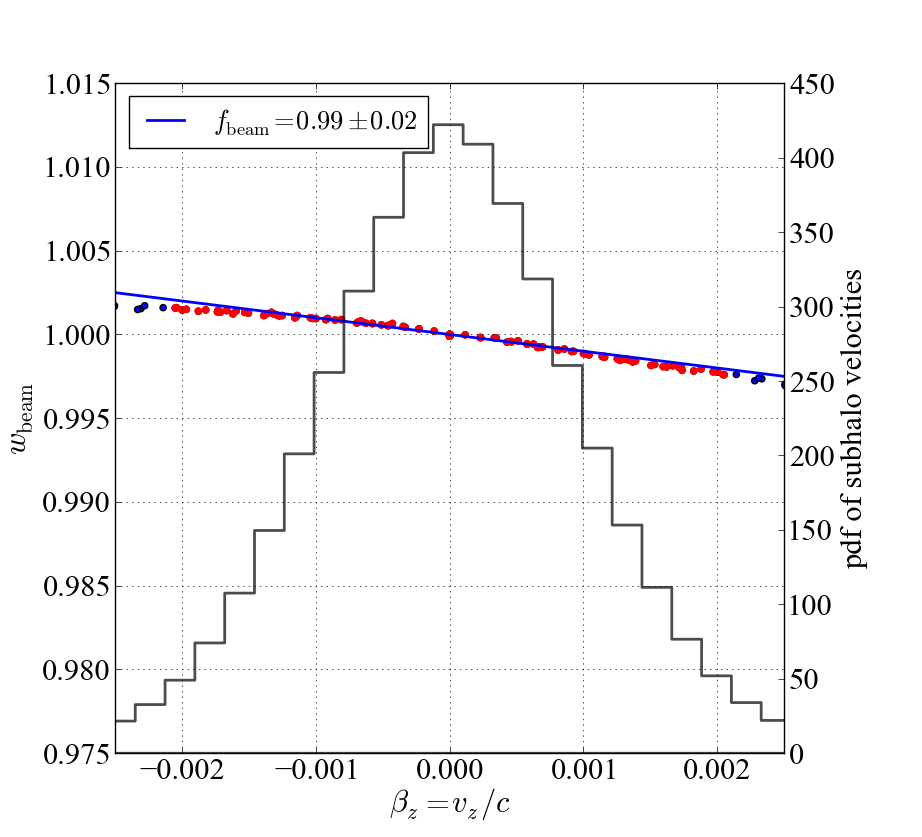
In practice, the magnitude and even the sign of relativistic beaming depends on details of the galaxy spectra as well as their peculiar velocity. When modeling the effect, for simplicity, we introduce a weight for each galaxy in our simulated sample. This weight ($w_{\rm beam}$ below) is given by

$$w_{\rm beam}=1-\beta_{\mathrm{z}}\times f_{\rm beam},$$ (7)

where $f_{\rm beam}$ is a factor which is computed from the spectral characteristics of the galaxy population.

Treating $w_{\rm beam}$ as the probability of including a galaxy in the sample, we can see that Eqn. 7 indicates that we observe all galaxies moving towards us and a fraction of galaxies moving away from us, depending on their line-of-sight velocities. This model is linear in $\beta_{\mathrm{z}}$, and we have found that it behaves robustly when computing the redshift asymmetry using the defined “shell estimator”. We use $w_{\rm beam}$ to weight galaxies before computing their clustering.

The value of $f_{\rm beam}$ depends on the characteristics of the galaxy observational sample we are modeling. A given galaxy catalogue is affected by relativistic beaming when the sample is selected with cuts in colour-magnitude space, because the observed flux of galaxies is altered due to relativistic beaming. K13 made some general assumptions about the spectra of galaxies used in the Wojtak et al. (2011) cluster measurement and assumed the simplest case of a flux-limited sample to derive $f_{\rm beam}=6$. The photometric selection of galaxies in many redshift samples is more complex, however, and to predict the effect of beaming with more accuracy it is necessary to model the specific population of galaxies and selection criteria in detail.

In a companion paper (Alam et al. 2017b) we therefore explore the impact of relativistic beaming on the selection of galaxies in the SDSS/BOSS/CMASS redshift sample. We use the observed spectra as templates to model SRB and define $w_{\rm beam}$ as the ratio of the number of galaxies passing the target selection criteria before and after SRB is applied to their spectra. We find that the spectra and hence values of $f_{\rm beam}$ for each galaxy depend on galaxy stellar mass and redshift. We therefore compute $w_{\rm beam}$ as a function of $\bm{\beta}$, stellar mass and redshift (see Fig. 5 in Alam et al., 2017b). In order to apply the results of this analysis to the simulations in this paper, we compute a representative value of $w_{\rm beam}$ as a function of line-of-sight velocity $\beta_{\mathrm{z}}$ only, by weighting the individual $w_{\rm beam}$ values by the number of galaxies in the corresponding redshift and stellar mass bin in the SDSS/BOSS/CMASS sample.

We find for the purpose of estimating the impact of SRB on clustering asymmetry that Eqn. 7, which is only a linear function of line-of-sight velocity is general enough to adequately model the effect. In Fig. 1 we show the the pdf of subhalo velocities from one of our simulation realizations to illustrate the limited range of peculiar velocities that are relevant. We also plot the $w_{\rm beam}$ values from SDSS/BOSS/CMASS redshift sample (see Alam et al. 2017b), and the linear fit of Eqn. 7 over the range -630 km/s and 630 km/s. The best fitting value of $f_{\mathrm{beam}}$ is 1.0 and we use this value in the rest of this paper.

Figure 1: The effect of relativistic beaming on the probability of including a galaxy in the SDSS/BOSS/CMASS galaxy redshift sample as a function of line-of-sight peculiar velocity. The dots show the probability of including galaxies computed after marginalizing over galaxy stellar mass and redshift using the distribution of data in the observed sample (Alam et al. 2017b). The red dots show data within a velocity range of -630 km/s and 630 km/s, which encompasses 95% of the galaxies in our simulations. The blue line is a fit to the red dots using the functional form of Eqn. 7. The distribution of line of sight galaxy velocities in one of our simulation realizations is shown as a black histogram.

2.5 Luminosity distance perturbation

As was recently reviewed in Kaiser & Hudson (2015), one of the first-order corrections in terms of peculiar velocities is the luminosity distance perturbation. The inferred luminosity of each galaxy, which is inversely proportional to the square of the luminosity distance, is perturbed by the effect of peculiar velocities on the redshift used to calculate that luminosity distance. For simplicity, in our simulations, we assume mass traces light. Under such an assumption, since the flux-distance relation follows an inverse-square law, we can model the mass perturbation in observations using Eqn. 8.

$$M_{\mathrm{obs}}=M\left(\frac{d(z)}{d(z)+\beta_{\text{z}}c/H(z)}\right)^{2},$$ (8)

where $d(z)$ is the comoving distance at redshift $z$ (proportional to the luminosity distance) and $\beta_{\text{z}}c/H(z)$ is the perturbation caused by the peculiar velocity. This pertubation is usually small for SDSS/BOSS/CMASS galaxies at $z=0.57$ (of order a part in one thousand). It can be seen that the lowest order correction is first-order in the peculiar velocity.

A discussion of the first-order velocity contributions can also be found in Eqn. 28 of McDonald (2009), Eqn. 3 of Yoo et al. (2012) and Eqn. 29 of Bonvin et al. (2014). For example, Eqn. 3 of Yoo et al. (2012) gives the luminosity distance contribution as $-5p\delta D_{L}$ where $p$ is the slope of the galaxy luminosity function. However in the discussion in Sec. III of Yoo et al. (2012) it is claimed that first-order relativistic contributions are cancelled, and therefore the Newtonian calculation can fully reproduce Eqn. 3 of that paper. In our paper, we show how first-order and second-order relativistic terms contribute to the signal. The leading first-order relativistic terms are those due to special relativistic beaming and the luminosity distance perturbation. Other first-order relativistic terms are also discussed in Sec. 2.7. The combination of these terms covers the first-order relativistic effects, but in our case as we consider non-linear scales, second-order effects are also important.

2.6 Wide-angle effects

In this paper we have so far assumed the distant observer approximation however this will lead to errors the case of the SDSS/BOSS/CMASS survey. The non-parallel lines-of-sight to galaxies will also induce asymmetries in the 2d cross-correlation functions leading to corrections to the multipoles and shell estimators. From Fig. 12 of Gaztanaga et al. (2015), it can be seen that the wide-angle effects are of the same order of magnitude as the relativistic effects on the $r>20$ Mpc/$h$ scales dealt with in that paper. We compute the correction due to wide-angle effects following Gaztanaga et al. (2015) (see our companion paper Giusarma et al. 2016) for a more detailed treatment and add them to the shell estimator we derived from the distant observer approximation. In Fig. 8 we plot $z^{\rm shell}$, with and without the wide-angle correction. It can be seen that on the small scales which are most important for our current work the wide-angle effect is insignificant.

2.7 Other effects

In the context of galaxy clusters, Cai et al. (2016) recently derived the total redshift of a galaxy relative to a stationary source in the observer’s past light cone. They found that alongside terms that are functions of the peculiar velocity, some additional cross terms eppear (see their Eqn. 12). These cross terms are $-zg_{\mathrm{z}}$ and $Hzv_{\mathrm{z}}/c$, where $-zg_{\mathrm{z}}$ is minus the product of the line-of-sight displacement with the gradient of potential in the line-of-sight direction, and $Hzv_{\mathrm{z}}/c$ is the product of the line-of-sight Hubble velocity with the line-of-sight peculiar velocity. In their simulated cluster-galaxy clustering, on scales $<10$ Mpc/$h$, Cai et al. (2016) find these terms to be as small as the TD effect, while on large scales both terms should vanish because the individual quantities that enter into the cross terms are no longer correlated. We also investigate these two terms in our simulation as follows.

For these two terms, we compute the boosts for each individual subhalo,

$$z_{\mathrm{cross}}=-zg_{\mathrm{z}}+Hzv_{\mathrm{z}}/c.$$ (9)

The pairwise difference is then

$$\begin{split}\delta z_{\mathrm{cross}}&=z_{\mathrm{cross2}}-z_{\mathrm{cross1}}\\ &=z_{1}g_{\mathrm{1,z}}-z_{2}g_{\mathrm{2,z}}+Hz_{2}\beta_{\mathrm{2,z}}/c-Hz_{1}\beta_{\mathrm{1,z}}/c,\end{split}$$ (10)

where $z_{1}$ and $z_{2}$ are line-of-sight distance in real space.

3 Simulation

We have run 8 cosmological $N$-body simulation realizations using the P-Gadget3 code. The cosmological parameters used are summarised in Table 1. In our fiducial runs, we have used $1024^{3}$ particles in a cubic periodic box with side length $1\;\mathrm{Gpc}/h$. The mass per particle is $7.13\times 10^{10}\;M_{\odot}/h$, and the gravitational force softening length is $20\;\mathrm{kpc}/h$. Each simulation starts at $z=159$ and runs till $z=0$. SubFind (Springel et al. 2001b) is used to identify galaxy-sized subhalos. As we mentioned in Sec. 2.1, we take the potential of all stars in a galaxy in a subhalo to be equal to the mean of the potentials of all the particles in the subhalo.

Table 1: Cosmological parameters used in $N$-body simulations

$h$	$\Omega_{\mathrm{baryon}}$	$\Omega_{\mathrm{cdm}}$	$\Omega_{\Lambda}$	Spectral index	$\sigma_{8}$
0.7	0.0462	0.2538	0.7	0.96	0.873285

3.1 Galaxies and large-scale structure

Figure 2: Dark matter distribution with gravitational redshift contours. We show a $10\;\mathrm{Mpc}/h$ thick slice of a cubic box with side length $1\;\mathrm{Gpc}/h$ at $z=0.57$. We also magnify a matter-abundant region $40\times 40\times 10\;\left(\mathrm{Mpc}/h\right)^{3}$ and show its density as well as gravitational redshift contours on the top left panel. The numbers on the contours are in unit of km/s.

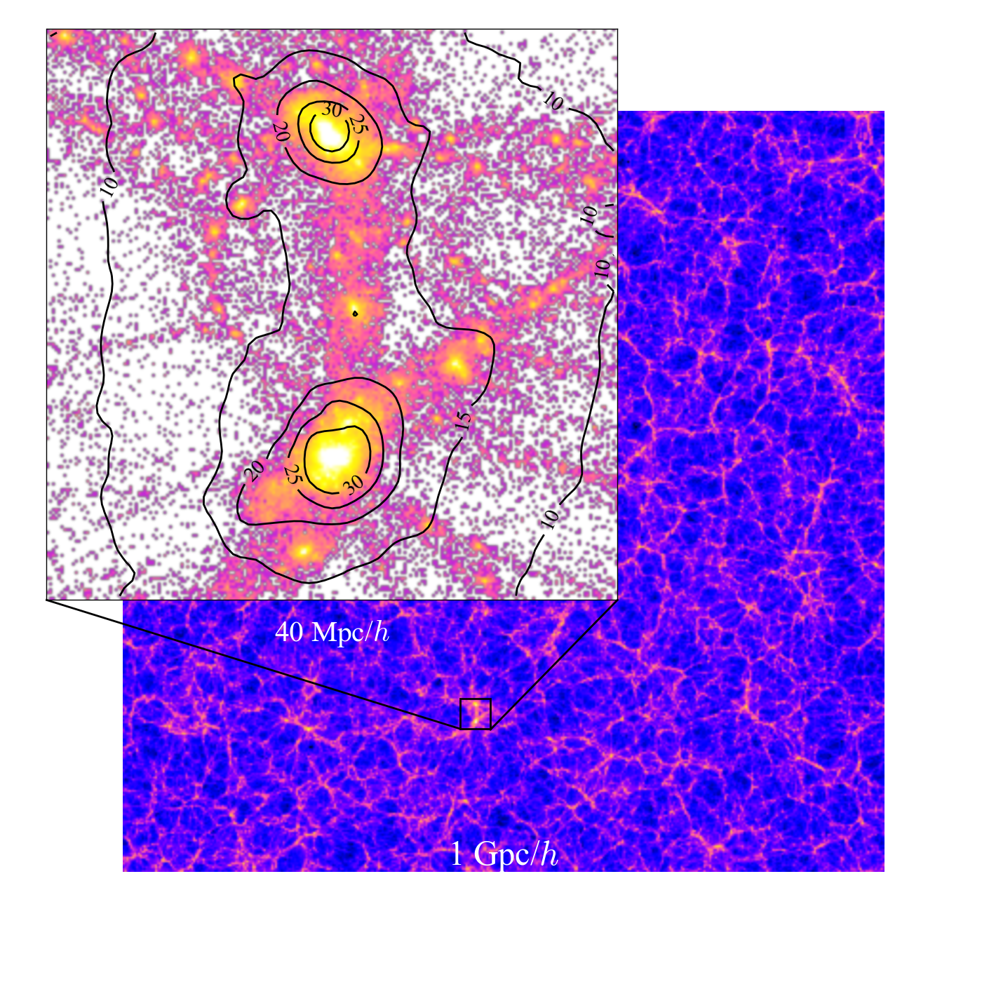
In Fig. 2 we show an illustrative slice through one of the simulation realizations at $z=0.57$. The gravitational potential (redshift) contours are much smoother than the density distribution. The gravitational redshift differences between the centres and edges of the massive (cluster-sized) halos shown in the inset are of order $\sim 10\;\mathrm{km/s}$ as expected. Because the simulations have no model for galaxy formation, we associate galaxies with dark matter subhalos. The more massive galaxies tend to reside inside deeper potential wells while the less massive ones are in shallower potential wells on average. This leads to the difference in $z_{\mathrm{g}}$ when averaged over $g1-g2$ galaxy pairs.

3.2 2d cross-correlation function

We compute the cross-correlation function between two subsamples of galaxies (as in C13 and Bonvin et al. 2014). To create the subsamples, we apply a mass cut to the subhalos in each realization, splitting the subhalo catalogue into two equal number halves. When analyzing observational data, it is usually simplest to apply a luminosity cut, but in our simulations we use mass to divide the samples. In Sec. 4 we explain how we deal with the mapping between mass and luminosity in order to compare to observations.

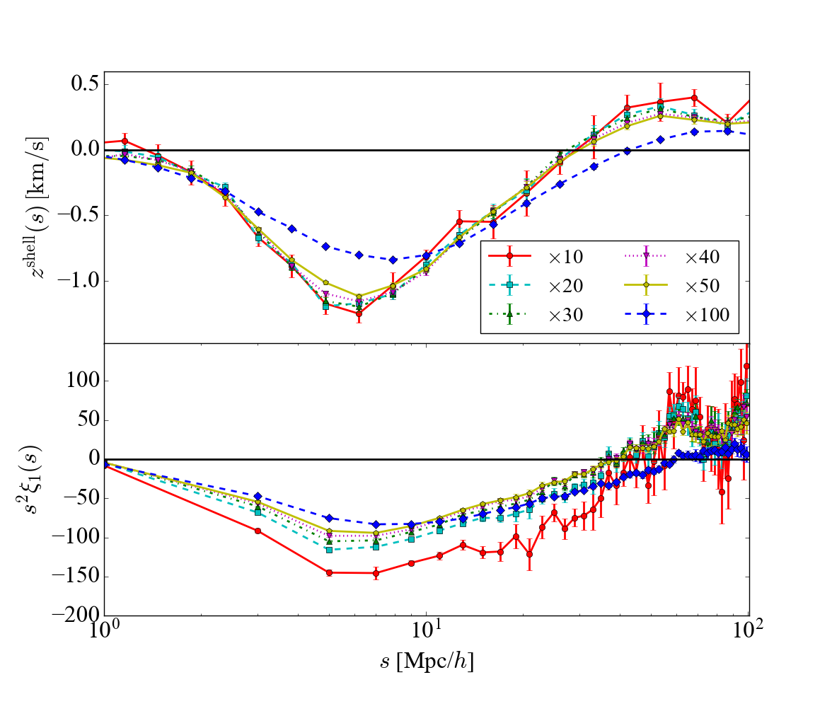
To compute the cross-correlation function in redshift space, which includes the relativistic distortions described in Sec. 2 we first rescale the mass of each galaxy according to LDP, take each galaxy pair, add three components (the gravitational redshift effect, the TD effect and the LC effect), due to the difference in real space $z$, the difference in peculiar velocity and the sum of terms computed from Eqn. 1,  2,  6 and add the wide-angle contribution computed from our companion paper Giusarma et al. (2016). We do not model the relativistic beaming effect directly from redshift differences between galaxy pairs. Instead, we weight each galaxy by the probability given in Eqn. 7. As the relativistic effects are extremely small, we scale up each by a large factor (by multiplying the subhalo velocity that goes into computing each effect by this factor). This enables us to compute the asymmetries in clustering from the simulations with much greater signal to noise, where the statistics are of course appropriately renormalised by the scaling factor after being measured. The choice of factors and tests for convergence are discussed in more detail in Sec. 3.5.

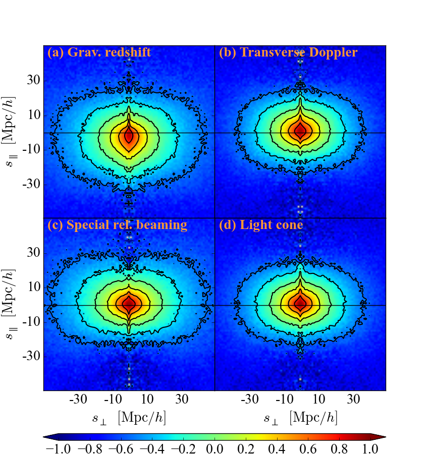
In Fig. 3 we show the cross-correlation function of the $g1$ and $g2$ galaxy samples, as a function of separation parallel and perpendicular to the line of sight. For these illustrative plots, we scale up the relativistic effects by a factor of 250, in order to make them visible. We show the cross-correlation function for each of the four relativistic effects individually. The four effects cause line-of-sight asymmetries with different forms and magnitudes. Comparing the panels we can see that the gravitational redshift and the SRB effect are the dominating two effects. The gravitational redshift effects tends to drag the cross-correlation function bluewards, causing a relative blueshift for the low-mass galaxy ($g2$) with respect to high-mass galaxy ($g1$). This makes sense because low-mass galaxies are more loosely gravitationally bound so that they have smaller gravitational redshifts. The SRB effect causes a “flattening” of the cross-correlation function. The asymmetries due to the SRB, TD and LC effects are difficult to see by eye, but as we show below can be quantified using multipoles and the shell estimator. Note that we do not plot the LDP and the wide-angle effects here. This is because the LDP behaves very similarly to SRB and the wide-angle effects are quite dependent on the bias differences between the two galaxy samples (see Sec. 4).

Figure 3: The 2d 2-pt cross-correlation of the $g1-g2$ galaxy samples for different relativistic effects in the redshift space (plots made using one simulation realization). We exaggerate all the effect by multiplying them with a constant factor of 250. Top left: With Grav. redshifts $\times 250$. Top right: With TD effect $\times 250$. Bottom left: With SRB effect $\times 250$. Bottom right: With LC effect $\times 250$. All four effects are computed at $z=0.57$ with the mass threshold for the $g1$ (high mass) sample being $M_{\mathrm{subhalo}}>10^{13}\;M_{\odot}/h$. In each panel, the colourmap and contours show the distortion of 2-pt cross-correlation function. We have chosen not to plot the LDP and the wide-angle effects here, as LDP is quite similar in effect to SRB (see Fig. 4) and the wide-angle effects are computed independently of the simulations.

3.3 Dipole

We decompose the 2d cross-correlation functions into different moments using Legendre polynomials.

$$\xi_{l}(r)=\frac{2l+1}{2}\int\limits_{-1}^{1}\,\xi(r,\cos\theta)P_{l}(\cos\theta)\,\mathrm{d}\cos\theta,$$ (11)

where $l=0,1,2$ correspond to the monopole, dipole and quadrupole respectively, and $P_{0}(\cos\theta)=1,P_{1}(\cos\theta)=\cos\theta,P_{2}(\cos\theta)=(3\cos^{2}\theta-1)/2$ are the first three Legendre polynomials. The monopole corresponds to the isotropic part of the cross-correlation functions. The quadrupole quantifies the anisotropy in the correlation function in the directions parallel to the line-of-sight and perpendicular to the line-of-sight. The dipole quantifies the asymmetry in the correlation function with respect to positive and negative line-of-sight separations. As we can see from Fig. 3, by carrying out a Legendre decomposition, we could quantify the line-of-sight asymmetries for all four effects using the dipole. The gravitational redshift leads to a relative blueshift for low mass galaxies compared to high mass galaxies, which causes a negative dipole on small scales. On the other hand, on large scales, the correlation function is redshifted along the line-of-sight and more flattened, and we shall see that this leads to a measurable effect of opposite sign. The SRB and LDP effects blueshift the correlation function along the line-of-sight at scales of a few $\mathrm{Mpc}/h$ or less, but redshifts and compresses the correlation function on larger scales. The asymmetries from the TD and LC effects are both smaller, but both lead to a positive dipole (opposite sign to the gravitational redshift) on small scales. To quantify the asymmetries we find that the dipole is not practical in noisy simulations (see Sec.  3.5 for discussion of this point), but instead we use a shell estimator.

3.4 Shell estimator

Another means to make relativistic distortions of clustering measurable is to use the shell estimator which is designed to probe the line-of-sight asymmetry in the cross correlation. C13 designed the estimator to be close in physical meaning to the gravitational redshift profiles measured in galaxy clusters (e.g., by Wojtak et al. 2011). In the shell estimator we bin pairs of subhalos according to their pair separation and average the line-of-sight component of the separation, weighting the pairs by weights from SRB (Eqn. 7) in which the weights fluctuate around 1, effectively computing the redshift displacement of the centroid as a function of pair separation. The mathematical form is Eqn. 12:

$$z^{\text{shell}}(s)=\frac{H\sum\limits_{\alpha\in g1,\beta\in g2}^{|r_{\alpha\beta}-s|<\Delta s}(z_{\alpha}-z_{\beta})w_{\rm beam,\alpha}w_{\rm beam,\beta}}{\sum\limits_{\alpha\in g1,\beta\in g2}^{|r_{\alpha\beta}-s|<\Delta s}w_{\rm beam,\alpha}w_{\rm beam,\beta}},$$ (12)

which is also mentioned in our companion paper (Alam et al. 2017a). This estimator was also used by Gaztanaga et al. (2015) and Alam et al. (2017a). In the measurement with SDSS/BOSS/CMASS samples, the shell estimator is computed from the correlation function and it takes the form of

$$z^{\text{shell}}(s)=\frac{H\int\limits_{0}^{\pi}\text{d}\theta^{\prime}s^{\prime}_{\parallel}\left[1+\xi\left(s^{\prime},\theta^{\prime}\right)\right]}{\int\limits_{0}^{\pi}\text{d}\theta^{\prime}\left[1+\xi\left(s^{\prime},\theta^{\prime}\right)\right]},$$ (13)

where the integral over $\theta^{\prime}$ averages the line-of-sight pair difference $s^{\prime}_{\parallel}$ in each radial bin.

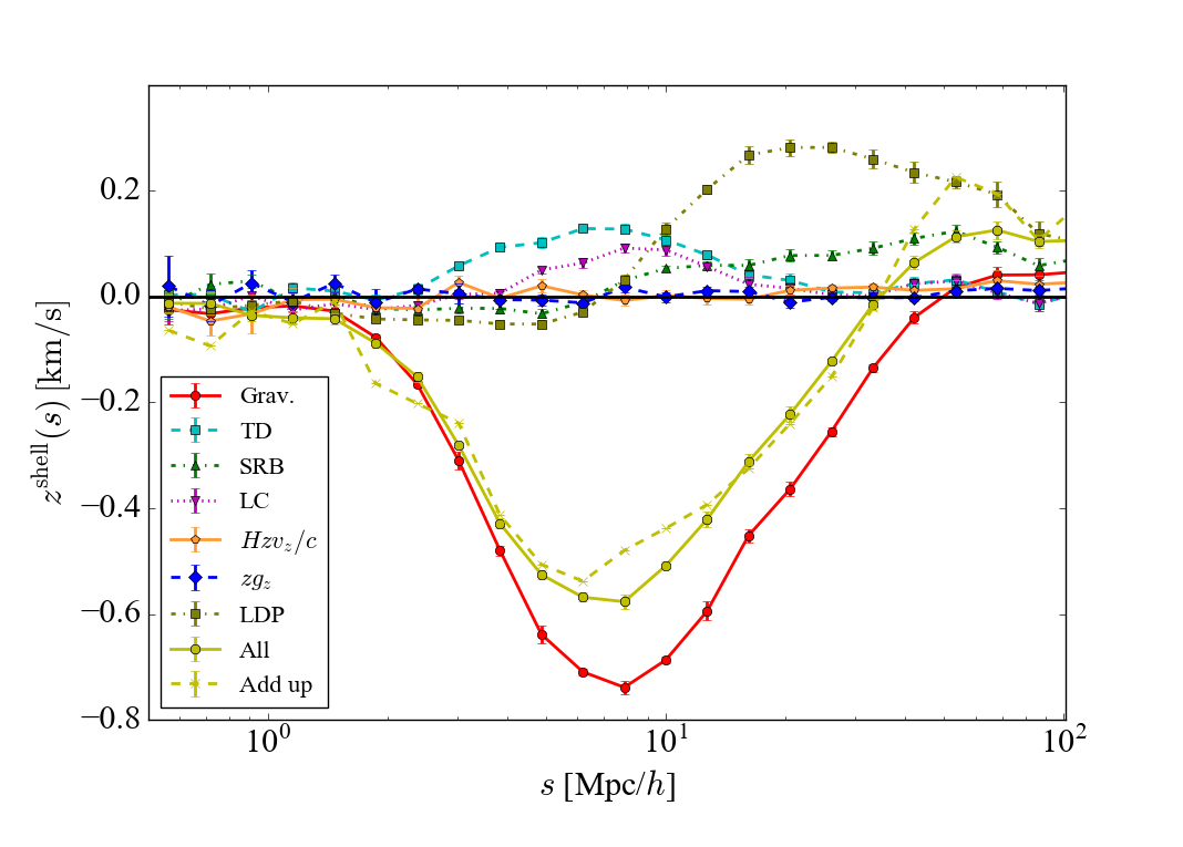
Note that $z^{\text{shell}}$ is zero in real space and $z^{\text{shell}}(s)\rightarrow 0$ as $s\rightarrow 0$ even in redshift space. Fig. 4 shows the contributions to the shell estimator from the four different relativistic effects. Among them, the gravitational redshift effect is the most significant one, causing a relative blueshift for galaxy pairs on small scales, which peaks when $s\sim 8$ Mpc/$h$. The LDP term is the largest in magnitude on scales $s>20$ Mpc/$h$. The SRB effect behaves similarly to the LDP term but with a smaller magnitude. Also, the LDP and SRB effects do change sign, at $s\sim 8$ Mpc/$h$ – there is a relative blueshift at small scales and a relative redshift at large scales. Although there is a quite complex interaction between galaxy spectra and SRB (see Alam et al. 2017b), one can approximately explain this pattern as being due to infall on large scales and virialised motions on small scales. The mean relative line-of-sight peculiar velocity of pairs of galaxies with given redshift separation $s$ will therefore change sign as we move between these two regimes, and this leads to a change of sign in $z^{\text{shell}}$.

The next effects in order of significance seen in Fig. 4 are the TD and the LC effects. They result in a relative redshift at all scales since high mass galaxies move more slowly on average than the lower mass member of a pair. The least significant effects are the cross terms $Hzv_{z}/c$, $zg_{z}$ discussed in Cai et al. (2016). Our $g1-g2$ galaxy cross-correlation almost shows no sign of these two effects. This is expected as both subsets $g1$ and $g2$ contain equal numbers of galaxies, which leads to small correlations in $z$, $v_{z}$ and $g_{z}$ when averaging over populations of relatively similar objects. These effects are even smaller that for the cluster-galaxy cross-correlation case simulated by Cai et al. (2016), where they were also not significant compared to the gravitational redshift.

We also show in Fig. 4 the combined effect (“all”) which we obtain by adding each of five effects (the gravitational redshift, TD, SRB, LC and LDP) to the subhalo positions in redshift space. The curve labelled “add up” is the sum of these individual five effect curves (computed by measuring $z^{\text{shell}}$ from galaxy catalogues with only one relativistic effect included at a time). The two curves (“all” and “add up”) agree quite well, showing that the effects can be added linearly, even on these relatively small scales. However, we find taking account of two cross terms only adds noise to the overall signal. Therefore we only consider the five effects mentioned while excluding those two cross terms. The amplitude of $z^{\text{shell}}$ while including all the effects is dominated by the gravitational redshift effect on small scales and the LDP effect on large scales ($s>30$ Mpc/$h$).

Figure 4: The shell estimator Eqn. 13, of clustering asymmetries computed from the cross-correlation function of $g1-g2$ galaxy samples. We show the different relativistic effects individually: the gravitational redshift, TD, SRB, LC, $Hzv_{z}/c$, $zg_{z}$ and LDP. The curves are the average of results from 8 realizations at $z=0.57$ with masscut $3\times 10^{13}\,M_{\odot}/h$. The error bars show the errors on the mean. The solid yellow line shows $z^{\text{shell}}$ for the five significant effects (the gravitational redshift, TD, SRB, LC, LDP) included at once and the dashed yellow line is the sum of the curves for these five effects. Here a boost factor 100 is applied. How the boost factor is chosen is discussed in Sec. 3.5

.

3.5 Increasing the signal to noise ratio of the simulation predictions

As we mentioned in Sec. 3.3 and Sec. 3.4, both the dipole and the shell estimator are capable of quantifying the signal due to relativistic effects (the antisymmetric part of the cross-correlation function could also be used- see e.g., Iršič et al. 2016). We choose the shell estimator for three reasons. First, the shell estimator shows the signal in km/s units, which serves as a direct way to express line-of-sight redshift (velocity) distortions. Second, we have seen in Sec. 2 that the asymmetry signal on small scales is dominated by the gravitational redshift, and this has already been quantified using the very similar gravitational redshift profile in several published works on galaxy clusters.

A third and more practical reason to prefer shell estimator has to do with the limitations of our simulations. Since our simulations are only 1 (Gpc/$h$)³ in volume the signal we measure will be quite noisy due to the intrinsically asymmetric shapes of large-scale structures not being fully averaged out in the cross-correlation function. In order to reduce the relative effect of noise we boost each of the relativistic effects by multiplying the input peculiar velocity of each halo by multiplication factor, and then account for the multiplication factor in the final measurement. Ideally, using different multiplication factors should only change the noise characteristics of the signal without affecting its amplitude and shape. In practice, this is something which must be explored with a convergence test, as described below.

We have performed the measurement of the shell estimator and dipole moment for a series of different multiplication factors, and the results are shown in Fig. 5. The top panel shows the shell estimator and bottom panel shows the dipole moment. The error bars are obtained from the errors on the mean of 8 simulation realization. We observe from the top panel that the prediction for the shell estimator is largely independent of the factor used but the dipole moment is highly sensitive to the factor. This behavior is likely due to the fact that the definition of the shell estimator includes a normalization in the denominator which balances the effect of the boost factor, something which is not the case for the computation of the dipole moment. To be specific, both the numerator and denominator in either Eqn. 12 or Eqn 13 will fluctuate somewhat coherently and mostly cancel or reduce the non-linear effect when boosting while the dipole moment will not. We do find that shell estimator has some weak dependence on the multiplication factor, and that this becomes most noticeable when the boost factor is increased to 100 or more. When the boost factor is this large the relativistic effects change the line-of-sight separation by significantly more than a bin size. This leads to a shifting of the minimum to right and a dilution of the amplitude of the signal. We therefore decide to use the boost factor with good signal to noise while making sure that we are in a regime where the shell estimator is independent of the boost factor. Examining the $z^{\rm shell}$ signal in Fig. 5 close to the minimum, we can see that a boost factor of 50 leads to a statistical error bar of $\sim 5\%$, and the systematic error from the behaviour of the convergence at low factors is similar or less than this. We therefore choose a boost factor of 50 in this paper to make our predictions for $z^{\rm shell}$.

Figure 5: The shell estimator and the dipole moment for different multiplication factors. The $x$-axis represents the pair separation in the log space. The colour and style schemes are the same for both panels. The circles with the solid line (red), the squares with the dashed line (cyan), the triangles with the dash- dotted line (green), the upside down triangles with the dotted line (magenta), the pentagons with the solid line (yellow) and the diamonds with the dashed line show the two estimators computed using multiplication factors of 10, 20, 30, 40, 50, and 100 respectively. In each case, the peculiar velocities entering in to the calculation of relativistic effects were multiplied by this factor, and then the measure statistic ($z^{\rm shell}$ or dipole) was divided by the same factor before plotting (see text). The error bars are the errors on the mean of 8 simulation realizations. Note that the shell estimator has a much weaker dependence since the normalization saturates such dependence.

4 Simulating an observed sample of galaxies

4.1 Galaxy bias

We can study the distribution of galaxies from both observations and simulations since galaxies are used as tracers of the matter in the Universe. Galaxies are “biased” tracers in the sense that the physics of galaxy formation can influence the relationship between galaxies and matter. The simplest parametrization of this relationship, galaxy bias measures the difference between the spatial distribution of galaxies and the underlying dark matter density field. It is defined as

$$\delta_{\mathrm{g}}=f(\delta_{\mathrm{m}}),$$ (14)

here $\delta_{\mathrm{g}}=\rho_{\mathrm{g}}/\bar{\rho_{\mathrm{g}}}-1$ represents the mean overdensity of galaxies and similarly $\delta_{\mathrm{m}}$ represents the mean overdensity of matter. The function $f(\delta_{\mathrm{m}})$ depends on both scale and galaxy evolution. On large scales, the galaxy bias is linear and takes the following form

$$b=\frac{\delta_{\mathrm{g}}}{\delta_{\mathrm{m}}}=\sqrt{\frac{\xi_{\mathrm{g}}}{\xi_{\mathrm{m}}}},$$ (15)

where $\xi_{\mathrm{g}}$ and $\xi_{\mathrm{m}}$ are the 2-pt cross-correlation functions of galaxy-matter and matter-matter respectively.

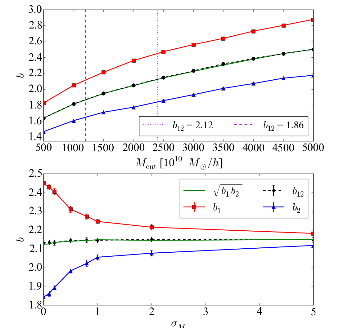
Our primary application of the work in this paper is a prediction for the clustering asymmetry measured from the SDSS/BOSS/CMASS redshift sample in our companion paper (Alam et al. 2017a). As a result, we would like our simulated galaxy catalogue to have the same galaxy bias properties as the observed sample. In order to achieve this, we vary two parameters, the lower limit on the subhalo mass threshold to be allowed into the sample, and a subhalo mass error $\sigma$. The latter is a random variable (normally distributed in $\log(M)$) which we add to the subhalo masses in order to model the scatter between the observed quantity (e.g., luminosity) and mass. The subhalo mass after adding the scatter is

$$\log_{10}M_{\rm obs,i}=\log_{10}M_{i}+\sigma_{i},$$ (16)

where $\sigma_{i}$ is a normally distributed random variable with zero mean and standard deviation $\sigma$, and $M_{i}$ is the actual mass of subhalo $M_{i}$. This mass error is adjusted by tuning the spread of the Gaussian $\sigma$.

As before, we split our subhalo samples into two halves, but this time using $M_{\rm obs,i}$. We compute the bias of the two samples with respect to the dark matter by averaging Eqn. 15 over scales $r=20-50$ Mpc/$h$. We compute results at a simulation output redshift $z=0.57$ which is the mean redshift of the CMASS sample (Alam et al. 2017a). In the top panel of Fig. 6 we show the effect of a changing mass threshold on the bias $b_{1}$ measured from the high mass half, $b_{2}$ (low mass half) and $b_{12}$, the entire sample. We also show $\sqrt{b_{1}b_{2}}$, which is consistent with $b_{12}$, as expected. A higher mass cut eliminates more low bias galaxies and thus increases the bias overall. The lower mass threshold of $M=1.2\times 10^{13}\,M_{\odot}/h$ reproduces the $b_{12}=1.86$ found by Gaztanaga et al. (2015) for the CMASS sample. The higher mass threshold $M=2.4\times 10^{13}\,M_{\odot}/h$ reproduces the $b_{12}=2.12$ measured by Alam et al. (2017a) for the full CMASS sample (his Fig. 5). In the top panel of Fig. 6, no extra scatter was added to the masses (i.e. $\sigma=0$ in Eqn. 16). The difference between $b_{1}$ and $b_{2}$ is therefore maximised.

Bonvin et al. (2014) and Gaztanaga et al. (2015), showed that in linear theory the asymmetry of cross-correlation functions (quantified by the dipole, or $z^{\text{shell}}$) is proportional to the bias difference $b_{1}-b_{2}$. In order to match the bias difference of an observed sample, we vary $\sigma$. In the bottom panel of Fig. 6, we show how $\sigma$ affects the values of $b_{1}$ and $b_{2}$. When $\sigma$ is large, the larger scatter between $M$ and $M_{\rm obs}$ means that the two halves overlap much more and consequently have smaller $b_{1}-b_{2}$.

Figure 6: Biases of two galaxy subsets at $z=0.57$ as a function of the subhalo mass cut and spread. In both subplots, $b_{1}$, $b_{2}$, $b_{12}$ are the bias factors of the high mass subhalo subset, the low mass subhalo subset and two subsets respectively. The solid green curves are the geometric mean of $b_{1}$ and $b_{2}$. The dashed and dotted magenta line on the top panel indicate the mass cut where $b_{12}=1.86$ and $b_{12}=2.12$ respectively.

5 The influence of structure on galaxy and halo scales

Although there is large-scale structure in the gravitational potential (e.g., Fig. 2) which contributes to the asymmetry of clustering signal, the light from galaxies must also exit the potential well of the subhalo, and this must also be accounted for. We find that the signal (e.g., from $z^{\text{shell}}$) is in fact very sensitive to the gravitational potential on small scales, and we explore this here.

5.1 Gravitational potentials of subhalos

The simulated data includes gravitational potentials for each particle in each subhalo. One therefore needs to decide given this information what the inferred gravitational potential of a galaxy residing in the subhalo would be. In our previous results in this paper we have taken the mean potential of all particles belonging to a subhalo as the potential of the galaxy. As luminous galaxies will tend to lie in the densest part of a subhalo, and therefore trace these regions, then averaging over the subhalo instead will clearly suppress the signal of the gravitational redshift effect. Another choice is to use the potential of the most bound particle inside each subhalo. As can be seen from the contours of the top left panel in Fig. 2, the bound particles around the centre have significantly higher gravitational redshifts.

Additional sources of difference between the potentials of galaxies and subhalos could be the influence of galaxy formation physics (gas cooling, star formation), as well as structure on the scales of galaxies which we do not resolve in our simulation. We explore this in more detail with hydrodynamic simulations in future work (Zhu et al. 2016, in preparation), but for now we can assess the potential differences using an analytic galaxy model. We use the result for the gravitational redshift profile for a galaxy with the approximation due to Cappi (1995) (his Eqn. 7):

$$\begin{split}V(R)&\simeq\frac{GM}{cR_{0}}\left[1+\ln\left(\frac{R_{0}}{R}\right)\right]\\ &\simeq 10^{-5}\sigma_{v}^{2}\left[1+\ln\left(\frac{R_{0}}{R}\right)\right],\end{split}$$ (17)

where $R_{0}=3R_{\mathrm{e}}$, $R_{\mathrm{e}}$ is the half-mass radius and $\sigma_{v}$ is the galaxy velocity dispersion which is correlated with galaxy mass. As is pointed out by Cappi (1995), this is a good approximation to the projected gravitational potential profile within the range $0.05R_{\mathrm{e}}<R<3R_{\mathrm{e}}$.

So far in our analysis of the simulations we have been using the distribution of dark matter particles. We expect the stellar mass to be more concentrated, however, so that the effective radius of stars will be different to the dark matter. In order to take this into account, we use results from hydrodynamical simulations to estimate how the stars contribute to the potentials via the analytic potential profile. We randomly choose 20 subhalos with $M_{\mathrm{sub}}>3\times 10^{13}M_{\odot}/h$ in the MBII hydrodynamic simulations (Khandai et al. 2015; Zhu et al. 2016) and compute the half-mass radius of the star $R_{\mathrm{e,star}}$ and darkmatter $R_{\mathrm{e,dm}}$ particles respectively. We use these results to estimate the increment of the redshift of galaxies from star particles on a galaxy by galaxy basis as follows:

$$\begin{split}z_{\mathrm{galaxy}}&=V(R_{\mathrm{e,star}})-V(R_{\mathrm{e,dm}})\\ &\simeq 10^{-5}\sigma_{v}^{2}\ln\left(\frac{R_{\mathrm{e,dm}}}{R_{\mathrm{e,star}}}\right),\end{split}$$ (18)

where the galaxy velocity dispersions ($\sigma_{v}$) are taken from our $N$-body subhalo catalogues.

Figure 7: The clustering asymmetry $z^{\text{shell}}$ measured from simulations using different prescriptions for the galaxy potential on subhalo scales. Only gravitational redshift effects are included. The circles with solid lines (red) show the effect of taking the galaxy potential to be the mean potential of all the subhalo particles. The squares with the dashed line (green) show the galaxy potential as the potential of the most bound subhalo particle. The triangles with the dash dotted line (blue) and the upside down triangles with the dotted line (cyan) include the effect of internal galaxy structure using Eqn. 17. The error bars are the errors on the mean of 8 simulation realizations.

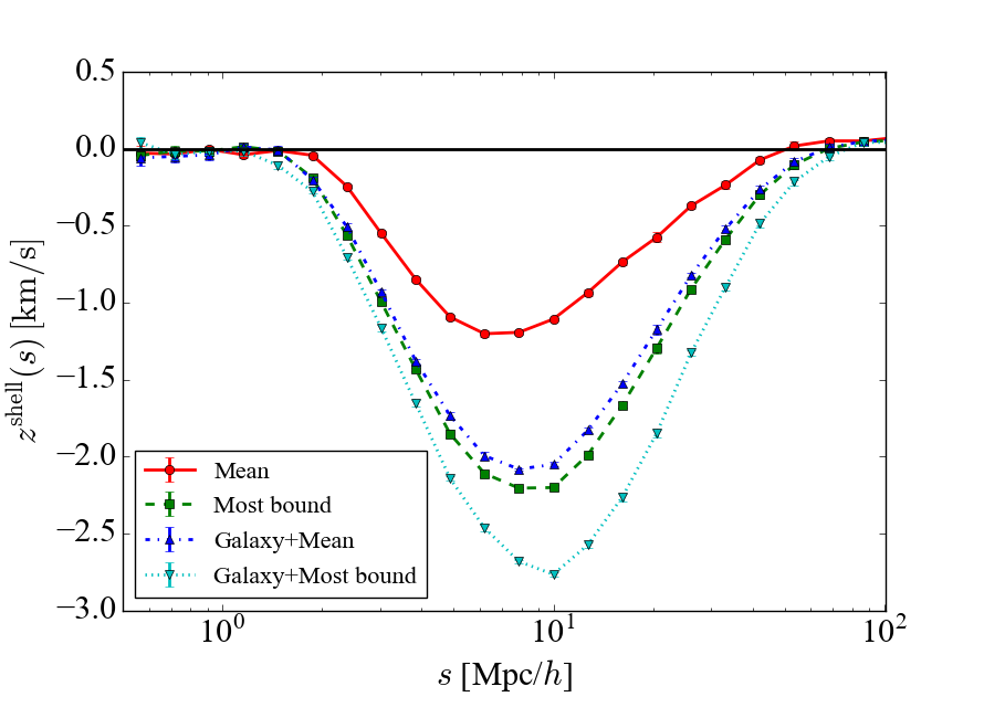
In Fig. 7 we show how the different means of modelling the galaxy potential from the subhalos affect the clustering asymmetry due to $z^{\text{shell}}$. We only include the effect of gravitational redshifts here, although a full accounting should also include relativistic effects due to beaming and transverse Doppler shifts of stars for example. We can see by adding galaxy structure information onto the fiducial simulation (which only includes large-scale structure), the amplitude of $z^{\text{shell}}$ can increase dramatically. In fact for the example plotted in Fig. 7, most of the asymmetry is due to structure on galactic scales, even when measured using the cross-correlation function on 10 Mpc/$h$ scales. The fact that there is this dramatic difference underscores the need for a better understanding of the small-scale contributors to relativistic clustering distortions. The largest uncertainty in our current predictions is therefore due to this small-scale structure, and this should be borne in mind when comparing to observations. We note that although the mean and most bound potentials have a significantly different amplitude on their own, when including a galaxy component the difference between mean and most bound potential becomes small.

Figure 8: The clustering asymmetry $z^{\mathrm{shell}}$ from simulations including all the components discussed above. The dashed blue line represents the wide-angle effects computed in Giusarma et al. (2016). The solid blue line includes the five effects discussed above (computed using a boost factor of 50) but without the wide-angle effects. The solid red line adds the wide-angle effects on top of the solid blue line, and this is used as the model fit in our companion paper Alam et al. (2017a). The error bars are the errors on the mean of 8 simulation realizations.

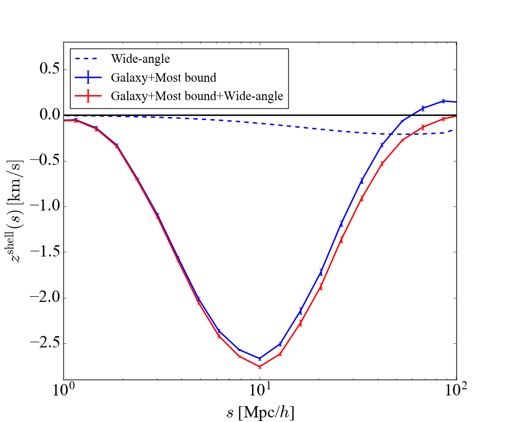
We have chosen the multiplication factor appropriate for making low noise predictions of the relativistic asymmetry ( see Sec. 3.5 for discussion of this factor). In Figure Fig. 8 we show the component due to wide-angle effects as well as the associated $z^{\text{shell}}$ results from the simulation, which we use as our model fit in the measurement of clustering statistics in the BOSS/CMASS galaxy sample Alam et al. (2017a). We see that the wide-angle effects lead to a $\sim-0.2$ km/s offset in this case, which is small compared with overall amplitude of Gravitational redshift effects.

5.2 Resolution test

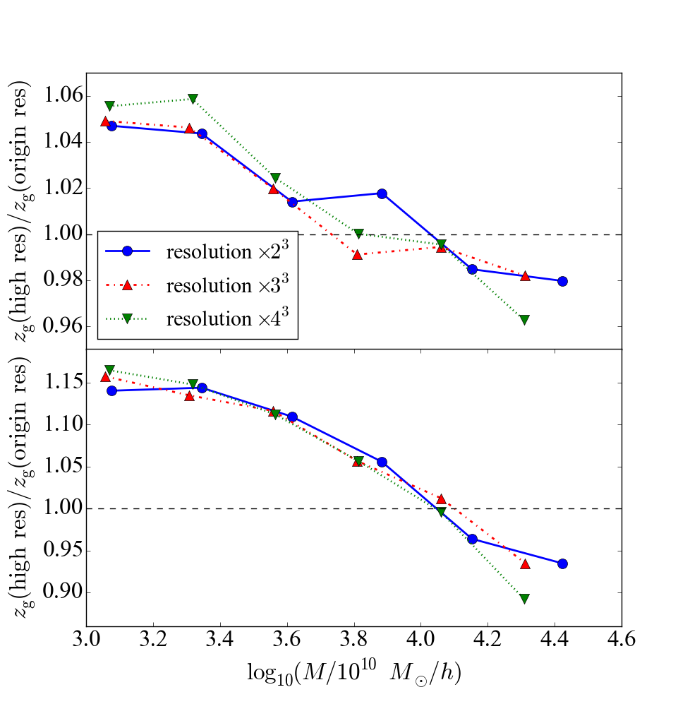
The resolution of the simulation can affect the shell estimator as well. If the simulation cannot resolve the subhalos very well, the signal will also be suppressed. We construct a resolution test for only one realization in a smaller box with side length 125 Mpc/$h$ by running new simulations of the same cosmological model, but with higher mass and spatial resolution, doubling, tripling and quadrupling the number of particles per Mpc/$h$ along each dimension compared to our fiducial simulations. The numbers of particles along each dimensions are 128, 256, 384, 512 so that the resolutions are “resolution”, “resolution$\times 2^{3}$”, “resolution$\times 3^{3}$” and “resolution$\times 4^{3}$” accordingly. We change the mass and force resolution together and thus the softening length becomes 2.5 kpc/$h$.

We run the simulations using the same initial random phases and the same box sizes, so that we are able to match subhalos in the different resolution runs according to their positions. We then compare the $z_{\mathrm{g}}$ (gravitational redshifts) of the same subhalos between different resolutions. The results for the mean ratio of $z_{\mathrm{g}}$ as a function of subhalo mass for the different runs. are shown in Fig. 9. The top panel was computed using the mean potential of subhalo particles and the bottom panel from the most bound subhalo. As expected, the difference due to resolution for the latter is greater. We can also see that the results have effectively converged with a resolution which is twice as good as our fiducial resolution. The maximum differences in $z_{\mathrm{g}}$ between our fiducial simulation and the converged run are between 5% and 15%. Given the much larger uncertainties in structure on galactic scales discussed above, this is acceptable.

Figure 9: Resolution test of the subhalo potentials. Each panel shows the mean value of the ratio of $z_{\mathrm{g}}$, the gravitational redshift measured from a set of halos in higher resolution simulations divided by the results for the same halos (see text for matching) in a simulation with our fiducial resolution. The top panel associates the galaxy potential with the mean potential of all particles in the subhalo. In the bottom panel we show results when the galaxy potential is associated with the potential of the most bound subhalo particle.

6 Summary and discussion

6.1 Summary

Using $N$-body simulations, we have modeled different relativistic effects which cause small asymmetries in the clustering of galaxies. These effects, such as the gravitational redshift have previously been observed in galaxy clusters (e.g., Wojtak et al. 2011). We have extended the study of other effects such as the transverse Doppler effect and relativistic beaming modeled in clusters by Zhao et al. (2013) and K13 to the case of large scale structure. We have focussed on non-linear scales $\sim 10$ Mpc/$h$ and below, where perturbation theory results (e.g., Yoo et al. 2009; Yoo et al. 2012; Bonvin et al. 2014) are less likely to be accurate, and followed the quasi-Newtonian approach taken by C13 for gravitational redshifts. We have made predictions for the distortions in the galaxy cross-correlation function of galaxies with different mass and bias, and quantified the line-of-sight asymmetries. Our conclusions are as follows:

1. The centroid of the galaxy high mass versus low mass cross-correlation function is shifted in the line-of-sight direction by a maximum of around 2-3 km/s on scales $\sim$ 10 Mpc/$h$. This is smaller than the redshift profile shift seen in galaxy clusters (e.g., Wojtak et al. 2011) by around an order of magnitude.

2. All five relativistic effects we include (the gravitational redshift effect, the TD, LC, SRB and LDP effects) lead to asymmetries in the cross-correlation functions, but with differences in magnitude, sign and variation with scale. The LC and TD effects cause a positive shift ($z^{\rm shell}$ positive) on scales $s\sim 10$ Mpc/$h$. The asymmetry signal is however dominated by the gravitational redshift effect on scales $s\sim 10$ Mpc/$h$, and has opposite sign. At larger scales the effect of luminosity distance perturbations and the effect of special relativistic beaming on galaxy selection becomes more important, which again leads to an overall positive shift in $z^{\rm shell}$. Finally, wide-angle effects are added, which depend on the galaxy bias differences. These lead to an overall small blueshift or redshift offset to the signal on large-scales.

3. We compare two estimators of clustering asymmetry– the shell estimator and the dipole. We find that the shell estimator is mostly independent of the multiplication factor used in simulations to increase the signal to noise, while the dipole moment is not. Because of this we focus on the shell estimator, and adjust the multiplication factor so that the statistical and systematic errors from our simulation predictions are approximately equal (and below 5%).

4. We find that approximately half or more of the observable asymmetry signal is likely caused by potential gradients from structure on galaxy scales instead of the large-scale information.

6.2 Discussion

Some of the uncertainties in our predictions, can be traced to small-scale physics and the uncertainties in the subhalo gravitational potentials. For example, we have experimented using different ways to map the potentials of particles in subhalos to the potentials of galaxies – the mean and the potential of the most bound particle, finding approximately twice the signal using the potential of the most bound particle. We have also investigated the influence of structure on galactic scales, adding the contribution of a galaxy potential profile, and find that this can strongly affect the shell estimator of asymmetry. The galaxy structure can therefore be thought to be the main uncertainty, (which we have seen can vary the signal by a factor of two). It will therefore require further work before we are able to make predictions for redshift asymmetries expected in the LCDM model at the few tens of percent accuracy expected to be relevant for testing modified gravity theories (e.g., Wojtak et al. 2011; Gronke et al. 2014). Not only dark matter but also baryons will contribute to the galaxy structure (for example, through the processes of cooling and feedback). In this paper, we have used purely $N$-body simulations but we explore hydrodynamic effects using hydrodynamic simulations in a companion paper (Zhu et al. 2016, in preparation).

On the observational side, there are many promising current and future datasets which can be used to measure these relativistic clustering asymmetries. We have used our work on simulations to develop a model relevant to the CMASS galaxy sample from the SDSS BOSS redshift survey. Our observational measurements and comparison with this model are presented in a companion paper (Alam et al. 2017a). In the future, surveys such as eBOSS (Dawson et al. 2016) and DESI (Levi et al. 2013) will be used to push the measurement of gravitational redshift and other asymmetries of clustering forward. On small scales, the potential profiles inside galaxies can in principle be measured by stacking integral field spectra of large numbers of galaxies. This could allow tests of relativistic effects including gravitational redshifts and beaming of stars on galactic scales, which we have shown our knowledge is uncertain. The SDSS MaNGA (Bundy et al. 2015) survey of large numbers of galaxies will be a useful dataset in this regard and we have started investigating this area.

On the theory side, although we have used $N$-body simulations here, it should be possible to develop a halo model (Cooray & Sheth 2002) for all relativistic clustering effects (TD, LC, SRB and LDP). This would be along the lines of what was done by C13, for example to make predictions for the gravitational redshift. Such a semi-numerical model might enable a range of models to be covered more rapidly, although testing with $N$-body simulations will be needed. Alternative theories to GR (modified gravity, Clifton et al. 2012) have taken on more prominence during the past decade. Modified gravity models may make different predictions for the clustering asymmetries and they could also be simulated.

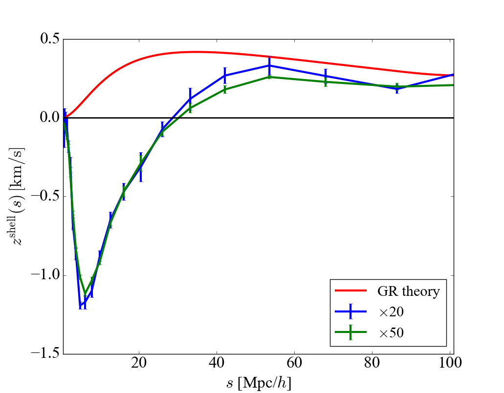
It is useful to compare our results to the GR perturbation theory predictions in the literature (e.g., Bonvin et al. (2014)), as we should expect a level of agreement on linear scales. We have done this in Fig. 10, where we use a linear $x$-axis to better show the range of scales where predictions can be compared. To compute the linear pertubation theory curves, we have followed the methodology of Giusarma et al. (2016) (based on Bonvin et al. (2014)), applying the relevant galaxy biases for our samples. We can see that large scales ($>30$ Mpc/$h$, our the shell estimator from the simulations is quite close to that from linear perturbation theory, and has the correct sign. They are not expected to be identical because proper modelling of the special relativistic beaming effect requires using the colour-magnitude selection appropriate for BOSS galaxies, which we have done in the simulation, but which is not accounted for explicitly in the linear perturbation theory result.

Figure 10: Comparison between our shell estimator with different boost factors (blue, green) and the linear perturbation theory (red). The biases ($b_{1}=2.57$, $b_{2}=1.91$) are chosen at $M_{\mathrm{cut}}=3\times 10^{10}\,M_{\odot}/h$ and $\sigma_{M}=0$. Though they disagree on small scales but converge at sufficient large scales.

In this paper we have used a quasi-Newtonian approach, with $N$-body simulations to model non-linear effects. The reasoning behind this is that the largest uncertainties are due to these non-linearities (including for example structure on galactic scales), and the signal to noise of future measurements from large-scale structure and current measurements from clusters is dominated by non-linear scales. The fully General Relativistic perturbation theory (PT) approach has been used successfully by e.g., Yoo et al. (2009), Bonvin et al. (2014) to make predictions for relativistic clustering on large, linear scales. Comparison of the two approaches is needed to find areas of overlap and explore the consistency of predictions (see for example, Giusarma et al. 2016, in preparation).

References

- Alam et al. (2016) Alam S., Ho S., Silvestri A., 2016, MNRAS, 456, 3743
- Alam et al. (2017a) Alam S., Zhu H., Croft R. A. C., Ho S., Giusarma E., Schneider D. P., 2017a, Monthly Notices of the Royal Astronomical Society, 470, 2822
- Alam et al. (2017b) Alam S., Croft R. A. C., Ho S., Zhu H., Giusarma E., 2017b, Monthly Notices of the Royal Astronomical Society, 471, 2077
- Blake et al. (2013) Blake C., et al., 2013, MNRAS, 436, 3089
- Bonvin et al. (2014) Bonvin C., Hui L., Gaztañaga E., 2014, Phys. Rev. D, 89, 083535
- Bundy et al. (2015) Bundy K., et al., 2015, ApJ, 798, 7
- Cai et al. (2016) Cai Y.-C., Kaiser N., Cole S., Frenk C., 2016, preprint, (arXiv:1609.04864)
- Cappi (1995) Cappi A., 1995, A&A, 301, 6
- Clifton et al. (2012) Clifton T., Ferreira P. G., Padilla A., Skordis C., 2012, Phys. Rep., 513, 1
- Colless et al. (2003) Colless M., et al., 2003, ArXiv Astrophysics e-prints,
- Cooray & Sheth (2002) Cooray A., Sheth R., 2002, Phys. Rep., 372, 1
- Croft (2013) Croft R. A. C., 2013, MNRAS, 434, 3008
- Davis & Peebles (1983) Davis M., Peebles P. J. E., 1983, ApJ, 267, 465
- Dawson et al. (2016) Dawson K. S., et al., 2016, AJ, 151, 44
- Domínguez Romero et al. (2012) Domínguez Romero M. J. d. L., García Lambas D., Muriel H., 2012, MNRAS, 427, L6
- Durrer (1994) Durrer R., 1994, Fundamentals Cosmic Phys., 15, 209
- Eisenstein et al. (2011) Eisenstein D. J., et al., 2011, AJ, 142, 72
- Gaztanaga et al. (2015) Gaztanaga E., Bonvin C., Hui L., 2015, preprint, (arXiv:1512.03918)
- Giusarma et al. (2016) Giusarma E., Alam S., Zhu H., Croft R. A. C., Ho S., 2016, xxx, pp xx–xx
- Greenstein et al. (1971) Greenstein J. L., Oke J. B., Shipman H. L., 1971, ApJ, 169, 563
- Gronke et al. (2014) Gronke M. B., Llinares C., Mota D. F., 2014, A&A, 562, A9
- Hernquist (1990) Hernquist L., 1990, ApJ, 356, 359
- Iršič et al. (2016) Iršič V., Di Dio E., Viel M., 2016, J. Cosmology Astropart. Phys., 2, 051
- Jimeno et al. (2015) Jimeno P., Broadhurst T., Coupon J., Umetsu K., Lazkoz R., 2015, MNRAS, 448, 1999
- Kaiser (1987) Kaiser N., 1987, MNRAS, 227, 1
- Kaiser (2013) Kaiser N., 2013, MNRAS, 435, 1278
- Kaiser & Hudson (2015) Kaiser N., Hudson M. J., 2015, MNRAS, 450, 883
- Khandai et al. (2011) Khandai N., Sethi S. K., Di Matteo T., Croft R. A. C., Springel V., Jana A., Gardner J. P., 2011, MNRAS, 415, 2580
- Khandai et al. (2015) Khandai N., Di Matteo T., Croft R., Wilkins S., Feng Y., Tucker E., DeGraf C., Liu M.-S., 2015, MNRAS, 450, 1349
- Kim & Croft (2004) Kim Y.-R., Croft R. A. C., 2004, ApJ, 607, 164
- Levi et al. (2013) Levi M., et al., 2013, preprint, (arXiv:1308.0847)
- Liske et al. (2015) Liske J., et al., 2015, MNRAS, 452, 2087
- Lopresto et al. (1991) Lopresto J. C., Schrader C., Pierce A. K., 1991, ApJ, 376, 757
- McDonald (2009) McDonald P., 2009, J. Cosmology Astropart. Phys., 11, 026
- Newman et al. (2013) Newman J. A., et al., 2013, ApJS, 208, 5
- Peebles (1980) Peebles P. J. E., 1980, The large-scale structure of the universe
- Percival et al. (2004) Percival W. J., et al., 2004, MNRAS, 353, 1201
- Pound & Rebka (1959) Pound R. V., Rebka G. A., 1959, Physical Review Letters, 3, 439
- Reid et al. (2014) Reid B. A., Seo H.-J., Leauthaud A., Tinker J. L., White M., 2014, MNRAS, 444, 476
- Sadeh et al. (2015) Sadeh I., Feng L. L., Lahav O., 2015, Physical Review Letters, 114, 071103
- Samushia et al. (2014) Samushia L., et al., 2014, MNRAS, 439, 3504
- Springel (2005) Springel V., 2005, MNRAS, 364, 1105
- Springel et al. (2001a) Springel V., Yoshida N., White S. D. M., 2001a, New Astron., 6, 79
- Springel et al. (2001b) Springel V., White S. D. M., Tormen G., Kauffmann G., 2001b, MNRAS, 328, 726
- Wojtak et al. (2011) Wojtak R., Hansen S. H., Hjorth J., 2011, Nature, 477, 567
- Yoo et al. (2009) Yoo J., Fitzpatrick A. L., Zaldarriaga M., 2009, Phys. Rev. D, 80, 083514
- Yoo et al. (2012) Yoo J., Hamaus N., Seljak U., Zaldarriaga M., 2012, Phys. Rev. D, 86, 063514
- Zhao et al. (2013) Zhao H., Peacock J. A., Li B., 2013, Phys. Rev. D, 88, 043013
- Zhu et al. (2016) Zhu H., Alam S., Croft R. A. C., Ho S., E. G., 2016, xxx, pp xx–xx
- de Vaucouleurs (1948) de Vaucouleurs G., 1948, Annales d’Astrophysique, 11, 247