Relativistic distortions in the large-scale clustering of SDSS-III BOSS CMASS galaxies
Abstract
General relativistic effects have long been predicted to subtly influence the observed large-scale structure of the universe. The current generation of galaxy redshift surveys have reached a size where detection of such effects is becoming feasible. In this paper, we report the first detection of the redshift asymmetry from the cross-correlation function of two galaxy populations which is consistent with relativistic effects. The dataset is taken from the Sloan Digital Sky Survey DR12 CMASS galaxy sample, and we detect the asymmetry at the level by applying a shell-averaged estimator to the cross-correlation function. Our measurement dominates at scales around h-1Mpc, larger than those over which the gravitational redshift profile has been recently measured in galaxy clusters, but smaller than scales for which linear perturbation theory is likely to be accurate. The detection significance varies by 0.5 with the details of our measurement and tests for systematic effects. We have also devised two null tests to check for various survey systematics and show that both results are consistent with the null hypothesis. We measure the dipole moment of the cross-correlation function, and from this the asymmetry is also detected, at the level. The amplitude and scale-dependence of the clustering asymmetries are approximately consistent with the expectations of General Relativity and a biased galaxy population, within large uncertainties. We explore theoretical predictions using numerical simulations in a companion paper.
keywords:
gravitation; modified gravity; galaxies: statistics; cosmological parameters; large-scale structure of Universe1 Introduction
The General Theory of Relativity (Einstein, 1916, GR) has been successfully applied to the prediction of the structure of our Universe. As a theory it provides a complete account of the gravitational matter-matter and light-matter interactions. Einstein proposed three tests of general relativity, the perihelion precession of Mercury’s orbit (Clemence, 1947), the deflection of light by the Sun (Dyson et al., 1920; Kennefick, 2007) and the gravitational redshift of light (Pound & Rebka, 1959).GR has been tested against many other observations over last century including post-Newtonian tests of gravity (Nordtvedt, 1985), the light travel time delay around massive objects, also known as Shapiro delay (Shapiro, 1964), constraints on the strong equivalence principle (Nordtvedt, 1968a, b), weak and strong gravitational lensing (Schneider, 2005), cosmological tests using the growth rate from large scale structure of galaxies (Kaiser, 1987; Alam et al., 2016) and the parameter (Zhang et al., 2007; Reyes et al., 2010; Pullen et al., 2015b, a), indirect detection of gravitational waves through pulsar timing (Weisberg et al., 1981) and recent direct detection through a binary black hole merger (Abbott et al., 2016). Recently several authors have studied relativistic effects on the large scale structure observed in galaxy redshift surveys (McDonald, 2009; Yoo et al., 2009; Jeong et al., 2012; Yoo et al., 2012; Croft, 2013; Yoo & Zaldarriaga, 2014; Bonvin, 2014; Bonvin et al., 2014). These papers will hopefully mark the beginning of a new era testing general relativity by analyzing galaxy clustering with unprecedented precision (for a review see Yoo (2014)).
The Universe is assumed to be isotropic and hence any statistical property (for example, distribution of galaxies) is expected to be isotropic. Galaxy redshift surveys have made measurements of millions of galaxies in regions of the Universe and analyzed their large-scale clustering properties [2dF: Colless et al. (2003), 6dF: Jones et al. (2009), SDSS-III: Eisenstein et al. (2011), WiggleZ: Blake et al. (2011b), DEEP2: Newman et al. (2013), VIPERS: Garilli et al. (2014), GAMA: Liske et al. (2015)]. The two point correlation functions (2PCF) of observed galaxies in these surveys are far from isotropic due to observational effects. The line-of-sight galaxy distances from the Earth are inferred from the redshift () of spectral features, assuming a cosmological model. As well as the distance, each redshift also contains information on the dynamics (peculiar velocity) and the environment (gravitational potential) of these galaxies. The redshift has three components: the Hubble recession velocity, the peculiar velocity of a galaxy and the local gravitational potential. The observed redshift () is given by
| (1) |
where is the Hubble parameter, is the true line-of-sight distance, is the peculiar velocity of galaxy, is the speed of light, is the gravitational redshift. The expression is valid for distances where a linear Hubble relation is a good approximation. The peculiar velocity component of the observed redshift modifies the galaxy two-point correlation function, causing redshift space distortions (RSD). The effect of RSD is manifested in changes in the angle averaged ‘even ordered multipoles’ of the two point correlation function of galaxies, most prominently in the second order multipole (quadrupole) (Hamilton, 1992). As the peculiar velocities of galaxies are isotropically oriented on average, only the even ordered multipoles of the 2PCF remain non-zero while the odd ordered multipoles vanish. Peebles (1980) presented one of the first discussions of RSD affecting the large scale structure of the Universe. The first linear theory formalism to model RSD was developed by Kaiser (1987). Over the last few decades the analysis of various galaxy redshift surveys have improved our understanding of large-scale structure. Recent studies of RSD in this context include Percival et al. (2004); Blake et al. (2011a); Beutler et al. (2012); de la Torre et al. (2013); Samushia et al. (2012); Reid et al. (2012); Sánchez et al. (2013); Beutler et al. (2014); Reid et al. (2014); Howlett et al. (2015); Alam et al. (2015b); Simpson et al. (2016).
The gravitational redshift component of the galaxy redshift is generated by the environment of the galaxy. Galaxies are known to occupy dark matter haloes which possess strong gravitational potentials (). The light emitted from a galaxy will experience a gravitational shift as it climbs out of the potential well. This effect is one of the most fundamental predictions of GR. The manifestation of this phenomenon was first observed in a nuclear resonance experiment and reported by Pound & Rebka (1959). The gravitational redshift has also been measured in astrophysical systems, e.g; a white dwarf sirius B (Greenstein et al., 1971), in the solar system (Lopresto et al., 1991; Takeda & Ueno, 2012) and in galaxy clusters (Wojtak et al., 2011; Sadeh et al., 2015; Jimeno et al., 2015). A formalism for measuring the gravitational redshift in individual galaxy clusters was presented by Cappi (1995), later it was suggested that stacking large numbers of galaxies could be used to measure the gravitational redshift profile of clusters as a function of scale (Kim & Croft, 2004).
In this paper, we present measurements of the relativistic distortions of galaxy clustering on scales larger than clusters. We use the cross-correlation of two galaxy populations with different masses. McDonald (2009) provided the first linear theory formalism to predict the effect of gravitational redshift in the cross power spectrum of two different populations of galaxies. Croft (2013) carried out -body simulations of the effect of gravitational redshift on two population of haloes with different halo masses, revealing that allowing for measurements on non-linear scales, current galaxy redshift surveys should be able to detect such an effect, and future surveys should be able to provide precise measurements. Croft (2013) also proposed an estimator to measure the line-of-sight asymmetry using the cross-correlation function of the two differently biased samples. Examining this effect at galaxy cluster scales, Kaiser (2013) and Zhao et al. (2013) demonstrated that gravitational redshift is the dominant of several relativistic distortions of non-linear clustering which should be considered together. Bonvin et al. (2014) showed how gravitational redshift distortion is related to the full general relativistic asymmetry of the cross-correlation of two populations of galaxies. A measurement of the cross-correlation dipole (from datasets which included the SDSS CMASS sample) was made by Gaztanaga et al. (2015). This was on large ( h-1Mpc) scales where the relativistic distortions were not measurable but a purely geometrical distortion was seen.
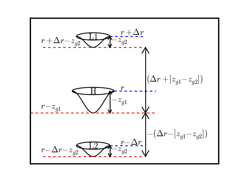
Figure 1 illustrates how gravitational redshifts act to cause an asymmetry in clustering (alongside other relativistic effects). Consider a symmetric system of three galaxies where the central galaxy () is more massive than the other two galaxies (). The distance of each of the smaller galaxies from the central galaxy is identically . Imagine that each of these galaxies is hosted by a dark matter halo which adds extra gravitational components to the measured redshifts and . If we include these effects and then examine the redshift difference of each lower mass galaxy from the central galaxy, we will find that is located at a distance and at from the central galaxy. The line of sight redshift-space distance of the two galaxies will be equal in the limit . In the scenario when the galaxies reside in haloes of different masses (different gravitational potentials) the symmetry along the line of sight will break. This effect will produce odd ordered moments in the cross-correlations of galaxies and could be used to measure the different environments of the galaxies. An important factor to note that in the autocorrelation function is that the pair counts are symmetric by construction, so no distortions of this type can be measured.
The line of sight asymmetry illustrated in Figure 1 can also be introduced by other observational effects Kaiser (2013); Bonvin et al. (2014). We have studied some of the relativistic effects on target selection (observational systematics) in a companion paper Alam et al. (2017, in press.) . A study of all such relevant effects using -body simulations is presented in another companion paper Zhu et al. (2017a, in press.). We have also investigated the effects of baryons on the gravitational potential and velocities of galaxies and their impact of relativistic distortions using hydrodynamical simulations in a third companion paper Zhu et al. (2017b, in prep.).
A outline of this paper is as follows. We provide a brief overview of our theoretical model in Section 2. Section 3 presents our dataset and Section 4 describes the steps and methods used in our measurements. The results are presented in Section 5, which include a detection of the line of sight asymmetry using large scale structure. We also discuss several null tests and systematics tests perform on the data. We conclude in section 6 with a summary and a discussion of our measurement.
2 Theory
The existence of gravitational redshift is one of the fundamental predictions of GR. As mentioned in Section 1, it has been previously studied theoretically and observed experimentally on various scales. We use -body simulations to predict the measured signal from gravitational redshifts and other effects which distort the cross-correlation function. The perturbation theory approach (e.g. McDonald, 2009; Yoo et al., 2009; Bonvin, 2014) is valid on large-scales, but non-linear clustering (including the structure of the potential well on galactic and halo scales) is dominant on the scales which are accessible to current observations ((Giusarma et al., 2017, in press.), in prep.). We therefore use N-body simulations to make predictions for the gravitational potential and velocities of galaxies. The suite of -body simulations and details of how they were used to predict different components of the signal are presented in a companion paper Zhu et al. (2017a, in press.). Here, we briefly describe the simulations and effects included in our theoretical model.
We use -body simulations produced by running the PGadget3 code (Springel et al., 2001; Springel, 2005). We use eight realizations of a flat CDM model with and . The simulations are dissipationless, in a periodic box of side length and contain particles. We use SubFind (Springel et al., 2001) to generate a catalog of subhalos which can be associated with galaxies. We then observed the subhalo catalog in the parallel line-of-sight approximation including various observational effects. We also include “wide-angle” effects which have been shown to become important on large, linear scales (Gaztanaga et al., 2015) based on linear theory prescriptions. The observed line-of-sight position is given as follows:
| (2) |
where is the final observed distance from the observer in comoving units () including all the effects we study. From now on, will denote velocity while denotes the ratio , where is the speed of light. Also, (km/s) / (h-1Mpc). The cartesian components of velocity and are indicated using subscripts (e.g., ). gives the effect of peculiar velocity on the line-of-sight distance, and is the term which causes the usual redshift distortions (e.g, (Kaiser, 1987)). The quantity is the positional shift caused by the gravitational redshift from the subhalo potential (Cappi, 1995). Two more terms introduce additional redshifts that depends on the peculiar velocity: accounts for the Transverse Doppler effect (Zhao et al., 2013) and the light cone effect (Kaiser, 2013). Because the potential well of the stellar component of the galaxy adds to the gravitational redshift, we add the component due to internal structure of galaxy similar to Cappi (1995), , where and are half-mass radius of dark matter and star particles respectively estimated from MBII hydrodynamical simulation (Khandai et al., 2015; Zhu et al., 2017b).
After adding all these components to the observed position of each galaxy in the simulation, we construct two populations of subhalos divided by median subhalo mass. The halo masses used to obtain two subsamples accounts for the luminosity distance perturbation as described in section 2.5 and specifically equation 8 of (Zhu et al., 2017a, in press.). We measure their auto-correlation functions and define two linear bias values, , and , for the high and low mass halves of the sample respectively. We compute the bias in the usual fashion (see section 4.3 for details) from the relative scaling of the large scale auto-correlation functions of subhalos and dark matter in the simulations (see (Zhu et al., 2017a, in press.) for details).
To measure the asymmetry in the cross-correlation function of the two samples we use the shell estimator, proposed by Croft (2013). This technique is simply an estimate of the centroid shift of the correlation function averaged in spherical shells, and is similar to the usual gravitational redshift profile of clusters (e.g. Wojtak et al., 2011). The shell estimator is measured from the two subsamples as follows:
| (3) |
where the sum is over all pairs of subhalos () between the two populations such that the distance between the subhalos lies in the radial bin between and . Here accounts for the relativistic beaming effect on galaxy inclusion in the sample by weighting the pair in a fashion which depends on their line of sight velocities (Kaiser, 2013; Alam et al., 2017; Iršič et al., 2016). The beaming model is derived in our companion paper (Zhu et al., 2017a, in press.) based on observational probability measured for CMASS sample in another companion paper (Alam et al., 2017, in press.). The above definition of shell estimator is equivalent to the definition given in equation 10. Lastly we add contribution of wide-angle effect to our model as described in section 2.6 of (Zhu et al., 2017a, in press.).
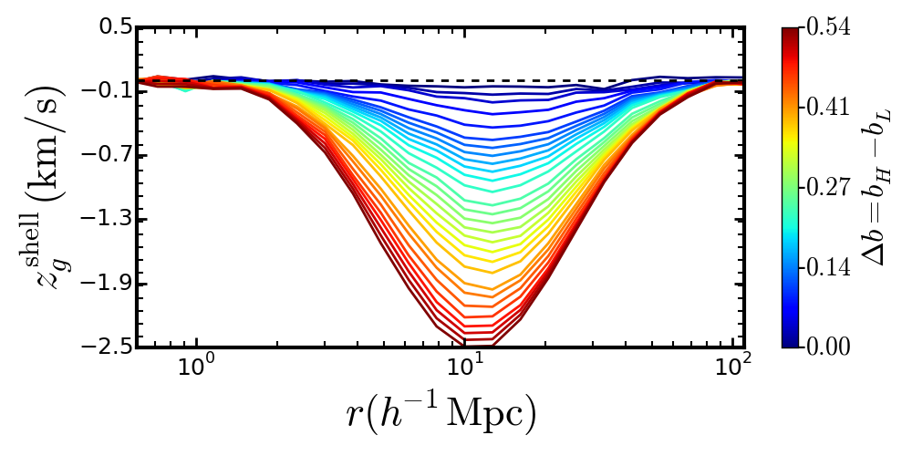
Figure 2 (top panel) shows measurements of cross-correlation function asymmetry produced by applying the shell estimator to our -body simulation outputs. Lines of different colours show measurements for various values of the large-scale bias difference between the two populations. We have used these simulation results to develop a parametric phenomenological model for the shell estimator as follows:
| (4) |
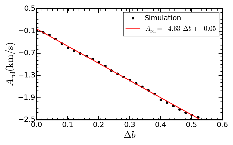
where is measured from simulations for . Here is a function of bias difference () which determines the amplitude of asymmetry. We choose for normalization because it lies in the middle of the range explored in the simulations. We have examined the amplitude as the function of bias difference from the simulations. The scaling of amplitude with bias difference is well described with a linear function.
| (5) |
The amplitude scaling of this model is motivated by the perturbation theory results; see equations 12 and 30 from Gaztanaga et al. (2015), which show that the shell estimator at linear scale should be proportional to the bias difference of the two sub-samples. Since we are working at the non-linear scale we naively expect the amplitude of the signal to depend on higher order function of linear bias difference, but the simulations show a linear scaling of amplitude with bias difference. The position of the largest asymmetry depends on the mean bias of the two populations, redshift and the relative contribution of different relativistic effects (Cai et al., 2016; Alam et al., 2017).
3 Data
To perform our measurement of relativistic distortions in the cross-correlation function we use observations from Data Release 12 (DR12;Reid et al. (2016); Alam et al. (2015a)) of the Sloan Digital Sky Survey (SDSS; York et al., 2000). SDSS I, II (Abazajian et al., 2009) and III (Eisenstein et al., 2011) used a drift-scanning mosaic CCD camera (Gunn et al., 1998) to image 14555 square degrees of the sky in five photometric bands (Fukugita et al., 1996; Smith et al., 2002; Doi et al., 2010) to a limiting magnitude of using the 2.5-m Sloan Telescope (Gunn et al., 2006) at the Apache Point Observatory in New Mexico. The imaging data were processed through a series of software pipelines (Lupton et al., 1999; Pier et al., 2003; Padmanabhan et al., 2008). Aihara et al. (2011) reprocessed all of the SDSS imaging data as part of Data Release 8 (DR8). The Baryon Oscillation Spectroscopic Survey (BOSS; Dawson et al., 2013) was designed to obtain spectra and redshifts for 1.35 million galaxies covering 10,000 square degrees of sky. These galaxies were selected from the SDSS imaging. (Blanton et al., 2003) developed a tiling algorithm for BOSS that is adaptive to the density of targets on the sky. BOSS used double-armed spectrographs Smee et al. (2013) to obtain the spectra and completed observations in spring 2014. BOSS obtained a homogeneous data set with a redshift completeness of more than 97% over the full survey footprint. The redshift extraction algorithm used in BOSS is described in Bolton et al. (2012). Eisenstein et al. (2011) provides a summary and Dawson et al. (2013) provides a detailed description of the survey design.
4 Analysis Methodology
The CMASS sample is used to define two galaxy sub-samples with different biases but same redshift distributions. We measure the auto-correlation function for each sub-sample, and estimate their linear bias values. We then measure the cross-correlation function of the two sub-samples. The cross-correlation function is used to detect and quantify the line of sight asymmetry due to relativistic effects using shell estimator of equation 10. In this section we describe our analysis methodologies in detail.
4.1 Creating Galaxy sub-samples
The SDSS CMASS DR12 sample of galaxies are used create two sub-samples of galaxies that occupy lower and higher mass halos. We use galaxy absolute magnitude to divide the overall sample into these two subsamples, making the assumption that more luminous galaxies are associated with higher mass, and consequently higher bias halos van Uitert et al. (2015). We use five different approaches to divide the dataset into two sub-samples, using magnitude in the five different SDSS bands.
Our procedure is as follows: We first bin the sample into redshift bins with . In each bin, we compute the median magnitude for one of the five photometric bands (). Galaxies brighter than the median magnitude in the bin are placed into the bright subsample and fainter galaxies in the faint subsample. We repeat the process for the other four photometric bands so that we have five different partitions of the whole dataset into bright and faint subsamples. This process guarantees that the two sub-samples have same redshift distribution. Our measurements are not sensitive to choice of , we provide more details of this approach and other tests in section 5.5 and Figure 10.
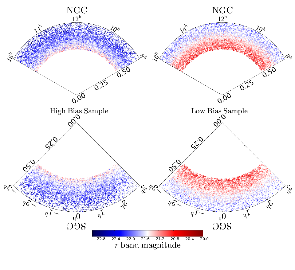
The photometric band magnitudes used in our analysis are adjusted for evolution and the k-correction to . We did not account for error on the magnitudes which will lead to a scatter in the galaxy around the dividing magnitude. The faint sub-sample contains 382,711 galaxies and the bright sub-sample contains 382,722 galaxies, when band magnitudes are used to define the cut. Figure 3 shows the distribution of galaxies in right ascension and distance from the observer in these two CMASS subsamples. We obtain similar samples using the other photometric bands.
4.2 Estimating the cross-correlation function
We adopt as a fiducial cosmology a flat CDM-GR cosmological model with , ,, and (Anderson et al., 2014) in order to convert observed celestial coordinates () and redshift to the position of the galaxy in three-dimensional space. These galaxy positions are used to estimate the two point statistic (cross-correlation function) of the galaxies in the two subsamples using the minimum variance, Landy-Szalay estimator (Landy & Szalay, 1993):
| (6) | |||
Here and represent, respectively, the weighted counts of galaxy pairs from the two populations, pairs of galaxies in the first population with randoms for the second population, randoms for first population with galaxies from the second population and between randoms for two populations. We use the weighting scheme described in Anderson et al. (2014) to account for systematic weights of the individual galaxies. The weight factor accounts for redshift failure of the nearest neighbor of a galaxy. The weight factor is intended to account for a scenario where the redshift of a neighbor was not obtained because it was in a close pair due to fiber collision. The weights and account for stellar density and the seeing effect in the galaxy sample.
The cross-correlation function depends on , the distance between a pair of galaxies, and , where is the angle between the pair separation vector and the line of sight. We define the line-of-sight direction for each pair to be the position vector that joins the observer to the mean position of that pair of galaxies. We carry out cross-correlation function measurements covering 1 h-1Mpc 60 h-1Mpc with 15 logarithmic bins and with 150 linear bins. Provided that the binning is not much finer or coarser than these values our measurements are insensitive to binning choices.
4.3 Estimating Multipoles and Galaxy bias
We measure the 2D cross-correlation function from the CMASS data as described in section 4.2. We compress the cross-correlation by projecting it onto a basis of Legendre polynomials of order as follows:
| (7) | ||||
| (8) |
where . The moments of the Legendre polynomials are given by , the monopole, dipole and quadrupole, respectively. We estimate the linear bias of a sample of galaxies by fitting the model to the observed monopole from data. Convolution Lagrangian Perturbation Theory (CLPT; Carlson et al., 2013) is used to estimate the monopole of the matter correlation function () assuming fiducial cosmology for . We also estimate the dipole moment and use it as a means to detect asymmetry in the cross-correlation function Gaztanaga et al. (2015).
4.4 Estimating the Covariance Matrix
Estimation of the covariance matrix of a summary statistic (such as the cross-correlation function) is one of the most important steps in a cosmological analysis. The covariance matrix of an observed statistic is usually computed either by sub-sampling the data or by using mock catalogues. Both methods have their limitations and regime of validity. Generally speaking, the sub-sampling methods over-estimate errors on small scale (Norberg et al., 2009) and are difficult to use on large scales due to the limited volume of the observed data. Conversely creating realistic mock catalogues in large numbers and covering a large volume with high spatial resolution requires huge computing resources. Therefore, mocks often use approximate simulations with lower spatial and temporal resolution (e.g. White et al., 2014). This approach makes small scale clustering in the mocks inaccurate and hence covariance estimated from mocks can only be used above a certain minimum scale decided by details of the method.
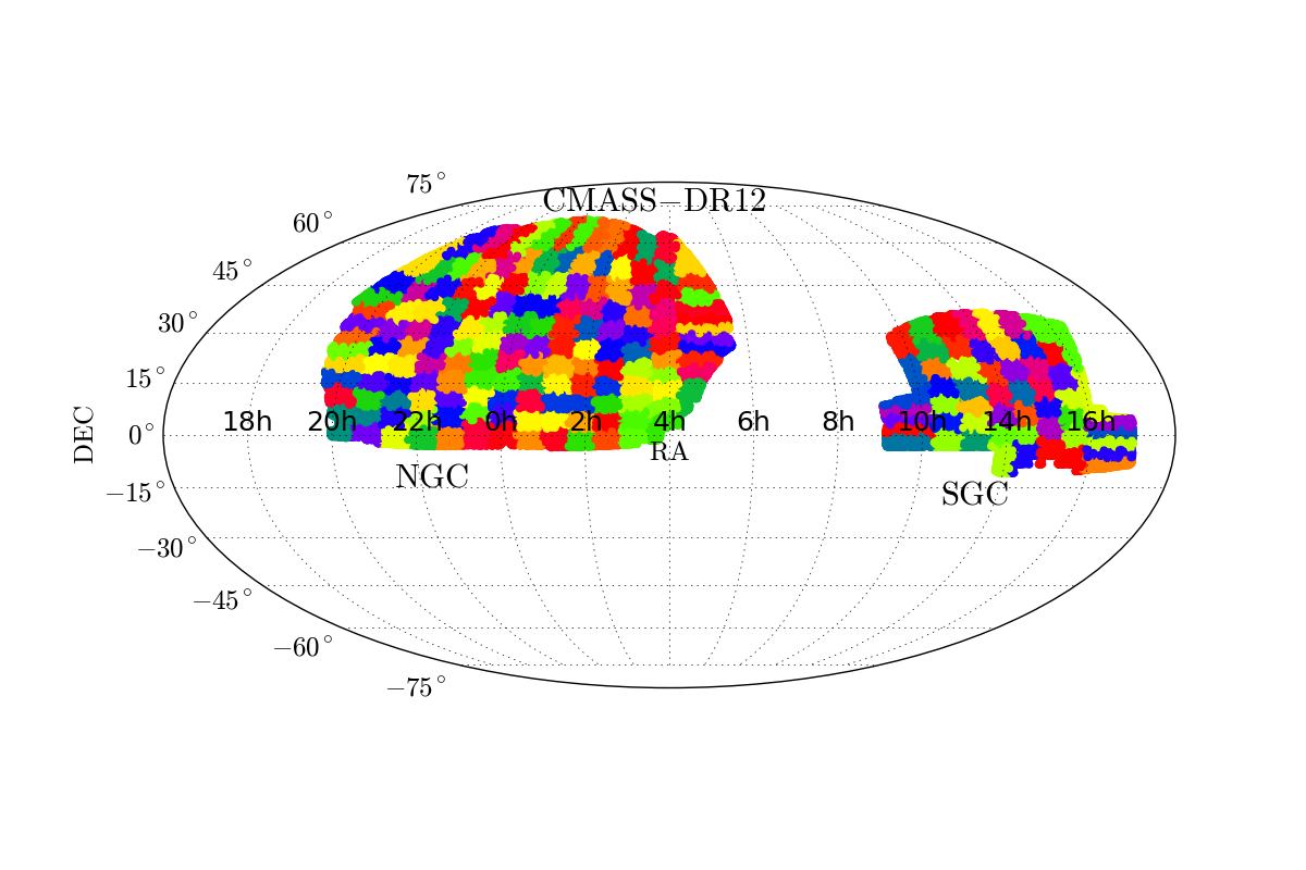
Because our signal of interest is on small scales (h-1Mpc) we adopt the subsampling approach. We use the “delete one jackknife” algorithm (Shao, 1986) to estimate the covariance matrix. We first split the data into 210 approximately equal area regions (154 in the North Galactic cap and 56 in the South Galactic cap) as shown in Figure 4. A realization of data is defined by omitting one region at a time, which yields 210 realizations. We measure the summary statistics, correlation function and shell estimator for each realization. We then estimate the covariance matrix of these summary statistics () using
| (9) |
Here represents the covariance between bin and , is the mean of the jackknife realizations and the sum is over all the 210 jackknife realizations. Our smallest jackknife region has an angular diameter of , which translates to h-1Mpc. This distance is much larger than largest scale we are using in our analysis.
4.5 Shell estimator: Estimating Asymmetry
As our primary measure of the redshift asymmetry in clustering caused by relativistic effects, we use a shell-averaged estimator applied to the cross-correlation function. Croft (2013) proposed this estimator to quantify the effects of gravitational redshift predicted from in -body simulations. The shell estimator is defined as follows:
| (10) |
where is the angle of pair separation from line of sight. We can see that measures the mean weighted by the cross correlation function and is converted to km/s units through multiplication factor of H=100 (km/s) / (h-1Mpc). Other quantifications of the relativistic asymmetry in clustering have been proposed, such as the imaginary part of the power spectrum McDonald (2009), the dipole Bonvin et al. (2014), and the anti-symmetric part of the cross-correlation function Iršič et al. (2016). Here we focus on the shell estimator, but also measure the dipole and compare conclusions derived from both.
5 Measurements, Null Tests and Systematics
We use the methodologies described in previous section to perform our clustering measurements. In this section we present the measurement of bias, the measurements of shell estimator and fitting the model described in section 2. We also perform two null tests and look at the sensitivity of our observed signal to the possible systematic.
5.1 Measurements of Bias
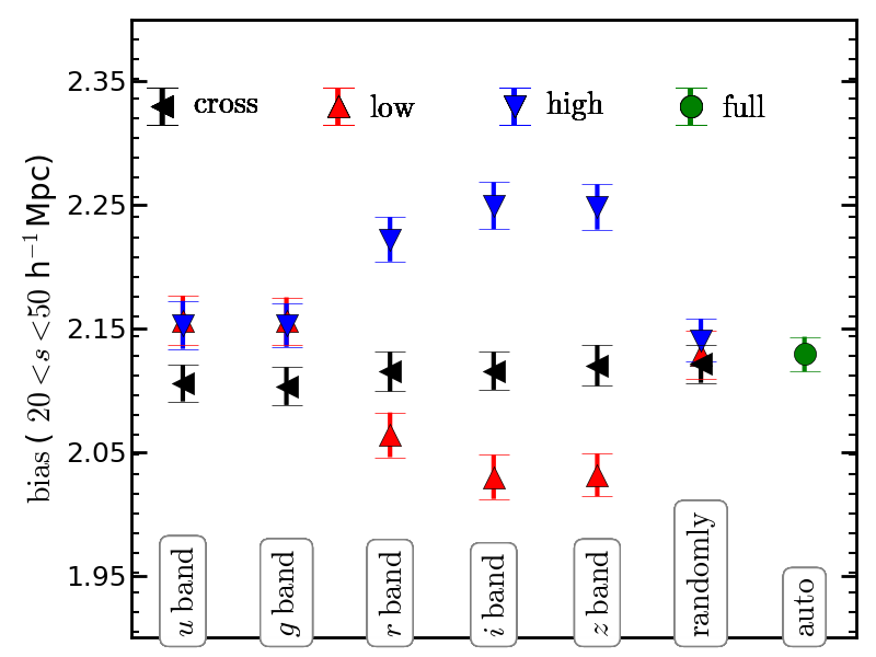
The linear biases measured for our various samples are displayed in Figure 5. The galaxy bias is measured using the monopole as described in section 4.3. We use scales between 20h-1Mpc and 50h-1Mpc to measure bias. The bias of auto-correlation and cross-correlation of different sub-samples created by splitting the sample using all five photometric bands () and randomly are presented in the figure. The blue points show the biases of higher mass samples, red points for lower mass samples and the black points for the cross-correlation between the lower and higher mass samples. The bias of full sample is indicated by the green point. The relativistic effects, dominantly the gravitational redshift, breaks the line of sight symmetry of cross-correlation and is proportional to the difference in biases of the two sub-samples. Therefore we expect to see relatively smaller signal for and bands and relatively larger signal for and bands. We also expect no line of sight asymmetry in the cross-correlation using random split and the auto-correlation of the full sample. These two cases are used as our null tests.
5.2 Measurements of the shell estimator
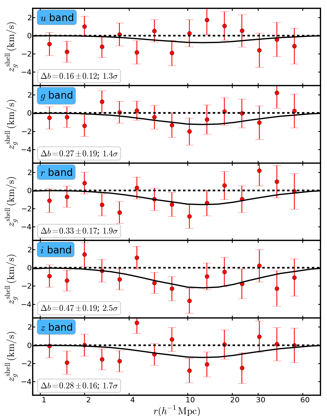
Figure 6 presents the measurements of the shell estimator together with the best fit model. The red points show our measurement of the asymmetry which we interpret as being due to relativistic effects including gravitational redshift (). The solid black lines indicate the expected signal based on our best fit model. We have used predictions from -body simulation to fit the measurements for each band using the model described in equation 4. Our likelihood function is defined as follows
| (11) | |||
| (12) |
where represents the inverse of the covariance matrix obtained from jacknife sampling as shown in equation 9. The likelihood is used to estimate the mean and error on measured from the model fit. This value of is therefore the one inferred from the clustering asymmetry, assuming relativistic effects. It can be compared to the value of directly measured from the ratio of the galaxy correlation functions, to see if they are consistent.
The requirement that the amplitude of the line-of-sight asymmetry approaches zero () in the absence of any relativistic effects is our null hypothesis. The detection significance quantifies the difference of bias difference from zero in units of standard error (). We fit only for the amplitude of asymmetry as the function of . Table 1 provides the results of our fits for each of the photometric band. The best fit model is shown in Figure 6 with the black solid line. The measured bias difference (), its error and detection significance, are also given in Figure 6.
| [0.0] | ||
| [0.0] | ||
| [0.16] | ||
| [0.23] | ||
| [0.21] | ||
| [0.01] | ||
The and bands show an amplitude of gravitational redshift consistent with zero, which is expected given that the bias difference of the two sub-samples using these bands is small. The and bands have a deviation of from zero at the and levels, respectively. If we compare the bias difference measured from the shell estimator (largely from non-linear scales) and from monopole of the correlation function we find consistency at the level or better.
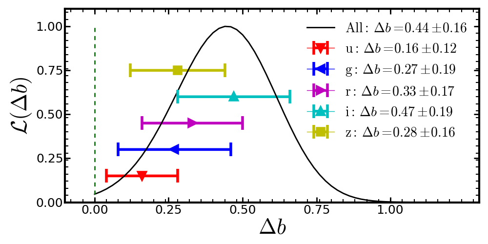
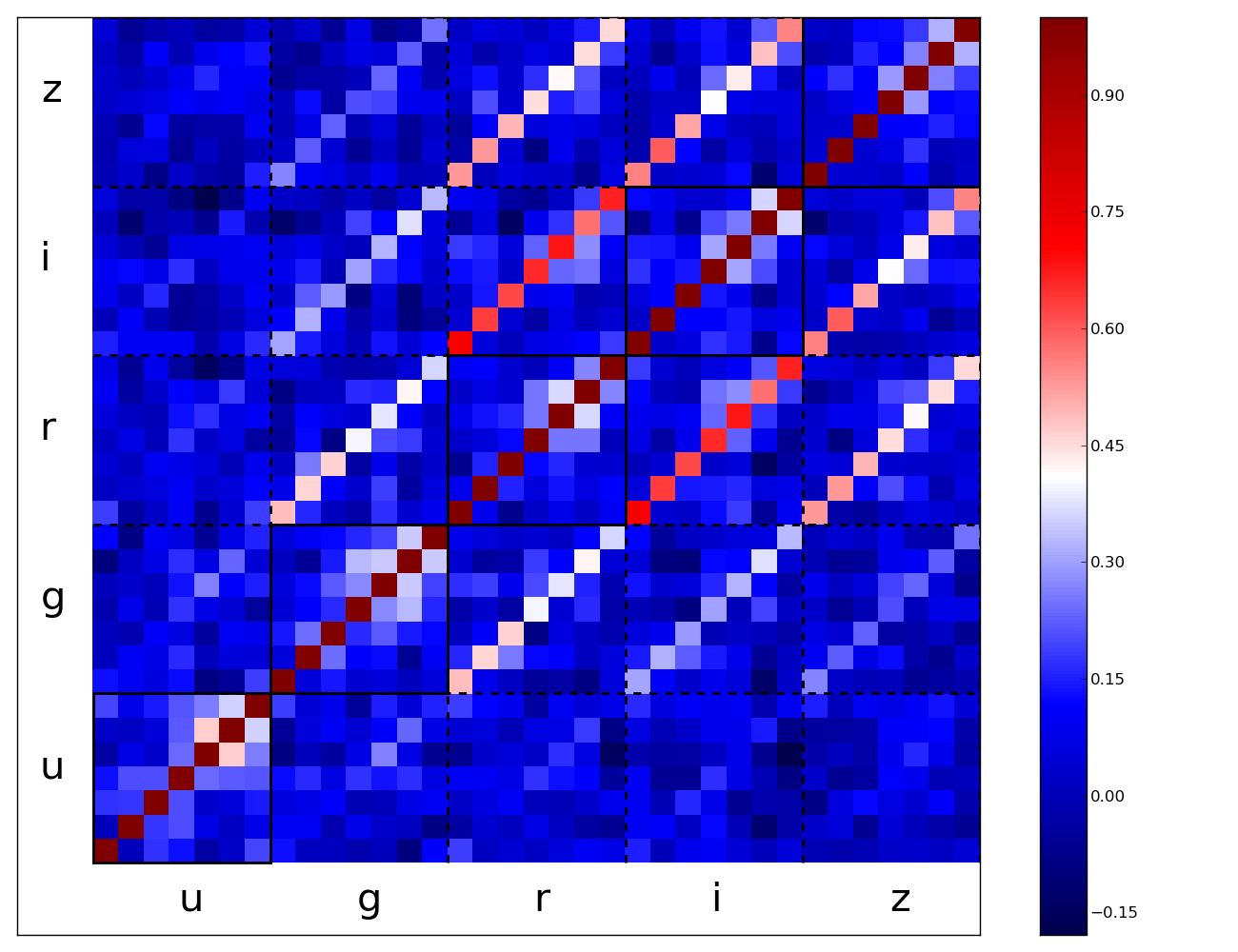
We have also performed a simultaneous fit to all five bands accounting for the cross-correlation between the bands. We fit for one corresponding to band and scale the models for the other bands by the ratio of the best fit of the band to that for the band. In order to be able to compute the covariance matrix among different bands we use only the central 7 bins of the measured values, covering scales between 3 to 25 h-1Mpc. This combined measurement yields a 2.7 detection with . Figure 7 shows the likelihood and correlation matrix. The black line in the top plot shows the likelihood when combining all 5 bands and the individual points shows the measurements for the individual band fits. The bottom plot shows the normalised covariance matrix within the band and across the band. We can see that as expected there is strong covariance, particularly between bins at the same scale in different bands (up to covariance). As a result there is only marginal improvement in the significance of the measurement from combining the different bands.
5.3 Null Tests
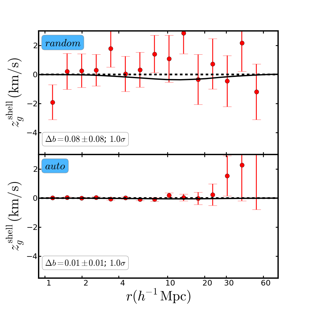
We perform two null tests to check for systematics. First, we divide the sample randomly in two equal halves and examine the shell estimator from the cross-correlation of the two random sub-samples. We do not expect to observe any signal showing line of sight asymmetry from such a measurement, because the two sub-samples are statistically same. The top panel in Figure 8 shows the shell estimator measurement from the random split. We obtained which is consistent with zero signal at the level. We have also investigated the shell estimator from the auto-correlation of the full sample, which serves as the second null test. The bottom panel in Figure 8 shows the measurement of the shell estimator from the auto-correlation of the full sample. This analysis yields , which is consistent with zero at the level. Any problems with the survey geometry, mask, large angle effect or redshift distribution should produce a non-zero signal in at least one of these measurements. Note that null test using the auto-correlation has a much smaller error bar and still produces a null result which is a strong test for many of the possible systematic effects. Both of our null tests are in excellent agreement and suggest that our analysis is not affected with significant systematic effects.
5.4 Measurement of Dipole moment
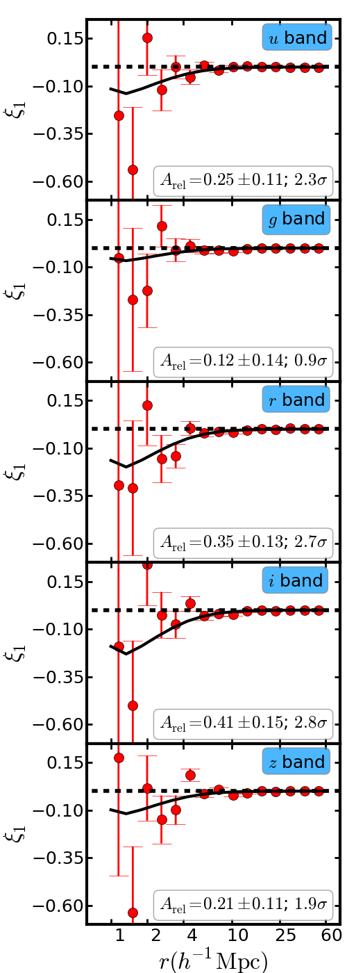
We have measured the dipole moment of the cross-correlation for each of the photometric band as described in section 4.3; Figure 9 presents these results. Each panel shows the dipole moment of the cross-correlation for each of the photometric bands. The red points indicate our measurement with a jackknife error bar. The black line represents the best fit halo model prediction. The reader is referred to Croft (2013) for details of halo model used for the dipole moment, and for evidence that the model reproduces simulation results. Briefly, the model estimates the mass function as the integral of the difference between galaxy matter correlation function for the two sub-samples and uses the mass function to estimate the gravitational redshift in the context of general relativity (see equations 2 and 3 of Croft (2013)). The results shown here for the dipole are included to show that asymmetry can be measured using a different statistic than the shell estimator. We present the shell estimator as our primary result because in our companion paper ((Zhu et al., 2017a, in press.)) we found making simulation predictions for the dipole including all relativistic effects to be technically unfeasible.
We fit the halo model prediction for a constant amplitude which is a multiplicative factor to our fiducial halo model prediction. The dipole moment shows a non-zero signal at small scales similar to the shell estimator. The figure also shows the best fit value of the halo model amplitude. We detect the amplitude of relativistic asymmetry at the level of ,, , and in the and bands, respectively, but do not detect any dipole signal at large scale. The results are entirely consistent with zero for scales above 25h-1Mpc.
5.5 Sensitivity to Systematics
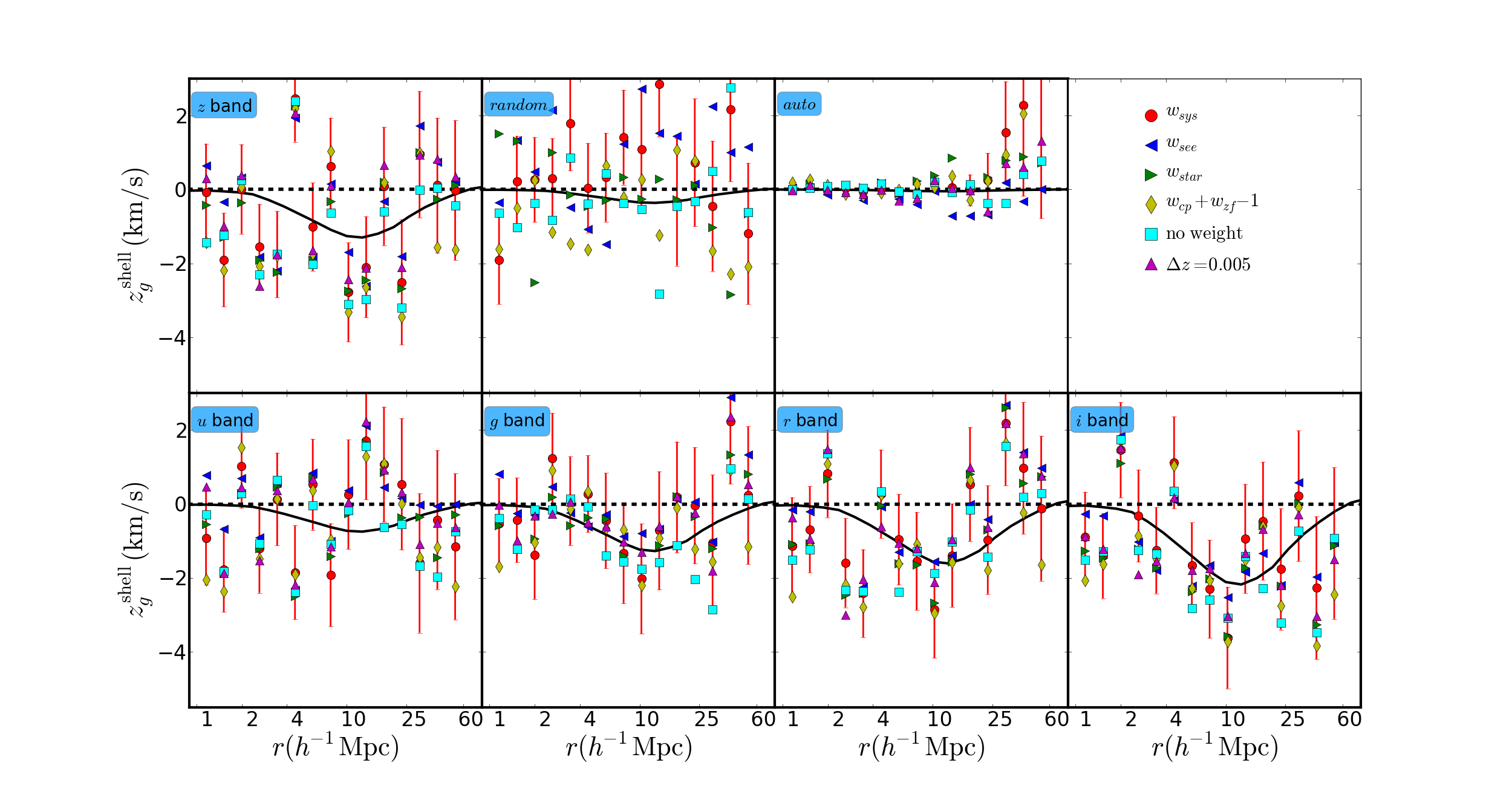
We have used the systematic weights suggested in the catalog in an attempt to remove any observational correlation that shouldn’t exist in our samples. We apply five combinations of systematic weights, as listed in the legend of Figure 10, in the measurement of cross-correlation for each of the photometric bands and null tests. We compute the shell estimator for each of these weights for each sub-samples, produces 35 different measurements, which are all displayed in Figure 10. The seven different panels show the shell estimator measurement for each photometric bands and also the ones used for our null-tests. The coloured points represent different combinations of systematic weights used in the correlation function measurement. The red points in each panel are our fiducial measurement. We found that the effect of any of these systematic weights are small, and obtain consistent measurement within independent of what systematic weights are used. This exercise demonstrate that our measurements are robust against observational systematic. We have also tested the effect of redshift binning while creating the sub-samples. Our fiducial bin width is , as shown using red points. Decreasing the bin width to , as shown using magenta points, does not change the measurement significantly. The fact that our measurements is not sensitive to the combination of weights used or choice of redshift binning suggests that it may be stable against lack of detailed understanding of some of these systematic weights.
6 Discussion
We have discussed various relativistic effects which could produce line-of-sight asymmetries in the cross-correlation of two galaxy populations with different mean halo mass and used the BOSS CMASS sample to measure these asymmetries. We used each of the five SDSS photometric bands in turn to obtain five sets of two sub-samples. The galaxy biases of these sub-samples were measured by measuring the monopole of auto- and cross-correlation as described in section 4.3 and shown in Figure 5. The shell estimator described in section 4.5 was used to quantify the line-of-sight anisotropy due to the relativistic effects in velocity units. We have used a model developed using -body simulations and motivated by perturbation theory to fit the measured shell-estimator. The theoretical model for shell estimator is described in section 2 and derived from the analysis of a companion paper Zhu et al. (2017a, in press.). The theoretical model was fit to measurements from data in order to quantify the significance of observed signal. The covariance matrix which estimates the uncertainties was obtained using jackknife sampling as described in section 4.4. Figure 6 shows our measurements with best fit models and detection significance. We detect the amplitude of relativistic asymmetry at the level of , and away from zero in the and bands respectively. This result is consistent with our expectation from the relative bias measurements of the five sub-samples as shown in Figure 5. The amplitude of relativistic asymmetry for the and bands are at the level of and , consistent with the expectation from biases. We detect the signal at 2.7 after combining the measurements from all 5 bands including the cross-covariance (using only the central 7 bins covering scales between 3 to 25 h-1Mpc.)
Zhu et al. (2017a) found that the dominant contribution in the shell estimator is due to the gravitational redshift effects. Therefore our measured signal can be seen as a first detection of gravitational redshifts distorting the large scale structure of the Universe. Two null tests were devised to check the possibility that the measured line-of-sight asymmetry is due to the survey geometry, mask effects, large angle effects, redshift distribution, etc. The first null test measures the shell estimator from the cross-correlation of two randomly selected galaxy populations. This procedure makes the two populations statistically identical and hence we do not expect any line-of-sight-anisotropy in the cross-correlation. The second null test uses the shell estimator measured from the auto-correlation of the full sample. This test has much smaller error, allowing to check for possible geometrical effects to much higher precision than the statistical uncertainty in our measurement. Figure 10 demonstrates that our null tests are consistent with zero, implying that any of those possible systematic effects lie significantly below our statistical uncertainty. We have also performed a much more detailed analysis of possible systematic effects due to sample selection in the companion paper Alam et al. (2017, in press.).
Another avenue to quantify the line-of-sight asymmetry is the dipole moment of the cross-correlation function (described in section 4.3 and shown in Figure 9). We found similar levels of asymmetry on small scales to those found with the shell estimator. We fit our dipole moments using the prediction from halo model described in Croft (2013), and detect the amplitude of relativistic asymmetry at the significance level of ,, , and in the and bands respectively. Differences between the two measurements are likely caused by the fact that the shell estimator and dipole moment weight the clustering modes differently. Our dipole moments are completely consistent with zero on large scales. This result is also consistent with the analysis presented by Gaztanaga et al. (2015), who did not detect any signal using dipole moment and shell estimator on large scales. We used a halo model to measure the dipole moment signal; this model is not as rigorously tested as our model for the shell estimator based on simulations. A better understanding of dipole moment models based on analytical methods or simulation will be a necessary step for the future work on the measurement of relativistic asymmetry.
This first detection of gravitational redshifts using large scale structure can be regarded another success for General Relativity, however, we have found in companion work (including Zhu et al., 2017a, in press.) that there are significant uncertainties in the theoretical predictions for relativistic distortions, particularly related to the role of structure on galactic scales. The observational measurements, from large-scale galaxy clustering in this paper, and from galaxy clusters (e.g. Wojtak et al., 2011; Sadeh et al., 2015) are also currently at only the 2-3 of significance. Future surveys with greater volume and larger numbers of galaxies will be able to detect such signals with much higher significance. Such surveys will not only look at much larger volumes but also probe much deeper, covering a wider variety of galaxies and greater differences in the relative biases of samples. These surveys, including ongoing programs such as eBOSS and future projects such as DESI and Euclid, are already developing large simulations and suites of analysis tools which will be available for relativistic clustering studies. These efforts have the potential to bring these distortions of large-scale structure into the realm of precision cosmology and allow unprecedented tests of General Relativity.
Acknowledgments
We would like to thank Nick Kaiser for many insightful discussions during the course of this project. This work was supported by NSF grant AST1412966. SA and SH are supported by NASA grants 12-EUCLID11-0004. SA is also supported by the European Research Council through the COSFORM Research Grant(#670193). We would like to thank Ayesha Fatima for going through the early draft and helping us making the text much more clear.
SDSS-III is managed by the Astrophysical Research Consortium for the Participating Institutions of the SDSS-III Collaboration including the University of Arizona, the Brazilian Participation Group, Brookhaven National Laboratory, Carnegie Mellon University, University of Florida, the French Participation Group, the German Participation Group, Harvard University, the Instituto de As trofisica de Canarias, the Michigan State/Notre Dame/JINA Participation Group, Johns Hopkins University, Lawrence Berkeley National Laboratory, Max Planck Institute for Astrophysics, Max Planck Institute for Extraterrestrial Physics, New Mexico State University, New York University, Ohio State University, Pennsylvania State University, University of Portsmouth, Princeton University, the Spanish Participation Group, University of Tokyo, University of Utah, Vanderbilt University, University of Virginia, University of Washington, and Yale University.
References
- Abazajian et al. (2009) Abazajian K. N., et al., 2009, ApJS, 182, 543
- Abbott et al. (2016) Abbott B. P., et al., 2016, Phys. Rev. Lett., 116, 061102
- Aihara et al. (2011) Aihara H., et al., 2011, ApJS, 193, 29
- Alam et al. (2015a) Alam S., Albaret F. D., Prieto C. A., 2015a, ApJS
- Alam et al. (2015b) Alam S., Ho S., Vargas-Magaña M., Schneider D. P., 2015b, MNRAS, 453, 1754
- Alam et al. (2016) Alam S., Ho S., Silvestri A., 2016, MNRAS, 456, 3743
- Alam et al. (2017) Alam S., Croft R. A. C., Ho S., Zhu H., E. G., 2017, xxx, pp xx–xx
- Anderson et al. (2014) Anderson L., et al., 2014, MNRAS, 441, 24
- Beutler et al. (2012) Beutler F., et al., 2012, MNRAS, 423, 3430
- Beutler et al. (2014) Beutler F., et al., 2014, MNRAS, 443, 1065
- Blake et al. (2011a) Blake C., et al., 2011a, MNRAS, 415, 2876
- Blake et al. (2011b) Blake C., et al., 2011b, MNRAS, 418, 1707
- Blanton et al. (2003) Blanton M. R., Lin H., Lupton R. H., Maley F. M., Young N., Zehavi I., Loveday J., 2003, AJ, 125, 2276
- Bolton et al. (2012) Bolton A. S., et al., 2012, AJ, 144, 144
- Bonvin (2014) Bonvin C., 2014, Classical and Quantum Gravity, 31, 234002
- Bonvin et al. (2014) Bonvin C., Hui L., Gaztañaga E., 2014, Phys. Rev. D, 89, 083535
- Cai et al. (2016) Cai Y.-C., Kaiser N., Cole S., Frenk C., 2016, preprint, (arXiv:1609.04864)
- Cappi (1995) Cappi A., 1995, A&A, 301, 6
- Carlson et al. (2013) Carlson J., Reid B., White M., 2013, MNRAS, 429, 1674
- Clemence (1947) Clemence G. M., 1947, Reviews of Modern Physics, 19, 361
- Colless et al. (2003) Colless M., et al., 2003, preprint, (arXiv:astro-ph/0306581)
- Croft (2013) Croft R. A. C., 2013, MNRAS, 434, 3008
- Dawson et al. (2013) Dawson K. S., et al., 2013, AJ, 145, 10
- Doi et al. (2010) Doi M., et al., 2010, AJ, 139, 1628
- Dyson et al. (1920) Dyson F. W., Eddington A. S., Davidson C., 1920, Philosophical Transactions of the Royal Society of London A: Mathematical, Physical and Engineering Sciences, 220, 291
- Einstein (1916) Einstein A., 1916, Annalen Der Physik, 49, 770
- Eisenstein et al. (2011) Eisenstein D. J., et al., 2011, AJ, 142, 72
- Fukugita et al. (1996) Fukugita M., Ichikawa T., Gunn J. E., Doi M., Shimasaku K., Schneider D. P., 1996, AJ, 111, 1748
- Garilli et al. (2014) Garilli B., et al., 2014, A&A, 562, A23
- Gaztanaga et al. (2015) Gaztanaga E., Bonvin C., Hui L., 2015, preprint, (arXiv:1512.03918)
- Giusarma et al. (2017) Giusarma E., Alam S., Zhu H., Croft R. A. C., Ho S., 2017, xxx, pp xx–xx
- Greenstein et al. (1971) Greenstein J. L., Oke J. B., Shipman H. L., 1971, ApJ, 169, 563
- Gunn et al. (1998) Gunn J. E., et al., 1998, AJ, 116, 3040
- Gunn et al. (2006) Gunn J. E., et al., 2006, AJ, 131, 2332
- Hamilton (1992) Hamilton A. J. S., 1992, ApJ, 385, L5
- Howlett et al. (2015) Howlett C., Ross A. J., Samushia L., Percival W. J., Manera M., 2015, MNRAS, 449, 848
- Iršič et al. (2016) Iršič V., Di Dio E., Viel M., 2016, J. Cosmology Astropart. Phys., 2, 051
- Jeong et al. (2012) Jeong D., Schmidt F., Hirata C. M., 2012, Phys. Rev. D, 85, 023504
- Jimeno et al. (2015) Jimeno P., Broadhurst T., Coupon J., Umetsu K., Lazkoz R., 2015, MNRAS, 448, 1999
- Jones et al. (2009) Jones D. H., et al., 2009, MNRAS, 399, 683
- Kaiser (1987) Kaiser N., 1987, MNRAS, 227, 1
- Kaiser (2013) Kaiser N., 2013, MNRAS, 435, 1278
- Kennefick (2007) Kennefick D., 2007, preprint, (arXiv:0709.0685)
- Khandai et al. (2015) Khandai N., Di Matteo T., Croft R., Wilkins S., Feng Y., Tucker E., DeGraf C., Liu M.-S., 2015, MNRAS, 450, 1349
- Kim & Croft (2004) Kim Y.-R., Croft R. A. C., 2004, ApJ, 607, 164
- Landy & Szalay (1993) Landy S. D., Szalay A. S., 1993, ApJ, 412, 64
- Liske et al. (2015) Liske J., et al., 2015, MNRAS, 452, 2087
- Lopresto et al. (1991) Lopresto J. C., Schrader C., Pierce A. K., 1991, ApJ, 376, 757
- Lupton et al. (1999) Lupton R. H., Gunn J. E., Szalay A. S., 1999, AJ, 118, 1406
- McDonald (2009) McDonald P., 2009, J. Cosmology Astropart. Phys., 11, 026
- Newman et al. (2013) Newman J. A., et al., 2013, ApJS, 208, 5
- Norberg et al. (2009) Norberg P., Baugh C. M., Gaztañaga E., Croton D. J., 2009, MNRAS, 396, 19
- Nordtvedt (1968a) Nordtvedt K., 1968a, Physical Review, 169, 1017
- Nordtvedt (1968b) Nordtvedt K., 1968b, Physical Review, 170, 1186
- Nordtvedt (1985) Nordtvedt K., 1985, ApJ, 297, 390
- Padmanabhan et al. (2008) Padmanabhan N., et al., 2008, ApJ, 674, 1217
- Peebles (1980) Peebles P. J. E., 1980, The large-scale structure of the universe
- Percival et al. (2004) Percival W. J., et al., 2004, MNRAS, 353, 1201
- Pier et al. (2003) Pier J. R., Munn J. A., Hindsley R. B., Hennessy G. S., Kent S. M., Lupton R. H., Ivezić Ž., 2003, AJ, 125, 1559
- Pound & Rebka (1959) Pound R. V., Rebka G. A., 1959, Phys. Rev. Lett., 3, 439
- Pullen et al. (2015a) Pullen A. R., Alam S., He S., Ho S., 2015a, preprint, (arXiv:1511.04457)
- Pullen et al. (2015b) Pullen A. R., Alam S., Ho S., 2015b, MNRAS, 449, 4326
- Reid et al. (2012) Reid B. A., et al., 2012, MNRAS, 426, 2719
- Reid et al. (2014) Reid B. A., Seo H.-J., Leauthaud A., Tinker J. L., White M., 2014, MNRAS, 444, 476
- Reid et al. (2016) Reid B., et al., 2016, MNRAS, 455, 1553
- Reyes et al. (2010) Reyes R., Mandelbaum R., Seljak U., Baldauf T., Gunn J. E., Lombriser L., Smith R. E., 2010, Nature, 464, 256
- Sadeh et al. (2015) Sadeh I., Feng L. L., Lahav O., 2015, Physical Review Letters, 114, 071103
- Samushia et al. (2012) Samushia L., Percival W. J., Raccanelli A., 2012, MNRAS, 420, 2102
- Sánchez et al. (2013) Sánchez A. G., et al., 2013, MNRAS, 433, 1202
- Schneider (2005) Schneider P., 2005, ArXiv Astrophysics e-prints,
- Shao (1986) Shao J., 1986, Ann. Statist., 14, 1322
- Shapiro (1964) Shapiro I. I., 1964, Physical Review Letters, 13, 789
- Simpson et al. (2016) Simpson F., et al., 2016, Phys. Rev. D, 93, 023525
- Smee et al. (2013) Smee S. A., et al., 2013, AJ, 146, 32
- Smith et al. (2002) Smith J. A., Tucker D. L., Allam S. S., Jorgensen A. M., 2002, in American Astronomical Society Meeting Abstracts. p. #104.08
- Springel (2005) Springel V., 2005, MNRAS, 364, 1105
- Springel et al. (2001) Springel V., Yoshida N., White S. D. M., 2001, New Astron., 6, 79
- Takeda & Ueno (2012) Takeda Y., Ueno S., 2012, Sol. Phys., 281, 551
- Weisberg et al. (1981) Weisberg J. M., Taylor J. H., Fowler L. A., 1981, Scientific American, 245, 74
- White et al. (2014) White M., Tinker J. L., McBride C. K., 2014, MNRAS, 437, 2594
- Wojtak et al. (2011) Wojtak R., Hansen S. H., Hjorth J., 2011, Nature, 477, 567
- Yoo (2014) Yoo J., 2014, Classical and Quantum Gravity, 31, 234001
- Yoo & Zaldarriaga (2014) Yoo J., Zaldarriaga M., 2014, Phys. Rev. D, 90, 023513
- Yoo et al. (2009) Yoo J., Fitzpatrick A. L., Zaldarriaga M., 2009, Phys. Rev. D, 80, 083514
- Yoo et al. (2012) Yoo J., Hamaus N., Seljak U., Zaldarriaga M., 2012, Phys. Rev. D, 86, 063514
- York et al. (2000) York D. G., et al., 2000, AJ, 120, 1579
- Zhang et al. (2007) Zhang P., Liguori M., Bean R., Dodelson S., 2007, Physical Review Letters, 99, 141302
- Zhao et al. (2013) Zhao H., Peacock J. A., Li B., 2013, Phys. Rev. D, 88, 043013
- Zhu et al. (2017b) Zhu H., Alam S., Croft R. A. C., Ho S., E. G., 2017b, xxx, pp xx–xx
- Zhu et al. (2017a) Zhu H., Alam S., Croft R. A. C., Ho S., E. G., 2017a, xxx, pp xx–xx
- de la Torre et al. (2013) de la Torre S., et al., 2013, A&A, 557, A54
- van Uitert et al. (2015) van Uitert E., Cacciato M., Hoekstra H., Herbonnet R., 2015, A&A, 579, A26