Extension of holomorphic motions
and monodromy

Abstract.

Let $E$ be a closed set in the Riemann sphere $\widehat{\mathbb{C}}$. We consider a holomorphic motion $\phi$ of $E$ over a complex manifold $M$, that is, a holomorphic family of injections on $E$ parametrized by $M$. It is known that if $M$ is the unit disk $\Delta$ in the complex plane, then any holomorphic motion of $E$ over $\Delta$ can be extended to a holomorphic motion of the Riemann sphere over $\Delta$.

In this paper, we consider conditions under which a holomorphic motion of $E$ over a non-simply connected Riemann surface $X$ can be extended to a holomorphic motion of $\widehat{\mathbb{C}}$ over $X$. Our main result shows that a topological condition, the triviality of the monodromy, gives a necessary and sufficient condition for a holomorphic motion of $E$ over $X$ to be extended to a holomorphic motion of $\widehat{\mathbb{C}}$ over $X$.

We give topological and geometric conditions for a holomorphic motion over a Riemann surface to be extended. We also apply our result to a lifting problem for holomorphic maps to Teichmüller spaces.

1. Introduction

A family of injections depending holomorphically on complex parameters is called a holomorphic motion (see Definition 2.1 for the precise definition), which is a powerful tool for complex dynamics, the deformation theory of Kleinian groups and Teichmüller theory. It first appeared in the $\lambda$-lemma of a paper [17] by Mané, Sad and Sullivan. The lemma says that every holomorphic motion of a set $E$ in the Riemann sphere $\widehat{\mathbb{C}}$ is extended to a holomorphic motion of the closure of $E$. Since then, the theory of holomorphic motions has been rapidly developed.

In fact, the $\lambda$-lemma was improved by Bers-Royden([3]) and Sullivan-Thurston ([26]); Slodkowski ([24], [25]) showed that every holomorphic motion of a closed set in $\widehat{\mathbb{C}}$ over the unit disk $\Delta\subset\mathbb{C}$ is extended to a holomorphic motion of $\widehat{\mathbb{C}}$ over $\Delta$. Moreover, Earle, Kra and Krushkal ([8]) proved that if a holomorphic motion over $\Delta$ is $G$-equivariant for a subgroup $G$ of Möbius transformations (see Definition 2.2), then it is extended to a holomorphic motion of $\widehat{\mathbb{C}}$ which is also $G$-equivariant.

On the other hand, if the parameter space of a holomorphic motion is not simply connected, then the holomorphic motion cannot be extended to a holomorphic motion of $\widehat{\mathbb{C}}$ in general (see [2] for related results).

In this paper, we consider conditions of a holomorphic motion over a non-simply connected Riemann surface $X$ under which the holomorphic motion can be extended to a holomorphic motion of $\widehat{\mathbb{C}}$ over $X$. In fact, we give a necessary and sufficient condition for a holomorphic motion over a Riemann surface to be extended to a holomorphic motion of $\widehat{\mathbb{C}}$ over the Riemann surface.

We make some examples of holomorphic motions including a counter-example to a claim of Chirka’s paper [4].

In the final section, we give an application of our results to a lifting problem for holomorphic maps on a Riemann surface to Teichmüller space. We also give topological and geometric conditions for a holomorphic motion over a Riemann surface to be extended.

Acknowledgment. The author thanks Professor S. Mitra for his valuable suggestions and comments.

2. Preliminaries and statements of main results

We begin with the precise definition of holomorphic motions.

Definition 2.1.

Let $M$ be a complex manifold (or complex Banach manifold in general,) with a basepoint $p_{0}$ and $E$ a subset of $\widehat{\mathbb{C}}$. A map $\phi:M\times E\to\widehat{\mathbb{C}}$ is called a holomorphic motion of $E$ over $M$ if it satisfies the following conditions.

1. $\phi(p_{0},z)=z$ for every $z\in E$;

2. for each $p\in M$, $\phi_{p}(\cdot):=\phi(p,\cdot)$ is an injection on $E$;

3. for each $z\in E$, $\phi(\cdot,z)$ is holomorphic on $M$;

Furthermore, the holomorphic motion $\phi$ is called normalized if $E$ contains $0.1$ and $\infty$ and $\phi_{p}$ fixes $0,1$ and $\infty$ for any $p\in M$.

It is always possible that a given holomorphic motion is changed to a normalized one by conjugating Möbius transformations. Throughout this paper, we always assume that a holomorphic motion is normalized.

As we have noted above, we see from the $\lambda$-lemma ([17]) that every holomorphic motion of a set $E$ is extended to a holomorphic motion of the closure of $E$. Hence, without loss of generality, we may assume that the set $E$ is closed.

An important problem on holomorphic motions which we consider in this paper, is the extension problem, that is, we consider conditions under which the holomorphic motion of a subset $E$ over $M$ is extended to a holomorphic motion of $\widehat{\mathbb{C}}$ over $M$.

We have already known some answers to the problem ([3], [24], [25]).

Theorem 2.1.

Let $\phi:M\times E\to\widehat{\mathbb{C}}$ be a holomorphic motion of $E$ over a complex manifold $M$.

1. For each $p\in M$, there exists a neighborhood $U_{p}$ of $p$ such that the restricted holomorphic motion $\phi_{U_{p}}:U_{p}\times E\to\widehat{\mathbb{C}}$ can be extended to a holomorphic motion of $\widehat{\mathbb{C}}$ over $U_{p}$;

2. if $\textrm{dim }M=1$ and simply connected, then $\phi$ is extended to a holomorphic motion of $\widehat{\mathbb{C}}$ over $M$;

3. the above statement (2) is not true in general if $dimM>1$; for $n>1$ and for any finite subset $E$ of $\widehat{\mathbb{C}}$ consisting of $(n+3)$ points, there exist an $n$-dimensional simply connected complex manifold $M$ and a holomorphic motion $\phi:M\times E\to\widehat{\mathbb{C}}$ such that $\phi$ cannot be extend to a holomorphic motion of $\widehat{\mathbb{C}}$ over $M$.

Remark 2.1.

1. The third statement in Theorem 2.1 is obtained from a result that there are no holomorphic sections from Teichmüller space to the space of Beltrami coefficients if the dimension of the Teichmüller space is more than one (see [9]).

2. From the uniformization theorem, a simply connected one-dimensional complex manifold $M$ is biholomorphically equivalent to either the unit disk, the complex plane $\mathbb{C}$ or the Riemann sphere $\widehat{\mathbb{C}}$. However, if $M$ is either $\mathbb{C}$ or $\widehat{\mathbb{C}}$, then the holomorphic motion $\phi$ is always trivial, that is, $\phi(p,z)=z$ for any $(p,z)\in M\times E$. More precisely, a simply connected complex manifold $M$ does not admit non-constant bounded holomorphic functions if and only if every holomorphic motion of $E$ over $M$ is trivial (cf. [18]).

In this paper, we deal with the case where the complex manifold $M$ is one-dimensional, that is, a Riemann surface, but not simply connected. While we consider the extension problem for a holomorphic motion of $E$ over a Riemann surface, a key concept is the triviality of the monodromy defined for a holomorphic motion over a general complex manifold. Let us explain the triviality.

Let $\phi:M\times E\to\widehat{\mathbb{C}}$ be a holomorphic motion of a set $E\subset\widehat{\mathbb{C}}$ over a complex manifold $M$ with a basepoint $p_{0}$. For a finite subset $E^{\prime}$ of $E$, we consider the restriction $\phi|{E^{\prime}}$ of the holomorphic motion $\phi$ to $M\times E^{\prime}$. Obviously, $\phi|{E^{\prime}}$ is also a holomorphic motion of $E^{\prime}$ over $M$. From Theorem 2.1 (1), $\phi|{E^{\prime}}$ gives a holomorphic fibration of Riemann spheres with $n$ punctures over $M$, where $n=\sharp E^{\prime}$, the cardinal number of the set $E$. Thus, for any $\sigma\in\pi_{1}(M,p_{0})$, there exists $\rho_{E^{\prime}}(\sigma)\in\textrm{Mod}(0,n)$ as the monodromy image for $\sigma$ of the fibration, where $\textrm{Mod}(0,n)$ is the set of mapping classes of $n$-punctured sphere. Then, we say that the monodromy of the holomorphic motion $\phi$ is trivial if $\rho_{E^{\prime}}(\sigma)=[id]$ for any finite subset $E^{\prime}$ of $E$ and for any $\sigma\in\pi_{1}(M,p_{0})$.

The triviality of the monodromy is described from viewpoint of the theory of braids. Let $\gamma$ be a closed curve which represents $\sigma\in\pi_{1}(M,p_{0})$. For a parametrization $\gamma:[0,1]\to M$ of the curve $\gamma$, we may have a braid $\{(t,\phi(\gamma(t),z))\}_{t\in[0,1],z\in E^{\prime}}$ of $n$ strands from $E^{\prime}$. It is known that the braid gives the same $\rho_{E^{\prime}}(\sigma)\in\textrm{Mod}(0,n)$ as the monodromy image of the braid for $\sigma$ (cf. [13]). Then, we may say that the monodromy of $\phi$ is trivial if and only if the monodromy of the braid is trivial for any finite subset $E^{\prime}$ of $E$ and for any $\sigma\in\pi_{1}(M,p_{0})$.

We consider another kind of monodromy for a holomorphic motion $\phi:M\times E\to\widehat{\mathbb{C}}$ which is called the trace monodromy. Take distinct four points $z_{1},z_{2},z_{3},z_{4}$ and put $\mathbf{q}:=\{z_{1},z_{2},z_{3},z_{4}\}$. Then,

(2.1) $$\phi^{\mathbf{q}}(\cdot,z_{j}):=\phi(\cdot,z_{j}),\quad(j=1,2,3,4)$$

defines a holomorphic motion of the set $\mathbf{q}$ over $X$. We say that the trace monodromy of $\phi$ is trivial if the monodromy of $\phi^{\mathbf{q}}$ is trivial for any $\mathbf{q}$ of distinct four points of $E$.

The above definition of the trace monodromy has essentially the same idea in common with the definition given in [2], while the condition of the definition here is stronger.

It is not hard to see that if a holomorphic motion $\phi$ of $E$ is extended to a holomorphic motion of $\widehat{\mathbb{C}}$, then both the monodromy and the trace monodromy of $\phi$ are trivial. In our previous paper [2], we posed a question that whether the converse is true or not. We give the affirmative answer if $E$ consists of four points ([2], Theorem B). The first theorem of our paper gives the affirmative answer for the monodromy.

Theorem I.

Let $\phi:X\times E\to\widehat{\mathbb{C}}$ be a holomorphic motion of $E$ over a Riemann surface $X$. Then, $\phi$ can be extended to a holomorphic motion of $\widehat{\mathbb{C}}$ over $X$ if and only if the monodromy of $\phi$ is trivial.

Remark 2.2.

In [2] Theorem D, we have proved the above theorem for a holomorphic motion over a Riemann surface which is a complement of a certain small compact set in the unit disk. Hence, Theorem I is a generalization of the theorem.

Chirka [4] considers a condition similar to the triviality of the monodromy and the trace monodromy.

Let $\phi:X\times E\to\widehat{\mathbb{C}}$ be a holomorphic motion of $E$ over a Riemann surface $X$. Take distinct points $z_{1},z_{2}$ in $E$ and a smooth closed curve $\alpha$ in $X$; we consider the variation of argument of $\phi(\cdot,z_{1})-\phi(\cdot,z_{2})$ along $\alpha$, that is,

$$n(\alpha;z_{1},z_{2})=\int_{\alpha}d\textrm{arg}(\phi(\cdot,z_{1})-\phi(\cdot,z_{2})).$$

Since $\alpha$ is a closed curve, $n(\alpha;z_{1},z_{2})$ is in $2\pi\mathbb{Z}$.

In [4], he claimed that if $n(\alpha;z,z^{\prime})=0$ for any distinct points $z,z^{\prime}$ of $E$ and for any smooth closed curve $\alpha$ in $X$, then $\phi$ can be extended to a holomorphic motion of $\widehat{\mathbb{C}}$ over $X$. Unfortunately, the claim is not true; we may construct a counter example to this claim. We also give another example including a negative answer to the above question for the trace monodromy.

Theorem II.

Let $E=\{0,1,\infty,z_{0},\dots,z_{n}\}$ be a finite subset of $\widehat{\mathbb{C}}$ $(n\geq 0)$.

1. There exist a Riemann surface $X$ and a holomorphic motion $\phi:X\times E\to\widehat{\mathbb{C}}$ such that $n(\alpha;z,z^{\prime})=0$ for any closed curve $\alpha$ in $X$ and for any distinct points $z,z^{\prime}$ in E but the holomorphic motion $\phi$ cannot be extended to a holomorphic motion of $\widehat{\mathbb{C}}$ over $X$;

2. there exist a Riemann surface $X$ and a holomorphic motion $\phi:X\times E\to\widehat{\mathbb{C}}$ such that for any proper subset $E^{\prime}$ of $E$, the restriction $\phi|{E^{\prime}}$ of $\phi$ to $X\times E^{\prime}$ can be extended to a holomorphic motion of $\widehat{\mathbb{C}}$ over $X$ but the holomorphic motion $\phi$ cannot be extended to a holomorphic motion of $\widehat{\mathbb{C}}$ over $X$.

Remark 2.3.

Let $E^{\prime}$ be any subset of $E$ consisting of four points. Then, for the holomorphic motion $\phi$ and the Riemann surface $X$ in the second statement, the monodromy of $\phi|{E^{\prime}}$, which is the trace monodromy for $E^{\prime}$, is trivial. Therefore, the holomorphic motion $\phi$ gives a negative answer to the question in [2] for the trace monodromy.

We define the group equivariance of holomorphic motions.

Definition 2.2.

Let $G$ be a subgroup of $\textrm{M\"{o}b}(\mathbb{C})$, the set of Möbius transformations. Suppose that a closed set $E$ of $\widehat{\mathbb{C}}$ is $G$-invariant, that is, $GE=E$. A holomorphic motion $\phi:X\times E\to\widehat{\mathbb{C}}$ is called $G$-equivariant if for each $p\in X$ there exists an isomorphism $\theta_{p}$ from $G$ to $\textrm{M\"{o}b}(\mathbb{C})$ such that

(2.2) $$\phi(p,g(z))=\theta_{p}(g)(\phi(p,z))$$

holds for any $(p,z,g)\in X\times E\times G$.

We may also show an equivariant version of Theorem I.

Theorem III.

Let $\phi:X\times E\to\widehat{\mathbb{C}}$ be a $G$-equivariant holomorphic motion of $E$ over a Riemann surface $X$. Then there exists a $G$-equivariant holomorphic motion of $\widehat{\mathbb{C}}$ over $X$ if and only if the monodromy of $\phi$ is trivial.

3. Fundamental Notions

3.1. Teichmüller space and reduced Teichmüller space

First of all, we recall the definition of Teichmüller space $Teich(S)$ of a hyperbolic Riemann surface $S$ (see [12] for further details).

Let $\Gamma$ be a Fuchsian group acting on the unit disk $\Delta$ which represents $S$. A quasiconformal self-map $\varphi$ of $\Delta$ is called $\Gamma$-compatible if $\varphi\circ\gamma\circ\varphi^{-1}$ is a Möbius transformation for every $\gamma\in\Gamma$. Two $\Gamma$-compatible quasiconformal maps $\varphi_{1},\varphi_{2}$ are said to be equivalent if there exists a Möbius transformation $g$ from $\Delta$ to itself such that $g\circ\varphi_{1}=\varphi_{2}$ on $\partial\Delta$. The Teichmüller space $Teich(S)$ of $S$ is defined as the set of equivalence classes $[\varphi]_{\Gamma}$ of $\Gamma$-compatible quasiconformal maps $\varphi$.

The Teichmüller space $Teich(S)$ is understood in terms of Beltrami coefficients. For a measurable set $U\subset\mathbb{C}$ we denote by $M(U)$ the space of Beltrami coefficients on $U$, that is, the space of bounded measurable functions $\mu$ on $U$ with $||\mu||_{\infty}<1$. For each $\mu\in M(\Delta)$, we have a quasiconformal self-map $\varphi^{\mu}$ of $\Delta$ satisfying the Beltrami equation:

$$\overline{\partial}\varphi^{\mu}=\mu\partial\varphi^{\mu}$$

almost everywhere in $\Delta$; $\mu$ is called the Beltrami coefficient of $\varphi^{\mu}$. Then $\varphi^{\mu}$ is $\Gamma$-compatible if and only if

(3.1) $$\mu(\gamma(z))\frac{\overline{\gamma^{\prime}(z)}}{\gamma^{\prime}(z)}=\mu(z)\quad(a.e.)$$

holds for every $\gamma\in\Gamma$ and for almost all $z$ in $\Delta$. We denote by $\textrm{Belt}(\Gamma)$ the set of Beltrami coefficients $\mu$ satisfying (3.1). We denote by $\pi_{\Gamma}$ the natural projection from $\textrm{Belt}(\Gamma)$ to $Teich(S)$ defined by $[{\mu}]_{\Gamma}$ for $\mu\in\textrm{Belt}(\Gamma)$. It is known that the projection is surjective. Therefore, the Teichmüller space $Teich(S)$ agrees with $\pi_{\Gamma}(\textrm{Belt}(\Gamma))$.

A hyperbolic Riemann surface $S$ is called of type $(g,n)$ if it is a Riemann surface of genus $g$ with $n$ punctures. Then, the Teichmüller space $Teich(S)$ has another description.

Let $S^{\prime}$ be a Riemann surface of the same type as $S$ and $f:S\to S^{\prime}$ be a quasiconformal homeomorphism from $S$ to $S^{\prime}$. We consider the pair $(S^{\prime},f)$. We say that two such pairs $(S_{i},f_{i})$ $(i=1,2)$ are Teichmüller equivalent if there exists a conformal map $h:S_{1}\to S_{2}$ such that $h$ is homotopic to $f_{2}\circ f_{1}^{-1}$. The Teichmüller equivalence class of $(S^{\prime},f)$ is denoted by $[S^{\prime},f]$. The Teichmüller space $Teich(S)$ of $S$ is regarded as the set of all Teichmüller equivalence classes. It is known that the Teichmüller space $Teich(S)$ admits a natural complex structure of dimension $3g-3+n$ if $S$ is of type $(g,n)$.

The Teichmüller space $Teich(S)$ is equipped with a complete distance called the Teichmüller distance $d_{T}$, which is defined by

$$d_{T}([S_{1},f_{1}],[S_{2},f_{2}])=\frac{1}{2}\inf_{g}\log K(g),$$

where the infimum is taken over all quasiconformal maps $g:S_{1}\to S_{2}$ homotopic to $f_{2}\circ f_{1}^{-1}$ and $K(g)$ is the maximal dilatation of $g$. It is known that the Teichmüller distance $d_{T}$ is equal to the Kobayashi distance of the complex manifold $Teich(S)$.

The mapping class group $\textrm{Mod}(g,n)$ is the group of homotopy classes of all quasiconformal self-maps $\omega$ of $S$. Let $\chi[\omega]$ be an element of $\textrm{Mod}(g,n)$ represented by $\omega:S\to S$. Then, it acts on $Teich(S)$ by

$$\chi[\omega]([S^{\prime},f])=[S^{\prime},f\circ\omega^{-1}]\quad([S^{\prime},f]\in Teich(S)).$$

It is not hard to see that the action is well-defined and every $\chi[\omega]$ is an isometry with respect to the Teichmüller distance. In fact, the mapping class group $\textrm{Mod}(g,n)$ is the group of biholomorphic automorphisms of $Teich(S)$.

Reduced Teichmüller space.

A Riemann surface $S$ is called of type $(g;n,m)$ if it is of genus $g$ with $n$ punctures and $m$ boundaries. We assume that the surface is hyperbolic so that its universal covering is conformally equivalent to the unit disk $\Delta$. We may also assume that every boundary component is a smooth Jordan curve.

Let $S_{0}$ be a Riemann surface of type $(g;n,m)$ with $m\geq 1$ and $\Gamma_{0}$ be a Fuchsian group acting on $\Delta$ which represents $S_{0}$. Then the Fuchsian group $\Gamma_{0}$ is of the second kind, that is, the limit set $\Lambda(\Gamma_{0})$ is a Cantor set on $\partial\Delta$. We say that two $\Gamma_{0}$-compatible quasiconformal maps $\varphi_{1},\varphi_{2}$ are R-equivalent if there exists a Möbius transformation $g$ from $\Delta$ to itself such that $g\circ\varphi_{1}=\varphi_{2}$ on $\Lambda(\Gamma_{0})$. The reduced Teichmüller space $Teich^{\#}(S_{0})$ of $S_{0}$ is defined as the set of all R-equivalence classes $[\varphi]_{\Gamma_{0}}^{\#}$ of $\Gamma_{0}$-compatible quasiconformal self-maps $\varphi$ of $\Delta$.

For $[\varphi]_{\Gamma_{0}}^{\#}\in Teich^{\#}(S_{0})$, the quasiconformal self-map $\varphi$ of $\Delta$ can be symmetrically extended to a self-quasiconformal map $\widehat{\varphi}$ of the Riemann sphere $\widehat{\mathbb{C}}$. We see that $\Gamma_{\varphi}:=\widehat{\varphi}\Gamma_{0}\widehat{\varphi}^{-1}$ is also a Fuchsian group of the second kind. It acts properly discontinuously on $\widehat{\mathbb{C}}\setminus\Lambda(\Gamma_{\varphi})$. Hence, it gives a quasiconformal map from $\left(\widehat{\mathbb{C}}\setminus\Lambda(\Gamma_{0})\right)/\Gamma_{0}$ to $\left(\widehat{\mathbb{C}}\setminus\Lambda(\Gamma_{\varphi})/\Gamma_{\varphi}\right)$. Since $\widehat{S}_{0}:=\left(\widehat{\mathbb{C}}\setminus\Lambda(\Gamma_{0})\right)/\Gamma_{0}$ and $\widehat{S}_{\varphi}:=\left(\widehat{\mathbb{C}}\setminus\Lambda(\Gamma_{\varphi})/\Gamma_{\varphi}\right)$ are doubles of $S_{0}$ and $S_{\varphi}:=\Delta/\Gamma_{\varphi}$ respectively, it defines an element $\mu_{\varphi}$ of $\textrm{Belt}(\widehat{\Gamma}_{0})$, where $\widehat{\Gamma}_{0}$ is a Fuchsian group representing $\widehat{S}_{0}$. It is known that if $\varphi$ and $\psi$ are R-equivalent, then $\mu_{\varphi}$ and $\mu_{\psi}$ gives the same point of $Teich(\widehat{S}_{0})$. Thus, we have a map $\widehat{\Pi}$ from $Teich^{\#}(S_{0})$ to $Teich(\widehat{S}_{0})$. In fact, the map is real analytic.

Teichmüller space of a closed set.

Let $E$ be a closed set in $\widehat{\mathbb{C}}$ containing $0,1,\infty$. It is well known that for each $\mu\in M(\mathbb{C})$, there exists a unique quasiconformal self map $w^{\mu}$ of $\widehat{\mathbb{C}}$ such that it fixes $0,1,\infty$ and satisfies the Beltrami equation

$$\overline{\partial}w^{\mu}=\mu\partial w^{\mu}$$

almost everywhere in $\mathbb{C}$. The map $w^{\mu}$ is called the normalized quasiconformal map for $\mu$.

Two Beltrami coefficients $\mu,\nu\in M(\mathbb{C})$ are said to be $E$-equivalent if $(w^{\mu})^{-1}\circ w^{\nu}$ are homotopic to the identity $\textrm{rel }E$. We denote by $[\mu]_{E}$ the equivalence class of $\mu$. The Teichmüller space $T(E)$ of the closed set $E$ is the set of all equivalence classes $[\mu]_{E}$ of $\mu\in M(\mathbb{C})$. Obviously, $T(E)=Teich(\widehat{\mathbb{C}}\setminus E)$ if $E$ is a finite set. We denote by $P_{E}$ the quotient map of $M(\mathbb{C})$ onto $T(E)$.

Since $E$ is a closed set of $\widehat{\mathbb{C}}$, the complement $E^{c}$ of $E$ is a disjoint union of domains $X_{i}$ $(i\in\mathbb{N})$ on $\widehat{\mathbb{C}}$. Each $X_{i}$ is a hyperbolic Riemann surface; we may define Teichmüller space $T(E^{c})$ as the product Teichmüller space $\amalg_{i\in\mathbb{N}}T(X_{i})$ with product metric. It is the set of all $(p_{i})_{i\in\mathbb{N}}$ $(p_{i}\in T(X_{i}))$ such that the Teichmüller distances between the basepoint $X_{i}$ and $p_{i}$ is less than a constant independent of $i\in\mathbb{N}$.

A Beltrami coefficient on $X_{i}$ gives a point in $T(X_{i})$; it is computed that the Teichmüller distance between two points determined by 0 and $\mu\in M(X_{i})$ is not greater than $\frac{1}{2}\log(1+\|\mu\|_{\infty})(1-\|\mu\|_{\infty})^{-1}$. Hence, considering the restriction $\mu|E^{c}$ for $\mu\in M(\mathbb{C})$, we have a map $P_{T}$ from $M(\mathbb{C})$ to $T(E^{c})$ which sends $\mu\in M(\mathbb{C})$ to the product of $p_{i}\in T(X_{i})$ defined by $\mu|X_{j}$ $(i\in\mathbb{N})$. We define a map $\tilde{P}_{E}$ from $M(\mathbb{C})$ to $T(E^{c})\times M(E)$ by

(3.2) $$\tilde{P}_{E}(\mu)=(P_{T}(\mu),\mu|E).$$

It is easy to see that $\tilde{P}_{E}$ is surjective. Moreover, it is known that the map is a holomorphic split submersion.

Proposition 3.1 (Lieb’s isomorphism theorem. cf. [9]).

There exists a well-defined bijective map $\theta:T(E)\to T(E^{c})\times M(E)$ such that $\theta\circ P_{E}=\tilde{P}_{E}$. The Teichmüller space $T(E)$ admits a unique complex structure so that $P_{E}$ is a holomorphic split submersion and $\theta$ is biholomorphic.

If $\mu,\nu\in M(\mathbb{C})$ are $E$-equivalent, then $w^{\mu}(z)=w^{\nu}(z)$ for all $z\in E$. Thus, we have a well-defined map of $T(E)$ to $\widehat{\mathbb{C}}$ by $T(E)\ni[\mu]_{E}\mapsto w^{\mu}(z)\in\widehat{\mathbb{C}}$. It is known that $\Psi([\mu]_{E},z):=w^{\mu}(z)$ is a holomorphic motion of $E$ over $T(E)$. Furthermore, the holomorphic motion $\Psi$ is universal in the following sense (cf. [9]).

Proposition 3.2.

Let $V$ a simply connected complex Banach manifold and $\phi:V\times E\to\widehat{\mathbb{C}}$ a holomorphic motion of $E$ over $V$. Then, there exists a holomorphic map $f:V\to T(E)$ such that $\phi(p,w)=\Psi(f(p),w)$ hold for all $(p,w)\in V\times E$.

3.2. Douady-Earle extension

Let $h$ be an orientation preserving homeomorphism of the unit circle to itself. Douady and Earle ([6]) found a canonical extension $E(h)$ of $h$ to the unit disk $\Delta$, which they call the barycentric extension; it is now also called Douady-Earle extension (cf. see also [16]) The extension $E(h)$ has the following significant properties:

1. $E(h)$ is real analytic and it is conformally natural, that is, for conformal automorphisms $f,g$ of $\Delta$,

   (3.3) $$E(f\circ h\circ g)=f\circ E(h)\circ g$$

   holds in $\Delta$;

2. if $h$ is the boundary function of a quasiconformal self-map of $\Delta$, then $E(h)$ is also quasiconformal.

Let $\Gamma$ be a Fuchsian group acting on $\Delta$ which represents a hyperbolic Riemann surface $S$. For each $p=[\varphi]_{\Gamma}\in Teich(S)$, there exists an isomorphism $\theta_{p}$ of $\Gamma$ to $\textrm{M\"{o}b}(\Delta)$, the space of Möbius transformations preserving $\Delta$ such that

$$\varphi\circ\gamma=\theta_{p}(\gamma)\circ\varphi$$

holds on $\partial\Delta$ for any $\gamma\in\Gamma$. Hence, from (3.3) we have

$$E(\varphi)\circ\gamma=\theta_{p}(\gamma)\circ E(\varphi)\quad\textrm{ in }\Delta,$$

and $\sigma_{S}:Teich(S)\ni p\mapsto E(\varphi)_{\bar{z}}/E(\varphi)_{z}\in\textrm{Belt}(\Gamma)\subset M(\Delta)$ is a well-defined map of $Teich(S)$ to $\textrm{Belt}(\Gamma)$. The map $\sigma_{R}$ has the following properties:

1. It is a section for $\pi_{\Gamma}:\textrm{Belt}(\Gamma)\to Teich(S)$, that is, $\pi_{\Gamma}\circ\sigma_{S}=id$ and it is real analytic;

2. for each $p\in Teich(S)$, $\sigma_{S}(p)$ is real analytic as a function on $\Delta$.

Using $\sigma_{S}$, we give a section of $P_{E}$ for the Teichmüller space $T(E)$ of a closed set $E$. In Proposition 3.3 below, we see that the section is real analytic. The further discussions are given in a paper of Earle-Mitra [10] with more complete details. We will give a brief discussion for the convenience of the reader.

From Proposition 3.1, $T(E)$ is biholomorphic to $T(E^{c})\times M(E)$. We shall give a section for $\tilde{P}_{E}:M(\mathbb{C})\to T(E^{c})\times M(E)$.

Take a point $(p,\nu)$ in $T(E^{c})\times M(E)$. The point $p=(p_{i})_{i\in\mathbb{N}}$ is a point of the product Teichmüller space $\amalg_{i\in\mathbb{N}}T(X_{i})$, where $X_{i}$ are connected components of $E^{c}$ and $p_{i}\in T(X_{i})$ $(i=1,2,\dots)$. Thus, we have $\sigma_{X_{i}}(p_{i})\in\textrm{Belt}(\Gamma_{i})$ for a Fuchsian group for $X_{i}$. Projecting $\sigma_{X_{i}}(p_{i})$ to the planar domain $X_{i}$, we have a measurable function on $X_{i}$, which we denote by $\widehat{\sigma}(p_{i})$.

Since $\sigma_{X_{i}}(p_{i})$ is real analytic on $\Delta$, so is $\widehat{\sigma}(p_{i})$ on $X_{i}$. Moreover, a property of Douady-Earle extension shows that there exists a constant $k_{p}\in[0,1)$ depending only on $p$ such that $\|\widehat{\sigma}(p_{i})\|_{\infty}\leq k_{p}$. Therefore, we may define a map $s_{E}$ from $T(E^{c})\times M(E)$ to $M(\mathbb{C})$ by

(3.4) $$s_{E}(p,\nu)(z)=\begin{cases}\widehat{\sigma}(p_{i})(z),&\qquad(z\in X_{i};i\in\mathbb{N}),\\ \nu(z),&\qquad(z\in E).\end{cases}$$

Then we have (see also [9])

Proposition 3.3.

The map $s_{E}$ is a section for $\tilde{P}_{E}:M(\mathbb{C})\to T(E^{c})\times M(E)$. Furthermore,

1. $s_{E}:T(E^{c})\times M(E)\to M(\mathbb{C})$ is real analytic;

2. for each $(p,\nu)\in T(E^{c})\times M(E)$, $s_{E}(p,\nu)$ is a real analytic function on $E^{c}$.

Definition 3.1.

The $s_{E}$ defined as above is called the Douady-Earle section on $T(E)$.

A property in the reduced Teichmüller space.

Here, we shall note a property of $\sigma_{S}$ related to reduced Teichmüller space.

Let $S_{0}$ be a hyperbolic Riemann surface of type $(g;n,m)$ with $m\geq 1$ and $\widehat{S}_{0}$ be the double of $S_{0}$ with respect to $\partial S_{0}$. Then, there exists an anti-conformal involution $J_{S_{0}}:\widehat{S}_{0}\to\widehat{S}_{0}$ which keeps every boundary point fixed. Let $f:S_{0}\to S$ be a quasiconformal map. Since $S$ is also a Riemann surface of the same type, we may consider the double $\widehat{S}$ of $S$ with respect to $\partial S$ and the anti-conformal involution $J_{S}:\widehat{S}\to\widehat{S}$ for $\widehat{S}$. We extend $f$ to a map $\hat{f}:\widehat{S}_{0}\to\widehat{S}$ symmetrically by

(3.5) $$\hat{f}(z)=\begin{cases}f(z),\quad&z\in{S}_{0}\\ J_{S}(f(J_{S_{0}}(z))),\quad&z\in\widehat{S}_{0}\setminus S_{0}.\end{cases}$$

Since those surfaces are bounded by smooth Jordan curves, $\hat{f}$ is a quasiconformal map on $\widehat{S}_{0}$. In fact, we have $\widehat{\Pi}([S,f])=[\widehat{S},\hat{f}]\in Teich(\widehat{S}_{0})$.

From the definition of $\hat{f}$, we have

$$J_{S}\circ\hat{f}=\hat{f}\circ J_{S_{0}}.$$

Hence, we may assume that there is a lift $F:\Delta\to\Delta$ of $\hat{f}$ such that

$$j\circ F=F\circ j,$$

where $j(z)=\bar{z}$. Then the boundary function $\varphi_{F}$ of $F$ also satisfies

(3.6) $$j\circ\varphi_{F}=\varphi_{F}\circ j.$$

From (3.6) and the conformal naturality (3.3), we have

(3.7) $$j\circ E(\varphi_{F})=E(\varphi_{F})\circ j$$

on $\Delta$. The map $E(\varphi_{F})$ is projected to a real analytic quasiconformal map $e(f)$ from $\widehat{S}_{0}$ to $\widehat{S}$, and $e(f)$ is symmetric, namely,

(3.8) $$J_{S}\circ e(f)=e(f)\circ J_{S_{0}}$$

holds on $\widehat{S}_{0}$. Therefore, $e(f)(\partial S_{0})=\partial S$ and we see that $e(f)(S_{0})=S$ because $e(f)$ is orientation preserving. The symmetric quasiconformal map $e(f)$ determines the same point as $\hat{f}$ in $T(\widehat{S}_{0})$. Hence $e(f)|S_{0}:S_{0}\to S$ gives the same point as $f$ in $Teich^{\#}(S_{0})$.

Summing up the above arguments, we conclude the following proposition which is used in Step 2 of §5:

Proposition 3.4.

Let $S_{0}$ be a Riemann surface of type $(g;n,m)$ with $m\geq 1$ and $f:S_{0}\to S$ be a quasiconformal homeomorphism. Then, there exists a real analytic symmetric quasiconformal homeomorphism $e(f):\widehat{S}_{0}\to\widehat{S}$ such that $e(f)|S_{0}$ determines the same point as $f$ in $Teich^{\#}(S_{0})$.

4. Extending holomorphic motions as quasiconformal motions

In this section, we shall view the extension problem for holomorphic motions in a general setting.

Proposition 4.1.

Let $M$ be a connected complex manifold and $\phi:M\times E\to\widehat{\mathbb{C}}$ a holomorphic motion of a closed set $E$ over $M$. Suppose that the monodromy of $\phi$ is trivial. Then there exists a map $\Phi:M\to M(\mathbb{C})$ with the following properties:

1. The map $\Phi$ is real analytic;

2. for each $p\in M$, $\Phi(p)\in M(\mathbb{C})$ is real analytic in $\mathbb{C}\setminus E$;

3. $w^{\Phi(p)}(z)=\phi(p,z)$ for every $(p,z)\in M\times E$, where $w^{\mu}$ is the normalized quasiconformal self-map of $\widehat{\mathbb{C}}$ whose Beltrami coefficient is $\mu$.

Proof.

Let $\tilde{M}$ be the holomorphic universal covering of $M$ and $\Gamma$ a cover transformation group of $\tilde{M}$. Then, the canonical projection $\pi:\tilde{M}\to M=\tilde{M}/\Gamma$ defines a holomorphic motion $\tilde{\phi}$ of $E$ over $\tilde{M}$ by

(4.1) $$\tilde{\phi}(\tilde{p},z)=\phi(\pi(\tilde{p}),z),\qquad(\tilde{p},z)\in\tilde{M}\times E.$$

Since $\tilde{M}$ is simply connected, it follows from Proposition 3.2 that there is a holomorphic map $f:\tilde{M}\to T(E)$ such that

(4.2) $$\tilde{\phi}(\tilde{p},z)=\Psi(f(\tilde{p}),z),\quad(\tilde{p},z)\in\tilde{M}\times E.$$

Moreover, it follows from the triviality of the monodromy of $\phi$ that $f\circ\gamma=f$ for any $\gamma\in\Gamma$. Thus, we have a well-defined holomorphic map $F:M\to T(E)$ with $F\circ\pi=f$. Put $\Phi=s_{E}\circ F$, where $s_{E}$ is the Douady-Earle section given in Proposition 3.3. We verify that the map $\Phi$ has the desired properties. Indeed, the statements (1) and (2) are direct consequences from Proposition 3.3. We show (3).

For any $(p,z)\in M\times E$, we take $\tilde{p}\in\tilde{M}$ such that $\pi(\tilde{p})=p$. It follows from (4.1) and (4.2) that

$$\phi(p,z) = \tilde{\phi}(\tilde{p},z)=\Psi(f(\tilde{p}),z)=\Psi(F\circ\pi(\tilde{p}),z)$$

$$= \Psi(F(p),z)=w^{s_{E}\circ F(p)}(z)=w^{\Phi(p)}(z).$$

Thus, we have proved (3). ∎

Remark 4.1.

For a given holomorphic motion $\phi:M\times E\to\widehat{\mathbb{C}}$ with trivial monodromy, the above $\Phi:M\to M(\mathbb{C})$ defines a “motion”$\bar{\phi}:M\times\widehat{\mathbb{C}}\to\widehat{\mathbb{C}}$ of $\widehat{\mathbb{C}}$ over $M$ by

(4.3) $$\bar{\phi}(p,z)=w^{\Phi(p)}(z),\qquad(p,z)\in M\times\widehat{\mathbb{C}}.$$

It is not holomorphic because $\Phi$ is not necessarily holomorphic. However, it still makes a continuous family of quasiconformal maps parametrized by $M$. In fact, $\bar{\phi}$ is a quasiconformal motion in the sense of Sullivan and Thurston [26].

5. Reductions of Theorem I

The proof of Theorem I is done by several steps in §5 while it uses an idea similar to that in Slodkowski [25]. However, our methods in §5 are slightly different and they are simpler than the argument in [25].

In this section, we reduce the statement to a simpler one; first, we see that the argument is deduced from the case where the set $E$ is finite.

Lemma 5.1.

Let $\phi:X\times E\to\widehat{\mathbb{C}}$ be a holomorphic motion of $E$ over a Riemann surface $X$. Then, $\phi$ can be extended to a holomorphic motion of $\widehat{\mathbb{C}}$ over $X$ if and only if for any finite set $E^{\prime}$ of $E$ the restricted holomorphic motion to $E^{\prime}$ is extended to a holomorphic motion of $\widehat{\mathbb{C}}$ over $X$.

Proof.

“only if”statement is obvious; we give a proof of “if”-part. In fact, one may find a proof in some literature (e. g. [2]). We will give the proof for the convenience of the reader.

Let $\{0,1,\infty\}\subset E_{1}\subset E_{2}\dots\subset E_{n}\dots\subset E$ be a sequence of finite subsets of $E$ with $E=\overline{\cup_{n=1}^{\infty}E_{n}}$. From the assumption, there exist holomorphic motions $\phi_{n}:X\times\widehat{\mathbb{C}}\to\widehat{\mathbb{C}}$ of $\widehat{\mathbb{C}}$ $(n=1,2,\dots,)$ which extend $\phi|{E_{n}}$. We take a countable dense set $A:=\{a_{k}\}_{k=1}^{\infty}$ of $\widehat{\mathbb{C}}\setminus\{0,1,\infty\}$ containing all $E_{n}$ $(n=1,2,\dots)$.

Now, we consider $\{\phi_{n}(\cdot,a_{1})\}_{n=1}^{\infty}$, a family of holomorphic functions on $X$. Since $\phi_{n}(X,a_{1})\subset\widehat{\mathbb{C}}\setminus\{0,1,\infty\}$, the family is a normal family by Montel’s theorem. Hence, we may find a subsequence $\{n_{1j}\}_{j=1}^{\infty}$ of $\mathbb{N}$ such that $\{\phi_{n_{1j}}(\cdot,a_{1})\}_{j=1}^{\infty}$ normally converges to a holomorphic function on $X$. By the same reason, we may find a subsequence $\{n_{2j}\}_{j=1}^{\infty}$ of $\{n_{1j}\}_{j=1}^{\infty}$ such that $\{\phi_{n_{2j}}(\cdot,a_{2})\}_{j=1}^{\infty}$ normally converges to a holomorphic function on $X$. Using the same argument and the diagonal argument, we have a sequence $\{n_{k}\}_{k=1}^{\infty}\subset\mathbb{N}$ such that $\{\phi_{n_{k}}(\cdot,a)\}_{k=1}^{\infty}$ converges to a holomorphic function $F(\cdot,a)$ on $X$ for each $a\in A$.

Since $\phi_{n_{k}}$ is an extension of $\phi$, we have

$$F(p,z)=\lim_{k\to\infty}\phi_{n_{k}}(p,z)=\phi(p,z)$$

for each $p\in X$ and $z\in E_{n}$ and $F(p_{0},z)=z$ for all $z\in\widehat{\mathbb{C}}$.

Next, we show the injectivity of $F(p,z)$ for $z\in\widehat{\mathbb{C}}$. We see that the map $\widehat{\mathbb{C}}\ni z\mapsto\phi_{n}(p,z)$ gives a normalized quasiconformal map for each $p\in X$. Moreover, for each compact subset $V$ of $X$, there exists a constant $K>1$ depending only on $V$ such that $\phi_{n}(p,\cdot)$ is a normalized $K$-quasiconformal map on $\widehat{\mathbb{C}}$ for any $p\in V$ (cf. [3] Theorem 2). Thus, $\{\phi_{n}(p,\cdot)\mid p\in V\}_{n=1}^{\infty}$ is a normal family of quasiconformal maps on $\widehat{\mathbb{C}}$.

We have already taken the sequence $\{n_{k}\}_{k=1}^{\infty}$ above such that $\{\phi_{n_{k}}(\cdot,\cdot)\}_{k=1}^{\infty}$ converges to $F(\cdot,\cdot)$ on $X\times A$. Since $\overline{A}=\widehat{\mathbb{C}}$, it converges also on $X\times\widehat{\mathbb{C}}$ and $F(p,\cdot)$ is a quasiconformal map. In particular, $F(p,z)\not=F(p,z^{\prime})$ if $z\not=z^{\prime}$.

Above all, we have a holomorphic motion $F:X\times\widehat{\mathbb{C}}\to\widehat{\mathbb{C}}$ of $\widehat{\mathbb{C}}$ over $X$ which extends $\phi$ as desired. ∎

We may assume that the set $E$ is finite. In the next step, we see that the Riemann surface could be of analytically finite and the holomorphic motion is defined over the closure of the Riemann surface.

Lemma 5.2.

Let $\phi:X\times E\to\widehat{\mathbb{C}}$ be a holomorphic motion of a finite set $E$ over a Riemann surface $X$. Then, $\phi$ can be extended to a holomorphic motion of $\widehat{\mathbb{C}}$ over $X$ if and only if for any subsurface $X^{\prime}$ of $X$ the restricted holomorphic motion to $X^{\prime}$ can be extended to a holomorphic motion of $\widehat{\mathbb{C}}$ over $X^{\prime}$.

Proof.

Again, “only if”statement is obvious; we give a proof of “if”-part.

Let $x_{0}\in X_{1}\subset X_{2}\subset\dots,X_{n}\subset X_{n+1}\subset\dots$ be a sequence of domains of $X$ satisfying the following conditions.

1. each domain $X_{n}$ is bounded by a finite number of analytic Jordan curves in $X$;

2. $\overline{X_{n}}:=X_{n}\cup\partial X_{n}$ is compact in $X$ $(n=1,2,\dots)$;

3. every connected component of $X\setminus X_{n}$ is non-compact in $X$ $(n=1,2,\dots)$;

4. $X=\cup_{n=1}^{\infty}X_{n}$.

Here, a simple curve $\gamma$ on a Riemann surface $X$ is called analytic if for each point $p\in\gamma$ there exist a neighborhood $U_{x}$ of $p$ and a conformal map $\varphi:U_{p}\to\mathbb{C}$ such that $\varphi(U_{p}\cap\gamma)\subset\mathbb{R}$. Sometimes, $\{X_{n}\}_{n=1}^{\infty}$ is called a regular exhaustion of $X$. The existence of a regular exhaustion of an open Riemann surface is well known (cf. [1]).

Let $\psi_{n}:X_{n}\times E\to\widehat{\mathbb{C}}$ be a holomorphic motion restricted to $X_{n}$, namely, $\psi_{n}(p,z)=\phi(p,z)$ for $(p,z)\in X_{n}\times E$. From our assumption, there exist holomorphic motions $\widehat{\psi}_{n}:X_{n}\times\widehat{\mathbb{C}}\to\widehat{\mathbb{C}}$ of $\widehat{\mathbb{C}}$ over $X_{n}$ which extends $\psi_{n}$. For each $z\in\widehat{\mathbb{C}}\setminus\{0,1,\infty\}$, we have $\widehat{\psi}_{n}(X_{n},z)\subset\widehat{\mathbb{C}}\setminus\{0,1,\infty\}$ $(n=1,2,\dots)$. Hence, by Montel’s theorem the family $\{\widehat{\psi}_{n}(\cdot,z)|D\}_{n=k}^{\infty}$ is normal in any domain $D$ contained in $X_{k}$.

Take a countable dense subset $A$ in $\widehat{\mathbb{C}}\setminus E$ and repeat the same argument as in the proof of Lemma 5.1. Then, as a limit of (a subsequence of) $\{\widehat{\psi}_{n}(\cdot,z)\}_{n=1}^{\infty}$ $(z\in A)$, we have a holomorphic motion of $\widehat{\mathbb{C}}$ over $X$ which extends $\phi$. ∎

We say that a Riemann surface $X$ is compact bordered if it is of finite genus and bounded by a finite number of analytic Jordan curves. Hence, to prove Theorem I, it suffices to show that a holomorphic motion $\phi:X\times E\to\widehat{\mathbb{C}}$ of a finite set $E=\{0,1,\infty,z_{1},\dots,z_{n}\}$ over a compact bordered Riemann surface $X$ is extended to a holomorphic motion of $\widehat{\mathbb{C}}$ over $X$. Furthermore, we may assume that the holomorphic motion $\phi$ is a holomorphic motion over a neighborhood of $\overline{X}$.

For such a holomorphic motion $\phi:X\times E\to\widehat{\mathbb{C}}$, we set

(5.1) $$R=\max\{|\phi(p,z_{j})|\mid p\in\overline{X},1\leq j\leq n\}+1,$$

$$r=\frac{1}{3}\min\{|\phi(p,z_{j})|\mid x\in\overline{X},1\leq j\leq n\},$$

and

$$\Delta_{R}^{c}=\{z\in\mathbb{C}\mid|z|\geq R\},\quad\Delta_{r}=\{w\in\mathbb{C}\mid|z|<r\}.$$

Note that $0<r<3r<R$. Then, we define a holomorphic motion $\tilde{\phi}$ of $E\cup\overline{\Delta}_{r}\cup\Delta_{R}^{c}$ over $X$ by

(5.2) $$\tilde{\phi}(p,z)=\begin{cases}\phi(p,z),&\quad(p,z)\in X\times E,\\ z,&\quad(p,z)\in X\times(\overline{\Delta}_{r}\cup\Delta_{R}^{c}).\end{cases}$$

Obviously, the monodromy of $\tilde{\phi}$ is trivial if that of $\phi$ is trivial. Hence, Theorem I is deduced from the following theorem.

Theorem 5.1.

Let $E$ be a finite set containing $0,1$ and $\infty$ and $X$ be a compact bordered Riemann surface with basepoint $p_{0}$ which is not simply connected. Let $\phi:\overline{X}\times(E\cup\overline{\Delta}_{r}\cup\Delta_{R}^{c})\to\widehat{\mathbb{C}}$ be a holomorphic motion of $E\cup\overline{\Delta}_{r}\cup\Delta_{R}^{c}$ over $\overline{X}$, the closure of $X$. Suppose that $\phi(p,z)=z$ for $(p,z)\in\overline{X}\times(\overline{\Delta}_{r}\cup\Delta_{R}^{c})$ and the monodromy of $\phi$ is trivial. Then, there exists a holomorphic motion $\widehat{\phi}$ of $\widehat{\mathbb{C}}$ over $\overline{X}$ which extends $\phi$.

6. Proof of Theorem 5.1

The proof of Theorem 5.1 is done by several steps. We put $E=\{0,1,\infty,z_{1},\dots,z_{n}\}$ and $R,r$ are defined by (5.1).

Step 1: Construction of a simply connected Riemann surface. 　 We take a set of analytic simple closed curves and arcs in $X$, say $\{\alpha_{1},\alpha_{2},\dots,\alpha_{k}\}$, having the following properties (see Figure 1).

1. $\sharp(\alpha_{i}\cap\alpha_{j})\leq 1$ $(i\not=j)$ and $\sharp(\alpha_{i}\cap\partial X)\leq 2$ $(i,j=1,2,\dots,k)$;

2. if $\alpha_{i}\cap\alpha_{k}\not=\emptyset$ or $\alpha_{i}\cap\partial X\not=\emptyset$, then both curves cross each other perpendicularly;

3. $X^{\prime}:=X\setminus\cup_{i=1}^{k}\alpha_{i}$ is connected and simply connected;

4. $X^{\prime}\ni p_{0}$.

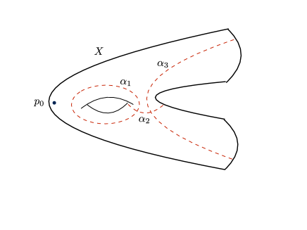
Figure 1.

The existence of such a system of curves and arcs is known; e. g., use Green lines on $X$ of Green’s function with pole at $p_{0}$ (cf. [21]). We denote by $\{q_{1},q_{2},\dots,q_{m}\}$ the set of all intersection points $\alpha_{i}\cap\alpha_{j}$ and $\alpha_{i}\cap\partial X$ $(i,j=1,2,\dots,k)$. Since $X^{\prime}$ is a simply connected Riemann surface, we have a Riemann map $\varphi:\Delta\to X^{\prime}$ with $\varphi(0)=p_{0}$. The map $\varphi$ can be continuously extended to $\partial\Delta$. Moreover, since $\partial X^{\prime}$ is piecewise analytic, $\varphi$ has an analytic continuation across $\partial\Delta$ except $\{\xi_{1},\xi_{2},\dots,\xi_{m^{\prime}}\}:=\cup_{i=1}^{m}\varphi^{-1}(q_{i})$, and $\varphi|\partial\Delta$ is a two to one map except for $\xi_{i}$ $(i=1,2,\dots,m^{\prime})$. We distinguish points on $\partial X^{\prime}$ according to images of $\varphi$. Namely, if $\partial X^{\prime}\ni q=\varphi(\xi_{1})=\varphi(\xi_{2})$ for $\xi_{1}\not=\xi_{2}$, we consider $q_{\xi_{i}}\in\partial X^{\prime}$ as $\lim_{\Delta\ni\lambda\to\xi_{i}}\varphi(\lambda)$ $(i=1,2)$ and they are different (Figure 2). Hence, $\varphi$ becomes a homeomorphism from $\overline{\Delta}$ onto $\overline{X^{\prime}}=X^{\prime}\cup\partial X^{\prime}$.

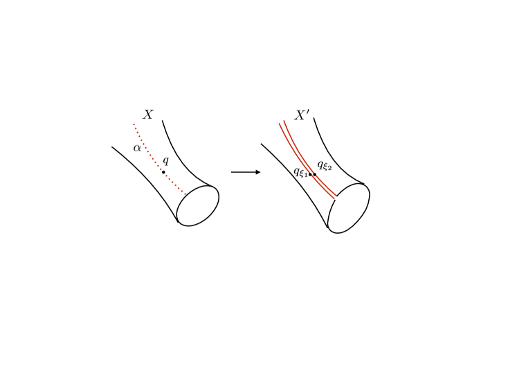
Figure 2.

Since the angle of $\partial X^{\prime}$ at each $q_{i}$ is $\pi/2$, we have

(6.1) $$|\varphi(\lambda)-\varphi(\xi_{j})|=O(|\lambda-\xi_{j}|^{1/2})\quad\textrm{as }\lambda\to\xi_{j}$$

for every $\xi_{j}\in\cup_{i=1}^{m}\varphi^{-1}(q_{i})$ and a local coordinate at $q_{i}$ $(i=1,2,\dots,m)$ (cf. [20]).

Step 2: Radial structures.

Let $\phi:\overline{X}\times(E\cup\overline{\Delta}_{r}\cup\Delta_{R}^{c})\to\widehat{\mathbb{C}}$ be a holomorphic motion of $E\cup\overline{\Delta}_{r}\cup\Delta_{R}^{c}$ over $\overline{X}$ as in Theorem 5.1. We consider a new holomorphic motion $\phi^{\prime}:\overline{X}\times(E\cup\{|z|\leq 2r\}\cup\{|z|\geq R-1\})\to\widehat{\mathbb{C}}$ by

$$\phi^{\prime}(p,z)=\begin{cases}\phi(p,z),&z\in E\\ z,&z\in\{|z|\leq 2r\}\cup\{|z|\geq R-1\}.\end{cases}$$

As the monodromy of $\phi$ is trivial, the monodromy of $\phi^{\prime}$ is also trivial; it follows from Proposition 4.1 that there exists a real analytic map $\Phi:\overline{X}\to M(\mathbb{C})$ such that ${\phi}_{0}:\overline{X}\times\widehat{\mathbb{C}}\to\widehat{\mathbb{C}}$ defined by

(6.2) $${\phi}_{0}(p,z)=w^{\Phi(p)}(z)$$

extends $\phi^{\prime}$. From Proposition 4.1 (2), $\phi_{0}(p,\cdot)$ is real analytic on $\{2r<|z|<R-1\}\setminus E$. Since $E$ is a finite set, $\phi_{0}(p,\cdot)$ is real analytic on $\{2r<|z|<R-1\}$. We may modify the map to have a smooth map on $\{r\leq|z|\leq R\}$ which extends $\phi_{0}$; we give a concrete construction of the extension.

For each $p\in\overline{X}$, we put $S_{p}=\{2r<|z|<R-1\}\setminus\{\phi(p.z_{1}),\dots,\phi(p,z_{n})\}$. The domain $S_{p}$ is a Riemann surface of type $(0;n,2)$ and a map $f_{p}:=\phi_{0}(p,\cdot)|S_{p_{0}}$ is a quasiconformal map from $S_{p_{0}}$ to $S_{p}$. From Proposition 3.4, there exists a real analytic symmetric quasiconformal map $e(f_{p}):S_{p_{0}}\cup\partial S_{p_{0}}\to S_{p}\cup\partial S_{p}$ which determines the same point in the reduced Teichmüller space $Teich^{\#}(S_{p_{0}})$ as $f_{p}$. In particular, $e(f_{p})(z)=\phi(p,z)$ for any $w\in E\cap S_{p_{0}}$. Furthermore, it follows from the symmetricity that $e(f_{p})(e^{i\theta}[2r,(R-1)])$ is orthogonal to $\{|z|=2r\}$ and $\{|z|=R-1\}$ for any $e^{i\theta}\in\partial\Delta$, where $e^{i\theta}[2r,(R-1)]$ is the closed line segment between $2re^{i\theta}$ and $(R-1)e^{i\theta}$. However, $e(f_{p})|\partial S_{p_{0}}$ may not be the identity. We extend the map to $\{R-1\leq|z|\}$ by the following way.

Put $e(f_{p})((R-1)e^{i\theta}))=(R-1)e^{i\Theta_{p}(\theta)}$ $(\Theta_{p}(\theta)\in[0,2\pi))$ for $\theta\in[0,2\pi)$. $\Theta_{p}$ is a homeomorphism from $[0,2\pi)$ onto $[\Theta_{p}(0),\Theta_{p}(0)+2\pi)$. We define a quadratic polynomial $g_{p}^{\theta}$ for each $\theta\in[0,2\pi)$ by

$$g_{p}^{\theta}(x)=A_{p}(x-\log(R-1))^{2}+\Theta_{p}(\theta),$$

where $A_{p}=(\theta-\Theta_{p}(\theta))(\log R-\log(R-1))^{-2}$; we see $g_{p}^{\theta}(\log(R-1))=\Theta_{p}(\theta)$, $(g_{p}^{\theta})^{\prime}(\log(R-1))=0$ and $g_{p}^{\theta}(\log R)=\theta$. Then, we define a map $\phi_{1}(p,w)$ for $(p,z)\in\overline{X}\times\{2r\leq|z|\}$ by

$$\phi_{1}(p,z)=\begin{cases}z,&(|z|>R)\\ e(f_{p})(z),&(2r\leq|z|<R-1)\\ |z|\exp\{ig_{p}^{\theta}(\log|z|)\},&(R-1\leq|z|\leq R,\arg z=\theta\in[0,2\pi)).\end{cases}$$

It is not hard to see that $g_{p}^{\theta}(x)\not=g_{p}^{\theta^{\prime}}(x)$ if $\theta\not=\theta^{\prime}$. Hence, the map $\phi_{1}$ is a diffeomorphism from $\overline{X}\times\{2r\leq|z|\leq R\}$ onto itself. In particular, $\phi_{1}(p,\cdot)$ is quasiconformal and $\phi_{1}(p,e^{i\theta}((R-1),R))$ is orthogonal to $\{|z|=R-1\}$ at $w=e(f_{p})((R-1)e^{i\theta})$.

Furthermore, there exist $\epsilon>0$ and $c>0$ such that for any $(p,\theta)\in\overline{X}\times[0,2\pi)$, the image of $\{z=\rho e^{i\theta}\mid R-c<\rho\leq R\}$ via $\phi_{1}(p,\cdot)$ is in the Stolz region at $Re^{i\theta}$ for $\epsilon$. Namely,

$$\frac{R-\rho}{|Re^{i\theta}-\phi_{1}(p,\rho e^{i\theta})|}>\epsilon$$

holds if $R-c<\rho\leq R$.

We may extend $\phi$ to $\overline{X}\times\{r\leq|z|\leq 2r\}$ by a similar way. We denote the extended map also by $\phi_{1}$. Then, at $re^{i\theta}$, $\phi_{1}(\{z=\rho e^{i\theta}\mid r\leq\rho<r+c\})$ is in the ”Stolz region” for some $\epsilon>0$;

$$\frac{\rho-r}{|re^{i\theta}-\phi_{1}(p,\rho e^{i\theta})|}>\epsilon$$

holds if $r\leq\rho<r+c$.

Thus, we have the map $\phi_{1}$ having the following properties:

1. $\phi_{1}:\overline{X}\times\widehat{\mathbb{C}}\to\widehat{\mathbb{C}}$ is a quasiconformal motion over $\overline{X}$, that is, a continuous family of quasiconformal maps parametrized by $\overline{X}$;

2. for each $p\in\overline{X}$ and $\zeta\in\partial\Delta_{R}$, $\phi_{1}(p,\zeta[r/R,1])$ is a differentiable arc, where $\zeta[a,b]$ $(0<a<b)$ is the closed line segment from $\zeta a$ to $\zeta b$;

3. $\phi_{1}(p,z)=\phi(p,z)$ for $(p,z)\in\overline{X}\times E$;

4. $\phi_{1}(p,z)=z$ if $z\in\Delta_{R}\setminus\overline{\Delta_{r}}$.

Naturally, the map $\phi_{1}$ is considered in $\overline{X^{\prime}}\times\widehat{\mathbb{C}}$. The set of simple arcs $\ell({\xi},{\zeta}):={\phi}_{1}(\xi,\zeta I)$ for $I=[0,1]\subset\mathbb{R}$ $(\xi\in\partial X^{\prime},\zeta\in\partial\Delta_{R})$ is called the “radial structure”in [25].

Lemma 6.1.

$\{\ell(\xi,\zeta)\mid\xi\in\partial X^{\prime},\zeta\in\partial\Delta_{R}\}$ has the following properties.

1. $\ell(\xi,\zeta)$ is a differentiable arc connecting $0$ and $\zeta$;

2. $\cup_{|\zeta|=R}\ell(\xi,\zeta)=\overline{\Delta}_{R}$ for each $\xi\in\partial X^{\prime}$;

3. $\ell(\xi,\zeta)\cap\ell(\xi,\zeta^{\prime})=\{0\}$ if $\zeta\not=\zeta^{\prime}$;

4. there exist $\zeta_{1},\dots,\zeta_{n}$ on $\partial\Delta_{R}$ such that $\phi(\xi,z_{i})\in\ell(\xi,\zeta_{i})$ $(i=1,\dots,n)$ for every $\xi\in\partial X^{\prime}$;

5. for any $\xi\in\partial X^{\prime}$, $\ell(\xi,\zeta)\cap\overline{\Delta}_{r}=\zeta[0,r]$, the line segment from $0$ to $r\zeta$;

6. Let $\xi^{\prime},\xi^{\prime\prime}$ be two distinct points on $\partial X^{\prime}$ corresponding to the same point $\xi$ in $X$. Then, $\ell(\xi^{\prime},\zeta)=\ell(\xi^{\prime\prime},\zeta)$ for any $\zeta\in\partial\Delta_{R}$;

7. there exist $\epsilon>0$ and $c>0$ such that the images of $\ell(\xi,\zeta)\cap\{|\zeta-z|<c\}$ and $\ell(\xi,\zeta)\cap\{|r\zeta/R-z|<c\}$ via $\phi_{1}(\xi,\cdot)$ are in the Stoltz regions at $\zeta$ and $r\zeta/R$ for $\epsilon$, respectively.

Proof.

Obvious are (2), (3) and (7) from the construction. The statement (5) is also easily verified because $\phi_{1}(\xi,z)=z$ if $z\in\Delta_{r}$.

Taking $\zeta_{i}=z_{i}R/|z_{i}|$ $(i=1,\dots,n)$, we see that $\phi(\xi,z_{i})={\phi}_{1}(\xi,z_{i})={\phi}_{1}(\xi,\zeta_{i}(|z_{i}|/R))\in\ell(\xi,\zeta_{i})$. Hence we have (4). Now, we show (1).

Since $\Phi:\overline{X}\to M(\mathbb{C})$ is real analytic, $\overline{X}\ni x\mapsto w^{\Phi(x)}(z)\in\widehat{\mathbb{C}}$ is real analytic on $\overline{X}$ for each $z\in\mathbb{C}$. We also see from Proposition 4.1 (2) that $\Phi(x)\in M(\mathbb{C})\subset L^{\infty}(\mathbb{C})$ is real analytic in $\mathbb{C}\setminus(E\cup\partial\Delta_{R})$. Therefore, $w^{\Phi(x)}(z)$ is real analytic with respect to $z$ in $\mathbb{C}\setminus(E\cup\partial\Delta_{R})$ (see [19]). Furthermore, $w^{\Phi(x)}$ is real analytic at every point of $E$ since $E$ is a finite set; we conclude that $w^{\Phi(x)}$ is real analytic except $\partial\Delta_{R}$. Thus, we have shown (1).

The statement (6) is trivial because $\phi_{1}(\xi^{\prime},\cdot)=\phi_{1}(\xi,\cdot)=\phi_{1}(\xi^{\prime\prime},\cdot)$.

∎

Step 3: A function space.

For a compact bordered Riemann surface $S$, let denote by $A_{S}$ the space of holomorphic functions on a some neighborhood $U$ of $\overline{S}$. We define $A(X^{\prime})$ by $A_{\Delta}\circ\varphi^{-1}$, where $\varphi$ is a Riemann map given in Step 1. Note that $X^{\prime}$ is simply connected and $X^{\prime}\cup\partial X^{\prime}$ is homeomorphic to $\overline{\Delta}$ via the Riemann map $\varphi:\Delta\to X^{\prime}$.

For each $\zeta\in\partial\Delta_{R}$, we define

(6.3) $$\mathcal{F}^{\zeta}=\{f\in A(X^{\prime})\mid f(\xi)\in\ell(\xi,\zeta)\textrm{ for every }\xi\in\partial X^{\prime}\},$$

and

(6.4) $$\mathcal{F}=\cup_{\zeta\in\partial\Delta_{R}}\mathcal{F}^{\zeta}.$$

Functions $f\equiv 0$, $\equiv\zeta$ and $\equiv r\zeta/|\zeta|$ are contained in $\mathcal{F}^{\zeta}$ for every $\zeta\in\partial\Delta_{R}$; it follows from Lemma 6.1 (4) that $\phi(\varphi(\cdot),\zeta_{i})\in\mathcal{F}^{\zeta_{i}}$ $(i=1,\dots,n)$.

We denote by $C^{\frac{1}{2}}(\partial\Delta)$ the space of complex valued Hölder continuous functions of exponent $\frac{1}{2}$, and by $C^{\frac{1}{2}}_{\mathbb{R}}(\partial\Delta)$ its subspace of all real valued functions.

One may find similar statement to the following lemma in [25] Lemma 1. 3; we give a different and an elementary proof.

Lemma 6.2.

$\mathcal{F}^{\zeta}\circ\varphi$ and $\mathcal{F}\circ\varphi$ are regarded as compact subsets of $C^{\frac{1}{2}}(\partial\Delta)$ by considering boundary values. Moreover, the followings hold:

1. If $g\in\mathcal{F}^{\zeta}$ and $\|g\|_{\infty}=R$, then $g(p)\equiv\zeta$;

2. if $g\in\mathcal{F}^{\zeta}$ and $|g(p)|\leq r$ for some $p\in\overline{X}$, then $g$ is a constant function.

Proof.

Since $f\in A(X^{\prime})$ is continuous on $X^{\prime}\cup\partial X^{\prime}$ and $\varphi:\Delta\cup\partial\Delta\to X\cup\partial X^{\prime}$ is a Höler continuous function of exponent $\frac{1}{2}$ by (6.1), we see that $f\circ\varphi\in A_{\Delta}$ belongs to $C^{\frac{1}{2}}(\partial\Delta)$. Thus, $\mathcal{F}^{\zeta}\circ\varphi$ and $\mathcal{F}\circ\varphi$ are in $C^{\frac{1}{2}}(\partial\Delta)$. The compactness of those spaces is easily verified.

Let $g\in\mathcal{F}^{\zeta}$ be a non-constant function with $\|g\|_{\infty}=R$. From (6.3) we see that $g\circ\varphi(\partial\Delta)\subset\cup_{\xi\in\partial X^{\prime}}\ell(\xi,\zeta)$ and $g\circ\varphi(\partial\Delta)\cap\partial\Delta_{R}=\{\zeta\}$. Hence, there exists $\lambda\in\partial\Delta$ such that $g(\varphi(\lambda))=\zeta$.

Now, we recall that $\ell(\xi,\zeta)$ is the image of the line segment $\zeta[0,1]$ via a quasiconformal map $\phi_{1}(\xi,\cdot)$ which keeps every point of $\partial\Delta_{R}$ fixed. From our construction of the radial structures, we see that the angle between $\ell(\xi,\zeta)$ and $\partial\Delta_{R}$ at $\zeta$ is greater than a positive constant $\epsilon$ which is independent of $\xi$ (Lemma 6.1 (7)). Therefore, the angle between $g(\partial X)\subset\cup_{\xi\in\partial X^{\prime}}\ell(\xi,\zeta)$ and $\partial\Delta_{R}$ at $\zeta$ is greater than $\epsilon>0$, and the angle of $g\circ\varphi(\partial\Delta)$ at $\zeta$ is less than $\pi-2\epsilon$. This means that the order of $g\circ\varphi$ at $\lambda$ is greater than one since $g\circ\varphi$ is holomorphic on $\partial\Delta$. Indeed, if the order is one, then $(g\circ\varphi)^{\prime}(\lambda)\not=0$ and $g\circ\varphi$ is conformal at $\lambda$; the angle of $g\circ\varphi(\partial\Delta)$ at $\lambda$ has to be $\pi$.

Thus, there exists a point $p^{\prime}\in X$ near $p=\varphi^{-1}(\lambda)$ such that $|g(p^{\prime})|>R$ and we have a contradiction. We complete the proof of (1).

To show (2), we first assume that there exists a non-constant function $g\in\mathcal{F}^{\zeta}$ such that it has a zero in $X^{\prime}$ but not on $\partial X^{\prime}$.

Since the monodromy of $\phi_{1}$ is trivial, we see that for every closed curve $\gamma$ in $\overline{X}$ and for every $x\in(0,\zeta)$, $\phi_{1}(\gamma,x)$ is freely homotopic to a trivial curve in $\widehat{\mathbb{C}}\setminus\{0,1,\infty\}$. In particular, the winding number of the curve $\phi_{1}(\partial X^{\prime},x)\subset\cup_{\xi\in\partial X^{\prime}}\ell(\xi,\zeta)$ around the origin is zero.

Let us consider the winding number of a closed curve $g(\partial X^{\prime})$ around the origin. Since the function $g$ belongs to $\mathcal{F}^{\zeta}$, both $g(\xi)$ and $\phi_{1}(\xi,x)$ are on the simple arc $\ell(\xi,\zeta)$ for every $\xi\in\partial X^{\prime}$. By moving $g(\xi)$ to $\phi_{1}(\xi,x)$ along $\ell(\xi,\zeta)$, we have a homotopy between $g(\partial X^{\prime})$ and $\phi_{1}(\partial X^{\prime},x)$. Since $\phi_{1}(\partial X^{\prime},x)$ does not pass the origin, we conclude that the winding number of $g(\partial X^{\prime})$ around the origin is also zero. Hence, the holomorphic function $g$ has a zero in $X^{\prime}$ by the argument principle and we have a contradiction.

Therefore, if $g\circ\varphi$ has zeros in $\overline{\Delta}$, then it has a zero on $\partial\Delta$. Noting that $\ell(\xi,\zeta)\cap\{|z|<r\}=\zeta[0,r/R)$ for every $\xi\in\partial X^{\prime}$ and $\zeta\in\partial\Delta_{R}$, we see that

$$g\circ\varphi(\partial\Delta)\cap\{|z|<r\}=\zeta[0,r/R].$$

Hence, the order of any zero of $g\circ\varphi$ on $\partial\Delta$ is even.

We note the following lemma:

Lemma 6.3.

Let $f$ be a holomorphic function in a neighborhood of an analytic closed curve $\gamma$. Suppose that the order of any zeros of $f$ on $\gamma$ is even and there exist a point $z_{0}\in\gamma$ and a neighborhood $U$ of $z_{0}$ such that $f(\gamma\cap U)\subset\mathbb{R}_{\geq 0}$. Then, $f(\gamma)\subset\mathbb{R}_{\geq 0}$.

Proof.

We may assume that $\gamma=\mathbb{R}$ and $z_{0}=0$. Let $I$ be the maximal interval on $\mathbb{R}$ containing $0$ such that $f(z)\geq 0$ for every $z\in I$. The interval $I$ is obviously a closed interval. Suppose that $I=[a,b]$ $(a<0<b)$. If $f(a)=0$, then we have

$$f(z)=c(z-a)^{2n}(1+\sum_{k=1}^{\infty}c_{k}(z-a)^{k})$$

near $z=a$ for some $n\in\mathbb{N}$ and a constant $c$. Since $f(x)>0$ for $x>a$ sufficiently close to $a$, we have $c>0$. Thus, we see that $f(x)>0$ for $x<a$ sufficiently close to $a$. It contradicts the maximality of $I$.

If $c_{0}:=f(a)>0$, then we have

$$f(z)=c_{0}+\sum_{k=1}^{\infty}c_{k}(z-a)^{k}$$

near $z=a$, say $(a-\epsilon,a+\epsilon)$ for some $\epsilon>0$. Since $f(x)>0$ for $a<x<a+\epsilon$, we see that $c_{1}=f^{\prime}(a)\in\mathbb{R}$. We also verify that $f^{\prime}(x)$ is real in $[a,a+\epsilon)$ because $f(x)$ is real there. Thus, $c_{2}=f^{\prime\prime}(a)/2$ is real. The same argument yields that $c_{k}$ is a real number for any $k\in\mathbb{N}$. Hence, $f$ is real valued in a neighborhood of $a$ on $\mathbb{R}$. From the continuity of $f$, we conclude that $f(x)>0$ near $x=a$. This contradicts the maximality of $I$.

The same argument works for $b$ and we conclude that $I=\gamma$. ∎

Applying Lemma 6.3 for $\gamma=\partial\Delta$ and $\zeta^{-1}(g\circ\varphi)$, we see that $\textrm{Im }\zeta^{-1}(g\circ\varphi)\equiv 0$ on $\partial\Delta$ and we have a contradiction. Thus $g\equiv 0$.

Next, we suppose that $0<\min\{|g(p)|\mid p\in\overline{X^{\prime}}\}<r$. Let $q_{0}$ be a point in $\overline{X^{\prime}}$ with $|g(q_{0})|=\min\{|g(p)|\mid p\in\overline{X^{\prime}}\}$. Applying the maximum principle to $g^{-1}$, we verify that $q_{0}$ is on $\partial X^{\prime}$. By the same argument as above, we see that the order of $g$ at $q_{0}$ is even. Hence, if $g$ is not a constant, then there exists a point $p^{\prime}\in X^{\prime}$ near $q_{0}$ such that $|g(p^{\prime})|<|g(q_{0})|$ and we have a contradiction.

Finally, we suppose that $\min\{|g(p)|\mid p\in\overline{X^{\prime}}\}=r$. Let $q_{0}\in\overline{X^{\prime}}$ be a point with $|g(q_{0})|=r$. By using the maximum principle again, we see that $q_{0}$ is on $\partial X^{\prime}$. Since $g\in\mathcal{F}^{\zeta}$, we have $g(q_{0})=r\zeta/|\zeta|$. We may use the same argument as in the proof of (1) for $g$ and for $\partial\Delta_{r}$. Then, we conclude that the angle between $g(\partial X^{\prime})$ and $\partial\Delta_{r}$ is strictly positive at $r\zeta/|\zeta|$ and the order of $g$ at $q_{0}$ is more that one. Hence, we see that there exists a point $p^{\prime}\in X^{\prime}$ near $q_{0}$ such that $|g(p^{\prime})|<r=|g(q_{0})|$. It is a contradiction and we complete the proof of (2). ∎

Step 4: Differential equations.

Since $X^{\prime}$ and $\partial X^{\prime}$ are identified with $\Delta$ and $\partial\Delta$, respectively, we may discuss our argument in $\Delta\cup\partial\Delta$ instead of $X^{\prime}\cup\partial X^{\prime}$. In this step, we will make our discussion in $\Delta\cup\partial\Delta$ for the sake of simplicity.

For any $(\xi,z)\in\partial\Delta\times\overline{\Delta_{R}}(\simeq\partial X^{\prime}\times\overline{\Delta_{R}})$, there exists a unique $\zeta\in\partial\Delta_{R}$ such that $\ell(\xi,\zeta)\ni z$. Since $\ell(\xi,\zeta)\cap(\overline{\Delta_{R}}\setminus\Delta_{r})$ is differentiable, we may consider the unit tangent vector of $\ell(\xi,\zeta)$ at $z\in\ell(\xi,\zeta)$ with $r\leq|z|\leq R$, where we parametrize the curve $\ell(\xi,\zeta)$ by the length parameter from $\zeta\in\partial\Delta_{R}$.

We denote by $\tau(\xi,z)$ the unit tangent vector of $\ell(\xi,\zeta)$ at $z\in\ell(\xi,\zeta)$. Hence, the parametrization $z(t)$ of $\ell(\xi,\zeta)$ satisfies a differential equation:

(6.5) $$\frac{d}{dt}z(t)=\tau(\xi,z(t)).$$

We see that there exists a differentiable map $\alpha:\partial\Delta\times(\overline{\Delta_{R}}\setminus\Delta_{r})\to\mathbb{R}$ such that

(6.6) $$\tau(\xi,z)=\frac{z}{|z|}e^{i\alpha(\xi,z)}.$$

Indeed, for every $\zeta\in\partial\Delta_{R}$, $\textrm{arg }\tau(\xi,\zeta)\zeta^{-1}$ is in $(-\pi/2.\pi/2)$. Thus, a map

$$\partial\Delta\times\partial\Delta_{R}\ni(\xi,\zeta)\mapsto\zeta^{-1}\tau(\xi,\zeta)/R\in\partial\Delta$$

is homotopic to a constant map. A continuity argument guarantees us the existence of the function $\alpha$. In fact, $\alpha$ is unique up to an additive constant $2n\pi$ $(n\in\mathbb{Z})$.

We may take $\delta>0$ so small that $\tau$ is extended to a differentiable map on $\partial\Delta\times(\Delta_{R+\delta}\setminus\Delta_{r})$. It is possible by our concrete construction of $\phi_{1}$ in Step 2.

We put

(6.7) $$\mathcal{U}:=\{g\in C^{\frac{1}{2}}(\partial\Delta)\cap A_{\Delta}\mid r<|g(\lambda)|<R+\delta\textrm{ for all $\lambda\in\overline{\Delta}$}\}.$$

$\mathcal{U}$ is an open subset of $C^{\frac{1}{2}}(\partial\Delta)\cap A_{\Delta}$.

Let $\beta(g)(\xi)=\alpha(\xi,g(\xi))$ for $\xi\in\partial\Delta$ and for $g\in\mathcal{U}$. Then we define a map

(6.8) $$F(g)=g\exp\{-T[\beta(g)]+iP[\beta(g)]\}$$

for $g\in\mathcal{U}$, where $P[f]$ is the Poisson integral of a real-valued continuous function $f$ on $\partial\Delta$ and $T[f]$ is the Hilbert transform of $f$, that is, $T[f](z)$ is the conjugate harmonic function of $P[f]$ with $T[f](0)=0$. Then, we show the following:

Lemma 6.4.

$F(\mathcal{U})\subset C^{\frac{1}{2}}(\partial\Delta)\cap A_{\Delta}$ and $F$ is locally Lipschitz on $\mathcal{U}$.

Proof.

Let $g\in\mathcal{U}$. Then, $F(g)$ gives a holomorphic function on $\Delta$. It follows from a property of the Hilbert transform that $F(g)$ belongs to $C^{\frac{1}{2}}(\partial\Delta)$ (cf. [7] Theorem 5.8). Hence, $F(\mathcal{U})\subset C^{\frac{1}{2}}(\partial\Delta)\cap A_{\Delta}$.

Since $\alpha$ is differentiable, so is $\beta$. Thus, a compactness argument shows that $F$ is locally Lipschitz on $\mathcal{U}$. ∎

Here, we consider a differential equation:

(6.9) $$\frac{dg_{t}}{dt}=F(g_{t}),\quad g_{t_{0}}=g_{0}\in\mathcal{U}.$$

By the standard fact on ordinary differential equations(cf. [5] Chapter X), we see that for any initial value $g_{t_{0}}\in\mathcal{U}$ the differential equation (6.9) has a unique solution $g_{t}\in\mathcal{U}$ in some interval $(a_{0},b_{0})$ with $a_{0}<t_{0}<b_{0}$.

If $g_{0}\in\mathcal{F}^{\zeta}$ for some $\zeta\in\partial\Delta_{R}$, then $g_{t}\in\mathcal{F}^{\zeta}$ as long as $r<\min_{\lambda\in\overline{\Delta}}|g_{t}(\lambda)|\leq\|g_{t}\|_{\infty}\leq R$. Indeed, from (6.8) and (6.9) we have for each $\xi\in\partial\Delta$

$$\frac{d}{dt}g_{t}(\xi) = F(g_{t}(\xi))=g_{t}(\xi)\exp\{-T(\beta(g_{t}(\xi)))+iP(\beta(g_{t}(\xi)))\}$$

$$= g_{t}(\xi)\exp\{-T(\alpha(\xi,g_{t}(\xi))+iP(\alpha(\xi,g_{t}(\xi)))\}$$

$$= \frac{g_{t}(\xi)}{|g_{t}(\xi)|}|F(g_{t}(\xi))|\exp\{iP(\alpha(\xi,g_{t}(\xi)))\}.$$

Noting that $P(f)(\xi)=f(\xi)$ for a continuous function $f$ on $\partial\Delta$, we obtain

$$\frac{d}{dt}g_{t}(\xi)=|F(g_{t}(\xi))|\tau(\xi,g_{t}(\xi)).$$

Therefore, for each $\xi\in\partial\Delta$, the function $u_{\xi}(t):=g_{t}(\xi)$ is a solution of

(6.10) $$\frac{d}{dt}u=|F(u)|\tau(\xi,u).$$

Comparing (6.5) and (6.10), we verify that $g_{t}(\xi)\in\ell(\xi,\zeta)$ if $g_{0}(\xi)\in\ell(\xi,\zeta)$ for $\xi\in\partial\Delta$. If $|g_{t}(\lambda)|\leq r$, then it follows from Lemma 6.2 (2) that $g_{t}$ is a constant function which does not belong to $\mathcal{U}$.

Let $\mathcal{I}$ be the largest interval where $g_{t}$ exists and belongs to $\mathcal{F}^{\zeta}\cap\mathcal{U}$. Then, $\mathcal{I}=(a,b]$ for some $a,b\in\mathbb{R}$. From the maximality of $\mathcal{I}$, we have

1. $g_{b}(\xi)=\zeta$ for every $\xi\in\partial\Delta$;

2. $\lim_{t\to\alpha+}g_{t}(\xi)=r\zeta/|\zeta|$ for every $\xi\in\partial\Delta$.

Thus, we verify that

(6.11) $$\textrm{the map }\mathcal{I}\ni t\mapsto g_{t}(\xi)\in\ell(\xi,\zeta)\cap(\overline{\Delta_{R}}\setminus\overline{\Delta_{r}})\textrm{ is a homeomorphism.}$$

Step 5: Extension.

Let $(\lambda,z)$ be in $\overline{\Delta}\times(\overline{\Delta_{R}}\setminus\overline{\Delta_{r}})$. Since $\cup_{\zeta\in\partial\Delta_{R}}\ell(\xi,\zeta)=\overline{\Delta_{R}}$ $(\xi\in\partial\Delta)$ and $\ell(\xi,\zeta)\cap\ell(\xi,\zeta^{\prime})=\{0\}$ if $\zeta\not=\zeta^{\prime}$, there exists a unique $\zeta\in\partial\Delta_{R}$ such that $z\in\ell(1,\zeta)$.

We consider the initial value problem of (6.9) for $g_{0}\equiv\zeta\in\mathcal{F}^{\zeta}\cap\mathcal{U}$. From the result in Step 4, $g_{t}$ belongs to $\mathcal{F}^{\zeta}$ for $t\in\mathcal{I}$ and there exists a unique $t({z})\in\mathcal{I}$ such that $g_{t({z})}(1)=z\in\ell(1,\zeta)\cap(\overline{\Delta_{R}}\setminus\overline{\Delta_{r}})$.

Thus, we have $g_{t(z)}\in\mathcal{F}^{\zeta}$ with $g_{t(z)}(1)=z$. If $g^{*}$ be a function of $\mathcal{F}^{\zeta}$ with $g^{*}(1)=z$, then we consider the initial value problem of (6.9) for $g_{t_{0}}=g^{*}$. Take the largest interval $\mathcal{I}^{*}=(\alpha^{*},\beta^{*}]$ for the problem as in Step 4. Then, $g^{*}_{\beta^{*}}\equiv\zeta$. From the uniqueness of the initial value problem, we verify that $g^{*}=g_{t(z)}$.

Therefore, we have the following.

Lemma 6.5.

For each $z\in\overline{\Delta_{R}}\setminus\overline{\Delta_{r}}$, there exists a unique $\zeta\in\partial\Delta_{R}$ and a unique $g:=g_{t(z)}\in\mathcal{F}^{\zeta}$ such that $g(1)=z$.

Let $z,z^{\prime}$ be two distinct points in $\overline{\Delta_{R}}\setminus\overline{\Delta_{r}}$. Then, there exist $\zeta,\zeta^{\prime}\in\partial\Delta$ such that $z\in\ell(1,\zeta)$ and $z^{\prime}\in\ell(1,\zeta^{\prime})$. Hence, $g_{t(z)}\in\mathcal{F}^{\zeta}$ and $g_{t(z^{\prime})}\in\mathcal{F}^{\zeta^{\prime}}$. We show that $g_{t(z)}(\xi)\not=g_{t(z^{\prime})}(\xi)$ for any $\xi\in\partial\Delta$.

From the definition of $\mathcal{F}$, $g_{t(z)}(\xi)\in\ell(\xi,\zeta)$ and $g_{t(z^{\prime})}(\xi)\in\ell(\xi,\zeta^{\prime})$. If $\zeta\not=\zeta^{\prime}$, then $g_{t(z)}(\xi)\not=g_{t(z^{\prime})}(\xi)$ for any $\xi\in\partial\Delta$ because $\ell(\xi,\zeta)\cap\ell(\xi,\zeta^{\prime})=\{0\}$ and $g_{t(z)}(\xi),g_{t(z^{\prime})}(\xi)\not=0$.

If $\zeta=\zeta^{\prime}$, then both $g_{t(z)}(\xi)$ and $g_{t(z^{\prime})}(\xi)$ are on the same curve $\ell(\xi,\zeta)$. However, $t(z)\not=t(z^{\prime})$. Thus, it follows from (6.11) that $g_{t(z)}(\xi)\not=g_{t(z^{\prime})}(\xi)$ for $\xi\in\partial\Delta$.

We put $G_{z,z^{\prime}}:=g_{t(z)}-g_{t(z^{\prime})}$. The above argument shows that $G_{z,z^{\prime}}$ is a non-vanishing continuous function on $\partial\Delta$ for each $(z,z^{\prime})\in(\overline{\Delta_{R}}\setminus\overline{\Delta_{r}})^{2}-\{\textrm{diagonals}\}$ and it is continuous with respect to $(z,z^{\prime})$. Hence, the winding number of $G_{z,z^{\prime}}(\partial\Delta)$ around the origin is independent of $(z,z^{\prime})$. From Lemma 6.2 (1), we have $g_{t(\zeta)}\equiv\zeta\in\partial\Delta_{R}$. Thus, we see that the winding number of $G_{\zeta,z^{\prime}}(\partial\Delta)=\zeta-g_{t(z^{\prime})}(\partial\Delta)$ around the origin has to be zero since $g_{t(z^{\prime})}(\Delta)\subset\Delta_{R}$ and $g_{t(z^{\prime})}(\partial\Delta)\not\ni\zeta$ if $z^{\prime}\in\Delta_{R}$. Obviously, the winding number of $G_{\zeta,z^{\prime}}(\partial\Delta)=\zeta-g_{t(z^{\prime})}(\partial\Delta)$ around the origin is zero when $z^{\prime}=\zeta^{\prime}(\not=\zeta)$ is on $\partial\Delta_{R}$. It follows from the argument principle that $g_{t(z)}-g_{t(z^{\prime})}$ does not have zeros in ${\Delta}$ if $z\not=z^{\prime}$. Therefore, the map

$$\overline{\Delta_{R}}\setminus\overline{\Delta_{r}}\ni z\mapsto g_{t(z)}(\lambda)\in\overline{\Delta_{R}}\setminus\overline{\Delta_{r}}$$

is injective and continuous for each $\lambda\in\overline{\Delta}$.

Now, we define a map $\Psi_{\lambda}:\widehat{\mathbb{C}}\to\widehat{\mathbb{C}}$ for each $\lambda\in\overline{\Delta}$ by

(6.12) $$\Psi_{\lambda}(z)=\begin{cases}g_{t(z)}(\lambda),\quad&z\in\overline{\Delta_{R}}\setminus\overline{\Delta_{r}}\\ z,\quad&\textrm{otherwise}.\end{cases}$$

As we have noted above, $\Psi_{\lambda}$ is a homeomorphism on $\widehat{\mathbb{C}}$ for each $\lambda\in\overline{\Delta}$; we define

(6.13) $$\widehat{\phi}(p,z)=\Psi_{\varphi^{-1}(p)}\circ\Psi_{0}^{-1}(z)$$

for $p\in\overline{X^{\prime}}$. We see that $\widehat{\phi}$ is a holomorphic motion of $\widehat{\mathbb{C}}$ over $\overline{X^{\prime}}$.

Indeed, for the basepoint $p_{0}\in X^{\prime}$, we have

$$\widehat{\phi}(p_{0},z)=\Psi_{0}(\Psi_{0}^{-1}(z))=z$$

as $\varphi^{-1}(p_{0})=0$. It is obvious that $\widehat{\phi}(p,\cdot)$ is a homeomorphism for each $p\in\overline{X^{\prime}}$.

If $z$ is in $\overline{\Delta_{R}}\setminus\overline{\Delta_{r}}$, then we have

$$\widehat{\phi}(p,z)=g_{t(z_{0})}(\varphi^{-1}(p)),$$

where $z_{0}$ is the point in $\overline{\Delta_{R}}\setminus{\overline{\Delta_{r}}}$ with $\Psi_{0}(z)=z_{0}$: $\hat{\phi}(p,z)$ is holomorphic with respect to $p\in\overline{X^{\prime}}$.

If $z$ is not in $\overline{\Delta_{R}}\setminus\overline{\Delta_{r}}$, then $\widehat{\phi}(p,z)=z$. Thus, we see that $\widehat{\phi}(\cdot,z)$ is holomorphic in $\overline{X^{\prime}}$ and we verify that $\widehat{\phi}$ is a holomorphic motion of $\widehat{\mathbb{C}}$ over $\overline{X^{\prime}}$.

Finally, we see that $\widehat{\phi}(p,\cdot)$ agrees with $\phi(p,\cdot)$ on $E=\{0,1,\infty,z_{1},z_{2},\dots,z_{n}\}$ for any $p\in X^{\prime}$. For $z_{j}\in E$ $(j=1,2,\dots,n)$, there exists $\zeta_{j}\in\partial\Delta_{R}$ such that $\phi(\varphi(\cdot),z_{j})\in\mathcal{F}^{\zeta_{j}}$ (see Lemma 6.1 (4)). In particular, $\omega_{j}:=\phi(\varphi(1),z_{j})$ is on $\ell(\varphi(1),\zeta_{j})$ by the definition of $\mathcal{F}^{\zeta_{j}}$, where $\varphi:\Delta\to X^{\prime}$ is the Riemann map given in Step 1. Since both $g_{t(\omega_{j})}$ and $\phi(\varphi(\cdot),z_{j})$ belong to $\mathcal{F}^{\zeta_{j}}$ and take the same value $\omega_{j}$ at $1$, it follows from the uniqueness of Lemma 6.5 that

$$\phi(\varphi(\cdot),z_{j})=g_{t(\omega_{j})}(\cdot)$$

on $\Delta$. Hence, we have

(6.14) $$\phi(\varphi(\lambda),z_{j})=g_{t(\omega_{j})}(\lambda)=\Psi_{\lambda}(\omega_{j})=\Psi_{\lambda}(\phi(1,z_{j}))$$

and

(6.15) $$\Psi_{0}(\phi(1,z_{j}))=\phi(p_{0},z_{j})=z_{j}.$$

Therefore, we conclude from (6.14) and (6.15) that

(6.16) $$\widehat{\phi}(p,z_{j})=\Psi_{\lambda}(\Psi_{0}^{-1}(z_{j}))=\Psi_{\lambda}(\phi(1,z_{j}))=\phi(p,z_{j}),\quad(\lambda=\varphi^{-1}(p))$$

for $p\in{X^{\prime}}$ $(j=1,2,\dots,n)$. That is, both holomorphic motions agree at $E$.

Step 6 : Getting a holomorphic motion over the whole Riemann surface $X$.

In Step 5, we obtain a holomorphic motion $\widehat{\phi}:\overline{X^{\prime}}\times\widehat{\mathbb{C}}\to\widehat{\mathbb{C}}$. Now, we show that $\widehat{\phi}$ becomes a holomorphic motion of $\widehat{\mathbb{C}}$ over $X$.

Let $\xi^{+},\xi^{-}$ be two points on $\partial X^{\prime}$ coming from the same point $\xi$ in $X$ (see Figure 2) and $z$ be a point in $\overline{\Delta}_{R}\setminus\overline{\Delta}_{r}$. There exists a unique $\zeta\in\partial\Delta_{R}$ such that $z$ is on $\ell(1,\zeta)$. We find a function $g_{t(z)}\in\mathcal{F}^{\zeta}$ appearing in (6.12) is the function in flow $\{g_{t}\}_{t\in\mathcal{I}}$ at time $t=t(z)$ such that $g_{t(z)}(1)=z$. It is obtained from the solution of the differential equation (6.9) for the initial value $g_{0}\equiv\zeta$.

We also see that $\mathcal{I}\ni t\mapsto g_{t}(\xi^{\pm})\in\ell(\xi^{\pm},\zeta)$ gives homeomorphisms of $\mathcal{I}$ onto $\ell(\xi^{\pm},\zeta)$ which are simple arcs from $\zeta$ to $r\zeta/|\zeta|$. On the other hand, from Lemma 6.1 (6), we have $\ell(\xi^{+},\zeta)=\ell(\xi^{-},\zeta)$ for any $\zeta\in\partial\Delta_{R}$. Hence, both $t\mapsto g_{t}(\xi^{+})$ and $t\mapsto g_{t}(\xi^{-})$ are solutions of the same differential equation with the same initial value $\zeta$. Thus, $g_{t}(\xi^{+})=g_{t}(\xi^{-})$ for every $t\in\mathcal{I}$. In particular, $g_{t(z)}(\xi^{+})=g_{t(z)}(\xi^{-})$. We verify that $g_{t(z)}(\xi):=g_{t(z)}(\xi^{\pm})$ is well defined; $\widehat{\phi}(\cdot,z)$ is a continuous function on $X$.

For each $z\in\widehat{\mathbb{C}}$, $X\ni p\mapsto\widehat{\phi}(p,z)$ is continuous on $X$ and holomorphic on $X^{\prime}=X\setminus\cup_{i=1}^{k}\alpha_{i}$. Since $\alpha_{i}$ $(i=1,2,\dots,k)$ are analytic curves, it follows from a fundamental result of complex analysis that $\widehat{\phi}(\cdot,z)$ must be a holomorphic function on $X$. Hence, we have obtained a desired holomorphic motion $\widehat{\phi}$ of $\widehat{\mathbb{C}}$ over $X$ which extends $\phi$. We have completed the proof of the theorem.

7. Proof of Theorem II

We prove both statements (1) and (2) by constructing examples.

Let $E$ be $\{0,1,\infty,z_{0},z_{1},\dots,z_{n}\}$. We consider a condition for the monodromy of a holomorphic motion of $E$ to be trivial.

Lemma 7.1.

Let $f$ be a holomorphic function on a Riemann surface $X$ with a basepoint $p_{0}$ such that $f(X)\cap(E\setminus\{z_{0}\})=\emptyset$ and $f(p_{0})=z_{0}$. Let $\phi_{f}$ be a holomorphic motion of $E$ over $X$ defined by

(7.1) $$\phi_{f}(p,z)=\begin{cases}z,\quad&(z\in E\setminus\{z_{0}\}),\\ f(p),\quad&(z=z_{0}).\end{cases}$$

Then, the monodromy of $\phi_{f}$ is trivial if and only if for any closed curve $\gamma$ in $X$,$f(\gamma)$ is homotopic to the trivial curve in $\mathbb{C}\setminus\{0,1,z_{1},\dots,z_{n}\}$.

Proof.

It is obvious that $\phi_{f}$ is a holomorphic motion of $E$ over $X$.

To consider the monodromy of $\phi_{f}$, we take a closed curve $\gamma$ on $X$ passing through $p_{0}$ and the lift $\tilde{\gamma}$ of $\gamma$ to the universal covering $\Delta$ of $X$. For the universal covering map $\pi:\Delta\to X$, $\tilde{\gamma}$ is a simple arc connecting two points $\zeta_{0},\zeta_{1}\in\pi^{-1}(p_{0})$.

By restricting the holomorphic motion $\tilde{\phi}_{f}(\cdot,z):=\phi_{f}(\pi(\cdot),z)$ $(z\in E)$ to a simply connected neighborhood $U$ of $\tilde{\gamma}$ in $\mathbb{H}$, we have a holomorphic motion $\tilde{\phi}_{f}|U$ of $E$ over $U$ with basepoint $\zeta_{0}$. Since $U$ is a simply connected domain which is conformally equivalent to the unit disk $\Delta$, it follows from Theorem 2.1 (2), $\tilde{\phi}_{f}|U$ is extended to a holomorphic motion, say $\hat{\phi}_{U}$, of $\widehat{\mathbb{C}}$ over $U$.

We have a continuous family $\{\varphi_{t}\}_{0\leq t\leq 1}$ by $\varphi_{t}(z)=\hat{\phi}_{U}(\tilde{\gamma}(t),z)$, where $\tilde{\gamma}(t)$ is a parametrization of $\tilde{\gamma}$ with $\tilde{\gamma}(0)=\zeta_{0}$ and $\tilde{\gamma}(1)=\zeta_{1}$. Moreover, each $\varphi_{t}$ is a quasiconformal self-map of $\widehat{\mathbb{C}}$ and $\varphi_{0}=id$. The map $\varphi_{1}$ determines the monodromy for $\gamma$.

Since $\varphi_{t}$ fixes each point of $E\setminus\{w_{0}\}$, $\{\varphi_{t}\}_{0\leq t\leq 1}$ gives a homotopy between $\varphi_{0}=id$ and $\varphi_{1}$. Therefore, $\varphi_{1}$ is homotopic to the identity in ${\mathbb{C}}\setminus\{0,1,z_{1}\dots,z_{n}\}$. Thus, it follows from [15] that $\varphi_{1}$ is homotopic to the identity on $\widehat{\mathbb{C}}\setminus E$ rel $E$ if and only if $\cup_{t\in[0,1]}\varphi_{t}(z_{0})=\phi(\pi(\tilde{\gamma}(t)),z_{0})=f(\gamma)$ is homotopic to the trivial curve. ∎

Proof of (1). We take closed curves $\gamma_{0},\gamma_{1}$ as in Figure 3 and put $\gamma=\gamma_{1}\gamma_{0}\gamma_{1}^{-1}\gamma_{0}^{-1}$. The curve $\gamma$ represents a non-trivial element of $\pi_{1}(\mathbb{C}\setminus\{0,1,z_{1},\dots,z_{n}\},z_{0})$.

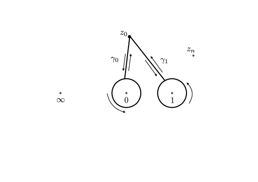
Figure 3.

For a parametrization $\gamma(t)$ $(0\leq t\leq 1)$ of $\gamma$ with $\gamma(0)=\gamma(1)=w_{0}$, we have

(7.2) $$\int_{\gamma}d\textrm{arg}(w-1)=\int_{\gamma}d\textrm{arg}w=0.$$

Let $\Gamma$ be a Fuchsian group acting on $\Delta$ such that $\Delta/\Gamma=\mathbb{C}\setminus\{0,1,z_{1},\dots,z_{n}\}$. Take $g\in\Gamma$ corresponding to $\gamma$. Then, $g$ is a hyperbolic Möbius transformation and $A:=\Delta/<g>=\{1<|\lambda|<R\}$ is an annulus for some $R>1$; we have a holomorphic covering map $\pi_{g}:A\to\mathbb{C}\setminus\{0,1,z_{1},\dots,z_{n}\}$. We take $\lambda_{0}\in A$ so that $\pi_{g}(\lambda_{0})=z_{0}$.

We take the point $\lambda_{0}\in A$ as a basepoint and define a map $\phi:A\times E\to\widehat{\mathbb{C}}$ by

(7.3) $$\phi(\lambda,z)=\begin{cases}z,\quad(z=0,1,\infty,z_{1},\dots,z_{n})\\ \pi_{g}(\lambda),\quad(z=z_{0}).\end{cases}$$

It is easy to see that $\phi$ is a holomorphic motion of $E$ over the Riemann surface $A$.

Consider $\alpha=\{|\lambda|=|\lambda_{0}|\}\subset A$. Then, $\phi(\alpha,z_{0})$ is a closed curve in $\mathbb{C}\setminus\{0,1\}$ homotopic to $\gamma$. It follows from (7.2) that

$$n(\alpha;z,z^{\prime})=0$$

for any distinct points $z,z^{\prime}$ in $E$.

Since the homotopy class of $\alpha$ generates $\pi_{1}(A,\lambda_{0})$, the holomorphic motion $\phi$ satisfies Chirka’s condition. However, Lemma 7.1 implies that the monodromy of $\phi$ is not trivial. Hence, the holomorphic motion $\phi$ cannot be extended to a holomorphic motion of $\widehat{\mathbb{C}}$ over $A$ and we obtain a desired example.

Proof of (2). The proof of (2) is done by using the same idea as in the proof of (1), but it is a bit complicated.

If the set $E$ consists of four points, then the above example constructed in (1) for $n=0$ is a desired one because any holomorphic motion of three points can be extended to a holomorphic motion of $\widehat{\mathbb{C}}$. Therefore, we may assume that $n\geq 1$.

For $E=\{0,1,\infty,z_{0},z_{1},\dots,z_{n}\}$, we take $\gamma_{0},\gamma_{1},\dots,\gamma_{n+1}$ in Figure 4. The homotopy classes of them are generators of a free group $F_{n+2}:=\pi_{1}(\widehat{\mathbb{C}}\setminus(E\setminus\{z_{0}\}),z_{0})$.

We put

$$\beta=\gamma_{0}\gamma_{1}\dots\gamma_{n+1}.$$

We define a sequence of closed curves, $\tilde{\gamma}_{1},\tilde{\gamma}_{2},\dots,\tilde{\gamma}_{n+1}$ by

(7.4) $$\tilde{\gamma}_{1}=[\gamma_{0},\gamma_{1}],\quad\mbox{and}\quad\tilde{\gamma}_{j}=[\gamma_{j},\tilde{\gamma}_{j-1}]\quad(j=2,\dots,n+1)$$

where $[a,b]=aba^{-1}b^{-1}$.

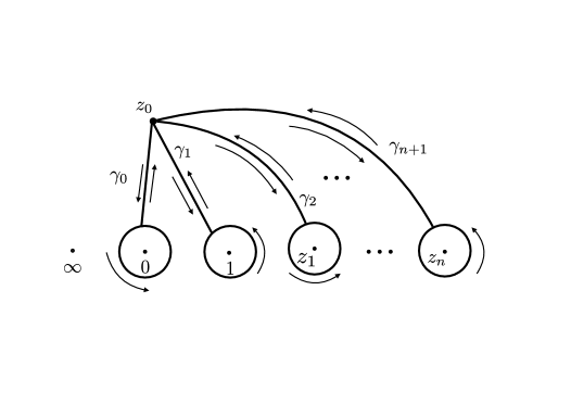
Figure 4.

Obviously, each of them represents a non-trivial element in $F_{n+2}$. Then, we put

(7.5) $$\gamma=[\beta,\tilde{\gamma}_{n+1}].$$

The curve $\gamma$ also represents a non-trivial element in $F_{n+2}$. Indeed, from the definition we have

$$\gamma = \beta\tilde{\gamma}_{n+1}\beta^{-1}\tilde{\gamma}_{n+1}^{-1}=\gamma_{0}\gamma_{1}\dots\gamma_{n+1}\tilde{\gamma}_{n+1}\gamma_{n+1}^{-1}\dots\gamma_{1}^{-1}\gamma_{0}^{-1}\tilde{\gamma}_{n+1}^{-1}$$

$$= \gamma_{0}\gamma_{1}\dots\gamma_{n+1}\gamma_{n+1}\tilde{\gamma}_{n}\gamma_{n+1}^{-1}\tilde{\gamma}_{n}^{-1}\gamma_{n+1}^{-1}\dots\gamma_{1}^{-1}\gamma_{0}^{-1}\tilde{\gamma}_{n}\gamma_{n+1}\tilde{\gamma}_{n}^{-1}\gamma_{n+1}^{-1}.$$

Since $\tilde{\gamma}_{n}=\gamma_{n}\tilde{\gamma}_{n-1}\gamma_{n}^{-1}\tilde{\gamma}_{n-1}^{-1}$, there is not a reduction in $\gamma_{0}^{-1}\tilde{\gamma}_{n}$ appearing at the last 3rd and 4th positions in the above word of $\gamma$. Hence, we verify that $\gamma$ represents a non-trivial element in $F_{n+2}$.

If we remove all $\gamma_{j}^{\pm}$ for the word of $\gamma$, then we have the trivial element since $\tilde{\gamma}_{j}$ becomes trivial and all of $\tilde{\gamma}_{i}$ $(i=j+1,\dots,n+1)$ become trivial. We see that $\gamma$ has the following property:

(A):

if we remove $\gamma_{j}^{\pm 1}$ from the word of $\gamma$ $(j=0,1,2,\dots$ or $n+1)$, then we obtain the trivial element.

Now, we consider a Fuchsian group $\Gamma_{n}$ acting on $\Delta$ such that $\Delta/\Gamma_{n}=\mathbb{C}\setminus\{0,1,z_{1},\dots,z_{n}\}$, which is isomorphic to $F_{n+2}$. Take $g\in\Gamma_{n}$ which corresponds to $\gamma$. The quotient space $\Delta/<g>$ is an annulus $A=\{1<|\lambda|<R\}$ for some $R>1$. We denote by $\pi_{g}:A\to\mathbb{C}\setminus\{0,1,z_{1},\dots,z_{n}\}$ the canonical projection and take $\lambda_{0}\in A$ with $\pi_{g}(\lambda_{0})=z_{0}$ as a basepoint. Take a circle $\alpha:=\{|\lambda|=|\lambda_{0}|\}\subset A$.

We define a holomorphic motion $\phi:A\times E\to\widehat{\mathbb{C}}$ over the Riemann surface $A$ by

$$\phi(\lambda,z)=\begin{cases}z,\quad&(z=0,1,z_{1},\dots,z_{n})\\ \pi_{g}(\lambda),\quad&(z=z_{0}).\end{cases}$$

Since the curve $\gamma$ represents a non-trivial element in $F_{n+2}$, we verify that the monodromy of $\phi$ for $\alpha$ is not trivial because of the same reason as in (1). Therefore, $\phi$ cannot be extended to a holomorphic motion of $\widehat{\mathbb{C}}$ over $A$.

Let $E^{\prime}$ be a proper subset of $E$. We see that $\phi|E^{\prime}$ is extended to a holomorphic motion of $E^{\prime}$ over $A$. It suffices to show that the monodromy of $\phi|{E^{\prime}}$ is trivial.

If $E^{\prime}$ does not contain $z_{0}$, then the monodromy of $\phi|{E^{\prime}}$ is trivial because $\phi(\lambda,z)=z$ for any $\lambda\in A$ and for any $z\in E^{\prime}$.

Suppose that $E^{\prime}$ contains $z_{0}$. Since $E^{\prime}$ consists of at most $(n+3)$ points containing $z_{0}$, it does not contain at least one point in $\{0,1,\infty,z_{1},\dots,z_{n}\}$.

If $E^{\prime}\not\ni\infty$, then the curve $\beta$ is trivial because it surrounds $\infty$. Hence, $\gamma(=[\beta,\tilde{\gamma}_{n+1}])$ represents the trivial element of $\pi_{1}(\widehat{\mathbb{C}}\setminus(E^{\prime}\setminus\{z_{0}\}),z_{0})$.

If $E^{\prime}\not\ni z\in\{0,1,z_{1},\dots,z_{n+1}\}$, then some $\gamma_{j}$ surrounding $z$ becomes trivial. Hence, from the property (A), we verify that the curve $\gamma$ also represents the trivial element of $\pi_{1}(\widehat{\mathbb{C}}\setminus(E^{\prime}\setminus\{z_{0}\}),z_{0})$.

Thus, in any case, we see that $\gamma$ represents the trivial element of $\pi_{1}(\widehat{\mathbb{C}}\setminus(E^{\prime}\setminus\{z_{0}\}),z_{0})$; a closed curve $\gamma_{\alpha}:=\phi(\alpha,z_{0})$ is homotopic to the trivial curve in $\pi_{1}(\widehat{\mathbb{C}}\setminus(E^{\prime}\setminus\{z_{0}\}),z_{0})$ since $\gamma_{\alpha}$ is homotopic to $\gamma$ from the construction of the Riemann surface $A$. From Lemma 7.1, we verify that the monodromy of $\phi|E^{\prime}$ is trivial for any $E^{\prime}$.

8. Proof of Theorem III

We may obtain Theorem III from Theorem I. It is done by following the argument of Earle-Kra-Krushkal [8]. For readers’ convenience, we will give a sketch of the proof.

Let $G$ be a subgroup of $\textrm{M\"{o}b}(\mathbb{C})$ and $E$ be a $G$-invariant subgroup of $\widehat{\mathbb{C}}$. As in Theorem I, we to show that if the monodromy of a $G$-equivariant holomorphic motion $\phi$ of $E$ over $X$ is trivial, then it is extended to a $G$-equivariant holomorphic motion of $\widehat{\mathbb{C}}$ over $X$.

For simplicity, we assume that $G$ is torsion free. First of all, we may assume that $E$ is a closed subset of $\widehat{\mathbb{C}}$ because of the $\lambda$-lemma. Hence, $E$ contains the set of all fixed points of $G$ since a fixed point of any $g\in G$ is either an attracting or a repelling fixed point of $g$.

Let $\phi:X\times E\to\widehat{\mathbb{C}}$ be a $G$-equivariant holomorphic motion of $E$ over $X$ satisfying (2.2). Then, since $\{\theta_{p}\}_{p\in X}$ is a holomorphic family of isomorphisms of $G$ obtained by quasiconformal maps, every $\theta_{p}$ is a type-preserving isomorphism.

Take a point $z_{0}$ in $E^{c}$. Then, there exists a holomorphic motion $\phi_{0}:X\times(E\cup\{z_{0}\})\to\widehat{\mathbb{C}}$ which extends $\phi$. Indeed, it follows from Theorem I that we have a holomorphic motion of $\widehat{\mathbb{C}}$ over $X$ which extends $\phi$. By restricting the holomorphic motion to $E\cup\{z_{0}\}$, we have the desired holomorphic motion $\phi_{0}$.

Now, we define a map $\widehat{\phi}_{0}$ on $X\times(E\cup G(z_{0}))$ by

(8.1) $$\widehat{\phi}_{0}(p,z)=\begin{cases}\phi_{0}(p,z),\quad z\in E\cup\{z_{0}\}\\ \theta_{p}(g)(\phi_{0}(p,z_{0})),\quad z=g(z_{0}).\end{cases}$$

We will show that $\widehat{\phi}_{0}$ is a $G$-equivariant holomorphic motion of $E\cup G(z_{0})$.

Since $\theta_{p_{o}}(g)=g$ for $g\in G$, we have $\widehat{\phi}_{0}(p_{0},\cdot)=id$ on $E\cup G(z_{0})$. It is also obvious that $\widehat{\phi}_{0}(\cdot,z)$ is holomorphic on $X$. We show the injectivity of $\widehat{\phi}_{0}(p,\cdot)$.

From the $G$-invariance of $E$, we see that $E\cap G(z_{0})=\emptyset$ and $\widehat{\phi}_{0}(p,\cdot)$ is injective on $E$. Suppose that $\widehat{\phi}_{0}(p,z)=\widehat{\phi}_{0}(p,g(z_{0})$ for some $z\in E$ and $g\in G$. Then we have

(8.2) $$\phi_{0}(p,z)=\theta_{p}(g)(\phi_{0}(p,z_{0})).$$

However, from the $G$-invariance of $E$ we have

$$\phi_{0}(p,E)=\phi_{0}(p,G(E))=\theta_{p}(G)(\phi_{0}(p,E)).$$

Hence, $\phi_{0}(p,E)$ is $\theta(G)$ invariant. Since $\phi_{0}(p,z_{0})$ is not in $\phi_{0}(p,E)$, it contradicts (8.2).

Finally, suppose that $\widehat{\phi}_{0}(p,g_{1}(z_{0}))=\widehat{\phi}_{0}(p,g_{2}(z_{0}))$ for $g_{1},g_{2}\in G$. Then, we have

$$\theta_{p}(g_{1})(\phi_{0}(p,z_{0}))=\theta_{p}(g_{2})(\phi_{0}(p,z_{0})).$$

If $g_{1}\not=g_{2}$, then $\phi_{0}(p,z_{0})$ is a fixed point of $\theta_{p}(g_{1}^{-1}\circ g_{2})$. However, this implies that $\phi_{0}(p,z_{0})$ is contained in $\phi_{0}(p,E)$ which is $\phi(p,E)$, and we have a contradiction since $\phi_{0}(p,\cdot)$ is injective on $E\cup\{z_{0}\}$. Thus, we have shown that $\widehat{\phi}_{0}$ is a holomorphic motion of $E\cup G(z_{0})$. The $G$-equivariance of $\widehat{\phi}_{0}$ is trivial from (8.1).

By repeating this procedure, we obtain a $G$-equivariant holomorphic motion $\widehat{\phi}_{\infty}$ of a countable dense subset $E_{\infty}$ of $\widehat{\mathbb{C}}$ over $X$. It follows from the $\lambda$-lemma that $\widehat{\phi}_{\infty}$ is extended to a holomorphic motion of $\widehat{\mathbb{C}}$, the closure of $E_{\infty}$. It is also easy to verify that the extended holomorphic motion is $G$-equivariant. Thus, we have completed the proof of Theorem III.

9. Applications.

9.1. Topological conditions for the extendability of holomorphic motions

A map $\phi:M\times E\to\widehat{\mathbb{C}}$ is called a continuous motion of $E$ over $M$ if it satisfies the conditions (1), (2) in Definition 2.1 and

(3’) $\phi$ is continuous in $M\times E$ and for each $p\in M$, $\phi(p,\cdot)$ is a homeomorphism from $E$ onto its image.

The concept of the monodromy of holomorphic motions is topological. Hence, immediately we have the following.

Theorem IV.

Let $\phi:X\times E\to\widehat{\mathbb{C}}$ be a holomorphic motion of $E$ over a Riemann surface $X$. Suppose that $\phi$ is extended to a continuous motion of $\widehat{\mathbb{C}}$ over $X$. Then,

1. the holomorphic motion $\phi$ is extended to a holomorphic motion of $\widehat{\mathbb{C}}$ over $X$;

2. if $\phi$ is $G$-equivariant for a subgroup $G$ of $\textrm{M\"{o}b}(\mathbb{C})$, then it is extended to a $G$-equivariant holomorphic motion of $\widehat{\mathbb{C}}$ over $X$.

Remark 9.1.

1. In the second statement, we do not assume that the extended continuous motion is $G$-equivariant.

2. Gardiner, Jiang and Wang [11] announce that if a holomorphic motion $\phi:X\times E\to\widehat{\mathbb{C}}$ has a guiding quasiconformal isotopy, then $\phi$ is extended to a holomorphic motion of $\widehat{\mathbb{C}}$ over $X$ which extends $\phi$. A guiding isotopy is a continuous motion with a quasiconformal nature (see [11] for the precise definition). Hence, Theorem IV confirms their result.

Now, we consider the triviality of the monodromy. In general, it is not easy to see if the monodromy of a holomorphic motion is trivial or not. However, under a certain condition the monodromy becomes automatically trivial (cf. [2] Lemma 8.1).

Proposition 9.1.

Let $E\subset\widehat{\mathbb{C}}$ be a closed set and $w:\widehat{\mathbb{C}}\to\widehat{\mathbb{C}}$ be a quasiconformal homeomorphism fixing each point of $E$. Suppose that $E$ is connected. Then, $w$ is homotopic to the identity rel $E$.

A discrete subgroup of $\textrm{M\"{o}b}(\mathbb{C})$ is called a Kleinian group. The limit set $\Lambda(G)$ of a Kleinian group $G$ is defined by the closure of the set of fixed points of elements of $G$ with infinite order. The limit set $\Lambda(G)$ of $G$ is closed and invariant under the action of $G$. A Kleinian group $G$ is called non-elementary if the limit set $\Lambda(G)$ contains more than two points.

From Theorems I, III and Proposition 9.1, immediately we have

Corollary 9.1.

Let $\phi:X\times E\to\widehat{\mathbb{C}}$ be a holomorphic motion of $E$ over a Riemann surface $X$. Suppose that $E$ is connected. Then, $\phi$ can be extended to a holomorphic motion of $\widehat{\mathbb{C}}$ over $X$.

Furthermore, if the holomorphic motion $\phi$ is $G$-equivariant for a subgroup $G$ of $\textrm{M\"{o}b}(\mathbb{C})$, then the holomorphic motion can be extended to a $G$-equivariant holomorphic motion of $\widehat{\mathbb{C}}$ over $X$.

Remark 9.2.

If the limit set $\Lambda(G)$ of a non-elementary Kleinian group $G$ is not connected, then there is a $G$-equivariant holomorphic motion of $\Lambda(G)$ over the punctured disk $\Delta^{*}:=\{0<|z|<1\}$ which cannot be extended to a holomorphic motion of $\widehat{\mathbb{C}}$ over $\Delta^{*}$ ([23] Theorem II).

9.2. A geometric condition for the extendability of holomorphic motions

Let $E=\{0,1,\infty,z_{1},\dots,z_{n}\}$ be a finite subset of $(n+3)$ points in $\widehat{\mathbb{C}}$. On the Riemann surface $S_{E}:=\widehat{\mathbb{C}}\setminus E$, we may define the hyperbolic metric which is the projection of the hyperbolic metric ${(1-|z|^{2})^{-1}}|dz|$ of the unit disk, the universal covering of $S_{E}$.

For the set $E$, we consider the following quantity:

(9.1) $$L(E)=\min\left\{\log(2+\sqrt{5}),\frac{1}{2}\log\left(\left(\frac{\ell(E)}{\pi}\right)^{2}+1\right)\right\},$$

where $\ell(E)$ is the minimal length of non-trivial and non-peripheral closed curves in $S_{E}$ with respect to the hyperbolic metric on $S_{E}$. Then, we have the following.

Theorem V.

Let $X$ be a hyperbolic Riemann surface with a basepoint $p_{0}$. Suppose that the fundamental group $\pi_{1}(X,p_{0})$ is of finitely generated and there exist closed curves $\gamma_{1},\gamma_{2},\dots,\gamma_{m}$ passing though $p_{0}$ such that the homotopy classes of those curves generate $\pi_{1}(X,p_{0})$ and

(9.2) $$\ell(\gamma_{j})<L(E)\quad(j=1,2,\dots,m)$$

hold, where $\ell(\gamma)$ is the hyperbolic length of a curve $\gamma\subset X$. Then, every holomorphic motion $\phi:X\times E\to\widehat{\mathbb{C}}$ of $E$ over $X$ can be extended to a holomorphic motion of $\widehat{\mathbb{C}}$ over $E$.

Proof.

Let $\phi:X\times E\to\widehat{\mathbb{C}}$ be a holomorphic motion of $E$ over a Riemann surface $X$ satisfying (9.2). From Theorem I, it suffices to show that the monodromy of $\phi$ is trivial. Since the triviality of the monodromy is the triviality of a homomorphism from $\pi_{1}(X,p_{0})$ to $\textrm{Mod}(0,n+3)$, it is enough to show that each $\gamma_{j}$ $(j=1,2,\dots,m)$ gives the identity of $\textrm{Mod}(0,n+3)$. To show it, we consider the action of the pure mapping class group, which is a subgroup of $\textrm{Mod}(0,n+3)$, on the Teichmüller space $Teich(S_{E})$.

Let $P\textrm{Mod}(0,n+3)$ denote a subgroup of mapping classes in $\textrm{Mod}(0,n+3)$ whose representatives are quasiconformal maps of $\widehat{\mathbb{C}}$ fixing each point of $E$. The subgroup $P\textrm{Mod}(0,n+3)$ is called the pure mapping class group. We consider the infimum of translation lengths of $P\textrm{Mod}(0,n+3)$ of $P_{0}:=[S_{E},id]\in Teich(S_{E})$. That is,

(9.3) $$r_{E}=\inf\{d_{T}(P_{0},\chi(P_{0})):\chi\in P\textrm{Mod}(0,n+3)\setminus\{id\}\},$$

where $d_{T}$ is the Teichmüller distance defined in §2. Then, we have shown the following.

Proposition 9.2 ( ([22] Theorem 2.1) ).

$$L(E)\leq r_{E}.$$

Let $\Gamma$ be a Fuchsian group on $\Delta$ which represents $X$. For the natural projection $\pi:\Delta\to\Delta/\Gamma=X$, the map $\tilde{\phi}(\lambda,z):=\phi(\pi(\lambda),z)$ $(\lambda\in\Delta,z\in E)$ defines a holomorphic motion of $E$ over $\Delta$. We see from Proposition 3.2 that there exists a holomorphic map $\Phi:\Delta\to Teich(S_{E})$ such that $\Phi(\lambda)$ gives $\widehat{\mathbb{C}}\setminus\tilde{\phi}(\pi(\lambda),E)$ as a point in $Teich(S_{E})$ for any $\lambda\in\Delta$.

We may take $0\in\Delta$ so that $\pi(0)=p_{0}\in X$. Then, we have $\Phi(0)=P_{0}$. Let $\tilde{\gamma}_{j}$ be a lift of $\gamma_{j}$ on $\Delta$ which begins at $0$ $(j=1,2,\dots,m)$. Then, there exists $g_{j}\in\Gamma$ such that $g_{j}(0)$ is the end point of $\tilde{\gamma}_{j}$. Since $\pi(g_{j}(0))=\pi(0)=p_{0}$, we have $\tilde{\phi}(g_{j}(0),z)=\tilde{\phi}(0,z)=z$ for any $z\in E$. Hence, there exists $\chi_{j}\in P\textrm{Mod}(0,n+3)$ such that

$$\Phi(g_{j}(0))=\chi_{j}(\Phi(0))=\chi_{j}(P_{0}).$$

The Teichmüller distance is the Kobayashi distance. It follows from the distance decreasing property of the Kobayashi distance (cf. [14]) that

(9.4) $$d_{T}(P_{0},\chi_{j}(P_{0}))=d_{T}(\Phi(0),\Phi(g_{j}(0)))\leq d_{\Delta}(0,g_{j}(0)),$$

where $d_{\Delta}$ is the hyperbolic distance in $\Delta$, which is the Kobayashi distance of $\Delta$.

On the other hand, since $\tilde{\gamma}_{j}$ is an arc from $0$ to $g_{j}(0)$, we have

(9.5) $$\ell(\gamma_{j})\geq d_{\Delta}(0,g_{j}(0)).$$

Combining (9.2), (9.4), (9.5) and Proposition 9.2, we have

$$d_{T}(P_{0},\chi_{j}(P_{0}))\leq\ell(\gamma_{j})<L(E)\leq r_{E}$$

for each $j$ $(1\leq j\leq m)$. Therefore, we conclude that $\chi_{j}=id$ for every $j$ $(j=1,2,\dots,m)$ because of (9.3). Thus, we have proved that the monodromy of the holomorphic motion $\phi$ is trivial.

∎

Let $A$ be an annulus $\{1<|\lambda|<R\}$ $(R>1)$. Then, the curve $\alpha:=\{|\lambda|=\sqrt{R}\}$ is the shortest closed curve with respect to the hyperbolic metric on $A$ which generates the fundamental group of $A$. It is not hard to see that the hyperbolic length of $\alpha$ is $\pi^{2}/\log R$. Hence, from Theorem V we have the following.

Corollary 9.2.

Let $E$ be a finite set in $\widehat{\mathbb{C}}$ and $A=\{1<|\lambda|<R\}$ be an annulus with a basepoint $p_{0}=\sqrt{R}$. Suppose that

$$R>\exp\left\{\frac{\pi^{2}}{L(E)}\right\}.$$

Then, any holomorphic motion of $E$ over $A$ is extended to a holomorphic motion of $\widehat{\mathbb{C}}$ over $A$.

9.3. Lifting problems

As we have seen in §3.1, there is a surjective map from the space of Beltrami coefficients to the Teichmüller space. The Douady-Earle section in §3.2 gives the inverse map of the surjective map; however, the section is not holomorphic.

It is known that there exists no holomorphic inverses on the Teichmüller space. We show that any holomorphic map from a Riemann surface to the Teichmüller space can be lifted to a holomorphic map to the space of Beltrami coefficients. We consider the problem for two kinds of Teichmüller spaces, Teichmüller space of a Riemann surface and that of a closed set, separately.

Teichmüller space of a Riemann surface. Let $S$ be a hyperbolic Riemann surface represented by a Fuchsian group $\Gamma$ on $\Delta$. Let $\pi_{\Gamma}:\textrm{Belt}(\Gamma)\to Teich(S)$ be the holomorphic projection defined in §3.1. Then, we have the following.

Theorem VI.

Let $F:X\to Teich(S)$ be a holomorphic map from a Riemann surface $X$ to the Teichmüller space $Teich(S)$ of a Riemann surface $S$ represented by a Fuchsian group $\Gamma$ on $\Delta$. Then, there exists a holomorphic map $\tilde{F}$ from $X$ to $\textrm{Belt}(\Gamma)$ which satisfies the following commutative diagram.

Proof.

To prove the theorem, we introduce the Bers embedding of $Teich(S)$ (cf. [12]).

For each $\mu\in\textrm{Belt}(\Gamma)$, we put

(9.6) $$\tilde{\mu}(z)=\begin{cases}\mu(z),\quad&(z\in\Delta)\\ 0,\quad&(z\in\Delta^{c}).\end{cases}$$

Then, the function $\tilde{\mu}$ belongs to $M(\mathbb{C})$, the space of Beltrami coefficients on $\mathbb{C}$. Moreover, it is $\Gamma$-compatible, namely, it satisfies

$$\tilde{\mu}(\gamma(z))\frac{\overline{\gamma^{\prime}(z)}}{\gamma^{\prime}(z)}=\tilde{\mu}(z)$$

almost everywhere in $\mathbb{C}$.

We take a quasiconformal map $f^{\mu}$ on $\widehat{\mathbb{C}}$ for $\tilde{\mu}$. The map is a solution of the Beltrami equation

$$\overline{\partial}f=\tilde{\mu}\partial f$$

in $\mathbb{C}$. From the definition (9.6), the map $f^{\mu}$ is conformal in ${\overline{\Delta}}^{c}$. We normalize $f^{\mu}$ by

$$f^{\mu}(z)=z+O\left(\frac{1}{z}\right)$$

as $z\to\infty$. We see that $f^{\mu}$ is uniquely determined by $\mu$.

Since $\tilde{\mu}$ is $\Gamma$-compatible, there exists an isomorphism $\Theta_{\mu}:\Gamma\to\textrm{M\"{o}b}(\mathbb{C})$ such that

(9.7) $$f^{\mu}(\gamma(z))=\Theta_{\mu}(\gamma)(f^{\mu}(z))$$

holds for every $\gamma\in\Gamma$ and for every $z\in\mathbb{C}$. It is known that $f^{\mu}$ and the isomorphism $\Theta_{\mu}$ depend only on $[\mu]_{\Gamma}\in Teich(S)$. Therefore, we may denote them by $f^{[\mu]_{\Gamma}}$ and $\Theta_{[\mu]_{\Gamma}}$, respectively. The group $\Gamma_{[\mu]_{\Gamma}}:=\Theta_{[\mu_{\Gamma}]}(\Gamma)$ is a quasiconformal conjugate to $\Gamma$ called a quasi-Fuchsian group and its limit set $\Lambda(\Gamma_{[\mu]_{\Gamma}})$ is a Jordan curve.

Taking the Schwarzian derivative $\{f^{[\mu]_{\Gamma}},\cdot\}$ of $f^{[\mu]_{\Gamma}}$ in ${\overline{\Delta}}^{c}$, we have from (9.7)

$$\{f^{[\mu]_{\Gamma}},\gamma(z)\}\gamma^{\prime}(z)^{2}=\{f^{[\mu]_{\Gamma}},z\}\quad(z\in{\overline{\Delta}}^{c}).$$

The above equation shows that the Schwarzian derivative $\{f^{[\mu]_{\Gamma}},\cdot\}$ is a holomorphic quadratic differential for $\Gamma$; it is bounded, i. e.,

$$\sup_{z\in{\overline{\Delta}}^{c}}\rho_{{\overline{\Delta}}^{c}}^{-2}|\{f^{[\mu]_{\Gamma}},z\}|<+\infty,$$

where $\rho_{{\overline{\Delta}}^{c}}(z)|dz|$ is the Poincaré metric on ${\overline{\Delta}}^{c}$. Since the Schwarzian derivative depends only on $[\mu]_{\Gamma}(=\pi_{\Gamma}(\mu))$, we may denote it by $\beta([\mu]_{\Gamma})$.

Thus, we have a map $\beta$ on the Teichmüller space $Teich(S)$ of $S$ to the space of bounded holomorphic quadratic differentials on ${\overline{\Delta}}^{c}$ for $\Gamma$. It is known that the map $\beta$ is injective and holomorphic on $Teich(S)$ and it is called the Bers embedding of $Teich(S)$.

Now, we consider a holomorphic map $\Phi:=\beta\circ F$ on $X$. Then, the conformal maps $f^{\Phi(\lambda)}$ $(\lambda\in X)$, which are solutions of $\{f,z\}=\Phi(\lambda)(z)$ on ${\overline{\Delta}}^{c}$, depend holomorphically on $\lambda\in X$. Therefore, we have a holomorphic motion $\phi$ of ${\overline{\Delta}}^{c}$ over $X$ defined by

(9.8) $$\phi(\lambda,z)=f^{\Phi(\lambda)}(z),\quad(\lambda,z)\in X\times{\overline{\Delta}}^{c}.$$

It follows from the $\lambda$-lemma that the holomorphic motion is extended to a holomorphic motion of $\Delta^{c}$ over $X$. The extended holomorphic motion is $\Gamma$-equivariant because of (9.7). Since $\Delta^{c}$ is connected, there exists a $\Gamma$-equivariant holomorphic motion $\widehat{\phi}$ of $\widehat{\mathbb{C}}$ over $X$ which extends $\phi$ by Corollary 9.1. Define

$$\widetilde{F}(\lambda)=\frac{\overline{\partial}\widehat{\phi}(\lambda,\cdot)}{\partial\widehat{\phi}(\lambda,\cdot)}\in\textrm{Belt}(\Gamma),\quad(\lambda\in X)$$

then it is a lift of $F$ from the construction. Furthermore, it is holomorphic by Theorem 2 in [8]; we obtain a holomorphic lift $\widetilde{F}$ of $F$ as desired.

∎

Teichmüller space of a closed set. Let $E$ be a closed set in $\widehat{\mathbb{C}}$. We consider the lifting problem for $T(E)$. First, we note a relationship between a holomorphic maps $F:X\to T(E)$ and holomorphic motions with trivial monodromy.

Let $\phi:X\times E\to\widehat{\mathbb{C}}$ be a normalized holomorphic motion of $E$ over a Riemann surface $X$. We may assume that the universal covering $\widetilde{X}$ of $X$ is conformally equivalent to the unit disk $\Delta$ unless the holomorphic motion is trivial.

Indeed, if $\widetilde{X}$ is conformally equivalent to the Riemann sphere or the complex plane, then $\widetilde{X}$ does not admit a non-constant bounded holomorphic function on $\widetilde{X}$. It follows from Theorem 1 in [18] that $\phi\circ\pi$ is a trivial holomorphic motion of $E$ over $\widetilde{X}$, where $\pi:\widetilde{X}\to X$ is a universal covering map and $\phi\circ\pi$ is a holomorphic motion of $E$ over $\widetilde{X}$ defined by $\phi\circ\pi(p,z)=\phi(\pi(p),z)$ for $(p,z)\in\widetilde{X}\times E$. Since $\phi$ is a normalized holomorphic motion, we have $\phi(\cdot,z)\equiv z$ for any $z\in E$. Hence, $\phi$ is extended to a holomorphic motion trivially.

Let $\Gamma$ be a Fuchsian group acting on $\Delta$ such that $\Delta/\Gamma\simeq X$. Then, $\phi\circ\pi$ defined as above is a holomorphic motion of $E$ over $\Delta$. From the universal property of the Teichmüller space $T(E)$, we have a holomorphic map $f:\Delta\to T(E)$ which induces $\phi\circ\pi$ (Proposition 3.2). If the monodromy of $\phi$ is trivial, then we verify that $f\circ\gamma=f$ for any $\gamma\in\Gamma$. Therefore, $f$ defines a holomorphic map $F$ from $X$ to $T(E)$.

Conversely, any holomorphic map $F:X\to T(E)$ gives a holomorphic motion $\phi_{F}:X\times E\to\widehat{\mathbb{C}}$ by

$$\phi_{F}(p,z)=\Psi(F(p),z),\quad(p,z)\in X\times E.$$

We also see that the monodromy of $\phi_{F}$ is trivial from the definition of $T(E)$.

We have constructed a projection $P_{E}$ from $M(\mathbb{C})$ onto $T(E)$ and the real analytic section of $P_{E}$ in §3.2. On the other hand, there are no global holomorphic sections of $P_{E}$ in general. The following theorem, however, implies that a holomorphic map from a Riemann surface to $T(E)$ can be lifted to $M(\mathbb{C})$ via $P_{E}$.

Theorem VII.

Let $F:X\to T(E)$ be a holomorphic map of a Riemann surface $X$ to Teichmüller space $T(E)$ of a closed set $E\subset\widehat{\mathbb{C}}$. Then, there exists a holomorphic map $\widetilde{F}$ from $X$ to $M(\mathbb{C})$, the space of Beltrami coefficients on $\mathbb{C}$, which satisfies the following commutative diagram.

Proof.

As we have seen above, the holomorphic map $F$ gives a holomorphic motion $\phi_{F}$ of $E$ over $X$ with trivial monodromy. Therefore, we have a holomorphic motion $\hat{\phi}_{F}:X\times\widehat{\mathbb{C}}\to\widehat{\mathbb{C}}$ which extends $\phi_{F}$ by Theorem I. Hence, we have a map $\widetilde{F}:X\to M(\mathbb{C})$ by

$$\widetilde{F}(p)=\frac{\overline{\partial}\hat{\phi}_{F}(p,\cdot)}{\partial\hat{\phi}(p,\cdot)}\in M(\mathbb{C}).$$

We see that it is a lift of $F$. Moreover, the map $\widetilde{F}$ is holomorphic on $X$ by Theorem 2 in [8]. Hence, $\widetilde{F}$ is a holomorphic lift of $F$. ∎

References

- [1] L. V. Ahlfors and L. Sario, Riemann Surfaces, Princeton University Press, 1960.
- [2] M. Beck, Y. Jiang, S. Mitra and H. Shiga, Extending holomorphic motions and monodromy, Ann. Acad. Sci. Fenn. 37 (2012), 53–67.
- [3] L. Bers and H. L. Royden, Holomorphic families of injections, Acta Math. 157 (1986), no. 1, 259–286.
- [4] E. M. Chirka, On the extension of holomorphic motions, Dokl. Math. 70 (2004), no. 1, 37–40.
- [5] J. Dieudonné, Foundations of Modern Analysis, Academic Press, New York and London, 1969.
- [6] A. Douady and C. J. Earle, Conformally natural extension of homeomorphisms of the circle, Acta Math. 157 (1986), no. 1, 23–48.
- [7] P. Duren, Theory of -Spaces, Academic Press, New York, 1970.
- [8] C. J. Earle, I. Kra, and S. L. Krushkal, Holomorphic motions and Teichmüller spaces, Trans. Amer. Math. Soc. 343 (1994), no. 2, 927–948.
- [9] C. J. Earle and S. Mitra, Variation of moduli under holomorphic motions, Contemp. Math. 256 (2000), 39–67.
- [10] C. J. Earle and S. Mitra, Real analyticity and conformal naturality of barycentric sections in Teichmüller spaces, in preparation.
- [11] F. P. Gardiner, Y. Jiang, and Z. Wang, Guiding isotopies and holomorphic motions, Ann. Acad. Sci. Fenn. Ser. AI Math 40 (2015), 485–501.
- [12] Y. Imayoshi and M. Taniguchi, Introduction to Teichmüller spaces, Springer, Tokyo, 1992.
- [13] C. Kassel and V. Turaev, Braid Groups, Springer, 2008.
- [14] S. Kobayashi, Hyperbolic Manifolds and Holomorphic Mappings, Marcel Dekker, 1970.
- [15] I. Kra, On the Nielsen-Thurston-Bers type of some self-maps of Riemann surfaces, Acta Math. 146 (1981), no. 1, 231–270.
- [16] A. Lecko and D. Partyka, An alternative proof of a result due to Douady and Earle, Ann. Univ. Mariae Curie-Sklodowska Sec. A 42 (1988), 59–68.
- [17] R. Mané, P. Sad, and D. Sullivan, On the dynamics of rational maps, Ann. Sci. 101c. Norm. Sup. 16 (1983), 193–217.
- [18] S. Mitra and H. Shiga, Extensions of holomorphic motions and holomorphic families of Möbius groups, Osaka J. Math. 47 (2010), 1167–1187.
- [19] S. Nag, The Copmlex Analytic Theory of Teichmüller Spaces, JOHN WILEY and SONS, 1988.
- [20] Ch. Pommerenke, Boundary Behaviour of Conformal Maps, Springer-Verlag, 1991.
- [21] L. Sario and M. Nakai, Classification Theory of Riemann Surfaces, Springer-Verlag, Berlin-Heidelberg-New York, 1970.
- [22] H. Shiga, On injectivity radius in configuration space and in moduli space, Contemp. Math. 590 2013, 183–189.
- [23] H. Shiga, On analytic properties of deformation spaces of Kleinian groups, Trans. Amer. Math. Soc 368 (2016), no. 9, 6627–6642.
- [24] Z. Slodkowski, Holomorphic motions and polynomial hulls, Proc. Am. Math. Soc. 111 (1991), no. 2, 347–355.
- [25] Z. Slodkowski, Extensions of holomorphic motions, Ann. della Sc. Norm. Super. di Pisa, Cl.di Sci. 22 (1995), no. 2, 185–210.
- [26] D Sullivan and W. P. Thurston, Extending holomorphic motions, Acta Math. 157 (1986), no. 1, 243–257.