Statistical Machine Translation
Draft of Chapter 13: Neural Machine Translation
.

Chapter 13 Neural Machine Translation

A major recent development in statistical machine translation is the adoption of neural networks. Neural network models promise better sharing of statistical evidence between similar words and inclusion of rich context. This chapter introduces several neural network modeling techniques and explains how they are applied to problems in machine translation

A Short History

Already during the last wave of neural network research in the 1980s and 1990s, machine translation was in the sight of researchers exploring these methods (Waibel et al., 1991). In fact, the models proposed by Forcada and Ñeco (1997) and Castaño et al. (1997) are striking similar to the current dominant neural machine translation approaches. However, none of these models were trained on data sizes large enough to produce reasonable results for anything but toy examples. The computational complexity involved by far exceeded the computational resources of that era, and hence the idea was abandoned for almost two decades.

During this hibernation period, data-driven approaches such as phrase-based statistical machine translation rose from obscurity to dominance and made machine translation a useful tool for many applications, from information gisting to increasing the productivity of professional translators.

The modern resurrection of neural methods in machine translation started with the integration of neural language models into traditional statistical machine translation systems. The pioneering work by Schwenk (2007) showed large improvements in public evaluation campaigns. However, these ideas were only slowly adopted, mainly due to computational concerns. The use of GPUs for training also posed a challenge for many research groups that simply lacked such hardware or the experience to exploit it.

Moving beyond the use in language models, neural network methods crept into other components of traditional statistical machine translation, such as providing additional scores or extending translation tables (Schwenk, 2012; Lu et al., 2014), reordering (Kanouchi et al., 2016; Li et al., 2014) and pre-ordering models (de Gispert et al., 2015), and so on. For instance, the joint translation and language model by Devlin et al. (2014) was influential since it showed large quality improvements on top of a very competitive statistical machine translation system.

More ambitious efforts aimed at pure neural machine translation, abandoning existing statistical approaches completely. Early steps were the use of convolutional models (Kalchbrenner and Blunsom, 2013) and sequence-to-sequence models (Sutskever et al., 2014; Cho et al., 2014). These were able to produce reasonable translations for short sentences, but fell apart with increasing sentence length. The addition of the attention mechanism finally yielded competitive results (Bahdanau et al., 2015; Jean et al., 2015b). With a few more refinements, such as byte pair encoding and back-translation of target-side monolingual data, neural machine translation became the new state of the art.

Within a year or two, the entire research field of machine translation went neural. To give some indication of the speed of change: At the shared task for machine translation organized by the Conference on Machine Translation (WMT), only one pure neural machine translation system was submitted in 2015. It was competitive, but outperformed by traditional statistical systems. A year later, in 2016, a neural machine translation system won in almost all language pairs. In 2017, almost all submissions were neural machine translation systems.

At the time of writing, neural machine translation research is progressing at rapid pace. There are many directions that are and will be explored in the coming years, ranging from core machine learning improvements such as deeper models to more linguistically informed models. More insight into the strength and weaknesses of neural machine translation is being gathered and will inform future work.

There is an extensive proliferation of toolkits available for research, development, and deployment of neural machine translation systems. At the time of writing, the number of toolkits is multiplying, rather than consolidating. So, it is quite hard and premature to make specific recommendations. Nevertheless, some of the promising toolkits are:

• Nematus (based on Theano): https://github.com/EdinburghNLP/nematus

• Marian (a C++ re-implementation of Nematus): https://marian-nmt.github.io/

• OpenNMT (based on Torch/pyTorch): http://opennmt.net/

• xnmt (based on DyNet): https://github.com/neulab/xnmt

• Sockeye (based on MXNet): https://github.com/awslabs/sockeye

• T2T (based on Tensorflow): https://github.com/tensorflow/tensor2tensor

Introduction to Neural Networks

A neural network is a machine learning technique that takes a number of inputs and predicts outputs. In many ways, they are not very different from other machine learning methods but have distinct strengths.

Linear Models

Linear models are a core element of statistical machine translation. A potential translation $x$ of a sentence is represented by a set of features $h_{i}(x)$. Each feature is weighted by a parameter $\lambda_{i}$ to obtain an overall score. Ignoring the exponential function that we used previously to turn the linear model into a log-linear model, the following formula sums up the model.

$$\text{score}(\lambda,x)=\sum_{j}\lambda_{j}\;h_{j}(x)$$ (13.1)

Graphically, a linear model can be illustrated by a network, where feature values are input nodes, arrows are weights, and the score is an output node (see Figure 13.1).

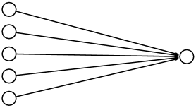
Figure 13.1: Graphical illustration of a linear model as a network: feature values are input nodes, arrows are weights, and the score is an output node.

Most prominently, we use linear models to combine different components of a machine translation system, such as the language model, the phrase translation model, the reordering model, and properties such as the length of the sentence, or the accumulated jump distance between phrase translations. Training methods assign a weight value $\lambda_{i}$ to each such feature $h_{i}(x)$, related to their importance in contributing to scoring better translations higher. In statistical machine translation, this is called tuning.

However, linear models do not allow us to define more complex relationships between the features. Let us say that we find that for short sentences the language model is less important than the translation model, or that average phrase translation probabilities higher than 0.1 are similarly reasonable but any value below that is really terrible. The first hypothetical example implies dependence between features and the second example implies non-linear relationship between the feature value and its impact on the final score. Linear models cannot handle these cases.

A commonly cited counter-example to the use of linear models is XOR, i.e., the boolean operator $\oplus$ with the truth table $0\oplus 0=0$, $1\oplus 0=1$, $0\oplus 1=1$, and $1\oplus 1=0$. For a linear model with two features (representing the inputs), it is not possible to come up with weights that give the correct output in all cases. Linear models assume that all instances, represented as points in the feature space, are linearly separable. This is not the case with XOR, and may not be the case for type of features we use in machine translation.

Multiple Layers

Neural networks modify linear models in two important ways. The first is the use of multiple layers. Instead of computing the output value directly from the input values, a hidden layer is introduced. It is called hidden, because we can observe inputs and outputs in training instances, but not the mechanism that connects them — this use of the concept hidden is similar to its meaning in hidden Markov models.

See Figure 13.2 for on illustration. The network is processed in two steps. First, a linear combination of weighted input node is computed to produce each hidden node value. Then a linear combination of weighted hidden nodes is computed to produce each output node value.

At this point, let us introduce mathematical notations from the neural network literature. A neural network with a hidden layer consists of

• a vector of input nodes with values $\vec{x}=(x_{1},x_{2},x_{3},...x_{n})^{T}$

• a vector of hidden nodes with values $\vec{h}=(h_{1},h_{2},h_{3},...h_{m})^{T}$

• a vector of output nodes with values $\vec{y}=(y_{1},y_{2},y_{3},...y_{l})^{T}$

• a matrix of weights connecting input nodes with hidden nodes $W=\{w_{ij}\}$

• a matrix of weights connecting hidden nodes with output nodes $U=\{u_{ij}\}$

The computations in a neural network with a hidden layer, as sketched out so far, are

$$h_{j}=\sum_{i}x_{i}w_{ji}$$ (13.2)

$$y_{k}=\sum_{j}h_{j}u_{kj}$$ (13.3)

Note that we snuck in the possibility of multiple output nodes $y_{k}$, although our figures so far only showed one.

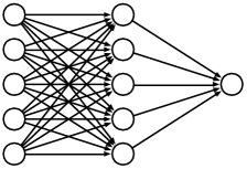
Figure 13.2: A neural network with a hidden layer.

Non-Linearity

If we carefully think about the addition of a hidden layer, we realize that we have not gained anything so far to model input/output relationships. We can easily do away with the hidden layer by multiplying out the weights

$$\begin{split}y_{k}&=\sum_{j}h_{j}u_{kj}\\ &=\sum_{j}\sum_{i}x_{i}w_{ji}u_{kj}\\ &=\sum_{i}x_{i}\left(\sum_{j}u_{kj}w_{ji}\right)\end{split}$$ (13.4)

Hence, a salient element of neural networks is the use of a non-linear activation function. After computing the linear combination of weighted feature values $s_{j}=\sum_{i}x_{i}w_{ji}$, we obtain the value of a node only after applying such a function $h_{j}=f(s_{j})$.

Hyperbolic tangent	Logistic function	Rectified linear unit
tanh($x)=\frac{\text{sinh}(x)}{\text{cosh}(x)}=\frac{e^{x}-e^{-x}}{e^{x}+e^{-x}}$	sigmoid$(x)=\frac{1}{1+e^{-x}}$	relu($x$) = max(0,$x$)
output ranges	output ranges	output ranges
from –1 to +1	from 0 to +1	from 0 to $\infty$

Figure 13.3: Typical activation functions in neural networks.

Popular choices are the hyperbolic tangent tanh(x) and the logistic function sigmoid(x). See Figure 13.3 for more details on these functions. A good way to think about these activation functions is that they segment the range of values for the linear combination $s_{j}$ into

• a segment where the node is turned off (values close to 0 for tanh, or –1 for sigmoid)

• a transition segment where the node is partly turned on

• a segment where the node is turned on (values close to 1)

A different popular choice is the activation function for the rectified linear unit (ReLU). It does not allow for negative values and floors them at 0, but does not alter the value of positive values. It is simpler and faster to compute than tanh($x$) or sigmoid($x$).

You could view each hidden node as a feature detector. For a certain configurations of input node values, it is turned on, for others it is turned off. Advocates of neural networks claim that the use of hidden nodes obviates (or at least drastically reduces) the need for feature engineering: Instead of manually detecting useful patterns in input values, training of the hidden nodes discovers them automatically.

We do not have to stop at a single hidden layer. The currently fashionable name deep learning for neural networks stems from the fact that often better performance can be achieved by deeply stacking together layers and layers of hidden nodes.

Inference

Let us walk through neural network i̱nference (i.e., how output values are computed from input values) with a concrete example. Consider the neural network in Figure 13.4. This network has one additional innovation that we have not presented so far: bias units. These are nodes that always have the value 1. Such bias units give the network something to work with in the case that all input values are 0. Otherwise, the weighted sum $s_{j}$ would be 0 no matter the weights.

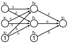
Figure 13.4: A simple neural network with bias nodes in input and hidden layers.

Let us use this neural network to process some input, say the value 1 for the first input node $x_{0}$ and 0 for the second input node $x_{1}$. The value of the bias input node (labelled $x_{2}$) is fixed to 1. To compute the value of the first hidden node $h_{0}$, we have to carry out the following calculation.

$$\begin{split}h_{0}&=\text{sigmoid}\left(\sum_{i}x_{i}w_{1i}\right)\\ &=\text{sigmoid}\left(1\times 3+0\times 4+1\times-2\right)\\ &=\text{sigmoid}\left(1\right)\\ &=0.73\end{split}$$ (13.5)

The calculations for the other nodes are summarized in Table 13.1. The output value in node $y_{0}$ for the input (0,1) is 0.743. If we expect binary output, we would understand this result as the value 1, since it is over the threshold of 0.5 in the range of possible output values [0;1].

Layer	Node	Summation	Activation
hidden	$h_{0}$	$1\times 3+0\times 4+1\times-2=1$	0.731
hidden	$h_{1}$	$1\times 2+0\times 3+1\times-4=-2$	0.119
output	$y_{0}$	$0.731\times 5+0.119\times-5+1\times-2=1.060$	0.743

Table 13.1: Calculations for input (1,0) to the network in Figure 13.4.

Here, the output for all possible binary inputs:

Input $x_{0}$	Input $x_{1}$	Hidden $h_{0}$	Hidden $h_{1}$	Output $y_{0}$
0	0	0.119	0.018	0.183 $\rightarrow$ 0
0	1	0.881	0.269	0.743 $\rightarrow$ 1
1	0	0.731	0.119	0.743 $\rightarrow$ 1
1	1	0.993	0.731	0.334 $\rightarrow$ 0

Our neural network computes xor. How does it do that? If we look at the hidden nodes $h_{0}$ and $h_{1}$, we notice that $h_{0}$ acts like the Boolean or: Its value is high if at least of the two input values is 1 ($h_{0}$ = 0.881, 0.731, 0.993, for the three configurations), it otherwise has a low value (0.119). The other hidden node $h_{1}$ acts like the Boolean and — it only has a high value (0.731) if both inputs are 1. xor is effectively implemented as the subtraction of the and from the or hidden node.

Note that the non-linearity is key here. Since the value for the or node $h_{0}$ is not that much higher for the input of (1,1) opposed to a single 1 in the input (0.993 vs. 0.881 and 0.731), the distinct high value for the and node $h_{1}$ in this case (0.731) manages to push the final output $y_{0}$ below the threshold. This would not be possible if the values of the inputs would be simply summed up as in linear models.

As mentioned before, recently the use of the name deep learning for neural networks has become fashionable. It emphasizes that often higher performance can be achieved by using networks with multiple hidden layers. Our xor example hints at where this power comes from. With a single input-output layer network it is possible to mimic basic Boolean operations such as and and or since they can be modeled with linear classifiers. xor can be expressed as $x\;\text{\sc and}\;y-x\;\text{\sc or}\;y$, and our neural network example implements the Boolean operations and and or in the first layer, and the subtraction in the second layer. For functions that require more intricate computations, more operations may be chained together, and hence a neural network architecture with more hidden layers may be needed. It may be possible (with sufficient training data) to build neural networks for any computer program, if the number of hidden layers matches the depth of the computation. There is a line of research under the banner neural Turing machines that explores what kind of architectures are needed to implement basic algorithms (Gemici et al., 2017). For instance, a neural network with two hidden layers is sufficient to implement an algorithm that sorts $n$-bit numbers.

Back-Propagation Training

Training neural networks requires the optimization of weight values so that the network predicts the correct output for a set of training examples. We repeatedly feed the input from the training examples into the network, compare the computed output of the network with the correct output from the training example, and update the weights. Typically, several passes over the training data are carried out. Each pass over the data is called an epoch.

The most common training method for neural networks is called back-propagation, since it first updates the weights to the output layer, and propagates back error information to earlier layers. Whenever a training example is processed, then for each node in the network, an error term is computed which is the basis for updating the values for incoming weights.

The formulas used to compute updated values for weights follows principles of gradient descent training. The error for a specific node is understood as a function of the incoming weights. To reduce the error given this function, we compute the gradient of the error function with respect to each of the weights, and move against the gradient to reduce the error.

Why is moving alongside the gradient a good idea? Consider that we optimize multiple dimensions at the same time. If you are looking for the lowest point in an area (maybe you are looking for water in a desert), and the ground falls off steep to the west of you, and also slightly south of you, then you would go in a direction that is mainly west — and only slightly south. In other words, you go alongside the gradient. See Figure 13.5 for an illustration.

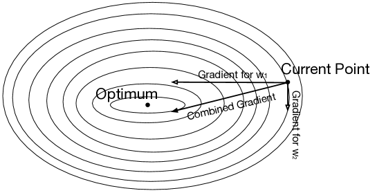
Figure 13.5: Gradient descent training: We compute the gradient with regard to every dimension. In this case the gradient with respect to weight $w_{2}$ smaller than the gradient with respect to the weight $w_{1}$, so we move more to the left than down (note: arrows point in negative gradient direction, pointing to the minimum).

In the following two sections, we will derive the formulae for updating weights for our example network. If you are less interested in the why and more in the how, you can skip these sections and continue reading when we summarize the update formulae 13.2.5.

Weights to the output nodes

Let us first review and extend our notation. At an output node $y_{i}$, we first compute a linear combination of weight and hidden node values.

$$s_{i}=\sum_{j}w_{i\leftarrow j}h_{j}$$ (13.6)

This sum $s_{i}$ is passed through an activation function such as sigmoid to compute the output value $y$.

$$y_{i}=\text{sigmoid}(s_{i})$$ (13.7)

We compare the computed output values $y_{i}$ against the target output values $t_{i}$ from the training example. There are various ways to compute an error value $E$ from these values. Let us use the L2 norm.

$$E=\sum_{i}\frac{1}{2}(t_{i}-y_{i})^{2}$$ (13.8)

As we stated above, our goal is to compute the gradient of the error $E$ with respect to the weights $w_{k}$ to find out in which direction (and how strongly) we should move the weight value. We do this for each weight $w_{k}$ separately. We first break up the computation of the gradient into three steps, essentially unfolding the Equations 13.6 to 13.8.

$$\frac{dE}{dw_{i\leftarrow j}}=\frac{dE}{dy_{i}}\frac{dy_{i}}{ds_{i}}\frac{ds_{i}}{dw_{i\leftarrow j}}$$ (13.9)

Let us now work through each of these three steps.

• Since we defined the error $E$ in terms of the output values $y_{i}$, we can compute the first component as follows.

  $$\frac{dE}{dy_{i}}=\frac{d}{dy_{i}}\;\frac{1}{2}(t_{i}-y_{i})^{2}=-(t_{i}-y_{i})$$ (13.10)

• The derivative of the output value $y_{i}$ with respect to $s_{i}$ (the linear combination of weight and hidden node values) depends on the activation function. In the case of sigmoid, we have:

  $$\frac{dy_{i}}{ds_{i}}=\frac{d\;\text{sigmoid}(s_{i})}{ds_{i}}=\text{sigmoid}(s_{i})(1-\text{sigmoid}(s_{i}))=y_{i}(1-y_{i})$$ (13.11)

  To keep our treatment below as general as possible and not commit to the sigmoid as an activation function, we will use the shorthand $y^{\prime}_{i}$ for $\frac{dy_{i}}{ds_{i}}$ below. Note that for any given training example and any given differentiable activation function, this value can always be computed.

• Finally, we compute the derivative of $s_{i}$ with respect to the weight $w_{i\leftarrow j}$, which turns out to be quite simply the value to the hidden node $h_{j}$.

  $$\frac{ds}{dw_{i\leftarrow j}}=\frac{d}{dw_{i\leftarrow j}}\sum_{j}w_{i\leftarrow j}h_{j}=h_{j}$$ (13.12)

Where are we? In Equations 13.10 to 13.12, we computed the three steps needed to compute the gradient for the error function given the unfolded laid out in Equation 13.9. Putting it all together, we have

$$\begin{split}\frac{dE}{dw_{i\leftarrow j}}&=\frac{dE}{dy_{i}}\frac{dy_{i}}{ds_{i}}\frac{ds}{dw_{i\leftarrow j}}\\ &=-(t_{i}-y_{i})\;\;\;y^{\prime}_{i}\;\;\;h_{j}\end{split}$$ (13.13)

Factoring in a learning rate $\mu$ gives us the following update formula for weight $w_{i\leftarrow j}$. Note that we also remove the minus sign, since we move against the gradient towards the minimum.

$$\Delta w_{i\leftarrow j}=\mu(t_{i}-y_{i})\;y_{i}^{\prime}\;h_{j}$$

It is useful to introduce the concept of an error term $\delta_{i}$. Note that this term is associated with a node, while the weight updates concern weights. The error term has to be computed only once for the node, and it can be then used for each of the incoming weights.

$$\delta_{i}=(t_{i}-y_{i})\;y^{\prime}_{i}$$ (13.14)

This reduces the update formula to:

$$\Delta w_{i\leftarrow j}=\mu\;\delta_{i}\;h_{j}$$ (13.15)

Weights to the hidden nodes

The computation of the gradient and hence the update formula for hidden nodes is quite analogous. As before, we first define the linear combination $z_{j}$ (previously $s_{i}$) of input values $x_{k}$ (previously hidden values $h_{j}$) weighted by weights $u_{j\leftarrow k}$ (previously weights $w_{i\leftarrow j}$).

$$z_{j}=\sum_{k}u_{j\leftarrow k}x_{k}$$ (13.16)

This leads to the computation of the value of the hidden node $h_{j}$.

$$h_{j}=\text{sigmoid}(z_{j})$$ (13.17)

Following the principles of gradient descent, we need to compute the derivative of the error $E$ with respect to the weights $u_{j\leftarrow k}$. We decompose this derivative as before.

$$\frac{dE}{du_{j\leftarrow k}}=\frac{dE}{dh_{j}}\frac{dh_{j}}{dz_{j}}\frac{dz_{j}}{du_{j\leftarrow k}}$$ (13.18)

However, the computation of $\frac{dE}{dh_{j}}$ is more complex than in the case of output nodes, since the error is defined in terms of output values $y_{i}$, not values for hidden nodes $h_{j}$. The idea behind back-propagation is to track how the error caused by the hidden node contributed to the error in the next layer. Applying the chain rule gives us:

$$\frac{dE}{dh_{j}}=\sum_{i}\frac{dE}{dy_{i}}\frac{dy_{i}}{ds_{i}}\frac{ds_{i}}{dh_{j}}$$ (13.19)

We already encountered the first two terms $\frac{dE}{dy_{i}}$ (Equation 13.10) and $\frac{dy_{i}}{ds_{i}}$ (Equation 13.11) previously. To recap:

$$\begin{split}\frac{dE}{dy_{i}}\;\frac{dy_{i}}{ds_{i}}&=\frac{d}{dy_{i}}\;\sum_{i^{\prime}}\frac{1}{2}(t_{i}-y_{i^{\prime}})^{2}\;\;\;y^{\prime}_{i}\\ &=\frac{d}{dy_{i}}\frac{1}{2}(t_{i}-y_{i})^{2}\;\;\;y^{\prime}_{i}\\ &=-(t_{i}-y_{i})\;\;\;y^{\prime}_{i}\\ &=\delta_{i}\end{split}$$ (13.20)

The third term in Equation 13.19 is computed straightforward.

$$\frac{ds_{i}}{dh_{j}}=\frac{d}{dh_{j}}\sum_{i}w_{i\leftarrow j}h_{j}=w_{i\leftarrow j}$$ (13.21)

Putting Equation 13.20 and Equation 13.21 together, Equation 13.19 can be solved as:

$$\frac{dE}{dh_{j}}=\sum_{i}\delta_{i}w_{i\leftarrow j}$$ (13.22)

This gives rise to a quite intuitive interpretation. The error that matters at the hidden node $h_{j}$ depends on the error terms $\delta_{i}$ in the subsequent nodes $y_{i}$, weighted by $w_{i\leftarrow j}$, i.e., the impact the hidden node $h_{j}$ has on the output node $y_{i}$.

Let us tie up the remaining loose ends. The missing pieces from Equation 13.18 are the second term

$$\frac{dh_{j}}{dz_{j}}=\frac{d\;\text{sigmoid}(z_{j})}{dz_{j}}=\text{sigmoid}(z_{j})(1-\text{sigmoid}(z_{j}))=h_{j}(1-h_{j})=h^{\prime}_{j}$$ (13.23)

and third term

$$\frac{dz_{j}}{du_{j\leftarrow k}}=\frac{d}{du_{j\leftarrow k}}\sum_{k}u_{j\leftarrow k}x_{k}=x_{k}$$ (13.24)

Putting Equation 13.22, Equation 13.23, and Equation 13.24 together gives us the gradient

$$\begin{split}\frac{dE}{du_{j\leftarrow k}}&=\frac{dE}{dh_{j}}\frac{dh_{j}}{dz_{j}}\frac{dz_{j}}{du_{j\leftarrow k}}\\ &=\sum_{i}\left(\delta_{i}w_{i\leftarrow j}\right)\;\;h^{\prime}_{j}\;\;x_{k}\end{split}$$ (13.25)

If we define an error term $\delta_{j}$ for hidden nodes analogous to output nodes

$$\delta_{j}=\sum_{i}\left(\delta_{i}w_{i\leftarrow j}\right)\;\;h^{\prime}_{j}$$ (13.26)

then we have an analogous update formula

$$\Delta u_{j\leftarrow k}=\mu\;\delta_{j}\;x_{k}$$ (13.27)

Summary

We train neural networks by processing training examples, one at a time, and update weights each time. What drives weight updates is the gradient towards a smaller error. Weight updates are computed based on error terms $\delta_{i}$ associated with each non-input node in the network.

For output nodes, the error term $\delta_{i}$ is computed from the actual output $y_{i}$ of the node for our current network, and the target output $t_{i}$ for the node.

$$\delta_{i}=(t_{i}-y_{i})\;y^{\prime}_{i}$$ (13.28)

For hidden nodes, the error term $\delta_{j}$ is computed via back-propagating the error term $\delta_{i}$ from subsequent nodes connected by weights $w_{i\leftarrow j}$.

$$\delta_{j}=\sum_{i}\left(\delta_{i}w_{i\leftarrow j}\right)\;h^{\prime}_{j}$$ (13.29)

Computing $y^{\prime}_{i}$ and $h^{\prime}_{j}$ requires the derivative of the activation function, to which the weighted sum of incoming values is passed.

Given the error terms, weights $w_{i\leftarrow j}$ (or $u_{j\leftarrow k}$) from each proceeding node $h_{j}$ (or $x_{k}$) are updated, tempered by a learning rate $\mu$.

$$\begin{split}\Delta w_{i\leftarrow j}&=\mu\;\delta_{i}\;h_{j}\\ \Delta u_{j\leftarrow k}&=\mu\;\delta_{j}\;x_{k}\end{split}$$ (13.30)

Once weights are updated, the next training example is processed. There are typically several passes over the training set, called epochs.

Example

Given the neural network in Figure 13.4, let us see how the training example (1,0) $\rightarrow$ 1 is processed.

Let us start with the calculation of the error term $\delta$ for the output node $y_{0}$. During inference (recall Table 13.1), we computed the linear combination of weighted hidden node values $s_{0}=1.060$ and the node value $y_{0}=0.743$. The target value is $t_{0}=1$.

$$\delta=(t_{0}-y_{0})\;y^{\prime}_{0}=(1-0.743)\times\text{sigmoid}^{\prime}(1.060)=0.257\times 0.191=0.049$$ (13.31)

With this number, we can compute weight updates, such as for weight $w_{0\leftarrow 0}$.

$$\Delta w_{0\leftarrow 0}=\mu\;\delta_{0}\;h_{0}=\mu\times 0.049\times 0.731=\mu\times 0.036$$ (13.32)

Since the hidden node $h_{0}$ leads only to one output node $y_{0}$, the calculation of its error term $\delta_{0}$ is not more computationally complex.

$$\delta_{j}=\sum_{i}\left(\delta_{i}u_{i\leftarrow 0}\right)\;h^{\prime}_{0}=\left(\delta\times w_{0\leftarrow 0}\right)\times\text{sigmoid}^{\prime}(z_{0})=0.049\times 5\times 0.197=0.049$$ (13.33)

Table 13.2 summarizes the updates for all weights.

Node	Error term	Weight updates
	$\delta=(t_{0}-y_{0})\;\text{sigmoid}(s_{0})$	$\Delta w_{0\leftarrow j}=\mu\;\delta\;h_{j}$
$y_{0}$	$\delta=(1-0.743)\times 0.191=0.049$	$\Delta w_{0\leftarrow 0}=\mu\times 0.049\times 0.731=0.036$
		$\Delta w_{0\leftarrow 1}=\mu\times 0.049\times 0.119=0.006$
		$\Delta w_{0\leftarrow 2}=\mu\times 0.049\times 1=0.049$
	$\delta_{j}=\delta\;w_{i\leftarrow j}\;\text{sigmoid}(z_{j})$	$\Delta u_{j\leftarrow i}=\mu\;\delta_{j}\;x_{i}$
$h_{0}$	$\delta_{0}=0.049\times 5\times 0.197=0.048$	$\Delta u_{0\leftarrow 0}=\mu\times 0.048\times 1=0.048$
		$\Delta u_{0\leftarrow 1}=\mu\times 0.048\times 0=0$
		$\Delta u_{0\leftarrow 2}=\mu\times 0.048\times 1=0.048$
$h_{1}$	$\delta_{1}=0.049\times-5\times 0.105=-0.026$	$\Delta u_{1\leftarrow 0}=\mu\times-0.026\times 1=-0.026$
		$\Delta u_{1\leftarrow 1}=\mu\times-0.026\times 0=0$
		$\Delta u_{1\leftarrow 2}=\mu\times-0.026\times 1=-0.026$

Table 13.2: Weight updates (with unspecified learning rate $\mu$) for the neural network in Figure 13.4 (repeated above the table) when the training example (1,0) $\rightarrow$ 1 is presented.

Refinements

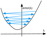
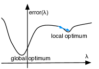
Too high learning rate	Bad initialization	Local optimum

Figure 13.6: Problems with gradient descent training that motivate some of the refinements detailed in Section 13.2.6: (a) a too high learning rate may lead to too drastic parameter updates, overshooting the optimum, (b) bad initialization may require many updates to escape a plateau, and (c) the existence of local optima which trap training.

We conclude our introduction to neural networks with some basic refinements and considerations. To motivate some of the refinements, consider Figure 13.6. While gradient descent training is a fine idea, it may run into practical problems.

• Setting the learning rate too high leads to updates that overshoot the optimum. Conversely, a too low learning rate leads to slow convergence.

• Bad initialization of weights may lead to long paths of many update steps to reach the optimum. This is especially a problem with activation functions like sigmoid which only have a short interval of significant change.

• The existence of local optima lead the search to get trapped and miss the global optimum.

Validation Set

Neural network training proceeds for several epochs, i.e., full iterations over the training data. When to stop? When we track training progress, we see that the error on the training set continuously decreases. However, at some point over-fitting sets in, where the training data is memorized and not sufficiently generalized.

We can check this with an additional set of examples, called the validation set, that is not used during training. See Figure 13.7 for an illustration. When we measure the error on the validation set at each point of training, we see that at some point this error increases. Hence, we stop training, when the minimum on the validation set is reached.

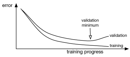
Figure 13.7: Training progress over time. The error on the training set continuously decreases. However, on a validation set (not used for training), at some point the error increases. Training is stopped at the validation minimum before such over-fitting sets in.

Weight Initialization

Before training starts, weights are initialized to random values. The values are choses from a uniform distribution. We prefer initial weights that lead to node values that are in the transition area for the activation function, and not in the low or high shallow slope where it would take a long time to push towards a change. For instance, for the sigmoid activation function, feeding values in the range of, say, $[-1;1]$ to the activation function leads to activation values in the range of [0.269;0.731].

For the sigmoid activation function, commonly used formula for weights to the final layer of a network are

$$\big{[}-\frac{1}{\sqrt{n}},\frac{1}{\sqrt{n}}\big{]}$$ (13.34)

where $n$ is the size of the previous layer. For hidden layers, we chose weights from the range

$$\big{[}-\frac{\sqrt{6}}{\sqrt{n_{j}+n_{j+1}}},\frac{\sqrt{6}}{\sqrt{n_{j}+n_{j+1}}}\big{]}$$ (13.35)

where $n_{j}$ is the size of the previous layer, $n_{j}$ size of next layer.

Momentum Term

Consider the case where a weight value is far from its optimum. Even if most training examples push the weight value in the same direction, it may still take a while for each of these small updates to accumulate until the weight reaches its optimum. A common trick is to use a momentum term to speed up training. This momentum term $m_{t}$ gets updated at each time step $t$ (i.e., for each training example). We combine the previous value of the momentum term $m_{t-1}$ with the current raw weight update value $\Delta w_{t}$ and use the resulting momentum term value to update the weights.

For instance, with a decay rate of 0.9, the update formula changes to

$$\begin{split}m_{t}&=0.9m_{t-1}+\Delta w_{t}\\ w_{t}&=w_{t-1}-\mu\;m_{t}\end{split}$$ (13.36)

Adapting Learning Rate per Parameter

A common training strategy is to reduce the learning rate $\mu$ over time. At the beginning the parameters are far away from optimal values and have to change a lot, but in later training stages we are concerned with fine tuning, and a large learning rate may cause a parameter to bounce around an optimum.

But different parameters may be at different stages on the path to their optimal values, so a different learning rate for each parameter may be helpful. One such method, called Adagrad, records the gradients that were computed for each parameter and accumulates their square values over time, and uses this sum to adjust the learning rate.

The Adagrad update formula is based on the sum of gradients of the error $E$ with respect to the weight $w$ at all time steps $t$, i.e., $g_{t}=\frac{dE_{t}}{dw}$. We divide the learning rate $\mu$ for this weight this accumulated sum.

$$\Delta w_{t}=\frac{\mu}{\sqrt{\sum_{\tau=1}^{t}g_{\tau}^{2}}}\;g_{t}$$ (13.37)

Intutively, big changes in the parameter value (corresponding to big gradients $g_{t}$), lead to a reduction of the learning rate of the weight parameter.

Combining the idea of momentum term and adjusting parameter update by their accumulated change is the inspiration of Adam, another method to transform the raw gradient into a parameter update.

First, there is the idea of momentum, which is computed as in Equation 13.36 above.

$$m_{t}=\beta_{1}m_{t-1}+(1-\beta_{1})g_{t}$$ (13.38)

Then, there is the idea of the squares of gradients (as in Adagrad) for adjusting the learning rate. Since raw accumulation does run the risk of becoming too large and hence permanently depressing the learning rate, Adam uses exponential decay, just like for the momentum term.

$$v_{t}=\beta_{2}v_{t-1}+(1-\beta_{2})g_{t}^{2}$$ (13.39)

The hyper parameters $\beta_{1}$ and $\beta_{2}$ are set typically close to 1, but this also means that early in training the values for $m_{t}$ and $v_{t}$ are close to their initialization values of 0. To adjust for that, they are corrected for this bias.

$$\hat{m}_{t}=\frac{m_{t}}{1-\beta^{t}_{1}},\hskip 28.45274pt\hat{v}_{t}=\frac{v_{t}}{1-\beta^{t}_{2}}$$ (13.40)

With increasing training time steps $t$, this correction goes away: $\text{lim}_{t\rightarrow\infty}\frac{1}{1-\beta^{t}}\rightarrow 1$.

Having these pieces in hand (learning rate $\mu$, momentum $\hat{m}_{t}$, accumulated change $\hat{v}_{t}$), weight update per Adam is computed as

$$\Delta w_{t}=\frac{\mu}{\sqrt{\hat{v}_{t}}+\epsilon}\hat{m}_{t}$$ (13.41)

Common values for the hyper parameters are $\beta_{1}=0.9$, $\beta_{2}=0.999$ and $\epsilon=10^{-8}$.

There are various other adaptation schemes. This is an active area of research. For instance, the second order gradient gives some useful information about the rate of change. However, it is often expensive to compute, so other shortcuts are taken.

Dropout

The parameter space in which back-propagation learning and its variants are operating is littered with local optima. The hill-climbing algorithm may just climb a mole hill and be stuck there, instead of moving towards a climb of the highest mountain. Various methods have been proposed to get training out of these local optima. One currently popular method in neural machine translation is called drop-out.

It sounds a bit simplistic and wacky. During training, some of the nodes of the neural network are ignored. Their values are set to 0, and their associated parameters are not updated. These dropped-out nodes are chosen at random, and may account for as much as 10%, 20% or even more of all the nodes. Training resumes for some number of iterations without the nodes, and then a different set of drop-out nodes are selected.

The dropped-out nodes played some useful role in the model trained up to the point where they are ignored. After that, other nodes have to pick up the slack. The end result is a more robust model where several nodes share similar roles.

Layer Normalization

Layer normalization addresses a problem that arises especially in the deep neural networks that we are using in neural machine translation, where computing proceeds through a large sequence of layers. For some training examples, average values at one layer may become very large, which feed into the following layer, also producing large output values, and so on. This is especially a problem with activation functions that do not limit the output to a narrow interval, such as rectified linear units. For other training examples the average values at the same layers may be very small. This causes a problem for training. Recall from Equation 13.30, that gradient updates are strongly effected by node values. Too large node values lead to exploding gradients and too small node values lead to diminishing gradients.

To remedy this, the idea is to normalize the values on a per-layer basis. This is done by adding additional computational steps to the neural network. Recall that a feed-forward layer consists of the the matrix multiplication of the weight matrix $W$ with the node values from the previous layer $\vec{h^{l-1}}$, resulting in a weighted sum $\vec{s^{l}}$, followed by an activation function such as sigmoid.

$$\vec{s^{l}} =W\;\vec{h^{l-1}}$$ (13.42)

$$\vec{h^{l}} =\text{sigmoid}(\vec{h^{l}})$$

We can compute the mean and variance of the values in the weighted sum vector $\vec{s^{l}}$ by

$$\mu^{l} =\frac{1}{H}\sum_{i-1}^{H}s_{i}^{l}$$ (13.43)

$$\sigma^{l} =\sqrt{\frac{1}{H}\sum_{i-1}^{H}(s_{i}^{l}-\mu^{l})^{2}}$$

Using these values, we normalize the vector $\vec{s^{l}}$ using two additional bias vectors $\vec{g}$ and $\vec{b}$

$$\vec{\hat{s^{l}}}=\frac{\vec{g}}{\sigma^{l}}\cdot(\vec{s^{l}}-\mu^{l})+\vec{b}$$ (13.44)

where $\cdot$ is element-wise multiplication and the difference subtracts the scalar average from each vector element.

The formula first normalizes the values in $\vec{s^{l}}$ by shifting them against their average value, hence ensuring that their average afterwards is 0. The resulting vector is then divided by the variance $\sigma^{l}$. The additional bias vectors give some flexibility, they may be shared across multiple layers of the same type, such as multiple time steps in a recurrent neural network (we will introduce these in Section 13.4.4).

Mini Batches

Each training example yields a set of weight updates $\Delta w_{i}$. We may first process all the training examples and only afterwards apply all the updates. But neural networks have the advantage that they can immediately learn from each training example. A training method that updates the model with each training example is called online learning. The online learning variant of gradient descent training is called stochastic gradient descent.

Online learning generally takes fewer passes over the training set (called epochs) for convergence. However, since training constantly changes the weights, it is hard to parallelize. So, instead, we may want to process the training data in batches, accumulate the weight updates, and then apply them collectively. These smaller sets of training examples are called mini batches to distinguish this approach from batch training where the entire training set is considered one batch.

There are other variations to organize the processing of the training set, typically motivated by restrictions of parallel processing. If we process the training data in mini batches, then we can parallelize the computation of weight update values $\Delta w$, but have to synchronize their summation and application to the weights. If we want to distribute training over a number of machines, it is computationally more convenient to break up the training data in equally sized parts, perform online learning for each of the parts (optionally using smaller mini batches), and then average the weights. Surprisingly, breaking up training this way, often leads to better results than straightforward linear processing.

Finally, a scheme called Hogwild runs several training threads that immediately update weights, even though other threads still use the weight values to compute gradients. While this is clearly violates the safe guards typically taken in parallel programming, it does not hurt in practical experience.

Vector and Matrix Operations

We can express the calculations needed for handling neural networks as vector and matrix operations.

• Forward computation: $\vec{s}=W\;\vec{h}$

• Activation function: $\vec{y}=\text{sigmoid}(\vec{h})$

• Error term: $\vec{\delta}=(\vec{t}-\vec{y})\;\text{sigmoid'}(\vec{s})$

• Propagation of error term: $\vec{\delta}_{i}=W\;\vec{\delta}_{i+1}\cdot\text{sigmoid'}(\vec{s})$

• Weight updates: $\Delta W=\mu\;\vec{\delta}\;\vec{h}^{T}$

Executing these operations is computationally expensive. If our layers have, say, 200 nodes, then the matrix operation $W\vec{h}$ requires $200\times 200=40,000$ multiplications. Such matrix operations are also common in another highly used area of computer science: graphics processing. When rendering images on the screen, the geometric properties of 3-dimensional objects have to be processed to generate the color values of the 2-dimensional image on the screen. Since there is high demand for fast graphics processing, for instance for the use in realistic looking computer games, specialized hardware has become commonplace: graphics processing units (GPUs).

These processors have a massive number of cores (for example, the NVIDIA GTX 1080ti GPU provides 3584 thread processors) but a rather lightweight instruction set. GPUs provide instructions that are applied to many data points at once, which is exactly what is needed out the vector space computations listed above. Programming for GPUs is supported by various libraries, such as CUDA for C++, and has become an essential part of developing large scale neural network applications.

The general term for scalars, vectors, and matrices is tensors. A tensor may also have more dimensions: a sequence of matrices can be packed into a 3-dimensional tensor. Such large objects are actually frequently used in today’s neural network toolkits.

Further Readings

A good introduction to modern neural network research is the textbook ”Deep Learning” (Goodfellow et al., 2016). There is also book on neural network methods applied to the natural language processing in general (Goldberg, 2017).

A number of key techniques that have been recently developed have entered the standard repertoire of neural machine translation research. Training is made more robust by methods such as drop-out (Srivastava et al., 2014), where during training intervals a number of nodes are randomly masked. To avoid exploding or vanishing gradients during back-propagation over several layers, gradients are typically clipped (Pascanu et al., 2013). Layer normalization (Lei Ba et al., 2016) has similar motivations, by ensuring that node values are within reasonable bounds.

An active topic of research are optimization methods that adjust the learning rate of gradient descent training. Popular methods are Adagrad (Duchi et al., 2011), Adadelta (Zeiler, 2012), and currently Adam (Kingma and Ba, 2015).

Computation Graphs

For our example neural network from Section 13.2.5, we painstakingly worked out derivates for gradient computations needed by gradient descent training. After all this hard work, it may come as surprise that you will likely never have to do this again. It can be done automatically, even for arbitrarily complex neural network architectures. There are a number of toolkits that allow you to define the network and it will take care of the rest. In this section, we will take a close look at how this works.

Neural Networks as Computation Graphs

First, we will take a different look at the networks we are building. We previously represented neural networks as graphs consisting of nodes and their connections (recall Figure 13.4), or by mathematical equations such as

$$\begin{split}h=\text{sigmoid}(W_{1}x+b_{1})\\ y=\text{sigmoid}(W_{2}h+b_{2})\end{split}$$ (13.45)

The equations above describe the feed-forward neural network that we use as our running example. We now represent this math in form of a computation graph. See Figure 13.8 for an illustration of the computation graph for our network. The graph contains as nodes the parameters of the models (the weight matrices $W_{1}$, $W_{2}$ and bias vectors $b_{1}$, $b_{2}$), the input $x$ and the mathematical operations that are carried out between them (product, sum, and sigmoid). Next to each parameter, we show their values.

Figure 13.8: Two layer feed-forward neural network as a computation graph, consisting of the input value $x$, weight parameters $W_{1}$, $W_{2}$, $b_{1}$, $b_{2}$, and computation nodes (product, sum, sigmoid). To the right of each parameter node, its value is shown. To the left of input and computation nodes, we show how the input $(1,0)^{T}$ is processed by the graph.

Neural networks, viewed as computation graphs, are any arbitrary connected operations between an input and any number of parameters. Some of these operations may have little to do with any inspiration from neurons in the brain, so we are stretching the term neural networks quite a bit here. The graph does not have to have a nice tree structure as in our example, but may be any acyclical directed graph, i.e., anything goes as long there is a straightforward processing direction and no cycles. Another way to view such a graph is as a fancy way to visualize a sequence of function calls that take as arguments the input, parameters, previously computed values, or any combination thereof, but have no recursion or loops.

Processing an input with the neural network requires placing the input value into the node $x$ and carrying out the computations. In the figure, we show this with the input vector $(1,0)^{T}$. The resulting numbers should look familiar since they are the same as when previously worked through this example in Section 13.2.4.

Before we move on, let us take stock of what each computation node in the graph has to accomplish. It consists of the following:

• a function that executes its computation operation

• links to input nodes

• when processing an example, the computed value

We will add two more items to each node in the following section.

Gradient Computations

So far, we showed how the computation graph can be used process an input value. Now we will examine how it can be used to vastly simply model training. Model training requires an error function and the computation of gradients to derive update rules for parameters.

The first of these is quite straightforward. To compute the error, we need to add another computation at the end of the computation graph. This computation takes the computed output value $y$ and the given correct output value $t$ from the training data and produces an error value. A typical error function is the L2 norm $\frac{1}{2}(t-y)^{2}$. From the view of training, the result of the execution of the computation graph is an error value.

Calculus Refresher
In calculus, the chain rule is a formula for computing the derivative of the composition of two or more functions. That is, if f and g are functions, then the chain rule expresses the derivative of their composition $f\cdot g$ (the function which maps $x$ to $f(g(x))$) in terms of the derivatives of $f$ and $g$ and the product of functions as follows: $(f\circ g)^{\prime}=(f^{\prime}\circ g)\cdot g^{\prime}.$ This can be written more explicitly in terms of the variable. Let $F=f\cdot g$, or equivalently, $F(x)=f(g(x))$ for all $x$. Then one can also write $F^{\prime}(x)=f^{\prime}(g(x))g^{\prime}(x)$ The chain rule may be written, in Leibniz’s notation, in the following way. If a variable z depends on the variable $y$, which itself depends on the variable $x$, so that $y$ and $z$ are therefore dependent variables, then $z$, via the intermediate variable of $y$, depends on $x$ as well. The chain rule then states, $\frac{dz}{dx}=\frac{dz}{dy}\cdot\frac{dy}{dx}$ The two versions of the chain rule are related, if $z=f(y)$ and $y=g(x)$, then $\frac{dz}{dx}=\frac{dz}{dy}\cdot\frac{dy}{dx}=f^{\prime}(y)g^{\prime}(x)=f^{\prime}(g(x))g^{\prime}(x)$ (adapted from Wikipedia)

Now, for the more difficult part — devising update rules for the parameters. Looking at the computation graph, model updates originate from the error values and propagate back to the model parameter. Hence, we call the computations needed to compute the update values also the backward pass through the graph, opposed to the forward pass that computed output and error.

Consider the chain of operations that connect the weight matrix $W_{2}$ to the error computation.

$$\begin{split}e&=\text{L2}(y,t)\\ y&=\text{sigmoid}(s)\\ s&=\text{sum}(p,b_{2})\\ p&=\text{prod}(h,W_{2})\end{split}$$ (13.46)

where $h$ are the values of the hidden layer nodes, resulting from earlier computations.

To compute the update rule for the parameter matrix $W_{2}$, we view the error as a function of these parameters and take the derivative with respect to them, in our case $\frac{dL2(W_{2})}{dW_{2}}$. Recall that when we computed this derivate we first broke it up into steps using the chain rule. We now do the same here.

$$\frac{d\text{L2}(W_{2})}{dW_{2}}=\frac{d\text{L2}(\text{sigmoid}(\text{sum}(\text{prod}(h,W_{2}),b_{2})),t)}{dW_{2}}=\frac{d\text{L2}(y,t)}{dy}\frac{d\text{sigmoid}(s)}{ds}\frac{d\text{sum}(p,b_{2})}{dp}\frac{d\text{prod}(h,W_{2})}{dW_{2}}$$ (13.47)

Note that for the purpose for computing an update rule for $W_{2}$, we treat all the other variables in this computation (the target value $t$, the bias vector $b_{2}$, the hidden node values $h$) as constants. This breaks up the derivative of the error with respect to the parameters $W_{2}$ into a chain of derivatives along the line of the nodes of the computation graph.

Hence, all we have to do for gradient computations is to come up with derivatives for each node in the computation graph. In our example these are

$$\begin{split}\frac{d\text{L2}(y,t)}{dy}&=\frac{d\frac{1}{2}(t-y)^{2}}{dy}=t-y\\ \frac{d\text{sigmoid}(s)}{ds}&=\text{sigmoid}(s)(1-\text{sigmoid}(s))\\ \frac{d\text{sum}(p,b_{2})}{dp}&=\frac{dp+b_{2}}{dp}=1\\ \frac{d\text{prod}(h,W_{2})}{dW_{2}}&=\frac{dW_{2}h}{dW_{2}}=h\end{split}$$ (13.48)

Figure 13.9: Computation graph with gradients computed in the backward pass for the training example $(0,1)^{T}\rightarrow 1.0$. Gradients are computed with respect to the input of the nodes, so some nodes that have two inputs also have two gradients. See text for details on the computations of the values.

If we want to compute the gradient update for a parameter such as $W_{2}$, we compute values in a backward pass, starting from the error term $y$. See Figure 13.9 for an illustration.

To give more detail on the computation of the gradients in the backward pass, starting at the bottom of the graph:

• For the L2 node, we use the formula

  $$\frac{d\text{L2}(y,t)}{dy}=\frac{d\frac{1}{2}(t-y)^{2}}{dy}=t-y$$ (13.49)

  The given target output value given as training data is $t=1$, while we computed $y=0.743$ in the forward pass. Hence, the gradient for the L2 norm is $1-0.743=0.257$. Note that we are using values computed in the forward pass for these gradient computations.

• For the lower sigmoid node, we use the formula

  $$\frac{d\text{sigmoid}(s)}{ds}=\text{sigmoid}(s)(1-\text{sigmoid}(s))$$ (13.50)

  Recall that the formula for the sigmoid is $\text{sigmoid}(s)=\frac{1}{1+e^{-s}}$. Plugging in the value for $s=1.06$ computed in the forward pass into this formula gives us 0.191. The chain rule requires us to multiply this with the value that we just computed for the L2 node, i.e., 0.257, which gives us $0.191\times 0.257=0.0492$.

• For the lower sum node, we simply copy the previous value, since the derivate is 1:

  $$\frac{d\text{sum}(p,b_{2})}{dp}=\frac{dp+b_{2}}{dp}=1$$ (13.51)

  Note that there are two gradients associated with the sum node. One with respect to the output of the prod node, and one with the $b_{2}$ parameter. In both cases, the derivative is 1, so both values are the same. Hence, the gradient in both cases is 0.0492.

• For the lower prod node, we use the formula

  $$\frac{d\text{prod}(h,W_{2})}{dW_{2}}=\frac{dW_{2}h}{dW_{2}}=h$$ (13.52)

  So far, we dealt with scalar values. Here we encounter vectors for the first time: the value of the hidden nodes $h=(0.731,0.119)^{T}$. The chain rule requires us to multiply this with the previously computed scalar 0.0492:

  $$\Big{(}\begin{bmatrix}0.731\\ 0.119\end{bmatrix}\times 0.0492\Big{)}^{T}=\begin{bmatrix}0.0360&0.00587\end{bmatrix}$$

  As for the sum node, there are two inputs and hence two gradients. The other gradient is with respect to the output of the upper sigmoid node.

  $$\frac{d\text{prod}(h,W_{2})}{dh}=\frac{dW_{2}h}{dh}=W_{2}$$ (13.53)

  Similarly to above, we compute

  $$(W_{2}\times 0.0492)^{T}=\Big{(}\begin{bmatrix}5&-5\end{bmatrix}\times 0.0492\Big{)}^{T}=\begin{bmatrix}0.246\\ -0.246\end{bmatrix}$$

Having all the gradients in place, we can now read of the relevant values for weight updates. These are the gradients associated with trainable parameters. For the $W_{2}$ weight matrix, this is the second gradient of the prod node. So the new value for $W_{2}$ at time step $t+1$ is

$$W_{2}^{t+1}=W_{2}^{t}-\mu\frac{d\text{prod}(x,W_{2}^{t})}{dW_{2}^{t}}=\begin{bmatrix}5&5\end{bmatrix}-\mu\begin{bmatrix}0.0360&0.00587\end{bmatrix}$$ (13.54)

The remaining computations are carried out in very similar fashion, since they form simply another layer of the feed-forward neural network.

Our example did not include one special case: the output of a computation may be used multiple times in subsequent steps of a computation graphs. So, there are multiple output nodes that feed back gradients in the back-propagation pass. In this case, we add up the gradients from these descendent steps to factor in their added impact.

Let us take a second look at what a node in a computation graph comprises:

• a function that computes its value

• links to input nodes (to obtain argument values)

• when processing an example in the forward pass, the computed value

• a function that executes its gradient computation

• links to children nodes (to obtain downstream gradient values)

• when processing an example in the forward pass, the computed gradient

From an object oriented programming view, a node in a computation graph provides a forward and backward function for value and gradient computations. As instantiated in an computation graph, it is connected with specific inputs and outputs, and is also aware of the dimensions of its variables its value and gradient. During forward and backward pass, these variables are filled in.

Deep Learning Frameworks

In the next sections, we will encounter various network architectures. What all of these share, however, are the need for vector and matrix operations, as well as the computation of derivatives to obtain weight update formulas. It would be quite tedious to write almost identical code to deal with each these variants. Hence, a number of frameworks have emerged to support developing neural network methods for any chosen problem. At the time of writing, the most prominent ones are Theano (a Python library that dymanically generates and compiles C++ code and is build on NumPy), Torch (a machine learning library and a script language based on the Lua programming language), pyTorch (the Python variant of Torch), DyNet (a C++ implementation by natural language processing researchers that can be used as a library in C++ or Python), and Tensorflow (a more recent entry to the genre from Google).

These frameworks are less geared towards ready-to-use neural network architectures, but provide efficient implementations of the vector space operations and computation of derivatives, with seamless support of GPUs. Our example from Section 13.2 can be implemented in a few lines of Python code, as we will show in this section, using the example of Theano (other frameworks are quite similar).

You can execute the following commands on the Python command line interface if you first installed Theano (pip install Theano).

> import numpy
> import theano
> import theano.tensor as T

The mapping of the input layer x to the hidden layer h uses a weight matrix W, a bias vector b, and a mapping function which consists of the linear combination T.dot and the sigmoid activation function.

> x = T.dmatrix()
> W = theano.shared(value=numpy.array([[3.0,2.0],[4.0,3.0]]))
> b = theano.shared(value=numpy.array([-2.0,-4.0]))
> h = T.nnet.sigmoid(T.dot(x,W)+b)

Note that we define x as a matrix. This allows us to process several training examples at once (a sequence of vectors). A good way to think about these definitions of x and h is in term of a functional programming language. They symbolically define operations. To actually define a function that can be called, the Theano method function is used.

> h_function = theano.function([x], h)
> h_function([[1,0]])
array([[ 0.73105858, 0.11920292]])

This example call to h_function computes the values for the hidden nodes (compare to the numbers in Table 13.1).

The mapping from the hidden layer h to the output layer y is defined in the same fashion.

W2 = theano.shared(value=numpy.array([5.0,-5.0] ))
b2 = theano.shared(-2.0)
y_pred = T.nnet.sigmoid(T.dot(h,W2)+b2)

Again, we can define a callable function to test the full network.

> predict = theano.function([x], y_pred)
> predict([[1,0]])
array([[ 0.7425526]])

Model training requires the definition of a cost function (we use the L2 norm). To formulate it, we first need to define the variable for the correct output. The overall cost is computed as average over all training examples.

> y = T.dvector()
> l2 = (y-y_pred)**2
> cost = l2.mean()

Gradient descent training requires the computation of the derivative of the cost function with respect to the model parameters (i.e., the values in the weight matrices W and W2 and the bias vectors b and b2. A great benefit of using Theano is that it computes the derivatives for you. The following is also an example of a function with multiple inputs and multiple outputs.

> gW, gb, gW2, gb2 = T.grad(cost, [W,b,W2,b2])

We have now all we need to define training. The function updates the model parameters and returns the current predictions and cost. It uses a learning rate of 0.1.

> train = theano.function(inputs=[x,y],outputs=[y_pred,cost],
> > updates=((W, W-0.1*gW), (b, b-0.1*gb),
> > updates=((W2, W2-0.1*gW2), (b2, b2-0.1*gb2)))

Let us define the training data.

> DATA_X = numpy.array([[0,0],[0,1],[1,0],[1,1]])
> DATA_Y = numpy.array([0,1,1,0])
> predict(DATA_X)
array([ 0.18333462, 0.7425526 , 0.7425526 , 0.33430961])
> train(DATA_X,DATA_Y)
[array([ 0.18333462, 0.7425526 , 0.7425526 , 0.33430961]),
array(0.06948320612438118)]

The training function returns the prediction and cost before the updates. If we call the training function again, then the predictions and cost have changed for the better.

> train(DATA_X,DATA_Y)
[array([ 0.18353091, 0.74260499, 0.74321824, 0.33324929]),
array(0.06923193686092949)]

Typically, we would loop over the training function until convergence. As discussed above, we may also break up the training data into mini-batches and train on one mini-batch at a time.

Neural Language Models

Neural networks are a very powerful method to model conditional probability distributions with multiple inputs $p(a|b,c,d)$. They are robust to unseen data points — say, an unobserved (a,b,c,d) in the training data. Using traditional statistical estimation methods, we may address such a sparse data problem with back-off and clustering, which require insight into the problem (what part of the conditioning context to drop first?) and arbitrary choices (how many clusters?).

N-gram language models which reduce the probability of a sentence to the product of word probabilities in the context of a few previous words — say, $p(w_{i}|w_{i-4},w_{i-3},w_{i-2},w_{i-1})$. Such models are a prime example for a conditional probability distribution with a rich conditioning context for which we often lack data points and would like to cluster information. In statistical language models, complex discounting and back-off schemes are used to balance rich evidence from lower order models — say, the bigram model $p(w_{i}|w_{i-1})$ — with the sparse estimates from high order models. Now, we turn to neural networks for help.

Feed-Forward Neural Language Models

Figure 13.10 gives a basic sketch of a 5-gram neural network language model. Network nodes representing the context words have connections to a hidden layer, which connects to the output layer for the predicted word.

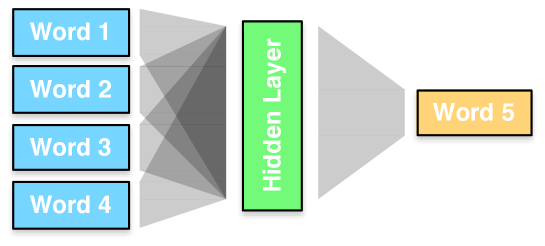
Figure 13.10: Sketch of a neural language model: We predict a word $w_{i}$ based on its preceding words.

Representing Words

We are immediately faced with a difficult question: How do we represent words? Nodes in a neural network carry real-numbered values, but words are discrete items out of a very large vocabulary. We cannot simply use token IDs, since the neural network will assume that token 124,321 is very similar to token 124,322 — while in practice these numbers are completely arbitrary. The same arguments applies to the idea of using bit encoding for token IDs. The words $(1,1,1,1,0,0,0,0)^{T}$ and $(1,1,1,1,0,0,0,1)^{T}$ have very similar encodings but may have nothing to do with each other. While the idea of using such bit vectors is occasionally explored, it does not appear to have any benefits over what we consider next.

Instead, we will represent each word with a high-dimensional vector, one dimension per word in the vocabulary, and the value 1 for the dimension that matches the word, and 0 for the rest. The type of vectors are called one hot vector. For instance:

• dog = $(0,0,0,0,1,0,0,0,0,...)^{T}$

• cat = $(0,0,0,0,0,0,0,1,0,...)^{T}$

• eat = $(0,1,0,0,0,0,0,0,0,...)^{T}$

These are very large vectors, and we will continue to wrestle with the impact of this choice to represent words. One stopgap is to limit the vocabulary to the most frequent, say, 20,000 words, and pool all the other words in an other token. We could also use word classes (either automatic clusters or linguistically motivated classes such as part-of-speech tags) to reduce the dimensionality of the vectors. We will revisit the problem of large vocabularies later.

To pool evidence between words, we introduce another layer between the input layer and the hidden layer. In this layer, each context word is individually projected into a lower dimensional space. We use the same weight matrix for each of the context words, thus generating a continuous space representation for each word, independent of its position in the conditioning context. This representation is commonly referred to as word embedding.

Words that occur in similar contexts should have similar word embeddings. For instance, if the training data for a language model frequently contains the n-grams

• but the cute dog jumped

• but the cute cat jumped

• child hugged the cat tightly

• child hugged the dog tightly

• like to watch cat videos

• like to watch dog videos

then the language model would benefit from the knowledge that dog and cat occur in similar contexts and hence are somewhat interchangeable. If we like to predict from a context where dog occurs but we have seen this context only with the word cat, then we would still like to treat this as positive evidence. Word embeddings enable generalizing between words (clustering) and hence having robust predictions in unseen contexts (back-off).

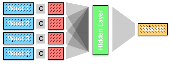
Figure 13.11: Full architecture of a feed-forward neural network language model. Context words ($w_{i-4},w_{i-3},w_{i-2},w_{i-1}$) are represented in a one-hot vector, then projected into continuous space as word embeddings (using the same weight matrix $C$ for all words). The predicted word is computed as a one-hot vector via a hidden layer.

Neural Network Architecture

See Figure 13.11 for a visualization of the architecture the fully fledged feed forward neural network language model, consisting of the context words as one-hot-vector input layer, the word embedding layer, the hidden layer and predicted output word layer.

The context words are first encoded as one-hot vectors. These are then passed through the embedding matrix $C$, resulting in a vector of floating point numbers, the word embedding. This embedding vector has typically in the order of 500 or 1000 nodes. Note that we use the same embedding matrix $C$ for all the context words.

Also note that mathematically there is not all that much going on here. Since the input to the multiplication to the matrix $C$ is a one hot vector, most of the input values to the matrix multiplication are zeros. So, practically, we are selecting the one column in the matrix that corresponds to the input word ID. Hence, there is no use for an activation function here. In a way, the embedding matrix a lookup table $C(w_{j})$ for word embeddings, indexed by the word ID $w_{j}$.

$$C(w_{j})=C\;w_{j}$$ (13.55)

Mapping to the hidden layer in the model requires concatenation of all context word embeddings $C(w_{j})$ as input to a typical feed-forward layer, say, using tanh as activation function.

$$h=\text{tanh}\Big{(}b_{h}+\sum_{j}H_{j}C(w_{j})\Big{)}$$ (13.56)

The output layer is interpreted as a probability distribution over words. As before, first the linear combination $s_{i}$ of weights $w_{ij}$ and hidden node values $h_{j}$ is computed for each node $i$.

$$s=W\;h$$ (13.57)

To ensure that it is indeed a proper probability distribution, we use the softmax activation function to ensure that all values add up to one.

$$p_{i}=\text{softmax}(s_{i},\vec{s})=\frac{e^{s_{i}}}{\sum_{j}e^{s_{j}}}$$ (13.58)

What we described here is close to the neural probabilistic language model proposed by Bengio et al. (2003). This model had one more twist, it added direct connections of the context word embeddings to the output word. So, Equation 13.57 is replaced by

$$s=W\;h+\sum_{j}U\;C(w_{j})$$ (13.59)

Their paper reports that having such direct connections from context words to output words speeds up training, although does not ultimately improve performance. We will encounter the idea of short-cutting hidden layers again a bit later when we discuss deeper models with more hidden layers. They are also called residual connections, skip connections, or even highway connections.

Training

We train the parameters of a neural language model (word embedding matrix, weight matrices, bias vectors) by processing all the n-grams in the training corpus. For each n-gram, we feed the context words into the network and match the network’s output against the one-hot vector of the correct word to be predicted. Weights are updated using back-propagation (we will go into details in the next section).

Language models are commonly evaluated by perplexity, which is related to the probability given to proper English text. A language model that likes proper English is a good language model. Hence, the training objective for language models is to increase the likelihood of the training data.

During training, given a context $\text{\bf x}=(w_{n-4},w_{n-3},w_{n-2},w_{n-1})$, we have the correct value for the 1-hot vector $\vec{y}$. For each training example $(\text{\bf x},\vec{y})$, likelihood is defined as

$$L({\bf x},\vec{y};W)=-\sum_{k}y_{k}\;\text{log}\;p_{k}$$ (13.60)

Note that only one value $y_{k}$ is 1, the others are 0. So this really comes down to the probability $p_{k}$ given to the correct word $k$. Defining likelihood this way allows us to update all weights, also the one that lead to the wrong output words.

Word Embedding

Before we move on, it is worth reflecting the role of word embeddings in neural machine translation and many other natural language processing tasks. We introduced them here as compact encoding of words in relatively high-dimensional space, say 500 or 1000 floating point numbers. In the field of natural language processing, at the time of this writing, word embeddings have acquired the reputation of almost magical quality.

Consider the role they play in the neural language language that we just described. They represent context words to enable prediction the next word in a sequence.

Recall part of our earlier example:

• but the cute dog jumped

• but the cute cat jumped

Since dog and cat occur in similar contexts, their influence on predicting the word jumped should be similar. It should be different from words such as dress which is unlikely to trigger the completion jumped. The idea that words that occur in similar contexts are semantically similar is a powerful idea in lexical semantics.

At this point in the argument, researchers love to cite John Rupert Firth:

You shall know a word by the company it keeps.

Or, as Ludwig Wittgenstein put it a bit more broadly:

The meaning of a word is its use.

Meaning and semantics are quite difficult concepts with largely unresolved definition. The idea of distributional lexical semantics is to define word meaning by their distributional properties, i.e., in which contexts they occur. Words that occur in similar contexts (dog and cat) should have similar representations. In vector space models, such as the word embeddings that we use here, similarity can be measured by a distance function, e.g., the cosine distance — the angle between the vectors.

If we project the high-dimensional word embeddings down to two dimensions, we can visualize word embeddings as shown in Figure 13.12. In this figure, words that are similar (drama, theater, festival) are clustered together.

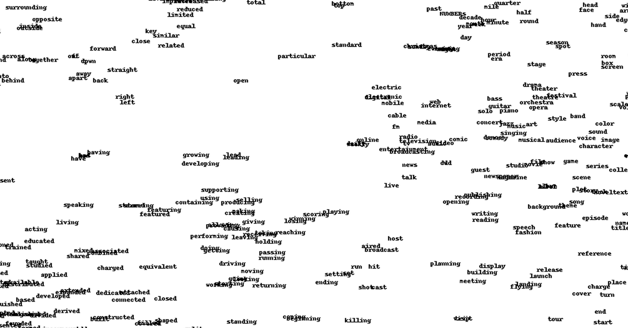
Figure 13.12: Word embeddings projected into 2D. Semantically similar words occur close to each other.

But why stop there? We would like to have semantic representations so we can carry out semantic inference such as

• queen = king + (woman – man)

• queens = queen + (kings – king)

Indeed there is some evidence that word embedding allow just that (Mikolov et al., 2013). However, we better stop here and just note that word embeddings are a crucial tool in neural machine translation.

Efficient Inference and Training

Training a neural language model is computationally expensive. For billion word corpora, even with the use of GPUs, training takes several days with modern compute clusters. Even using a neural language model as a scoring component in statistical machine translation decoding requires a lot of computation. We could restrict its use only to re-ranking n-best lists or lattices, or consider more efficient methods for inference and training.

Caching for Inference

However, with a few considerations, it is actually possible to use this neural language model within the decoder.

• Word embeddings are fixed for the words, so do not actually need to carry out the mapping from one-hot vectors to word embeddings, but just store them beforehand.

• The computation between embeddings and the hidden layer can be also partly carried out offline. Note that each word can occur in one of the 4 slots for conditioning context (assuming a 5-gram language model). For each of the slots, we can pre-compute the matrix multiplication of word embedding vector and the corresponding submatrix of weights. So, at run time, we only have to sum up these pre-computations at the hidden layer and apply the activation function.

• Computing the value for each output node is insanely expensive, since there are as many output nodes as vocabulary items. However, we are interested only in the score for a given word that was produced by the translation model. If we only compute its node value, we have a score that we can use.

The last point requires a longer discussion. If we compute the node value only for the word that we want to score with the language model, we are missing an important step. To obtain a proper probability, we need to normalize it, which requires the computation of the values for all the other nodes.

We could simply ignore this problem and use the scores at face value. More likely words given a context will get higher scores than less likely words, and that is the main objective. But since we place no constraints on the scores, we may work with models where some contexts give high scores to many words, while some contexts do not give preference for any.

It would be great, if the node values in the final layer were already normalized probabilities. There are methods to enforce this during training. Let us first discuss training in detail, and then move to these methods in Section 13.4.3.

Noise Contrastive Estimation

We discussed earlier the problem that computing probabilities with a neural language model is very expensive due to the need to normalize the output node values $y_{i}$ using the softmax function. This requires computing values for all output nodes, even if we are only interested in the score for a particular n-gram. To overcome the need for this explicit normalization step, we would like to train a model that already has $y_{i}$ values that are normalized.

One way is to include the constraint that the normalization factor $Z(x)=\sum_{j}e^{s_{j}}$ is close to 1 in the objective function. So, instead of the just the simple likelihood objective, we may include the L2 norm of the log of this factor. Note that if $\text{log}\;Z(x)\simeq 0$, then $Z(x)\simeq 1$.

$$L({\bf x},\vec{y};W)=-\sum_{k}y_{k}\;\text{log}\;p_{k}-\alpha\;\text{log}^{2}\;Z(x)$$ (13.61)

Another way to train a self-normalizing model is called noise contrastive estimation. The main idea is to optimize the model so that it can separate correct training examples from artificially created noise examples. This method needs less computation during training, since it does not require the computation of all output node values.

Formally, we are trying to learn the model distribution $p_{m}(\vec{y}|{\bf x};W)$. Given a noise distribution $p_{n}(\vec{y}|{\bf x})$ — in our case of language modeling a unigram model $p_{n}(\vec{y})$ is a good choice — we first generate a set of noise examples $U_{n}$ in addition to the correct training examples $U_{t}$. If both sets have the same size $|U_{n}|=|U_{t}|$, then the probability that a given example $({\bf x};\vec{y})\in U_{n}\cup U_{t}$ is predicted to be a correct training example is

$$p(\text{correct}|{\bf x},\vec{y})=\frac{p_{m}(\vec{y}|{\bf x};W)}{p_{m}(\vec{y}|{\bf x};W)+p_{n}(\vec{y}|{\bf x})}$$ (13.62)

The objective of noise contrastive estimation is to maximize $p(\text{correct}|{\bf x},\vec{y})$ for correct training examples $({\bf x};\vec{y})\in U_{t}$ and to minimize it for noise examples $({\bf x};\vec{y})\in U_{n}$. Using log-likelihood, we define the objective function as

$$L=\frac{1}{2|U_{t}|}\sum_{({\bf x};\vec{y})\in U_{t}}\text{log}\;p(\text{correct}|{\bf x},\vec{y})\;\;+\frac{1}{2|U_{n}|}\sum_{({\bf x};\vec{y})\in U_{n}}\text{log}\;(1-p(\text{correct}|{\bf x},\vec{y}))$$ (13.63)

Returning the the original goal of a self-normalizing model, first note that the noise distribution $p_{n}(\vec{y}|{\bf x})$ is normalized. Hence, the model distribution is encouraged to produce comparable values. If $p_{m}(\vec{y}|{\bf x};W)$ would generally overshoot — i.e., $\sum_{\vec{y}}p_{m}(\vec{y}|{\bf x};W)>1$ then it would also give too high values for noise examples. Conversely, generally undershooting would give too low values to correct translation examples.

Training is faster, since we only need to compute the output node value for the given training and noise examples — there is no need to compute the other values, since we do not normalize with the softmax function.

Given the definition of the training objective $L$, we have now a complete computation graph that we can implement using standard deep learning toolkits, as we have done before. These toolkits compute the gradients $\frac{dL}{dW}$ for all parameters $W$ and use them for parameter updates via gradient descent training (or its variants).

It may not be immediately obvious why optimizing towards classifying correct against noise examples gives rise to a model that also predicts the correct probabilities for n-grams. But this is a variant of methods that are common in statistical machine translation in the tuning phase. MIRA (margin infused relaxation algorithm) and PRO (pairwise ranked optimization) follow the same principle.

Recurrent Neural Language Models

The feed-forward neural language model that we described above is able to use longer contexts than traditional statistical back-off models, since it has more flexible means to deal with unknown contexts. Namely, the use of word embeddings to make use of similar words, and the robust handling of unseen words in any context position. Hence, it is possible to condition on much larger contexts than traditional statistical models. In fact, large models, say, 20-gram models, have been reported to be used.

Alternatively, instead of using a fixed context word window, recurrent neural networks may condition on context sequences of any length. The trick is to re-use the hidden layer when predicting word $w_{n}$ as additional input to predict word $w_{n-1}$.

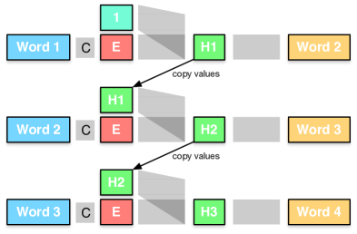
Figure 13.13: Recurrent neural language models: After predicting Word 2 in the context of following Word 1, we re-use this hidden layer (alongside the correct Word 2) to predict Word 3. Again, the hidden layer of this prediction is re-used for the prediction of Word 4.

See Figure 13.13 for an illustration. Initially, the model does not look any different from the feed-forward neural language model that we discussed so far. The inputs to the network is the first word of the sentence $w_{1}$ and a second set of neurons which at this point indicate the start of the sentence. The word embedding of $w_{1}$ and the start-of-sentence neurons first map into a hidden layer $h_{1}$, which is then used to predict the output word $w_{2}$.

This model uses the same architecture as before: Words (input and output) are represented with one-hot vectors; word embeddings and the hidden layer use, say, 500 real valued neurons. We use a sigmoid activation function at the hidden layer and the softmax function at the output layer.

Things get interesting when we move to predicting the third word $w_{3}$ in the sequence. One input is the directly preceding (and now known) word $w_{2}$, as before. However, the neurons in the network that we used to represent start-of-sentence are now filled with values from the hidden layer of the previous prediction of word $w_{2}$. In a way, these neurons encode the previous sentence context. They are enriched at each step with information about a new input word and are hence conditioned on the full history of the sentence. So, even the last word of the sentence is conditioned in part on the first word of the sentence. Moreover, the model is simpler: it has less weights than a 3-gram feed-forward neural language model.

How do we train such a model with arbitrarily long contexts?

One idea: At the initial stage (predicting the second word from the first), we have the same architecture and hence the same training procedure as for feed-forward neural networks. We assess the error at the output layer and propagate updates back to the input layer. We could process every training example this way — essentially by treating the hidden layer from the previous training example as fixed input the current example. However, this way, we never provide feedback to the representation of prior history in the hidden layer.

The back-propagation through time training procedure (see Figure 13.14) unfolds the recurrent neural network over a fixed number of steps, by going back over, say, 5 word predictions. Note that, despite limiting the unfolding to 5 time steps, the network is still able to learn dependencies over longer distances.

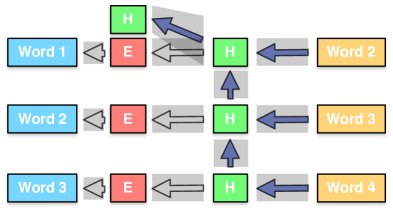
Figure 13.14: Back-propagation through time: By unfolding the recurrent neural network over a fixed number of prediction steps (here: 3), we can derive update formulas based on the training objective of predicting all output words and back-propagation of the error via gradient descent.

Back-propagation through time can be either applied for each training example (here called time step), but this is computationally quite expensive. Each time computations have to be carried out over several steps. Instead, we can compute and apply weight updates in mini-batches (recall Section 13.2.6). First, we process a larger number of training examples (say, 10-20, or the entire sentence), and then update the weights.

Given modern compute power, fully unfolding the recurrent neural network has become more common. While recurrent neural networks have in theory arbitrary length, given a specific training example, its size is actually known and fixed, so we can fully construct the computation graph for each given training example, define the error as the sum of word prediction errors, and then carry out back-propagation over the entire sentence. This does require that we can quickly build computation graphs — so-called dynamic computation graphs — which is currently supported by some toolkits better than others.

Long Short-Term Memory Models

Consider the following step during word prediction in a sequential language model:

After much economic progress over the years, the country $\rightarrow$ has

The directly preceding word country will be the most informative for the prediction of the word has, all the previous words are much less relevant. In general, the importance of words decays with distance. The hidden state in the recurrent neural network will always be updated with the most recent word, and its memory of older words is likely to diminish over time.

But sometimes, more distant words are much more important, as the following example shows:

The country which has made much economic progress over the years still $\rightarrow$ has

In this example, the inflection of the verb have depends on the subject country which is separated by a long subordinate clause.

Recurrent neural networks allow modeling of arbitrarily long sequences. Their architecture is very simple. But this simplicity causes a number of problems.

• The hidden layer plays double duty as memory of the network and as continuous space representation used to predict output words.

• While we may sometimes want to pay more attention to the directly previous word, and sometimes pay more attention to the longer context, there is no clear mechanism to control that.

• If we train the model on long sequences, then any update needs to back propagate to the beginning of the sentence. However, propagating through so many steps raises concerns that the impact of recent information at any step drowns out older information.

The rather confusingly named long short-term memory (LSTM) neural network architecture addresses these issues. Its design is quite elaborate, although it is not very difficult to use in practice.

A core distinction is that the basic building block of LSTM networks, the so-called cell, contains an explicit memory state. The memory state in the cell is motivated by digital memory cells in ordinary computers. Digital memory cells offer operations to read, write, and reset. While a digital memory cell may store just a single bit, a LSTM cell stores a real number.

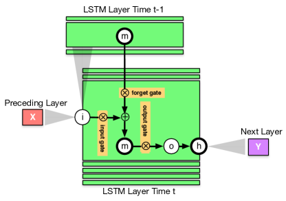
Figure 13.15: A cell in a LSTM neural network. As recurrent neural networks, it receives input from the preceeding layer ($x$) and the hidden layer values from the previous time step $t-1$. The memory state $m$ is updated from the input state $i$ and the previous time’s value of the memory state $m^{t-1}$. Various gates channel information flow in the cell towards the output value $o$.

Furthermore, the read/write/reset operations in a LSTM cell are regulated with a real numbered parameter, which are called gates (see Figure 13.15).

• The input gate parameter regulates how much new input changes the memory state.

• The forget gate parameter regulates how much of the prior memory state is retained (or forgotten).

• The output gate parameter regulates how strongly the memory state is passed on to the next layer.

Formally, marking the input, memory, and output values with the time step $t$, we define the flow of information within a cell as follows.

$$\begin{split}\text{memory}^{t}&=\text{gate}_{\text{input}}\times\text{input}^{t}+\text{gate}_{\text{forget}}\times\text{memory}^{t-1}\\ \text{output}^{t}&=\text{gate}_{\text{output}}\times\text{memory}^{t}\end{split}$$ (13.64)

The hidden node value $h^{t}$ passed on to the next layer is the application of an activation function $f$ to the output value.

$$h^{t}=f(\text{output}^{t})$$ (13.65)

An LSTM layer consists of a vector of LSTM cells, just as traditional layers consist of a vector of nodes. The input to LSTM layer is computed in the same way as the input to a recurrent neural network node. Given the node values for the prior layer $x^{t}$ and the values for the hidden layer from the previous time step $h^{t-1}$, the input value is the typical combination of matrix multiplication with weights $W^{x}$ and $W^{h}$ and an activation function $g$.

$$\text{input}^{t}=g\left(W^{x}x^{t}+W^{h}h^{t-1}\right)$$ (13.66)

But how are the gate parameters set? They actually play a fairly important role. In particular contexts, we would like to give preference to recent input ($\text{gate}_{\text{input}}\simeq 1$), rather retain past memory ($\text{gate}_{\text{forget}}\simeq 1$), or pay less attention to the cell at the current point in time ($\text{gate}_{\text{output}}\simeq 0$). Hence, this decision has to be informed by a broad view of the context.

How do we compute a value from such a complex conditioning context? Well, we treat it like a node in a neural network. For each gate $a\in(\text{input},\text{forget},\text{output})$ we define matrices $W^{xa}$, $W^{ha}$, and $W^{ma}$ to compute the gate parameter value by the multiplication of weights and node values in the previous layer $x^{t}$, the hidden layer $h^{t-1}$ at the previous time step, and the memory states at the previous time step $\text{memory}^{t-1}$, followed by an activation function $h$.

$$\text{gate}_{a}=h\left(W^{xa}x^{t}+W^{ha}h^{t-1}+W^{ma}\text{memory}^{t-1}\right)$$ (13.67)

LSTM are trained the same way as recurrent neural networks, using back-propagation through time or fully unrolling the network. While the operations within a LSTM cell are more complex than in a recurrent neural network, all the operations are still based on matrix multiplications and differentiable activation functions. Hence, we can compute gradients for the objective function with respect to all parameters of the model and compute update functions.

Gated Recurrent Units

LSTM cells add a large number of additional parameters. For each gate alone, multiple weight matrices are added. More parameters lead to longer training times and risk overfitting. As a simpler alternative, gated recurrent units (GRU) have been proposed and used in neural translation models. At the time of writing, LSTM cells seem to make a comeback in neural machine translation, but both are still commonly used.

See Figure 13.16 for an illustration for GRU cells. There is no separate memory state, just a hidden state that serves both purposes. Also, there are only two gates. These gates are predicted as before from the input and the previous state.

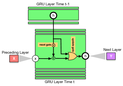
Figure 13.16: Gated Recurrent Unit (GRU): a simplification of long short term memory (LSTM) cells.

$$\text{update}_{t} =g(W_{\text{update}}\;\text{input}_{t}+U_{\text{update}}\;\text{state}_{t-1}+\text{bias}_{\text{update}})$$ (13.68)

$$\text{reset}_{t} =g(W_{\text{reset}}\;\;\;\text{input}_{t}+U_{\text{reset}}\;\;\;\;\text{state}_{t-1}+\text{bias}_{\text{reset}})$$

The first gate is used in the combination of the input and previous state. This is combination is identical to traditional recurrent neural network, except that the previous states impact is scaled by the reset gate. Since the gate’s value is between 0 and 1, this may give preference to the current input.

$$\text{combination}_{t}=f(W\;\text{input}_{t}+U(\text{reset}_{t}\circ\text{state}_{t-1}))$$ (13.69)

Then, the update gate is used for a interpolation of the previous state and the just computed combination. This is done as a weighted sum, where the update gate balances between the two.

$$\text{state}_{t}= (1-\text{update}_{t})\circ\text{state}_{t-1}\;+$$ (13.70)

$$\text{update}_{t}\;\;\;\;\;\;\;\;\;\circ\text{combination}_{t})+\text{bias}$$

In one extreme case, the update gate is 0, and the previous state is passed through directly. In another extreme case, the update gate is 1, and the new state is mainly determined from the input, with as much impact from the previous state as the reset gate allows.

It may seem a bit redundant to have two operations with a gate each that combine prior state and input. However, these play different roles. The first operation yielding $\text{combination}_{t}$ (Equation 13.69) is a classic recurrent neural network component that allows more complex computations in the combination of input and output. The second operation yielding the new hidden state and the output of the unit (Equation 13.70) allows for bypassing of the input, enabling long-distant memory that simply passes through information and, during back-propagation, passes through the gradient, thus enabling long-distance dependencies.

Deep Models

The currently fashionable name deep learning for the latest wave of neural network research has a real motivation. Large gains have been seen in tasks such as vision and speech recognition due to stacking multiple hidden layers together.

More layers allow for more complex computations, just as having sequences of traditional computation components (Boolean gates) allows for more complex computations such as addition and multiplication of numbers. While this has been generally recognized for a long time, modern hardware finally enabled to train such deep neural networks on real world problems. And we learned from experiments in vision and speech that having a handful, and even dozens of layers does give increasingly better quality.

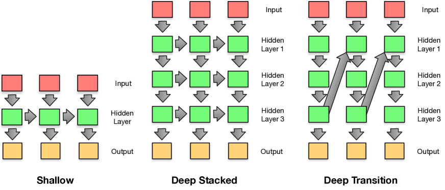
Figure 13.17: Deep recurrent neural networks. The input is passed through a few hidden layers before an output prediction is made. In deep stacked models, the hidden layers are also connected horizontally, i.e., a layer’s values at time step $t$ depends on its value at time step $t-1$ as well as the previous layer at time step $t$. In deep transitional models, the layers at any time step $t$ are sequentially connected and first hidden layer is also informed by the last layer at time step $t-1$.

How does the idea of deep neural networks apply to the sequence prediction tasks common in language? There are several options. Figure 13.17 gives two examples. In shallow neural networks, the input is passed to a single hidden layer, from which the output is predicted. Now, a sequence of hidden layers is used. These hidden layers $h_{t,i}$ may be deeply stacked, so that each layer acts like the hidden layer in the shallow recurrent neural network. Its state is conditioned on its value at the previous time step $h_{t-1,i}$ and the value of previous layer in the sequence $h_{t,i-1}$.

$$h_{t,1} =f_{1}(h_{t-1,1},x_{t})$$ first layer (13.71)

$$h_{t,i} =f_{i}(h_{t-1,i},h_{t,i-1}) i>1$$ for

$$y_{t} =f_{i+1}(h_{t,I}) I$$ prediction from last layer

Or, the hidden layers may be directly connected in deep transitional networks, where the first hidden layer $h_{t,1}$ is informed by the last hidden layer at the previous time step $h_{t-1,I}$, but all other hidden layers are not connected to values from previous time steps.

$$h_{t,1} =f_{1}(h_{t-1,I},x_{t})$$ first layer (13.72)

$$h_{t,i} =f_{i}(h_{t,i-1}) i>1$$ for

$$y_{t} =f_{i+1}(h_{t,I}) I$$ prediction from last layer

In all these equations, the function $f_{i}$ may be a feedforward layer (matrix multiplication plus activation function), an LSTM cell or a GRU cell.

Experiments with using neural language models in traditional statistical machine translation have shown benefits with 3–4 hidden layers (Luong et al., 2015a).

While modern hardware allows training of deep models, they do stretch computational resources to their practical limit. Not only are there more computations in the neural network, convergence of training is typically slower. Adding skip connections (linking the input directly to the output or the final hidden layer) sometimes speeds up training, but we still talking about a several times longer training times than shallow networks.

Further Readings

The first vanguard of neural network research tackled language models. A prominent reference for neural language model is Bengio et al. (2003), who implement an n-gram language model as a feed-forward neural network with the history words as input and the predicted word as output. Schwenk et al. (2006) introduce such language models to machine translation (also called “continuous space language models"), and use them in re-ranking, similar to the earlier work in speech recognition. Schwenk (2007) propose a number of speed-ups. They made their implementation available as a open source toolkit (Schwenk, 2010), which also supports training on a graphical processing unit (GPU) (Schwenk et al., 2012).

By first clustering words into classes and encoding words as pair of class and word-in-class bits, Baltescu et al. (2014) reduce the computational complexity sufficiently to allow integration of the neural network language model into the decoder. Another way to reduce computational complexity to enable decoder integration is the use of noise contrastive estimation by Vaswani et al. (2013), which roughly self-normalizes the output scores of the model during training, hence removing the need to compute the values for all possible output words. Baltescu and Blunsom (2015) compare the two techniques - class-based word encoding with normalized scores vs. noise-contrastive estimation without normalized scores - and show that the letter gives better performance with much higher speed.

As another way to allow straightforward decoder integration, Wang et al. (2013) convert a continuous space language model for a short list of 8192 words into a traditional n-gram language model in ARPA (SRILM) format. Wang et al. (2014) present a method to merge (or “grow") a continuous space language model with a traditional n-gram language model, to take advantage of both better estimate for the words in the short list and the full coverage from the traditional model.

Finch et al. (2012) use a recurrent neural network language model to rescore n-best lists for a transliteration system. Sundermeyer et al. (2013) compare feed-forward with long short-term neural network language models, a variant of recurrent neural network language models, showing better performance for the latter in a speech recognition re-ranking task. Mikolov (2012) reports significant improvements with reranking n-best lists of machine translation systems with a recurrent neural network language model.

Neural language model are not deep learning models in the sense that they use a lot of hidden layers. Luong et al. (2015a) show that having 3-4 hidden layers improves over having just the typical 1 layer.

Language Models in Neural Machine Translation: Traditional statistical machine translation models have a straightforward mechanism to integrate additional knowledge sources, such as a large out of domain language model. It is harder for end-to-end neural machine translation. Gülçehre et al. (2015) add a language model trained on additional monolingual data to this model, in form of a recurrently neural network that runs in parallel. They compare the use of the language model in re-ranking (or, re-scoring) against deeper integration where a gated unit regulates the relative contribution of the language model and the translation model when predicting a word.

Neural Translation Models

We are finally prepared to look at actual translation models. We have already done most of the work, however, since the most commonly used architecture for neural machine translation is a straightforward extension of neural language models with one refinement, an alignment model.

Encoder-Decoder Approach

Our first stab at a neural translation model is a straightforward extension of the language model. Recall the idea of a recurrent neural network to model language as a sequential process. Given all previous words, such a model predicts the next word. When we reach the end of the sentence, we now proceed to predict the translation of the sentence, one word at a time.

See Figure 13.18 for an illustration. To train such a model, we simply concatenate the input and output sentences and use the same method as to train a language model. For decoding, we feed in the input sentence, and then go through the predictions of the model until it predicts an end of sentence token.

Figure 13.18: Sequence-to-sequence encoder-decoder model: Extending the language model, we concatenate the English input sentence the house is big with the German output sentence das Haus ist groß. The first dark green box (after processing the end-of-sentence token $<$/s$>$) contains the embedding of the entire input sentence .

How does such a network work? Once processing reaches the end of the input sentence (having predicted the end of sentence marker $<$/s$>$), the hidden state encodes its meaning. In other words, the vector holding the values of the nodes of this final hidden layer is the input sentence embedding. This is the encoder phase of the model. Then this hidden state is used to produce the translation in the decoder phase.

Clearly, we are asking a lot from the hidden state in the recurrent neural network here. During encoder phase, it needs to incorporate all information about the input sentence. It cannot forget the first words towards the end of the sentence. During the decoder phase, not only does it need to have enough information to predict each next word, there also needs to be some accounting for what part of the input sentence has been already translated, and what still needs to be covered.

In practice, the proposed models works reasonable well for short sentences (up to, say, 10–15 words), but fails for long sentences. Some minor refinements to this model have been proposed, such using the sentence embedding state as input to all hidden states of the decoder phase of the model. This makes the decoder structurally different from the encoder and reduces some of the load from the hidden state during decoding, since it does not need to remember anymore the input. Another idea is to reverse the order of the output sentence, so that the last words of the input sentences are close to the last words of the output sentence.

However, in the following section, we will embark on a more significant improvement of the model, by explicitly modelling alignment of output words to input words.

Adding an Alignment Model

At the time of writing, the state of the art in neural machine translation is a sequence-to-sequence encoder-decoder model with attention. That is a mouthful, but it is essentially the model we just described in the previous section, with a explicitly alignment mechanism. In the deep learning world, this alignment is called attention, we are using the words alignment and attention interchangeable here.

Since the attention mechanism does add a bit of complexity to the model, we are now slowly building up to it, by first taking a look at the encoder, then the decoder, and finally the attention mechanism.

Encoder

The task of the encoder is to provide a representation of the input sentence. The input sentence is a sequence of words, for which we first consult the embedding matrix. Then, as in the basic language model described previously, we process these words with a recurrent neural network. This results in hidden states that encode each word with its left context, i.e., all the preceding words. To also get the right context, we also build a recurrent neural network that runs right-to-left, or more precisely, from the end of the sentence to the beginning.

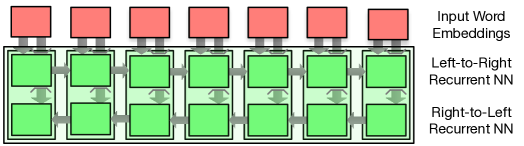
Figure 13.19: Neural machine translation model, part 1: input encoder. It consists of two recurrent neural networks, running right to left and left to right (bidrectional recurrent neural network). The encoder states are the combination of the two hidden states of the recurrent neural networks.

Figure 13.19 illustrates the model. Having two recurrent neural networks running in two directions is called a bidirectional recurrent neural network. Mathematically, the encoder consists of the embedding lookup for each input word $x_{j}$, and the mapping that steps through the hidden states $\overleftarrow{h_{j}}$ and $\overleftarrow{h_{j}}$

$$\overleftarrow{h_{j}}=f(\overleftarrow{h_{j+1}},\bar{E}\;x_{j})$$ (13.73)

$$\overrightarrow{h_{j}}=f(\overrightarrow{h_{j-1}},\bar{E}\;x_{j})$$ (13.74)

In the equation above, we used a generic function $f$ for a cell in the recurrent neural network. This function may be a typical feed-forward neural network layer — such as $f(x)=\text{tanh}(Ax+b)$ — or the more complex gated recurrent units (GRUs) or long short term memory cells (LSTMs). The original paper proposing this approached used GRUs, but lately LSTMs have become more popular.

Note that we could train these models by adding a step that predicts the next word in the sequence, but we are actually training it in the context of the full machine translation model. Limiting the description to the decoder, its output is a sequence of word representations that concatenate the two hidden states $(\overleftarrow{h_{j}},\overrightarrow{h_{j}})$.

Decoder

The decoder is also a recurrent neural network. It takes some representation of the input context (more on that in the next section on the attention mechanism) and the previous hidden state and output word prediction, and generates a new hidden decoder state and a new output word prediction. See Figure 13.20 for an illustration.

Mathematically, we start with the recurrent neural network that maintains a sequence of hidden states $s_{i}$ which are computed from the previous hidden state $s_{i-1}$, the embedding of the previous output word $Ey_{i-1}$, and the input context $c_{i}$ (which we still have to define).

$$s_{i}=f(s_{i-1},\;Ey_{i-1},c_{i})$$ (13.75)

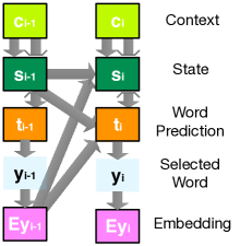
Figure 13.20: Neural machine translation model, part 2: output decoder. Given the context from the input sentence, and the embedding of the previously selected word, new decoder states and word predictions are computed.

Again, there are several choices for the function $f$ that combines these inputs to generate the next hidden state: linear transforms with activation function, GRUs, LSTMs, etc. Typically, the choice here matches the encoder. So, if we use LSTMs for the encoder, then we also use LSTMs for the decoder.

From the hidden state. we now predict the output word. This prediction takes the form of a probability distribution over the entire output vocabulary. If we have a vocabulary of, say, 50,000 words, then the prediction is a 50,000 dimensional vector, each element corresponding to the probability predicted for one word in the vocabulary.

The prediction vector $t_{i}$ is conditioned on the decoder hidden state $s_{i-1}$ and, again, the embedding of the previous output word $Ey_{i-1}$ and the input context $c_{i}$.

$$t_{i}=\text{softmax}\big{(}W(Us_{i-1}+VEy_{i-1}+Cc_{i})\big{)}$$ (13.76)

Note that we repeat the conditioning on $Ey_{i-1}$ since we use the hidden state $s_{i-1}$ and not $s_{1}$. This separates the encoder state progression from $s_{i-1}$ to $s_{i}$ from the prediction of the output word $t_{i}$.

The softmax is used to convert the raw vector into a probability distribution, where the sum of all values is 1. Typically, the highest value in the vector indicates the output word token $y_{i}$. Its word embedding $Ey_{i-1}$ informs the next time step of the recurrent neural network.

During training, the correct output word $y_{i}$ is known, so training proceeds with that word. The training objective is to give as much probability mass as possible to the correct output word. The cost function that drives training is hence the negative log of the probability given to the correct word translation.

$$\text{cost}=-\text{log}\;t_{i}[y_{i}]$$ (13.77)

Ideally, we want to give the correct word the probability 1, which would mean a negative log probability of 0, but typically it is a lower probability, hence a higher cost. Note that the cost function is tied to individual words, the overall sentence cost is the sum of all word costs.

During inference on a new test sentence, we typically chose the word $y_{i}$ with the highest value in $t_{i}$ use its embedding $Ey_{i}$ for the next steps. But we will also explore beam search strategies where the next likely words are selected as $y_{i}$, creating a different conditioning context for the next words. More on that later.

Attention Mechanism

We currently have two loose ends. The decoder gave us a sequence of word representations $h_{j}=(\overleftarrow{h_{j}},\overrightarrow{h_{j}})$ and the decoder expects a context $c_{i}$ at each step $i$. We now describe the attention mechanism that ties these ends together.

The attention mechamism is hard to visualize using our typical neural network graphs, but Figure 13.21 gives at least an idea what the input and output relations are. The attention mechanism is informed by all input word representations $(\overleftarrow{h_{j}},\overrightarrow{h_{j}})$ and the previous hidden state of the decoder $s_{i-1}$, and it produces a context state $c_{i}$.

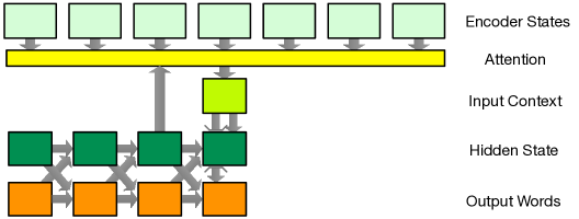
Figure 13.21: Neural machine translation model, part 3: attention model. Associations are computed between the last hidden state of the decoder and the word representations (encoder states). These associations are used to compute a weighted sum of encoder states.

The motivation is that we want to compute an association between the decoder state (which contains information where we are in the output sentence production) and each input word. Based on how strong this association is, or in other words how relevant each particular input word is to produce the next output word, we want to weight the impact of its word representation.

Mathematically, we first compute this association with a feedforward layer (using weight vectors $w^{a}$, $u^{a}$ and bias value $b^{a}$)

$$a(s_{i-1},h_{j})={w^{a}}^{T}s_{i-1}+{u^{a}}^{T}h_{j}+b^{a}$$ (13.78)

The output of this computation is a scalar value, indicating how important input word $j$ is to produce output word $i$.

We normalize this attention value, so that the attention values across all input words $j$ add up to one, using the softmax.

$$\alpha_{ij}=\frac{\text{exp}(a(s_{i-1},h_{j}))}{\sum_{k}\text{exp}(a(s_{i-1},h_{k}))}$$ (13.79)

Now we use the normalized attention value to weigh the contribution of the input word representation $h_{j}$ to the context vector $c_{i}$ and we are done.

$$c_{i}=\sum_{j}\alpha_{ij}h_{j}$$ (13.80)

Simply adding up word representation vectors (weighted or not) may at first seem an odd and simplistic thing to do. But it is very common practice in deep learning for natural language processing. Researchers have no qualms about using sentence embeddings that are simply the sum of word embeddings and other such schemes.

Training

With the complete model in hand, we can now take a closer look at training. One challenge is that the number of steps in the decoder and the number of steps in the encoder varies with each training example. Sentence pairs consist of sentences of different length, so we cannot have the same computation graph for each training example but instead have to dynamically create the computation graph for each of them. This technique is called unrolling the recurrent neural networks, and we already discussed it with regard to language models (recall Section 13.4.4).

The fully unrolled computation graph for a short sentence pair is shown in Figure 13.22. Note a couple of things. The error computed from this one sentence pair is the sum of the errors computed for each word. When proceeding to the next word prediction, we use the correct word as conditioning context for the decoder hidden state and the word prediction. Hence, the training objective is based on the probability mass given to the correct word, given a perfect context. There have been some attempts to use different training objectives, such as the bleu score, but they have not yet been shown to be superior.

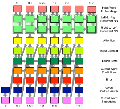
Figure 13.22: Fully unrolled computation graph for training example with 7 input tokens $<$s$>$ the house is big $<$/s$>$ and 6 output tokens das Haus is groß$<$/s$>$. The cost function (error) is computed for each output word individually, and summed up across the sentence. When walking through the deocder states, the correct previous output words are used as conditioning context.

Practical training of neural machine translation models requires GPUs which are well suited to the high degree of parallelism inherent in these deep learning models (just think of the many matrix multiplications). To increase parallelism even more, we process several sentence pairs (say, 100) at once. This implies that we increase the dimensionality of all the state tensors.

To given an example. We represent each input word in specific sentence pair with a vector $h_{j}$. Since we already have a sequence of input words, these are lined up in a matrix. When we process a batch of sentence pairs, we again line up these matrices into a 3-dimensional tensor.

Similarly, to give another example, the decoder hidden state $s_{i}$ is a vector for each output word. Since we process a batch of sentences, we line up their hidden states into a matrix. Note that in this case it is not helpful to line up the states for all the output words, since the states are computed sequentially.

Recall the first computation of the attention mechanism

$$a(s_{i-1},h_{j})=W^{a}s_{i-1}+U^{a}h_{j}+b^{a}$$ (13.81)

We can pass this computation to the GPU with a matrix of encoder states $s_{i-1}$ and a 3-dimensional tensor of input encodings $h_{j}$, resulting in a matrix of attention values (one dimension for the sentence pairs, one dimension for the input words). Due to the massive re-use of values in $W^{a}$, $U^{a}$, and $b^{a}$ as well as the inherent parallelism of this computation, GPUs can show their true power.

You may feel that we just created a glaring contradiction. First, we argued that we have to process one training example at a time, since sentence pairs typically have different length, and hence computation graphs have different size. Then, we argued for batching, say, 100 sentence pairs together to better exploit parallelism. These are indeed conflicting goals.

See Figure 13.23. When batching training examples together, we have to consider the maximum sizes for input and output sentences in a batch and unroll the computation graph to these maximum sizes. For shorter sentences, we fill the remaining gaps with non-words and keep track of where the valid data is with a mask. This means, for instance, that we have to ensure that no attention is given to words beyond the length of the input sentence, and no errors and gradient updates are computed from output words beyond the length of the output sentence.

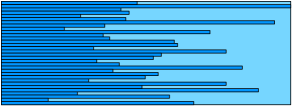
$\Rightarrow$

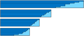
Figure 13.23: To make better use of parallelism in GPUs, we process a batch of training examples (sentence pairs) at a time. Converting a batch of training examples into a set of mini batches that have similar length. This wastes less computation on filler words (light blue).

To avoid wasted computations on gaps, a nice trick is to sort the sentence pairs in the batch by length and break it up into mini-batches of similar length.

To summarize, training consists of the following steps

• Shuffle the training corpus (to avoid undue biases due to temporal or topical order)

• Break up the corpus into maxi-batches

• Break up each maxi-batch into mini-batches

• Process each mini-batch, gather gradients

• Apply all gradients for a maxi-batch to update the parameters

Typically, training neural machine translation models takes about 5–15 epochs (passes through entire training corpus). A common stopping criteria is to check progress of the model on a validation set (that is not part of the training data) and halt when the error on the validation set does not improve. Training longer would not lead to any further improvements and may even degrade performance due to overfitting.

Beam Search

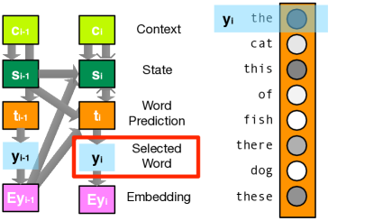
Figure 13.24: Elementary decoding step: The model predicts a word prediction probability distribution. We select the most likely word (the). Its embedding is part of the conditioning context for the next word prediction (and decoder state).

Translating with neural translation models proceeds one step at a time. At each step, we predict one output word. In our model, we first compute a probability distribution over all words. We then pick the most likely word and move to the next prediction step. Since the model is conditioned on the previous output word (recall Equation 13.75), we use its word embedding in the conditioning context for the next step.

See Figure 13.24 for an illustration. At each time step, we obtain a probability distribution over words. In practice, this distribution is most often quite spiked, only few words — or maybe even just one word — amass almost all of the probability. In the example, the word the received the highest probability, so we pick it as the output word.

Input Sentence
ich glaube aber auch , er ist clever genug um seine Aussagen vage genug zu halten , so dass sie auf verschiedene Art und Weise interpretiert werden können .

Output Word Predictions
Best Alternatives but (42.1%) however (25.3%), I (20.4%), yet (1.9%), and (0.8%), nor (0.8%), … I (80.4%) also (6.0%), , (4.7%), it (1.2%), in (0.7%), nor (0.5%), he (0.4%), … also (85.2%) think (4.2%), do (3.1%), believe (2.9%), , (0.8%), too (0.5%), … believe (68.4%) think (28.6%), feel (1.6%), do (0.8%), … he (90.4%) that (6.7%), it (2.2%), him (0.2%), … is (74.7%) ’s (24.4%), has (0.3%), was (0.1%), … clever (99.1%) smart (0.6%), … enough (99.9%) to (95.5%) about (1.2%), for (1.1%), in (1.0%), of (0.3%), around (0.1%), … keep (69.8%) maintain (4.5%), hold (4.4%), be (4.2%), have (1.1%), make (1.0%), … his (86.2%) its (2.1%), statements (1.5%), what (1.0%), out (0.6%), the (0.6%), … statements (91.9%) testimony (1.5%), messages (0.7%), comments (0.6%), … vague (96.2%) v@@ (1.2%), in (0.6%), ambiguous (0.3%), … enough (98.9%) and (0.2%), … so (51.1%) , (44.3%), to (1.2%), in (0.6%), and (0.5%), just (0.2%), that (0.2%), … they (55.2%) that (35.3%), it (2.5%), can (1.6%), you (0.8%), we (0.4%), to (0.3%), … can (93.2%) may (2.7%), could (1.6%), are (0.8%), will (0.6%), might (0.5%), … be (98.4%) have (0.3%), interpret (0.2%), get (0.2%), … interpreted (99.1%) interpre@@ (0.1%), constru@@ (0.1%), … in (96.5%) on (0.9%), differently (0.5%), as (0.3%), to (0.2%), for (0.2%), by (0.1%), … different (41.5%) a (25.2%), various (22.7%), several (3.6%), ways (2.4%), some (1.7%), … ways (99.3%) way (0.2%), manner (0.2%), … . (99.2%) </s> (0.2%), , (0.1%), … </s> (100.0%)

Figure 13.25: Word predictions of the neural machine translation model. Frequently, most of the probability mass is given to the top choice, but semantically related words may rank high, e.g., believe (68.4%) vs. think (28.6%). The subword units interpre@@ are explain in Section 13.6.2.

A real example of how a neural machine translation model translates a German sentence into English is shown in Figure 13.25. The model tends to give most, if not almost all, probability mass to the top choice, but the sentence translation also indicates word choice ambiguity, such as believe (68.4%) vs. think (28.6%) or different (41.5%) vs. various (22.7%). There is also ambiguity about grammatical structure, such as if the sentence should start with the discourse connective but (42.1%) or the subject I (20.4%).

This process suggests that we perform 1-best greedy search. This makes us vulnerable to the so-called garden-path problem. Sometimes we follow a sequence of words and realize too late that we made a mistake early on. In that case, the best sequence consists of less probable words initially which are redeemed by subsequent words in the context of the full output. Consider the case of having to produce an idiomatic phrase that is non-compositional. The first words of these phrases may be really odd word choices by themselves (e.g., piece of cake for easy). Only once the full phrase is formed, their choice is redeemed.

Note that we are faced with the same problem in traditional statistical machine translation models — arguable even more so there since we rely on sparser contexts when making predictions for the next words. Decoding algorithms for these models keep a list of the n-best candidate hypotheses, expand them and keep the n-best expanded hypotheses. We can do the same for neural translation models.

When predicting the first word of the output sentence, we keep a beam of the top $n$ most likely word choices. They are scored by their probability. Then, we use each of these words in the beam in the conditioning context for the next word. Due to this conditioning, we make different word predictions for each. We now multiply the score for the partial translation (at this point just the probability for the first word), and the probabilities from its word predictions. We select the highest scoring word pairs for the next beam. See Figure 13.26 for an illustration.

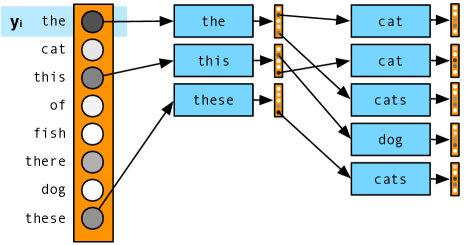
Figure 13.26: Beam search in neural machine translation. After committing to a short list of specific output words (the beam), new word predictions are made for each. These differ since the committed output word is part of the conditioning context to make predictions.

This process continues. At each time step, we accumulate word translation probabilities, giving us scores for each hypothesis. A sentence translation is complete, when the end of sentence token is produced. At this point, we remove the completed hypothesis from the beam and reduce beam size by 1. Search terminates, when no hypotheses are left in the beam.

Search produces a graph of hypotheses, as shown in Figure 13.27. It starts with the start of sentence symbol $<$s$>$ and its paths terminate with the end of sentence symbol $<$/s$>$. Given the compete graph, the resulting translations can be obtained by following the back-pointers. The complete hypothesis (i.e., one that ended with a $<$/s$>$ symbol) with the highest score points to the best translation.

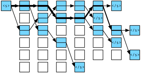
Figure 13.27: Search graph for beam search decoding in neural translation models. At each time step, the $n=6$ best partial translations (called hypotheses) are selected. An output sentence is complete when the end of sentence token $<$/s$>$ is predicted. We reduce the beam after that and terminate when $n$ full sentence translations are completed. Following the back-pointers from the end of sentence tokens allows us to read them off. Empty boxes represent hypotheses that are not part of any complete path.

When choosing among the best paths, we score each with the product of its word prediction probabilities. In practice, we get better results when we normalize the score by the output length of a translation, i.e., divide by the number of words. We carry out this normalization after search is completed. During search, all translations in a beam have the same length, so the normalization would make no difference.

Note that in traditional statistical machine translation, we were able to combine hypotheses if they share the same conditioning context for future feature functions. This not possible anymore for recurrent neural networks since we condition on the entire output word sequence from the beginning. As a consequence, the search graph is generally less diverse than search graphs in statistical machine translation models. It is really just a search tree where the number of complete paths is the same as the size of the beam.

Further Readings

The attention model has its roots in a sequence-to-sequence model. Cho et al. (2014) use recurrent neural networks for the approach. Sutskever et al. (2014) use a LSTM (long short-term memory) network and reverse the order of the source sentence before decoding.

The seminal work by Bahdanau et al. (2015) adds an alignment model (so called “attention mechanism") to link generated output words to source words, which includes conditioning on the hidden state that produced the preceding target word. Source words are represented by the two hidden states of recurrent neural networks that process the source sentence left-to-right and right-to-left. Luong et al. (2015b) propose variants to the attention mechanism (which they call “global" attention model) and also a hard-constraint attention model (“local" attention model) which is restricted to a Gaussian distribution around a specific input word.

To explicitly model the trade-off between source context (the input words) and target context (the already produced target words), Tu et al. (2016a) introduce an interpolation weight (called “context gate") that scales the impact of the (a) source context state and (b) the previous hidden state and the last word when predicting the next hidden state in the decoder.

Tu et al. (2017) augment the attention model with a reconstruction step. The generated output is translated back into the input language and the training objective is extended to not only include the likelihood of the target sentence but also the likelihood to the reconstructed input sentence.

Refinements

The previous section gave a comprehensive description of the currently most commonly used basic neural translation model architecture. It performs fairly well out of the box for many language pairs. Since its conception, a number of refinements have been proposed. We will describe them in this section.

Some of the refinements are fairly general, some target particular use cases or data conditions. To given one example, the best performing system at the recent WMT 2017 evaluation campaign used ensemble decoding (Section 13.6.1), byte pair encoding to address large vocabularies (Section 13.6.2), added synthetic data derived from monolingual target side data (Section 13.6.3) , and used deeper models (Section 13.6.4).

Ensemble Decoding

A common technique in machine learning is to not just build one system for your problem, but multiple ones and then combine them. This is called an ensemble of systems. It is such a successful strategy that various methods have been proposed to systematically build alternative systems, for instance by using different features or different subsets of the data. For neural networks, one straightforward way is to use different initializations or stop at different points in the training process.

Why does it work? The intuitive argument is that each system makes different mistakes. When two systems agree, then they are more likely both right, rather than both make the same mistake. One can also see the general principle at play in human behavior, such as setting up committees to make decisions or the democratic voting in elections.

Applying ensemble methods to our case of neural machine translation, we have to address two sub-problems: (1) generating alternate systems, and (2) combining their output.

Generating Alternative Systems

See Figure 13.28 for an illustration of two methods for the first sub-problem, generating alternative system. When training a neural translation model, we iterate through the training data until some stopping criteria is met. This is typically a lack of improvements of the cost function applied to a validation set (measured in cross-entropy), or the translation performance on that validation set (measured in bleu).

Checkpoint ensemble	Multi-run ensemble

Figure 13.28: Two methods to generate alternative systems for ensembling: Checkpoint ensembling uses model dumps from various stages of the training process, while multi-run ensembling starts independent training runs with different initial weights and order of the training data.

During training, we dump out the model at fixed intervals (say, every 10,000 iteration of batch processing). Once training is completed, we can look back at the performance of the model these different stages. We then pick the, say, 4 models with the best performance (typically translation quality measured in bleu). This is called checkpoint ensembling since we select the models at different checkpoints in the training process.

Multi-run ensembling requires building systems in completely different training runs. As mentioned before, this can be accomplished by using different random initialization of weights, which leads training to seek out different local optima. We also randomly shuffle the training data, so using different random order will also lead to different training outcomes.

Multi-run ensembling usually works a good deal better, but it is also computationally much more expensive. Note that multi-run ensembling can also build on checkpoint ensembling. Instead of combining the end points of training, we first apply checkpoint ensembling to each run, and then combine those ensembles.

Combine System Output

Neural translation models allow the combination of several systems fairly deeply. Recall that the model first predicts a probability distribution over possible output words, and then commits to one of the words. This is where we combine the different trained models. Each model predicts a probability distribution and we then combine their predictions. The combination is done by simple averaging over the distributions. The averaged distribution is then the basis for selecting an output word.

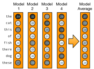
Figure 13.29: Combining predictions from a ensemble of models: Each model independently predicts a probability distribution over output words, which are averaged into a combined distribution.

See Figure 13.29 for an illustration. There may be some benefit to weighing the different systems differently, although in our way of generating them, they will all have very similar quality, so this is not typically done.

Reranking with Right-to-Left Decoding

One more tweak on the idea of ensembling: Instead of building multiple systems with different random initialization, we can also build one set of system as before, and then a second set of system where we reverse the order of the output sentences. The second set of systems are called right-to-left systems, although arguably this is not a good name since it makes no sense for languages such as Arabic or Hebrew where the normal writing order is right to left.

The deep integration we described just above does not work anymore for the combination of left-to-right and right-to-left systems, since they produce output in different order. So, we have to resort to reranking. This involves several steps:

• Use an ensemble of left-to-right systems to generate an n-best list of candidate translations for each input sentence.

• Score each candidate translation with the individual left-to-right and right-to-left systems.

• Combine the scores (simple average) of the different models for each candidate, select the candidate with the best score for each input sentence.

Scoring a given candidate translation with a right-to-left system does require the require forced decoding, a special mode of running inference on an input sentence, but predicting a given output sentence. This mode is actually much closer to training (where also an output translation is given) the regular inference.

Large Vocabularies

Zipf’s law tells us that words in a language are very unevenly distribution. So, there is always a large tail of rare words. New words come into the language all the time (e.g., retweeting, website, woke), and we also have to deal with a very large inventory of names, including company names (e.g., eBay, Yahoo, Microsoft).

On the other hand, neural methods are not well equipped to deal with such large vocabularies. The ideal representations for neural networks are continuous space vectors. This is why we first convert discrete objects such as words into such word embeddings.

However, ultimately the discrete nature of words shows up. On the input side, we need to train an embedding matrix that maps each word into its embedding. On the output side we predict a probability distribution over all output words. The latter is generally the bigger concern, since the amount of computation involved is linear with the size of the vocabulary, making this a very large matrix operation.

Hence, neural translation models typically restrict the vocabulary to, say, 20,000 to 80,000 words. In initial work on neural machine translation, only the most frequent words were used, and all others represented by a unknown or other tag. The translation of these rare words was handled with a back-off dictionary.

The more common approach today is to break up rare words into subword units. This may seem a bit crude but is actually very similar to standard approaches in statistical machine translation to handle compounds (recall website $\rightarrow$ web + site) and morphology (unfollow $\rightarrow$ un + follow, convolutions $\rightarrow$ convolution + s). It is even a decent approach to the problem of transliteration of names which are traditionally handled by a sub-modular letter translation component.

A popular method to create an inventory of subword units and legitimate words is byte pair encoding. This method is trained on the parallel corpus. First, the words in the corpus are split into characters (marking original spaces with a special space character). Then, the most frequent pair of characters is merged (in English, this may be t and h into th). This step is repeated for a fixed given number of times. Each of these steps increases the vocabulary by one, beyond the original inventory of single characters.

The example mirrors quite well the behavior of the algorithm on real-world data sets. It starts with grouping together with frequent letter combinations (e+r, t+h, c+h) and then joins frequent words (the, in, of). At the end of this process, the most frequent words will emerge as single tokens, while rare words consist of still un-merged subwords. See Figure 13.30 for an example, where subword units are indicated with two “at" symbols (@@). After 49,500 byte pair encoding operations, the vast majority of words are intact, while rarer words are broken up (e.g., critic@@ ises, destabil@@ ising). Sometimes, the split seem to be morphologically motivated (e.g., im@@ pending), but mostly they are not (e.g., stra@@ ined). Note also the decomposition of the relatively rare name Net@@ any@@ ahu.

Obama receives Net@@ any@@ ahu

the relationship between Obama and Net@@ any@@ ahu is not exactly friendly . the two wanted to talk about the implementation of the international agreement and about Teheran ’s destabil@@ ising activities in the Middle East . the meeting was also planned to cover the conflict with the Palestinians and the disputed two state solution . relations between Obama and Net@@ any@@ ahu have been stra@@ ined for years . Washington critic@@ ises the continuous building of settlements in Israel and acc@@ uses Net@@ any@@ ahu of a lack of initiative in the peace process . the relationship between the two has further deteriorated because of the deal that Obama negotiated on Iran ’s atomic programme . in March , at the invitation of the Republic@@ ans , Net@@ any@@ ahu made a controversial speech to the US Congress , which was partly seen as an aff@@ ront to Obama . the speech had not been agreed with Obama , who had rejected a meeting with reference to the election that was at that time im@@ pending in Israel .

Figure 13.30: Byte pair encoding (BPE) applied to English (model used 49,500 BPE operations). Word splits are indicated with @@. Note that the data is also tokenized and true-cased.

Further Readings

A significant limitation of neural machine translation models is the computational burden to support very large vocabularies. To avoid this, typically the vocabulary is reduced to a shortlist of, say, 20,000 words, and the remaining tokens are replaced with the unknown word token “UNK". To translate such an unknown word, Luong et al. (2015c); Jean et al. (2015a) resort to a separate dictionary. Arthur et al. (2016) argue that neural translation models are worse for rare words and interpolate a traditional probabilistic bilingual dictionary with the prediction of the neural machine translation model. They use the attention mechanism to link each target word to a distribution of source words and weigh the word translations accordingly.

Source words such as names and numbers may also be directly copied into the target. Gulcehre et al. (2016) use a so-called switching network to predict either a traditional translation operation or a copying operation aided by a softmax layer over the source sentence. They preprocess the training data to change some target words into word positions of copied source words. Similarly, Gu et al. (2016) augment the word prediction step of the neural translation model to either translate a word or copy a source word. They observe that the attention mechanism is mostly driven by semantics and the language model in the case of word translation, but by location in case of copying.

To speed up training, Mi et al. (2016) use traditional statistical machine translation word and phrase translation models to filter the target vocabulary for mini batches.

Sennrich et al. (2016d) split up all words to sub-word units, using character n-gram models and a segmentation based on the byte pair encoding compression algorithm.

Using Monolingual Data

A key feature of statistical machine translation system are language models, trained on very large monolingual data set. The larger the language models, the higher translation quality. Language models trained on up to a trillion words crawled from the general web have been used. So, it is a surprise that the basic neural translation model does not use any additional monolingual data, its language model aspect (the conditioning of the previous hidden decoder state and the previous output) is trained jointly with the translation model aspect (the conditioning on the input context).

Two main ideas have been proposed to improve neural translation models with monolingual data. One is to transform additional monolingual translation into parallel data by synthesizing the missing half of the data, and the other is to integrate a language model as a component into the neural network architecture.

Back Translation

Language models improve fluency of the output. Using larger amounts of monolingual data in the target language give the machine more evidence what are common sequences of words and what are not.

We cannot use monolingual target side data in our neural translation model training, since it is missing the source side. So, one idea is to just synthesize this data by back translation. See Figure 13.31 for an illustration of the steps involved.

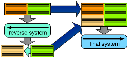
Figure 13.31: Creating synthetic parallel data from target-side monolingual data: (1) train a system in reverse order, (2) use it to translate target-side monolingual data into the source language, (3) combine the generated synthetic parallel data with the true parallel data in final system building.

• Train a reverse system that translates from the intended target language into the source language. We typically use the same neural machine translation setup for this as for our final system, just with source and target flipped. But we may use any system, even traditional phrase-based systems.

• Use the reverse system to translate target side monolingual data, creating a synthetic parallel corpus.

• Combine the generated synthetic parallel data with the true parallel data when building the final system.

There is an open question on how much synthetic parallel data should be used in relation to the amount of existing true parallel data. Typically, there are magnitudes more monolingual data available, but we also do not want to drown out the actual real data. Successful applications of this idea used equal amounts of synthetic and true data. We may also generate much more synthetic parallel data, but then ensure during training that we process equal amounts of each by over-sampling the true parallel data.

Adding a Language Model

The other idea is to train a language model as a separate component of the neural translation model. Gülçehre et al. (2015) first train the large language model as a recurrent neural network on all available data, including the target side of the parallel corpus. Then, they add this language model to the neural translation model. Since both language model and translation model predict output words, the natural point to connect the two models is joining them at that output prediction node in the network by concatenating their conditioning contexts.

We expand Equation 13.75 to add the hidden state of the neural language model $s^{\text{\sc lm}}_{i}$ to the hidden state of the neural translation model $s^{\text{\sc tm}}_{i}$, the source context $c_{i}$ and the previous English word $e_{i-1}$.

$$e_{i}=g(c_{i},s^{\text{\sc tm}}_{i},s^{\text{\sc lm}}_{i},e_{i-1})$$ (13.82)

When training the combined model, we leave the parameters of the large neural language model unchanged, and update only the parameters of the translation model and the combination layer. The concern is that otherwise the output side of the parallel corpus would overwrite the memory of the large monolingual corpus. In other words, the language model would overfit to the parallel training data and be less general.

One final question remains: How much weight should be given to the translation model and how much weight should be given to the language model? The above equation considers them in all instances the same way. But there may be output words for which the translation model is more relevant (e.g., the translation of content words with distinct meaning) and output words where the language model is more relevant (e.g., the introduction of relevant function words for fluency).

The balance of the translation model and the language model can be achieved with the type of gated units that we encountered in our discussion of the long short-term memory neural network architecture (Section 13.4.5). Such a gated unit may be predicted solely from the language model state $s^{\text{\sc lm}}_{i}$ and then used as a factor that is multiplied with that language model state before it is used in the prediction of Equation 13.82.

$$\text{gate}^{\text{\sc lm}}_{i} =f(s^{\text{\sc lm}}_{i})$$ (13.83)

$$\bar{s}^{\text{\sc lm}}_{i} =\text{gate}^{\text{\sc lm}}_{i}\times s^{\text{\sc lm}}_{i}$$

$$e_{i} =g(c_{i},s^{\text{\sc tm}}_{i},\bar{s}^{\text{\sc lm}}_{i},e_{i-1})$$

Round Trip Training

Looking at the backtranslation idea from a strict machine learning perspective, we can see two learning objectives. There is the objective to learn the transformations given by the parallel data, as done traditionally. Then, there is the goal to learn how to convert an output lamguage sentence into the input language, and then back into the output language with the objective to match the traditional sentence. A good machine translation model should be able to preserve the meaning of the output language sentence when mapped into the input language and back.

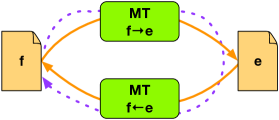
Figure 13.32: Round trip training: In addition to training two models f$\rightarrow$e and e$\rightarrow$f, as done traditionally on parallel data, we also optimize both models to convert a sentence $f$ into $e$ and then restore it back into $f$, using on monolingual data in $f$. We may add a corresponding round trip starting with $e$.

See Figure 13.32 for an illustration. There are two machine translation models. One that translates sentences in the language direction f$\rightarrow$e, the other in the opposite direction e$\rightarrow$f. These two systems may be trained with traditional means, using a parallel corpus. We can also round trip a sentence $f$ first through the f$\rightarrow$e and then back through e$\rightarrow$f

In this scenario, there are two objectives for model training.

• The translation e’ of the given monolingual sentence f should be a valid sentence in the language $e$, as measured with a language model $\text{\sc lm}_{e}(\text{\bf e'})$.

• The reconstruction of the translation e’ back into the original language $f$ should be easy, as measured with the translation model $\text{\sc mt}_{e\rightarrow f}(\text{\bf f}|\text{\bf e'})$

These two objectives can be used to update model parameters in both translation models $\text{\sc mt}_{f\rightarrow e}$ and $\text{\sc mt}_{e\rightarrow f}$.

Typical model update is driven by correct predictions of each word. In this round-trip scenario, the translation e’ has to be computed first, before we can do the usual training of model $\text{\sc mt}_{e\rightarrow f}$ with the given sentence pair (e’,f). To make better use of the training data, a n-best list of translations $\text{\bf e'}_{1},...,\text{\bf e'}_{n}$ is computed and model updates are computed for each of them.

We can also update the model $\text{\sc mt}_{f\rightarrow e}$ with monolingual data in language $f$ by scaling updates by the language model cost $\text{\sc lm}_{e}(\text{\bf e'}_{i})$ and the forward translation cost $\text{\sc mt}_{f\rightarrow e}(\text{\bf e'}_{i}|\text{\bf f})$ for each of the translations $\text{\bf e'}_{i}$ in the n-best list.

To use monolingual data in language $e$, training is done in the reverse round trip direction. For details of this idea, refer to Xia et al. (2016).

Further Readings

Sennrich et al. (2016c) back-translate the monolingual data into the input language and use the obtained synthetic parallel corpus as additional training data. Xia et al. (2016) use monolingual data in a dual learning setup. Machine translation engines are trained in both directions, and in addition to regular model training from parallel data, monolingual data is translated in a round trip (e to f to e) and evaluated with a language model for language f and reconstruction match back to e as cost function to drive gradient descent updates to the model.

Deep Models

Learning the lessons from other research fields such as vision or speech recognition, recent work in machine translation has also looked at deeper models. Simply put, this involves adding more intermediate layers into the baseline architecture.

The core components of neural machine translation are the encoder that takes input words and converts them into a sequence of contextualized representations and the decoder that generates a output sequence of words. Both are recurrent neural networks.

Recall that we already discussed how to build deeper recurrent neural networks for language modelling (refer back to Section 13.4.7). We now extend these ideas to the recurrent neural networks in the encoder and the decoder.

What all these recurrent neural networks have in common is that they process an input sequence into an output sequence, and at each time step $t$ information from a new input $x_{t}$ is combined with the hidden state from the previous time step $h_{t-1}$ to predict a new hidden state $h_{t}$. From that hidden state additional predictions may be made (output words $y_{t}$ in the case of the decoder, the next word in the sequence in the case of language models), or the hidden state is used otherwise (via the attention mechanism in case of the encoder).

Decoder

See Figure 13.33 for part of the decoder in neural machine translation, using a particular deeper architecture. We see that instead of a single hidden state $h_{t}$ for a given time step $t$, we now have a sequence of hidden states $h_{t,1}$, $h_{t,2}$, …, $h_{t,I}$ for a given time step $t$.

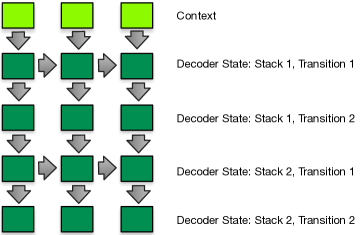
Figure 13.33: Deep Decoder: Instead of a single recurrent neural network (RNN) layer for the decoder state, in a deep model, it consists of several layers. The illustrations shows a combination of a deep transition and stacked RNNs. It omits the word prediction, word selection and output word embedding steps which are identical to the original architecture, shown in Figure 13.20.

There are various options how the hidden states may be connected. Previously, in Section 13.4.7 we presented two ideas. (1) In stacked recurrent neural networks where a hidden state $h_{t,i}$ is conditioned on the hidden state from a previous layer $h_{t,i-1}$ and the hidden state at the same depth from a previous time step $h_{t-1,i}$. (2) In deep transition recurrent neural networks, the first hidden state $h_{t,1}$ is conditioned on the last hidden state from the previous time step $h_{t-1,I}$ and the input, while the other hidden layers $h_{t,I}$ ($i>1$) are just conditioned on the previous previous layer $h_{t,i-1}$.

Figure 13.33 combines these two ideas. some layers are both stacked (conditioned on the previous time step $h_{t-1,I}$ and previous layer $h_{t,i-1}$), while others are deep transitions (conditioned only on the previous layer $h_{t,i-1}$.

Mathematically, we can break this out into the stacked layers $h_{t,i}$:

$$h_{t,1} =f_{1}(x_{t},h_{t-1,1})$$ (13.84)

$$h_{t,i} =f_{i}(h_{t,i-1},h_{t-1,i}) i>1$$ for

and the deep transition layers $v_{i,i,j}$.

$$v_{t,i,1} =g_{i,1}(\text{in}_{t,i},h_{t-1,i}) \text{in}_{t,i}\;\text{is either $x_{t}$ or $h_{t,i-1}$}$$ (13.85)

$$v_{t,i,j} =g_{i,j}(v_{t,i,j-1}) j>1$$ for

$$h_{t,i} =v_{t,i,J}$$

The function $f_{i}(h_{t,i-1},h_{t-1,i})$ is computed as a sequence of function calls $g_{i,j}$. Each of the functions $g_{i,j}$ may be implemented as feed-forward neural network layer (matrix multiplication plus activation function), long-short term memory cell (LSTM), or gated recurrent unit (GRU). On either case, each function $g_{i,j}$ has its own set of trainable model parameters.

Encoder

Deep recurrent neural networks for the encoder may draw in the same ideas as the decoder, with one addition: in the baseline neural translation model, we used bidirectional recurrent neural networks to condition on both left and right context. We want to do the same for any deep version of the encoder.

Figure 13.34 shows one idea how this could be done, called alternating recurrent neural network. It looks basically like a stacked recurrent neural network, with one twist: the hidden states at each layer $h_{t,i}$ are alternately conditioned on the hidden state from the previous time step $h_{t-1,i}$ or the next time step $h_{t+1,i}$.

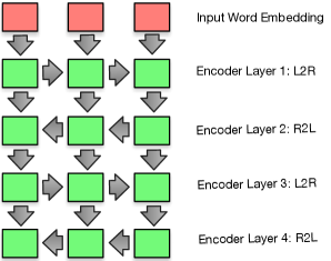
Figure 13.34: Deep alternating encoder: combination of the idea of a bidirectional recurrent neural network previously proposed for neural machine translation (recall Figure 13.19) and the stacked recurrent neural network (recall Figure 13.19). This architecture may be further extended with the idea of deep transitions, as shown for the decoder (previous Figure 13.33).

Mathematically, we formulate this as even numbered hidden states $h_{t,2i}$ being conditioned on the left context $h_{t-1,2i}$ and odd numbered hidden states $h_{t,2i+1}$ conditioned on the right context $h_{t+1,2i}$.

$$h_{t,1} =f(x_{t},h_{t-1,1})$$ (13.86)

$$h_{t,2i} =f(h_{t,2i-1},h_{t-1,2i})$$

$$h_{t,2i+1} =f(h_{t,2i},h_{t+1,2i+1})$$

As before in the encoder, we can extend this idea by having deep transitions.

Note that deep models are typically augmented with direct connections from the input to the output. In the case of the encoder, this may mean a direct connection from the embedding to the final encoder layer, or connections at each layer that pass the input directly to the output. Such residual connections help with training. In early stages, the deep architecture can be skipped. Only when a basic functioning model has been acquired, the deep architecture can be exploited to enrich it. We typically see the benefits of residual connections in early training stages (faster initial reduction of model perplexity), and less so as improvement in the final converged model.

Further Readings

Recent work has shown good results with 4 stacks and 2 deep transitions each for encoder and decoder, as well as alternating networks for the encoder (Miceli Barone et al., 2017). There are a large number of variations (including the use of skip connections, the choice of LSTM vs. GRU, number of layers of any type) that still need to be explored empirical for various data conditions.

Guided Alignment Training

The attention mechanism in neural machine translation models is motivated by the need to align output words to input words. Figure 13.35 shows an example of attention weights given to English input words for each German output word during the translation of a sentence.

Figure 13.35: Alignment vs. Attention: In this example, alignment points from traditional word alignment methods are shown as squares, and attention states as shaded boxes depending on the alignment value (shown as percentage). They generally match up well, but note for instance that the prediction of the output auxiliary verb sind pays attention to the entire verb group have been strained.

The attention values typically match up pretty well with word alignment used in traditional statistical machine translation, obtained with tools such as GIZA++ or fast-align which implement variants of the IBM Models.

There are several good uses for word alignments beyond their intrinsic value of improving the quality of translations. For instance in the next section, we will look at using the attention mechanism to explicitly track coverage of the input. We may also want to override preferences of the neural machine translation model with pre-specified translations of certain terminology or expressions such as numbers, dates, or measurements that are better handled by rule-based components; this requires to know when the neural model is about to translate a specific source word. But also the end user may be interested in alignment information, such as translators using machine translation in a computer aided translation tool may want to check where an output word originates from.

Hence, instead of trusting the attention mechanism to implicitly acquire the role as word alignmer, we may enforce this role. The idea is to provide not just the parallel corpus as training data, but also pre-computed word alignments using traditional means. Such additional information may even benefit training of models to converge faster or overcome data sparsity under low resource conditions.

A straightforward way to add such given word alignment to the training process is to not change the model at all, but to just modify the training objective. Typically, the goal of training neural machine translation models is to generate the correct output words. We can add to this goal to also match the given word alignment.

Formally, we assume to have access to an alignment matrix $A$ that specifies alignment points $A_{ij}$ input words $j$ and output words $i$ in a way that $\sum_{j}A_{ij}=1$, i.e., each output word’s alignment scores add up to 1. The model estimates attention scores $\alpha_{ij}$ that also add up to 1 for each output word: $\sum_{j}\alpha_{ij}=1$ (recall Equation 13.79). The mismatch between given alignment scores $A_{ij}$ and computed attention scores $\alpha_{ij}$ can be measured in several ways, such as cross entropy

$$\text{cost}_{\text{\sc ce}}=-\frac{1}{I}\sum_{i=1}^{I}\sum_{j=1}^{J}A_{ij}\;\text{log}\;\alpha_{ij}$$ (13.87)

or mean squared error

$$\text{cost}_{\text{\sc mse}}=-\frac{1}{I}\sum_{i=1}^{I}\sum_{j=1}^{J}(A_{ij}-\alpha_{ij})^{2}$$ (13.88)

This cost is added to the training objective and may be weighted.

Further Readings

Chen et al. (2016b); Liu et al. (2016) add supervised word alignment information (obtained with traditional statistical word alignment methods) to training. They augment the objective function to also optimize matching of the attention mechanism to the given alignments.

Modeling Coverage

One impressive aspect of neural machine translation models is how well they are able to translate the entire input sentence, even when a lot of reordering is involved. But this as aspect is not perfect, occasionally the model translates some input words multiple times, and sometimes it misses to translate them.

Figure 13.36: Example for over-generation and under-generation: the input tokens around Social Housing are attended too much, leading to hallucinated output words (das Unternehmen, English: the company), while the end of the sentence a fresh start is not attended and untranslated.

See Figure 13.36 for an example. The translation has two flaws related to mis-allocation of attention. The beginning of the phrase “Social Housing" alliance receives too much attention, resulting in a faulty translation with hallucinated words: das Unternehmen der Gesellschaft für soziale Bildung, or the company of the society for social education. At the end of the input sentence, the phrase a fresh start does not receive any attention and is hence untranslated in the output.

Hence, an obvious idea is to more strictly model coverage. Given the attention model, a reasonable way to define coverage is by adding up the attention states. In a complete sentence translation, we roughly expect that each input word receives a similar amount of attention. If some input words never receive attention or too much attention that signals a problem with the translation.

Enforcing Coverage during Inference

We may restrict the enforcing of proper coverage to the decoder. When considering multiple hypothesis in beam search, then we should discourage the ones that pay too much attention to some input words. And, once hypotheses are completed, we can penalize those that paid only little attention to some of the input. There are various ways to come up with scoring functions for over-generation and under-generation.

$$\text{coverage}(j) =\sum_{i}\sum_{k}\alpha_{i,k}$$ (13.89)

over-generation $$=\text{max}\Big{(}0,\sum_{j}\text{coverage}(j)-1\Big{)}$$

under-generation $$=\text{min}\Big{(}1,\sum_{j}\text{coverage}(j)\Big{)}$$

The use of multiple scoring functions in the decoder is common practice in traditional statistical machine translation. For now, it is not in neural machine translation. A challenge is to give proper weight to the different scoring functions. If there are only two or three weights, these can be optimized with grid search over possible values. For more weights, we may borrow methods such as MERT or MIRA from statistical machine translation.

Coverage Models

The vector that accumulates coverage of input words may be directly used to inform the attention model. Previously, the attention given to a specific input word $j$ was conditioned on the previous state of the decoder $s_{i-1}$ and the representation of the input word $h_{j}$. Now, we also add as conditioning context the accumulated attention given to the word (compare to Equation 13.78).

$$a(s_{i-1},h_{j})=W^{a}s_{i-1}+U^{a}h_{j}+V^{a}\text{coverage}(j)+b^{a}$$ (13.90)

Coverage tracking may also integrated into the training objective. Taking a page from the guided alignment training (recall the previous Section 13.6.5), we augment the training objective function with a coverage penalty with some weight $\lambda$.

$$\log\sum_{i}P(y_{i}|x)+\lambda\sum_{j}(1-\text{coverage}(j))^{2}$$ (13.91)

Note that in general, it is problematic to add such additional functions to the learning objective, since it does distract from the main goal of producing good translations.

Fertility

So far, we described coverage as the need to cover all input words roughly evenly. However, even the earliest statistical machine translation models considered the fertility of words, i.e., the number of output words that are generated from each input word. Consider the English do not construction: most other language do not require an equivalent of do when negating a verb. Meanwhile, other words are translated into multiple output words. For instance, the German natürlich may be translated as of course, thus generating 2 output words.

We may augment models of coverage by adding a fertility components that predicts the number of output words for each input words. Here one example for a model that predicts the fertility $\Phi_{j}$ for each input word, and uses it to normalize the coverage statistics.

$$\Phi_{j} =N\sigma(W_{j}h_{j})$$ (13.92)

$$\text{coverage}(j) =\frac{1}{\Phi_{j}}\sum_{i}\sum_{k}\alpha_{i,k}$$

Fertility $\Phi_{j}$ is predicted with a neural network layer that is conditioned on the input word representation $h_{j}$ and uses a sigmoid activation function (thus resulting in values from 0 to 1), which is scaled to a pre-defined maximum fertility of $N$.

Feature Engineering versus Machine Learning

The work on modeling coverage in neural machine translation models is a nice example to contrast between the engineering approach and the belief in generic machine learning techniques. From an engineering perspective, a good way to improve a system is to analyze its performance, find weak points and consider changes to overcome them. Here, we notice over-generation and under-generation with respect to the input, and add components to the model to overcome this problem. On the other hand, proper coverage is one of the features of a good translation that machine learning should be able to get from the training data. If it is not able to do that, it may need deeper models, more robust estimation techniques, ways to fight over-fitting or under-fitting, or other adjustments to give it just the right amount of power needed for the problem.

It is hard to carry out the analysis needed to make generic machine learning adjustments, given the complexity of a task like machine translation. Still, the argument for deep learning is that it does not require feature engineering, such as adding coverage models. It remains to be seen how neural machine translation evolves over the next years, and if it moves more into a engineering or machine learning direction.

Further Readings

To better model coverage, Tu et al. (2016b) add coverage states for each input word by either (a) summing up attention values, scaled by a fertility value predicted from the input word in context, or (b) learning a coverage update function as a feed-forward neural network layer. This coverage state is added as additional conditioning context for the prediction of the attention state. Feng et al. (2016) condition the prediction of the attention state also on the previous context state and also introduce a coverage state (initialized with the sum of input source embeddings) that aims to subtract covered words at each step. Similarly, Meng et al. (2016) separate hidden states that keep track of source coverage and hidden states that keep track of produced output. Cohn et al. (2016) add a number of biases to model coverage, fertility, and alignment inspired by traditional statistical machine translation models. They condition the prediction of the attention state on absolute word positions, the attention state of the previous output word in a limited window, and coverage (added attention state values) over a limited window. They also add a fertility model and add coverage in the training objective.

Adaptation

Text may differ by style, topic, degree of formality, and so on. A common problem in the practical development of machine translation systems is that most of the available training data is different from the data relevant to a chosen use case. For instance, if your goal is to translate chat room dialogs, you will realize that there is very little translated chat room data available. There are massive quantities of official publications from international organizations, random translations crawled from the web, and maybe somewhat relevant movie subtitle translations.

This problem is generally framed as a problem of domain adaptation. In the simplest form, you have one set of data relevant to your use case — the in-domain data — and another set that is less relevant — the out-of-domain data.

In traditional statistical machine translation, a vast number of methods for domain adaptation have been proposed. Models may be interpolated, we may back-off from in-domain to out-of-domain models, we may over-sample in-domain data during training or sub-sample out-of-domain data, etc.

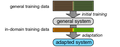
Figure 13.37: Online training of neural machine translation models allows a straightforward domain adaptation method: Having a general domain translation system trained on general-purpose data, a handful of additional training epochs on in-domain data allows for a domain-adapted system.

For neural machine translation, a fairly straightforward method is currently the most popular (see Figure 13.37). This method divides training up into two stages. First, we train the model on all available data until convergence. Then, we run a few more iterations of training on the in-domain data only and stop training when performance on the in-domain validate set peaks. This way, the final model benefits from all the training data, but is still specialized to the in-domain data.

Practical experience with this method shows that the second in-domain training stage may converge very quickly. The amount if in-domain data is typically relatively small, and only a handful of training epochs are needed.

Another, less commonly used method draws on the idea of ensemble decoding (Section 13.6.1). If we train separate models on different sets of data, we may combine their predictions, just as we did for ensemble decoding. In this case, we do want to choose weights for each model, although how to choose these weights is not a trivial task. If there is just an in-domain and out-of-domain model, however, this may be simply done by line search over possible values.

Let us now look at a few special cases that arise in practical use.

Subsample in-domain data from large collections

A common problem is that the amount of available in-domain data is very small, so just training on this data, even in a secondary adaptation stage, risks overfitting — very good performance on the seen data but poor performance on everything else.

Large random collections of parallel text often contain data that closely matches the in-domain data. So, we may want to extract this in-domain data from the large collections of mainly out-of-domain data. The general idea behind a variety of methods is to build two detectors: one in-domain detector trained on in-domain data, and one out-of-domain detector trained on out-of-domain data. We then score each sentence pair in the out-of-domain data with both detectors and select sentence pairs that are preferred (or judged relatively relevant) by the in-domain detector.

The classic detectors are language models trained on the source and target side of the in-domain and out-of-domain data, resulting in a total of 4 language models: the source side in-domain model $\text{LM}^{\text{in}}_{f}$, the target side in-domain model $\text{LM}^{\text{in}}_{e}$, the source side out-of-domain model $\text{LM}^{\text{out}}_{f}$, and the target side out-of-domain model $\text{LM}^{\text{out}}_{e}$. Any given sentence pair from the out-of-domain data is then scored based on these models:

$$\text{relevance}_{e,f}=\Big{(}\text{LM}^{\text{in}}_{e}(e)-\text{LM}^{\text{out}}_{e}(e)\Big{)}+\Big{(}\text{LM}^{\text{in}}_{f}(f)-\text{LM}^{\text{out}}_{f}(f)\Big{)}$$ (13.93)

We may use traditional n-gram language models or neural recurrent language models. Some work suggests to replace open class words (nouns, verbs, adjectives, adverbs) with part-of-speech tags or word clusters. More sophisticated models not only consider domain-relevance but noisiness of the training data (e.g., misaligned or mistranslated data). We may even use in-domain and out-of-domain neural translation models to score sentence pairs instead of source and target side sentences in isolation.

The subsampled data may be used in several ways. We may only train on this data to build our domain-specific system. Or, we use it in a secondary adaptation stage as outlined above.

Only monolingual in-domain data

What if we have no parallel data in the domain of our use case? Two main ideas have been explored. Firstly, we may still use the monolingual data, may it be in the source or target language or both, for subsampling parallel data from a large pile of general data, as outline above.

Another idea is to use existing parallel data to train an out-of-domain model, then back-translate out-of-domain data (recall Section 13.6.3) to generate a synthetic in-domain corpus, and then use this data to adapt the initial model. In traditional statistical machine translation, much adaptation success has been achieved with just interpolating the language model, and this idea is the neural translation equivalent to that.

Multiple domains

Sometimes, we have multiple collections of data that are clearly identified by domain — typically categories such as information technology, medical, law, etc. We can use the techniques described above to build specialized translation models for each of these domains.

For a given test sentence, we then select the appropriate model. If we do not know the domain of the test sentence, we first have to build a classifier that allows us to automatically make this determination. The classifier may be based on the methods for domain detectors described above. Given the decision of the classifier, we then select the most appropriate model.

But we do not have to commit to a single domain. The classifier may instead provide a distribution of relevance of the specific domain models (say, 50% domain A, 30% domain B, 20% domain C) which are then used as weights in an ensemble of domain-specific models.

The domain classification may done based on a whole document instead of each individual sentence, which brings in more context to make a more robust decision.

As a final remark, it is hard to give conclusive advice on how to handle adaptation challenges, since it is such a broad topic. The style of the text may be more relevant than its content. Data may differ narrowly (e.g., official publications from the United Nations vs. official announcements from the European Union) or dramatically (e.g., chat room dialogs vs. published laws). The amounts of in-domain and out-of-domain data differs. The data may be cleanly separated by domain or just come in a massive disorganized pile. Some of the data may be of higher translation quality than other, which may be polluted by noise such as mistranslations, misalignments, or even generated by some other machine translation system.

Further Readings

There is often a domain mismatch between the bulk (or even all) of the training data for a translation and its test data during deployment. There is rich literature in traditional statistical machine translation on this topic. A common approach for neural models is to first train on all available training data, and then run a few iterations on in-domain data only (Luong and Manning, 2015), as already pioneered in neural language model adaption (Ter-Sarkisov et al., 2015). Servan et al. (2016) demonstrate the effectiveness of this adaptation method with small in-domain sets consisting of as little as 500 sentence pairs.

Chu et al. (2017) argue that given small amount of in-domain data leads to overfitting and suggest to mix in-domain and out-of-domain data during adaption. Freitag and Al-Onaizan (2016) identify the same problem and suggest to use an ensemble of baseline models and adapted models to avoid overfitting. Peris et al. (2017) consider alternative training methods for the adaptation phase but do not find consistently better results than the traditional gradient descent training. Inspired by domain adaptation work in statistical machine translation on sub-sampling and sentence weighting, Chen et al. (2017) build an in-domain vs. out-of-domain classifier for sentence pairs in the training data, and then use its prediction score to reduce the learning rate for sentence pairs that are out of domain.

Farajian et al. (2017) show that traditional statistical machine translation outperforms neural machine translation when training general-purpose machine translation systems on a collection data, and then tested on niche domains. The adaptation technique allows neural machine translation to catch up.

A multi-domain model may be trained and informed at run-time about the domain of the input sentence. Kobus et al. (2016) apply an idea initially proposed by Sennrich et al. (2016a) - to augment input sentences for register with a politeness feature token - to the domain adaptation problem. They add a domain token to each training and test sentence. Chen et al. (2016b) report better results over the token approach to adapt to topics by encoding the given topic membership of each sentence as an additional input vector to the conditioning context of word prediction layer.

Adding Linguistic Annotation

One of the big debates in machine translation research is the question if the key to progress is to develop better, relatively generic, machine learning methods that implicitly learn the important features of language, or to use linguistic insight to augment data and models.

Recent work in statistical machine translation has demonstrated the benefits of linguistically motivated models. The best statistical machine translation systems in major evaluation campaigns for language pairs such as Chinese–English and German–English are syntax-based. While they translate sentences, they also build up the syntactic structure of the output sentence. There have been serious efforts to move towards deeper semantics in machine translation.

The turn towards neural machine translation was at first hard swing back towards better machine learning while ignoring much linguistic insights. Neural machine translation views translation as a generic sequence to sequence task, which just happens to involve sequences of words in different languages. Methods such as byte pair encoding or character-based translation models even put the value of the concept of a word as a basic unit into doubt.

However, recently there have been also attempts to add linguistic annotation into neural translation models, and steps towards more linguistically motivated models. We will take a look at successful efforts to integrate (1) linguistic annotation to the input sentence, (2) linguistic annotation to the output sentence, and (3) build linguistically structured models.

Linguistic annotation of the input

One of the great benefits of neural networks is their ability to cope with rich context. In the neural machine translation models we presented, each word prediction is conditioned on the entire input sentence and all previously generated output words. Even if, as it is typically the case, a specific input sequence and partially generated output sequence has never been observed before during training, the neural model is able to generalize the training data and draw from relevant knowledge. In traditional statistical models, this required carefully chosen independence assumptions and back-off schemes.

So, adding more information to the conditioning context in neural translation models can be accommodated rather straightforwardly. First, what information would be like to add? The typical linguistic treasure chest contains part-of-speech tags, lemmas, morphological properties of words, syntactic phrase structure, syntactic dependencies, and maybe even some semantic annotation.

All of these can be formatted as annotations to individual input words. Sometimes, this requires a bit more work, such as syntactic and semantic annotation that spans multiple words. See Figure 13.38 for an example. To just walk through the linguistic annotation of the word girl in the sentence:

Words	the	girl	watched	attentively	the	beautiful	fireflies
Part of speech	det	nn	adv	vfin	det	jj	nns
Lemma	the	girl	watch	attentive	the	beautiful	firefly
Morphology	-	sing.	past	-	-	plural
Noun phrase	begin	cont	other	other	begin	cont	cont
Verb phrase	other	other	begin	cont	cont	cont	cont
Synt. dependency	girl	watched	-	watched	fireflies	fireflies	watched
Depend. relation	det	subj	-	adv	det	adj	obj
Semantic role	-	actor	-	manner	-	mod	patient
Semantic type	-	human	view	-	-	-	animate

Figure 13.38: Linguistic annotation of a sentence, formatted as word-level factored representation

• Part of speech is nn, a noun.

• Lemma is girl, the same as the surface form. The lemma differs for watched / watch.

• Morphology is singular.

• The word is the continuation (cont) of the noun phrase that started with the.

• The word is not part of a verb phrase (other).

• Its syntactic head is watched.

• The dependency relationship to the head is subject (subj).

• Its semantic role is actor.

• There are many schemes of semantic types. For instance girl could be classified as human.

Note how phrasal annotations are handled. The first noun phrase is the girl. It is common to use an annotation scheme that tags individual words in a phrasal annation as begin and continuation (or intermediate), while labelling words outside such phrases as other.

How do we encode the word-level factored representation? Recall that words are initially represented as 1-hot vectors. We can encode each factor in the factored representation as a 1-hot vector. The concatenation of these vectors is then used as input to the word embedding. Note that mathematically this means, that each factor of the representation is mapped to a embedding vector, and the final word embedding is the sum of the factor embeddings.

Since the input to the neural machine translation system is still a sequence of word embeddings, we do not have to change anything in the architecture of the neural machine translation model. We just provide richer input representations and hope that the model is able to learn how to take advantage of it.

Coming back to the debate about linguistics versus machine learning. All the linguistic annotation proposed here can arguable be learned automatically as part of the word embeddings (or contextualized word embeddings in the hidden encoder states). This may or may not be true. But it does provide additional knowledge that comes from the tools that produce the annotation and that is particularly relevant if there is not enough training data to automatically induce it. Also, why make the job harder for the machine learning algorithm than needed? In other words, why force the machine learning to discover features that can be readily provided? Ultimately, these questions will be resolved empirically by demonstrating what actually works in specific data conditions.

Linguistic annotation of the output

What we have done for input words could be done also for output words. Instead of discussing the fine points about what adjustments need to made (e.g., separate softmax for each output factor), let us take a look at another annotation scheme for the output that has been successfully applied to neural machine translation.

Most syntax-based statistical machine translation models have focused on adding syntax to the output side. Traditional n-gram language models are good at promoting fluency among neighboring words, they are not powerful enough to ensure overall grammaticality of each output sentence. By designing models that also produce and evaluate the syntactic parse structure for each output sentence, syntax-based models give the means to promote grammatically correct output.

The word-level annotation of phrase structure syntax suggested in Figure 13.38 is rather crude. The nature of language is recursive, and annotating nested phrases cannot be easily handled with a begin/cont/other scheme. Instead, typically tree structures are used to represent syntax.

Sentence	the girl watched attentively the beautiful fireflies
Syntax tree	[.s [.np [.det the ] [.nn girl ] ] [.vp [.vfin watched ] [.advp [.adv attentively ] ] [.np [.det the ] [.jj beautiful ] [.nns fireflies ] ] ] ]
Linearized	(s (np (det the ) (nn girl ) ) (vp (vfin watched ) (advp (adv attentively ) ) (np (det the ) (jj beautiful ) (nns fireflies ) ) ) )

Figure 13.39: Linearization of phrase structure grammar tree into a sequence of words — e.g., girl, watched — and tags — e.g., (s, (np, )

See Figure 13.39 for an example. It shows the phrase structure syntactic parse tree for our example sentence The girl watched attentively the beautiful fireflies. Generating a tree structures is generally a quite different process than generating a sequence. It is typically built recursively bottom-up with algorithms such as chart parsing.

However, we can linearize the parse tree into a sequence of words and structural tokens that indicate the beginning — e.g., “(np" — and end — closing parenthesis “)" — of syntactic phrases. So, forcing syntactic parse tree annotations into our sequence-to-sequence neural machine translation model may be done by encoding the parse structure with additional output tokens. To be perfectly clear, the idea is to produce as the output of the neural translation system not just a sequence of words, but a sequence of a mix of output words and special tokens.

The hope is that forcing the neural machine translation model to produce syntactic structure (even in a linearized form) encourages it to produce syntactically well-formed output. There is some evidence to support this hope, despite the simplicity of the approach.

Linguistically structured models

The field of syntactic parsing has not been left untouched by the recent wave of neural networks. The previous section suggests that syntactic parsing may be done as simply as framing it as a sequence to sequence with additional output tokens.

However, the best-performing syntactic parsers use model structures that take the recursive nature of language to heart. They are either inspired by convolutional networks and build parse trees bottom-up, or are neural versions of left-to-right push-down automata that maintain a stack of opened phrases that any new word may extend or close, or be pushed down the stack to start a new phrase.

There is some early work on integrating syntactic parsing and machine translation into a unified framework but no consensus on best practices has emerged yet. At the time of writing, this is clearly still a challenge for future work.

Further Readings

Wu et al. (2012) propose to use factored representations of words (using lemma, stem, and part of speech), with each factor encoded in a one-hot vector, in the input to a recurrent neural network language model. Sennrich and Haddow (2016) use such representations in the input and output of neural machine translation models, demonstrating better translation quality.

Multiple Language Pairs

There are more than two languages in the world. And we also have training data for many language pairs, sometimes it is highly overlapping (e.g., European Parliament proceedings in 24 languages), sometimes it is unique (e.g. Canadian Hansards in French and English). For some language pairs, a lot of training data is available (e.g., French–English). But for most language pairs, there is only very little, including commercially interesting language pairs such as Chinese–German or Japanese–Spanish.

There is a long history of moving beyond specific languages and encode meaning language-independent, sometimes called interlingua. In machine translation, the idea is to map the input language first into an interlingua, and then map the interlingua into the output language. In such a system, we have to build just one mapping step into and one step out of the interlingua for each language. Then we can translate between it and all the other languages for which we have done the same.

Researchers in deep learning often do not hesitate to claim that intermediate states in neural translation models encode semantics or meaning. So, can we train a neural machine translation system that accepts text in any language as input and translates it into any other language?

Multiple Input Languages

Let us say, we have two parallel corpora, one for German–English, and one for French–English. We can train a neural machine translation model on both corpora at the same time by simply concatenating them. The input vocabulary contains both German and French words. Any input sentence will be quickly recognized as being either German or French, due to the sentence context, disambiguating words such as du (you in German, of in French).

The combined model trained on both data sets has one advantage over two separate models. It is exposed to both English sides of the parallel corpora and hence can learn a better language model. There may be also be general benefits to having diversity in the data, leading to more robust models.

Multiple Output Languages

We can do the same trick for the output language, by concatenating, say, a French–English and a French–Spanish corpus. But given a French input sentence during inference, how would the system know which output language to generate? A crude but effective way to signal this to the model is by adding a tag like [spanish] as first token of the input sentence.

[english] N’y a-t-il pas ici deux poids, deux mesures?
. $\Rightarrow$ Is this not a case of double standards?
[spanish] N’y a-t-il pas ici deux poids, deux mesures?
. $\Rightarrow$ No puede verse con toda claridad que estamos utilizando un doble rasero?

If we train a system on the three corpora mentioned (German–English, French–English, and French–Spanish) we can also use it translate a sentence from German to Spanish — without having ever presented a sentence pair as training data to the system.

[spanish] Messen wir hier nicht mit zweierlei Maß?
. $\Rightarrow$ No puede verse con toda claridad que estamos utilizando un doble rasero?

For this to work, there has to be some representation of the meaning of the input sentence that is not tied to the input language and the output language. Surprisingly, experiments show that this actually does work, somewhat. To achieve good quality, however, some parallel data in the desired language pair is needed, but much less than for a standalone model (Johnson et al., 2016).

Figure 13.40 summarizes this idea. A single neural machine translation is trained on various parallel corpora in turn, resulting in a system that may translate between any seen input and output language. It is likely that increasingly deeper models (recall Section 13.6.4) may better serve as multi-language translators, since their deeper layer compute more abstract representations of language.

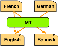
Figure 13.40: Multi-language machine translation system trained on one language pair at a time, rotating through many of them. After training on French–English, French–Spanish, and German–English, it is even able to translate from German to Spanish.

The idea of marking the output language with a token such as [spanish] has been explored more widely in the context of systems for a single language pair. Such tokens may represent the domain of the input sentence (Kobus et al., 2016), or the required level of politeness of the output sentence (Sennrich et al., 2016a).

Sharing Components

Instead of just throwing data at a generic neural machine translation model, we may want to more carefully consider which components may be shared among language-pair-specific models. The idea is to train one model per language pair, but some of the components are identical in these unique models.

• The encoder may be shared in models that have the same input language.

• The decoder may be shared in models that have the same output language.

• The attention mechanism may be shared in all models for all language pairs.

Sharing components means is that the same parameter values (weight matrices, etc.) are used in these separate models. Updates to them when training a model for one language pair then also changes them for in the model for the other language pairs. There is no need to mark the output language, since each model is trained for a specific language pair.

The idea of shared training of components can also be pushed further to exploit monolingual data. The encoder may be trained on monolingual input language data, but we will need to add a training objective (e.g., language model cross-entropy). Also, the decoder may be trained in isolation with monolingual language model data. However, since there are no context states available, these have to be blanked out, which may lead it to learn to ignore the input sentence and function only as a target side language model.

Further Readings

Johnson et al. (2016) explore how well a single canonical neural translation model is able to learn from multiple to multiple languages, by simultaneously training on on parallel corpora for several language pairs. They show small benefits for several input languages with the same output languages, mixed results for translating into multiple output languages (indicated by an additional input language token). The most interesting result is the ability for such a model to translate in language directions for which no parallel corpus is provided, thus demonstrating that some interlingual meaning representation is learned, although less well than using traditional pivot methods.

Firat et al. (2016) support multi-language input and output by training language-specific encoders and decoders and a shared attention mechanism.

Alternate Architectures

Most of neural network research has focused on the use of recurrent neural networks with attention. But this is by no means the only architecture for neural networks. Arguable, a disadvantage of using recurrent neural networks on the input side is that it requires a long sequential process that consumes each input word in one step. This also prohibits the ability to parallelize the processing of all words at once, thus limiting the use of the capabilities of GPUs.

There have been a few alternate suggestions for the architecture of neural machine translation models. We will briefly present some of them in this section. It remains to be seen, if they are a curiosity or conquer the field.

Convolutional Neural Networks

The first end-to-end neural machine translation model of the modern era (Kalchbrenner and Blunsom, 2013) was actually not based on recurrent neural networks, but based on convolutional neural networks. These had been shown to be very successful in image processing, thus looking for other applications was a natural next step.

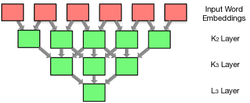
Figure 13.41: Encoding a sentence with a convolutional neural network. By always using two convolutional layers, the size of the convolutions differ (here $K_{2}$ and $K_{3}$). Decoding reverses this process.

See Figure 13.41 for an illustration of a convolutional network that encodes an input sentence. The basic building block of these networks is a convolution. It merges the representation of $i$ input words into a single representation by using a matrix $K_{i}$. Applying the convolution to every sequence of input words reduces the length of the sentence representation by $i-1$. Repeating this process leads to a sentence representation in a single vector.

The illustration shows an architecture with two convolutional $K_{i}$ layers, followed by a final $L_{i}$ layer that merges the sequence of phrasal representations into a single sentence representation. The size of the convolutional kernels $K_{i}$ and $L_{i}$ depends on the length of the sentences. The example shows a 6-word sentence and a sequence of $K_{2}$, $K_{3}$, and $L_{3}$ layers. For longer sentences, bigger kernels are needed.

The hierarchical process of building up a sentence representation bottom-up is well grounded in linguistic insight in the recursive nature of language. It is similar to chart parsing, except that we are not committing to a single hierarchical structure. On the other hand, we are asking an awful lot from the resulting sentence embedding to represents the meaning of an entire sentence of arbitrary length.

Generating the output sentence translation reverses the bottom-up process. One problem for the decoder is to decide the length of the output sentence. One option to address this problem is to add a model that predicts output length from input length. This then leads to the selection of the size of the reverse convolution matrices.

See Figure 13.42 for an illustration of a variation of this idea. The shown architecture always uses a $K_{2}$ and a $K_{3}$ convolutional layer, resulting in a sequence of phrasal representations, not a single sentence embedding. There is an explicit mapping step from phrasal representations of input words to phrasal representations of output words, called transfer layer.

The decoder of the model includes a recurrent neural network on the output side. Sneaking in a recurrent neural network here does undermine a bit the argument about better parallelization. However, the claim still holds true for encoding the input, and a sequential language model is just a too powerful tool to disregard.

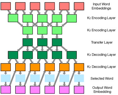
Figure 13.42: Refinement of the convolutional neural network model. Convolutions do not result in a single sentence embedding but a sequence. The encoder is also informed by a recurrent neural network (connections from output word embeddings to final decoding layer.

While the just-described convolutional neural machine translation model helped to set the scene for neural network approaches for machine translation, it could not be demonstrated to achieve competitive results compared to traditional approaches. The compression of the sentence representation into a single vector is especially a problem for long sentences. However, the model was used successfully in reranking candidate translations generated by traditional statistical machine translation systems.

Convolutional Neural Networks With Attention

Gehring et al. (2017) propose an architecture for neural networks that combines the ideas of convolutional neural networks and the attention mechanism. It is essentially the sequence-to-sequence attention that we described as the canonical neural machine translation approach, but with the recurrent neural networks replaced by convolutional layers.

We introduced convolutions in the previous section. The idea is to combine a short sequence of neighboring words into a single representation. To look at it in another way, a convolution encodes a word with its left and right context, in a limited window. Let us now describe in more detail what this means for the encoder and the decoder in the neural model.

Encoder

See Figure 13.43 for an illustration of the convolutional layers used in the encoder. For each input word, the state at each layer is informed by the corresponding state in the previous layer and its two neighbors. Note that these convolutional layers do not shorten the sequence, because we have a convolution centered around each word, using padding (vectors with zero values) for word positions that are out of bounds.

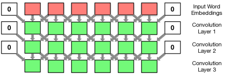
Figure 13.43: Encoder using stacked convolutional layers. Any number of layers may be used.

Mathematically, we start with the input word embeddings $Ex_{j}$ and progress through a sequence of layer encodings $h_{d,j}$ at different depth $d$ until a maximum depth $D$.

$$h_{0,j} =E\;x_{j}$$ (13.94)

$$h_{d,j} =f(h_{d-1,j-k},...,h_{d-1,j+k}) d>0 d\leq D$$ for ,

The function $f$ is a feed-forward layer, with a residual connection from the corresponding previous layer state $h_{d-1,j}$.

Note that even with a few convolutional layers, the final representation of a word $h_{D,j}$ may only be informed by partial sentence context — in contrast to the bi-directional recurrent neural networks in the canonical model. However, relevant context words in the input sentence that help with disambiguation may be outside this window.

On the other hand, there are significant computational advantages to this idea. All words at one depth can be processed in parallel, even combined into one massive tensor operation that can be efficiently parallelized on a GPU.

Decoder

The decoder in the canonical model also has at its core a recurrent neural network. Recall its state progression defined in Equation 13.75:

$$s_{i}=f(s_{i-1},\;Ey_{i-1},c_{i})$$ (13.95)

where $s_{i}$ is the encoder state, $Ey_{i-1}$ the embedding of the previous output word, and $c_{i}$ the input context.

The convolutional version of this does not have recurrent decoder states, i.e., the computation does not depend on the previous state $s_{i-1}$, but is conditioned on the sequence of the $\kappa$ most recent previous words.

$$s_{i}=f(Ey_{i-\kappa},...,Ey_{i-1},c_{i})$$ (13.96)

Furthermore, these decoder convolutions may be stacked, just as the encoder convolutional layers.

$$s_{1,i} =f(Ey_{i-\kappa},...,Ey_{i-1},c_{i})$$ (13.97)

$$s_{d,i} =f(s_{d-1,i-\kappa-1},...,s_{d-1,i},c_{i}) d>0 d\leq\hat{D}$$ for ,

See Figure 13.44 for an illustration of these equations. The main difference between the canonical neural machine translation model and this architecture is the conditioning of the states of the decoder. They are computed in a sequence of convolutional layers, and also always the input context.

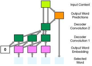
Figure 13.44: Decoder in convolutional neural network with attention. The decoder state is computed as a sequence of convolutional layers (here: 2) over the already predicted output words. Each convolutional state is also informed by the input context computed from the input sentence and attention.

Attention

The attention mechanism is essentially unchanged from the canonical neural translation model. Recall that is is based on an association $a(s_{i-1},h_{j})$ between the word representations computed by the encoder $h_{j}$ and the previous state of the decoder $s_{i-1}$ (refer back to Equation 13.78).

Since we still have such encoder and decoder states ($h_{D,j}$ and $s_{\hat{D},{i-1}}$), we use the same here. These association scores are normalized and used to compute a weighted sum of the input word embeddings (i.e., the encoder states $h_{D,j}$). A refinement is that the encoder state $h_{D,j}$ and the input word embedding $x_{j}$ is combined via addition when computing the context vector. This is the usual trick of using residual connections to assist training with deep neural networks.

Self-Attention

The critique of the use of recurrent neural networks is that they require a lengthy walk-through, word by word, of the entire input sentence, which is time-consuming and limits parallelization. The previous sections replaced the recurrent neural networks in our canonical model with convolutions. However, these have a limited context window to enrich representations of words. What we would like is some architectural component that allows us to use wide context and can be highly parallelized. What could that be?

In fact, we already encountered it: the attention mechanism. It considers associations between every input word and any output word, and uses it to build a vector representation of the entire input sequence. The idea behind self-attention is to extend this idea to the encoder. Instead of computing the association between an input and an output word, self-attention computes the association between any input word and any other input word. One way to view it is that this mechanism refines the representation of each input word by enriching it with context words that help to disambiguate it.

Computing Self-Attention

Vaswani et al. (2017) define self attention for a sequence of vectors $h_{j}$ (of size $|h|$), packed into a matrix $H$, as

$$\text{self-attention}(H)=\text{softmax}\Big{(}\frac{HH^{T}}{\sqrt{|h|}}\Big{)}H$$ (13.98)

Let us look at this equation in detail. The association between every word representation $h_{j}$ any other context word $h_{k}$ is done via the dot product between the packed matrix $H$ and its transpose $H^{T}$, resulting in a vector of raw association values $HH^{T}$. The values in this vector are first scaled by the size of the word representation vectors $|h|$, and then by the softmax, so that their values add up to 1. The resulting vector of normalized association values is then used to weigh the context words.

Another way to put Equation 13.98 without the matrix $H$ notation but using word representation vectors $h_{j}$:

$$a_{jk} =\frac{1}{|h|}h_{j}h_{k}^{T} \Big{(}\frac{HH^{T}}{\sqrt{|h|}}\Big{)}$$ raw association (13.99)

$$\alpha_{jk} =\frac{\text{exp}(a_{jk})}{\sum_{\kappa}\text{exp}(a_{j\kappa})}$$ normalized association (softmax)

$$\text{self-attention}(h_{j}) =\sum_{k}\alpha_{j\kappa}h_{k}$$ weighted sum

Self-Attention Layer

The self-attention step described above is only one step in the self-attention layer used to encode the input sentence. There are four more steps that follow it.

• We combine self-attention with residual connections that pass the word representation through directly

  $$\text{self-attention}(h_{j})+h_{j}$$ (13.100)

• Next up is a layer normalization step (described in Section 13.2.6).

  $$\hat{h}_{j}=\text{layer-normalization}(\text{self-attention}(h_{j})+h_{j})$$ (13.101)

• A standard feed-forward step with ReLU activation function is applied.

  $$\text{relu}(W\hat{h}_{j}+b)$$ (13.102)

• This is also augmented with residual connections and layer normalization.

  $$\text{layer-normalization}(\text{relu}(W\hat{h}_{j}+b)+\hat{h}_{j})$$ (13.103)

Taking a page from deep models, we now stack several such layers (say, $D=6$) on top of each other.

$$h_{0,j} =Ex_{j}$$ start with input word embedding (13.104)

$$h_{d,j} =\text{self-attention-layer}(h_{d-1,j}) d>0 d\leq D$$ for ,

The deep modeling is the reason behind the residual connections in the self-attention layer — such residual connections help with training since they allow a shortcut to the input which may be utilized in early stages of training, before it can take advantage of the more complex interdependencies that deep models enable. The layer normalization step is one standard training trick that also helps especially with deep models.

Attention in the Decoder

Self-attention is also used in the decoder, now between output words. The decoder also has more traditional attention. In total there are 3 sub layers.

• Self attention: Output words are initially encoded by word embeddings $s_{i}=Ey_{i}$. We perform exactly the same self-attention computation as described in Equation 13.98. However, the association of a word $s_{i}$ is limited to words $s_{k}$ with $k\leq i$, i.e., just the previously produced output words. Let us denote the result of this sub layer for output word $i$ as $\tilde{s_{i}}$

• Attention: The attention mechanism in this model follows very closely self-attention. The only difference is that, previously, we compute self attention between the hidden states $H$ and themselves. Now, we compute attention between the decoder states $\tilde{S}$ and the final encoder states $H$.

  $$\text{attention}(\tilde{S},H)=\text{softmax}\Big{(}\frac{\tilde{S}H^{T}}{\sqrt{|h|}}\Big{)}H$$ (13.105)

  Using the same more detailed exposition as above for self-attention:

  $$a_{ik} =\frac{1}{|h|}\tilde{s}_{i}h_{k}^{T} \Big{(}\frac{\tilde{S}H^{T}}{\sqrt{|h|}}\Big{)}$$ raw association (13.106)

  $$\alpha_{ik} =\frac{\text{exp}(a_{ik})}{\sum_{\kappa}\text{exp}(a_{i\kappa})}$$ normalized association (softmax)

  $$\text{attention}(\tilde{s}_{i}) =\sum_{k}\alpha_{j\kappa}h_{k}$$ weighted sum

  This attention computation is augmented by adding in residual connections, layer normalization, and an additional ReLU layer, just like the self-attention layer described above.

  It is worth noting that, the output of the attention computation is a weighted sum over input word representations $\sum_{k}\alpha_{j\kappa}h_{k}$. To this, we add the (self-attended) representation of the decoder state $\tilde{s}_{i}$ via a residual connection. This allows skipping over the deep layers, thus speeding up training.

• Feed-forward layer: This sub layer is identical to the encoder, i.e., $\text{relu}(W_{s}\hat{s}_{i}+b_{s})$

Each of the sub-layers is followed by the add-and-norm step of first using residual connections and then layer normalization (as noted in the description of the attention sub layer).

The entire model is shown in Figure 13.45,

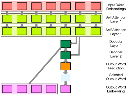
Figure 13.45: Attention-based machine translation model: the input is encoded with several layers of self-attention. The decoder computes attention-based representations of the input in several layers, initialized with the previous word embeddings.

Further Readings

Kalchbrenner and Blunsom (2013) build a comprehensive machine translation model by first encoding the source sentence with a convolutional neural network, and then generate the target sentence by reversing the process. A refinement of this was proposed by Gehring et al. (2017) who use multiple convolutional layers in the encoder and the decoder that do not reduce the length of the encoded sequence but incorporate wider context with each layer.

Vaswani et al. (2017) replace the recurrent neural networks used in attentional sequence-to-sequence models with multiple self-attention layers, both for the encoder as well as the decoder. There are a number of additional refinements of this model: so-called multi-head attention, encoding of sentence positions of words, etc.

Current Challenges

Neural machine translation has emerged as the most promising machine translation approach in recent years, showing superior performance on public benchmarks (Bojar et al., 2016) and rapid adoption in deployments by, e.g., Google (Wu et al., 2016), Systran (Crego et al., 2016), and WIPO (Junczys-Dowmunt et al., 2016). But there have also been reports of poor performance, such as the systems built under low-resource conditions in the DARPA LORELEI program.

Here, we examine a number of challenges to neural machine translation and give empirical results on how well the technology currently holds up, compared to traditional statistical machine translation. We show that, despite its recent successes, neural machine translation still has to overcome various challenges, most notably performance out-of-domain and under low resource conditions.

What a lot of the problems have in common is that the neural translation models do not show robust behavior when confronted with conditions that differ significantly from training conditions — may it be due to limited exposure to training data, unusual input in case of out-of-domain test sentences, or unlikely initial word choices in beam search. The solution to these problems may hence lie in a more general approach of training that steps outside optimizing single word predictions given perfectly matching prior sequences.

Another challenge that we do not examine empirically: neural machine translation systems are much less interpretable. The answer to the question of why the training data leads these systems to decide on specific word choices during decoding is buried in large matrices of real-numbered values. There is a clear need to develop better analytics for neural machine translation.

We use common toolkits for neural machine translation (Nematus) and traditional phrase-based statistical machine translation (Moses) with common data sets, drawn from WMT and OPUS. Unless noted otherwise, we use default settings, such as beam search and single model decoding. The training data is processed with byte-pair encoding (Sennrich et al., 2016c) into subwords to fit a 50,000 word vocabulary limit.

Our statistical machine translation systems are trained using Moses (Koehn et al., 2007). We build phrase-based systems using standard features that are commonly used in recent system submissions to WMT (Williams et al., 2016; Ding et al., 2016). While we consider here only phrase-based systems, we note that there are other statistical machine translation approaches such as hierarchical phrase-based models (Chiang, 2007) and syntax-based models (Galley et al., 2004, 2006) that have been shown to give superior performance for language pairs such as Chinese–English and German–English.

We carry out our experiments on English–Spanish and German–English. For these language pairs, large training data sets are available. We use datasets from the shared translation task organized alongside the Conference on Machine Translation (WMT). For the domain experiments, we use the OPUS corpus (Tiedemann, 2012).

Except for the domain experiments, we use the WMT test sets composed of news stories, which are characterized by a broad range of topic, formal language, relatively long sentences (about 30 words on average), and high standards for grammar, orthography, and style.

Domain Mismatch

A known challenge in translation is that in different domains, words have different translations and meaning is expressed in different styles. Hence, a crucial step in developing machine translation systems targeted at a specific use case is domain adaptation. We expect that methods for domain adaptation will be developed for neural machine translation. A currently popular approach is to train a general domain system, followed by training on in-domain data for a few epochs (Luong and Manning, 2015; Freitag and Al-Onaizan, 2016).

Often, large amounts of training data are only available out of domain, but we still seek to have robust performance. To test how well neural machine translation and statistical machine translation hold up, we trained five different systems using different corpora obtained from OPUS (Tiedemann, 2012). An additional system was trained on all the training data. Statistics about corpus sizes are shown in Table 13.3. Note that these domains are quite distant from each other, much more so than, say, Europarl, TED Talks, News Commentary, and Global Voices.

Corpus	Words	Sentences	W/S
Law (Acquis)	18,128,173	715,372	25.3
Medical (EMEA)	14,301,472	1,104,752	12.9
IT	3,041,677	337,817	9.0
Koran (Tanzil)	9,848,539	480,421	20.5
Subtitles	114,371,754	13,873,398	8.2

Table 13.3: Corpora used to train domain-specific systems, taken from the OPUS repository. IT corpora are GNOME, KDE, PHP, Ubuntu, and OpenOffice.

We trained both statistical machine translation and neural machine translation systems for all domains. All systems were trained for German-English, with tuning and test sets sub-sampled from the data (these were not used in training). A common byte-pair encoding is used for all training runs.

System $\downarrow$	Law	Medical	IT	Koran	Subtitles

Figure 13.46: Quality of systems (BLEU), when trained on one domain (rows) and tested on another domain (columns). Comparably, neural machine translation systems (left bars) show more degraded performance out of domain.

See Figure 13.46 for results. While the in-domain neural and statistical machine translation systems are similar (neural machine translation is better for IT and Subtitles, statistical machine translation is better for Law, Medical, and Koran), the out-of-domain performance for the neural machine translation systems is worse in almost all cases, sometimes dramatically so. For instance the Medical system leads to a BLEU score of 3.9 (neural machine translation) vs. 10.2 (statistical machine translation) on the Law test set.

Figure 13.47 displays an example. When translating the sentence Schaue um dich herum. (reference: Look around you.) from the Subtitles corpus, we see mostly non-sensical and completely unrelated output from the neural machine translation system. For instance, the translation from the IT system is Switches to paused.

Note that the output of the neural machine translation system is often quite fluent (e.g., Take heed of your own souls.) but completely unrelated to the input, while the statistical machine translation output betrays its difficulties with coping with the out-of-domain input by leaving some words untranslated (e.g., Schaue by dich around.). This is of particular concern when MT is used for information gisting — the user will be mislead by hallucinated content in the neural machine translation output.

Source	Schaue um dich herum.
Reference	Look around you.
All	NMT: Look around you.
	SMT: Look around you.
Law	NMT: Sughum gravecorn.
	SMT: In order to implement dich Schaue .
Medical	NMT: EMEA / MB / 049 / 01-EN-Final Work progamme for 2002
	SMT: Schaue by dich around .
IT	NMT: Switches to paused.
	SMT: To Schaue by itself . \t \t
Koran	NMT: Take heed of your own souls.
	SMT: And you see.
Subtitles	NMT: Look around you.
	SMT: Look around you .

Figure 13.47: Examples for the translation of a sentence from the Subtitles corpus, when translated with systems trained on different corpora. Performance out-of-domain is dramatically worse for neural machine translation.

Amount of Training Data

A well-known property of statistical systems is that increasing amounts of training data lead to better results. In statistical machine translation systems, we have previously observed that doubling the amount of training data gives a fixed increase in BLEU scores. This holds true for both parallel and monolingual data (Turchi et al., 2008; Irvine and Callison-Burch, 2013).

Figure 13.48: BLEU scores for English-Spanish systems trained on 0.4 million to 385.7 million words of parallel data. Quality for neural machine translation starts much lower, outperforms statistical machine translation at about 15 million words, and even beats a statistical machine translation system with a big 2 billion word in-domain language model under high-resource conditions.

How do the data needs of statistical machine translation and neural machine translation compare? Neural machine translation promises both to generalize better (exploiting word similarity in embeddings) and condition on larger context (entire input and all prior output words).

We built English-Spanish systems on WMT data, about 385.7 million English words paired with Spanish. To obtain a learning curve, we used $\frac{1}{1024}$, $\frac{1}{512}$, …, $\frac{1}{2}$, and all of the data. For statistical machine translation, the language model was trained on the Spanish part of each subset, respectively. In addition to a neural and statistical machine translation system trained on each subset, we also used all additionally provided monolingual data for a big language model in contrastive statistical machine translation systems.

Results are shown in Figure 13.48. Neural machine translation exhibits a much steeper learning curve, starting with abysmal results (BLEU score of 1.6 vs. 16.4 for $\frac{1}{1024}$ of the data), outperforming statistical machine translation 25.7 vs. 24.7 with $\frac{1}{16}$ of the data (24.1 million words), and even beating the statistical machine translation system with a big language model with the full data set (31.1 for neural machine translation, 28.4 for statistical machine translation, 30.4 for statistical with a big language model).

The contrast between the neural and statistical machine translation learning curves is quite striking. While neural machine translation is able to exploit increasing amounts of training data more effectively, it is unable to get off the ground with training corpus sizes of a few million words or less.

To illustrate this, see Figure 13.49. With $\frac{1}{1024}$ of the training data, the output is completely unrelated to the input, some key words are properly translated with $\frac{1}{512}$ and $\frac{1}{256}$ of the data (estrategia for strategy, elección or elecciones for election), and starting with $\frac{1}{64}$ the translations become respectable.

Ratio	Words	Source: A Republican strategy to counter the re-election of Obama
$\frac{1}{1024}$	0.4 million	Un órgano de coordinación para el anuncio de libre determinación
$\frac{1}{512}$	0.8 million	Lista de una estrategia para luchar contra la elección de hojas de Ohio
$\frac{1}{256}$	1.5 million	Explosión realiza una estrategia divisiva de luchar contra las elecciones de autor
$\frac{1}{128}$	3.0 million	Una estrategia republicana para la eliminación de la reelección de Obama
$\frac{1}{64}$	6.0 million	Estrategia siria para contrarrestar la reelección del Obama .
$\frac{1}{32}+$	12.0 million	Una estrategia republicana para contrarrestar la reelección de Obama

Figure 13.49: Translations of the first sentence of the test set using neural machine translation system trained on varying amounts of training data. Under low resource conditions, neural machine translation produces fluent output unrelated to the input.

Noisy Data

Statistical machine translation is fairly robust to noisy data. The quality of systems holds up fairly well, even if large parts of the training data are corrupted in various ways, such as misaligned sentences, content in wrong languages, badly translated sentences, etc. Statistical machine translation models are built on probability distributions estimated from many occurrences of words and phrases. Any unsystematic noise in the training only affects the tail end of the distribution.

Is this still the case for neural machine translation? Chen et al. (2016a) considered one kind of noise: misaligned sentence pairs in an experiments with a large English–French parallel corpus. They shuffle the target side of part of the training corpus, so that these sentence pairs are mis-aligned.

Table 13.4 shows the result. Statistical machine translation systems hold up fairly well. Even with 50% of the data perturbed, the quality only drops from 32.7 to 32.0 bleu points, about what is to be expected with half the valid training data. However, the neural machine translation system degrades severely, from 35.4 to 30.1 bleu points, a drop of 5.3 points, compared to the 0.7 point drop for statistical systems.

Ratio shuffled	0%	10%	20%	50%
SMT (bleu)	32.7	32.7 (–0.0)	32.6 (–0.1)	32.0 (–0.7)
NMT (bleu)	35.4	34.8 (–0.6)	32.1 (–3.3)	30.1 (–5.3)

Table 13.4: Impact of noise in the training data, with parts of the training corpus shuffled to contain mis-aligned sentence pairs. Neural machine translation degrades severely, while statistical machine translation holds up fairly well.

A possible explanation for this poor behavior of neural machine translation models is that its prediction has to find a good balance between language model and input context as the main driver. When training observes increasing ratios of training example, for which the input sentence is a meaningless distraction, it may generally learn to rely more on the output language model aspect, hence hallucinating fluent by inadequate output.

Word Alignment

The key contribution of the attention model in neural machine translation (Bahdanau et al., 2015) was the imposition of an alignment of the output words to the input words. This takes the shape of a probability distribution over the input words which is used to weigh them in a bag-of-words representation of the input sentence.

Arguably, this attention model does not functionally play the role of a word alignment between the source in the target, at least not in the same way as its analog in statistical machine translation. While in both cases, alignment is a latent variable that is used to obtain probability distributions over words or phrases, arguably the attention model has a broader role. For instance, when translating a verb, attention may also be paid to its subject and object since these may disambiguate it. To further complicate matters, the word representations are products of bidirectional gated recurrent neural networks that have the effect that each word representation is informed by the entire sentence context.

But there is a clear need for an alignment mechanism between source and target words. For instance, prior work used the alignments provided by the attention model to interpolate word translation decisions with traditional probabilistic dictionaries (Arthur et al., 2016), for the introduction of coverage and fertility models (Tu et al., 2016b), etc.

But is the attention model in fact the proper means? To examine this, we compare the soft alignment matrix (the sequence of attention vectors) with word alignments obtained by traditional word alignment methods. We use incremental fast-align (Dyer et al., 2013) to align the input and output of the neural machine system.

See Figure 13.50a for an illustration. We compare the word attention states (green boxes) with the word alignments obtained with fast align (blue outlines). For most words, these match up pretty well. Both attention states and fast-align alignment points are a bit fuzzy around the function words have-been/sind.

However, the attention model may settle on alignments that do not correspond with our intuition or alignment points obtained with fast-align. See Figure 13.50b for the reverse language direction, German–English. All the alignment points appear to be off by one position. We are not aware of any intuitive explanation for this divergent behavior — the translation quality is high for both systems.

(a) Desired Alignment	(b) Mismatched Alignment

Figure 13.50: Word alignment for English–German: comparing the attention model states (green boxes with probability in percent if over 10) with alignments obtained from fast-align (blue outlines).

We measure how well the soft alignment (attention model) of the neural machine translation system match the alignments of fast-align with two metrics:

• a match score that checks for each output if the aligned input word according to fast-align is indeed the input word that received the highest attention probability, and

• a probability mass score that sums up the probability mass given to each alignment point obtained from fast-align.

In these scores, we have to handle byte pair encoding and many-to-many alignments

In out experiment, we use the neural machine translation models provided by Edinburgh (Sennrich et al., 2016b). We run fast-align on the same parallel data sets to obtain alignment models and used them to align the input and output of the neural machine translation system. Table 13.5 shows alignment scores for the systems. The results suggest that, while drastic, the divergence for German–English is an outlier. We note, however, that we have seen such large a divergence also under different data conditions.

Language Pair	Match	Prob.
German–English	14.9%	16.0%
English–German	77.2%	63.2%
Czech–English	78.0%	63.3%
English–Czech	76.1%	59.7%
Russian–English	72.5%	65.0%
English–Russian	73.4%	64.1%

Table 13.5: Scores indicating overlap between attention probabilities and alignments obtained with fast-align.

Note that the attention model may produce better word alignments by guided alignment training (Chen et al., 2016b; Liu et al., 2016) where supervised word alignments (such as the ones produced by fast-align) are provided to model training.

Beam Search

Figure 13.51: Translation quality with varying beam sizes. For large beams, quality decreases, especially when not normalizing scores by sentence length.

The task of decoding is to find the full sentence translation with the highest probability. In statistical machine translation, this problem has been addressed with heuristic search techniques that explore a subset of the space of possible translation. A common feature of these search techniques is a beam size parameter that limits the number of partial translations maintained per input word.

There is typically a straightforward relationship between this beam size parameter and the model score of resulting translations and also their quality score (e.g., BLEU). While there are diminishing returns for increasing the beam parameter, typically improvements in these scores can be expected with larger beams.

Decoding in neural translation models can be set up in similar fashion. When predicting the next output word, we may not only commit to the highest scoring word prediction but also maintain the next best scoring words in a list of partial translations. We record with each partial translation the word translation probabilities (obtained from the softmax), extend each partial translation with subsequent word predictions and accumulate these scores. Since the number of partial translation explodes exponentially with each new output word, we prune them down to a beam of highest scoring partial translations.

As in traditional statistical machine translation decoding, increasing the beam size allows us to explore a larger set of the space of possible translation and hence find translations with better model scores.

However, as Figure 13.51 illustrates, increasing the beam size does not consistently improve translation quality. In fact, in almost all cases, worse translations are found beyond an optimal beam size setting (we are using again Edinburgh’s WMT 2016 systems). The optimal beam size varies from 4 (e.g., Czech–English) to around 30 (English–Romanian).

Normalizing sentence level model scores by length of the output alleviates the problem somewhat and also leads to better optimal quality in most cases (5 of the 8 language pairs investigated). Optimal beam sizes are in the range of 30–50 in almost all cases, but quality still drops with larger beams. The main cause of deteriorating quality are shorter translations under wider beams.

Further Readings

Other studies have looked at the comparable performance of neural and statistical machine translation systems. Bentivogli et al. (2016) considered different linguistic categories for English–German and Toral and Sánchez-Cartagena (2017) compared different broad aspects such as fluency and reordering for nine language directions.

Additional Topics

Especially early work on neural networks for machine translation was aimed at building neural components to be used in traditional statistical machine translation systems.

Translation Models

By including aligned source words in the conditioning context, Devlin et al. (2014) enrich a feed-forward neural network language model with source context Zhang et al. (2015) add a sentence embedding to the conditional context of this model, which are learned using a variant of convolutional neural networks and mapping them across languages. Meng et al. (2015) use a more complex convolutional neural network to encode the input sentence that uses gated layers and also incorporates information about the output context.

Reordering Models

Lexicalized reordering models struggle with sparse data problems when conditioned on rich context. Li et al. (2014) show that a neural reordering model can be conditioned on current and previous phrase pair (encoded with a recursive neural network auto-encoder) to make the same classification decisions for orientation type.

Pre-Ordering

Instead of handing reordering within the decoding process, we may pre-order the input sentence into output word order. de Gispert et al. (2015) use an input dependency tree to learn a model that swaps children nodes and implement it using a feed-forward neural network. Miceli Barone and Attardi (2015) formulate a top-down left-to-right walk through the dependency tree and make reordering decisions at any node. They model this process with a recurrent neural network that includes past decisions in the conditioning context.

N-Gram Translation Models

An alternative view of the phrase based translation model is to break up phrase translations into minimal translation units, and employing a n-gram model over these units to condition each minimal translation units on the previous ones. Schwenk et al. (2007) treat each minimal translation unit as an atomic symbol and train a neural language model over it. Alternatively, (Hu et al., 2014) represent the minimal translation units as bag of words, (Wu et al., 2014) break them even further into single input words, single output words, or single input-output word pairs, and Yu and Zhu (2015) use phrase embeddings leaned with an auto-encoder.

Author Index

Ahn, Sungjin 61

Akhanov, Egor 88

Al-Onaizan, Yaser 75, 89

Amos, David 11

Arthur, Philip 61, 95

Attardi, Giuseppe 99

Attik, Mohammed 45

Auli, Michael 83, 88, 99

Ba, Jimmy 23

Bahdanau, Dzmitry 6, 57, 94

Baltescu, Paul 45

Barrault, Loïc 75

Bengio, Yoshua 6, 23, 33, 45, 57, 61, 63, 81, 94

Bentivogli, Luisa 98

Bertoldi, Nicola 75, 89

Birch, Alexandra 62, 65, 68, 75, 81, 89, 96

Bisazza, Arianna 98

Blunsom, Phil 6, 45, 82, 88

Bojar, Ondřej 88, 89

Bougares, Fethi 45, 63, 75

Brunelle, Patrice 88

Byrne, Bill 5, 99

Callison-Burch, Chris 89, 91

Cao, Yuan 88

Casacuberta, Francisco 5, 75

Castaño, M. Asunción 5

Cebrián, Luis 75

Cettolo, Mauro 98

Chahuneau, Victor 95

Chatterjee, Rajen 88

Chen, Boxing 75, 94

Chen, Wenhu 69, 75, 96

Chen, Zhenbiao 5

Chen, Zhifeng 80, 81, 88

Cherry, Colin 75, 94

Chiang, David 45, 89

Cho, Kyunghyun 6, 45, 57, 61, 63, 81, 94

Chu, Chenhui 75

Cohn, Trevor 72

Constantin, Alexandra 89

Coquard, Aurelien 88

Corrado, Greg 80, 81, 88

Costa-jussa, Marta Ruiz 99

Courville, Aaron 23

Cowan, Brooke 89

Crego, Josep 75, 81

Crego, Josep Maria 75, 88

Cristianini, Nello 91

Dabre, Raj 75

Dauphin, Yann N. 83, 88

De Bie, Tijl 91

de Gispert, Adrià 5, 99

Dean, Jeffrey 80, 81, 88

Dechelotte, Daniel 45

DeNeefe, Steve 89

Deng, Yongchao 88

Devlin, Jacob 6, 98

Ding, Shuoyang 89

Dixon, Paul 45

Dong, Daxiang 99

Ducharme, Réjean 33, 45

Duchi, John 23

Duh, Kevin 89

Dwojak, Tomasz 88

Dyer, Chris 72, 95

Dyer, Christopher J. 89

Enoue, Satoshi 88

Farajian, M. Amin 75

Federico, Marcello 75, 89, 98

Federmann, Christian 88

Feng, Shi 72

Finch, Andrew 45, 69, 96

Firat, Orhan 6, 45, 63, 81

Fonollosa, Jose A. R. 99

Forcada, Mikel L 5

Fossum, Victoria 45

Foster, George 75, 94

Freiberg, Ben 45

Freitag, Markus 75, 89

Galley, Michel 89

Gao, Jianfeng 99

Gao, Qin 88, 99

Gauvain, Jean-Luc 45

Gehring, Jonas 83, 88

Geiss, Chiyo 88

Gemici, Mevlana 11

Goldberg, Yoav 23

Gomez, Aidan N. 86, 88

Goodfellow, Ian 23

Goto, Isao 45

Gouws, Stephan 88

Graehl, Jonathan 89

Graham, Yvette 88

Grangier, David 83, 88

Gu, Jiatao 62

Gulcehre, Caglar 61

Haddow, Barry 62, 65, 68, 75, 79, 81, 88, 89, 96

Haffari, Gholamreza 72

Hao, Jie 98

Hauptmann, A.G. 5

Hazan, Elad 23

He, Di 65

He, Wei 99

Helcl, Jindřich 68

Herbst, Evan 89

Hinton, G. E. 23

Hinton, Geoffrey 23

Hoang, Cong Duy Vu 72

Hoang, Hieu 45, 88, 89

Hopkins, Mark 89

Hori, Chiori 79

Hu, Xiaoguang 99

Hu, Yuening 99

Huang, Fei 94

Huang, Zhongqiang 6, 98

Huck, Matthias 88, 89

Hughes, Macduff 80, 81, 88

Hung, Chia-Chun 11

Iglesias, Gonzalo 5, 99

Irvine, Ann 91

Ittycheriah, Abe 62

Izuha, Tatsuya 5, 99

Jain, A. N. 5

Jauvin, Christian 33, 45

Jean, Sébastien 6, 61

Jiang, Wenbin 98

Jimeno Yepes, Antonio 88

Johanson, Joshua 88

Johnson, Melvin 80, 81, 88

Jones, Llion 86, 88

Junczys-Dowmunt, Marcin 88

Kaiser, Lukasz 86, 88

Kalchbrenner, Nal 6, 82, 88

Kanouchi, Shin 5

Kashioka, Hideki 79

Kato, Yoshikiyo 88

Kayser, Michael 44, 45

Kazawa, Hideto 88

Khadivi, Shahram 69, 75, 96

Khalsa, Ardas 88

Khayrallah, Huda 89

Khiari, Raoum 88

Kim, Jungi 88

Kingma, Diederik P. 23

Kiros, J. R. 23

Klein, Guillaume 88

Klingner, Jeff 88

Knight, Kevin 89

Ko, Byeongil 88

Kobus, Catherine 75, 81, 88

Koehn, Philipp 88, 89

Komachi, Mamoru 5

Krikun, Maxim 80, 81, 88

Krizhevsky, Alex 23

Kudo, Taku 88

Kuhn, Roland 94

Kurian, George 88

Kurohashi, Sadao 75

Lamar, Thomas 6, 98

Larkin, Samuel 75

Le, Quoc 61

Le, Quoc V. 80, 81, 88

Le, Quoc V. V 6, 57

Lei Ba, J. 23

Li, Hang 57, 62, 72, 95, 98

Li, Mu 72

Li, Peng 5, 99

Li, Victor O.K. 62

Lillicrap, Timothy P. 11

Lin, Huei-Chi 45, 63

Liu, Lemao 69, 96

Liu, Qun 72, 98

Liu, Shujie 72

Liu, Tie-Yan 65

Liu, Ting 99

Liu, Xiaobing 88

Liu, Xiaohua 57, 72, 95

Liu, Yang 5, 57, 72, 95, 99

Logacheva, Varvara 88

Lorieux, Jean 88

Lu, Bao-Liang 45

Lu, Shixiang 5

Lu, Xugang 79

Lu, Zhengdong 57, 62, 72, 95, 98

Luong, Minh-Thang 75, 89

Luong, Thang 44, 45, 57, 61

Ma, Wei-Ying 65

Macherey, Klaus 88

Macherey, Wolfgang 88

Makhoul, John 6, 98

Manning, Christopher 75, 89

Manning, Christopher D. 44, 45, 57

Marcu, Daniel 89

Martins, Leidiana 88

Matsuda, Shigeki 79

Matusov, Evgeny 69, 75, 96

McNair, A. E. 5

Memisevic, Roland 6, 61

Meng, Fandong 72, 98

Mi, Haitao 62

Miceli Barone, Antonio Valerio 68, 99

Mikolov, Tomas 23, 35, 45

Mohamed, Shakir 11

Monz, Christof 88

Moran, Christine 89

Nadejde, Maria 89

Nakamura, Satoshi 61, 95

Nallapati, Ramesh 61

Ñeco, Ramón P 5

Negri, Matteo 75, 88

Neubig, Graham 61, 95

Neveol, Aurelie 88

Neves, Mariana 88

Ney, Hermann 45

Nguyen, Dang-Chuan 88

Norouzi, Mohammad 88

Oparin, Ilya 45

Parmar, Niki 86, 88

Pascanu, Razvan 23

Patil, Nishant 88

Peris, Álvaro 75

Peter, Jan-Thorsten 69, 75, 96

Pham, Hieu 57

Polosukhin, Illia 86, 88

Popel, Martin 88

Post, Matt 88, 89

Priori, Alexandra 88

Qin, Tao 65

Rebollo, Anabel 88

Rezende, Danilo Jimenez 11

Riccardi, Thomas 88

Riesa, Jason 88

Rousseau, Anthony 45

Rubino, Raphael 88

Rudnick, Alex 88

Saito, H. 5

Salakhutdinov, Ruslan 23

Sánchez-Cartagena, Víctor M. 98

Santoro, Adam 11

Scarton, Carolina 88

Schl
"uter, Ralf 45

Schuster, Mike 80, 81, 88

Schwartz, Richard 6, 98

Schwenk, Holger 5, 45, 63, 75, 99

Segal, Natalia 88

Senellart, Jean 75, 81, 88

Sennrich, Rico 62, 65, 68, 75, 79, 81, 89, 96

Servan, Christophe 75, 88

Shah, Apurva 88

Shang, Lifeng 57

Shazeer, Noam 86, 88

Shen, Wade 89

Singer, Yoram 23

Smith, Jason 88

Smith, Noah A. 95

Specia, Lucia 88

Srivastava, Nitish 23

Stevens, Keith 88

Sudoh, Katsuhito 5

Sumita, Eiichiro 45, 69, 96

Sumita, Eiichro 45

Sun, Maosong 5, 99

Sundermeyer, Martin 45

Sutskever, Ilya 6, 23, 57, 61

Tebelskis, J. 5

Ter-Sarkisov, Alex 75

Thayer, Ignacio 89

Thorat, Nikhil 80, 81

Tiedemann, Jörg 89

Tiquet, Cyril 88

Toral, Antonio 98

Tu, Zhaopeng 57, 72, 95

Turchi, Marco 75, 88, 91

Uszkoreit, Jakob 86, 88

Utiyama, Masao 45, 69, 96

van Merrienboer, Bart 6, 57

Vaswani, Ashish 45, 86, 88

Verspoor, Karin 88

Vidal, Enrique 5

Viégas, Fernanda B. 80, 81

Vincent, Pascal 33, 45

Vinyals, Oriol 6, 57, 61, 88

Vymolova, Ekaterina 72

Waibel, A. 5

Wang, Bo 88

Wang, Haifeng 99

Wang, Liwei 65

Wang, Mingxuan 98

Wang, Rui 45

Wang, Wei 88, 89

Wang, Zhiguo 62

Wattenberg, Martin 80, 81

Wayne, Greg 11

Williams, Philip 89

Wu, Haiyang 99

Wu, Hua 99

Wu, Yonghui 80, 81, 88

Wu, Youzheng 79

Xia, Yingce 65

Xu, Bo 5

Xu, Kelvin 45, 63

Yamamoto, Hitoshi 79

Yang, Jin 88

Yang, Kathy 88

Yang, Nan 72

Yao, Kaisheng 72

Yarats, Denis 83, 88

Yih, Wen-tau 35

Young, Cliff 88

Yu, Dianhai 99

Yu, Heng 99

Yu, Nenghai 65

Zampieri, Marcos 88

Zaremba, Wojciech 61

Zbib, Rabih 6, 98

Zeiler, Matthew D. 23

Zens, Richard 89

Zhang, Dakun 5, 88, 98, 99

Zhang, Jiajun 98

Zhao, Hai 45

Zhao, Yinggong 45

Zhou, Bowen 61

Zhou, Jing 88

Zhou, Ming 72

Zhu, Kenny Q. 72

Zhu, Xuan 99

Zoldan, Peter 88

Zweig, Geoffrey 35

Index

• 1-hot vector §13.4.1
• activation function §13.2.3
• acyclical directed graph §13.3.1
• Adagrad §13.2.6
• Adam §13.2.6
• adaptation §13.6.7
• alignment §13.5.2
  • evaluation §13.8.4
• alternating recurrent neural network §13.6.4
• amount of training data §13.8.2
• attention §13.5.2
  • self-attention §13.7.3
• back translation §13.6.3
• back-propagation §13.2.5
  • through time §13.4.4
• backward pass §13.3.2
• batch training §13.2.6
• beam §13.5.4
• beam search §13.5.4
  • evaluation §13.8.5
• bidirectional recurrent neural network §13.5.2
• byte pair encoding §13.6.2
• cell (LSTM) §13.4.5
• chain rule §13.3.2
• checkpoint ensemble §13.6.1
• clipping footnote 6
• computation graph §13.3.1
  • dynamic §13.4.4
• computation node §13.3.1
• convolutional neural network §13.7.1
• coverage §13.6.6
• data
  • in-domain §13.6.7
  • monolingual §13.6.3
  • noisy §13.8.3
  • out-of-domain §13.6.7
  • size §13.8.2
  • synthetic 2nd item
• decoder §13.5.1
• decoding
  • forced §13.6.1
• deep learning §13.2.3
  • framworks §13.3.3
• deep model §13.4.7, §13.6.4
• deep transition §13.4.7
• deeply stacked §13.4.7
• direct connection §13.4.1
• distributional lexical semantics §13.4.2
• domain adaptation §13.6.7
• drop-out §13.2.6
• dual learning §13.6.3
• dynamic computation graph §13.4.4
• DyNet §13.3.3
• embedding
  • sentence §13.5.1
  • word §13.4.1
• encoder §13.5.1
• encoder-decoder §13.5.1
• ensemble §13.6.1
  • checkpoint §13.6.1
  • multi-run §13.6.1
• epoch §13.2.5
• error term §13.2.5
• exploding gradient footnote 6
• feed-forward neural network §13.4.1
• fertility §13.6.6
• forced decoding §13.6.1
• forget gate 2nd item
• forward pass §13.3.2
• framework §13.3.3
• garden path problem §13.5.4
• gate §13.4.5
  • forget 2nd item
  • index 1st item
  • output 3rd item
• gated recurrent unit §13.4.6
• GPU §13.2.6
• gradient
  • clipping footnote 6
  • exploding footnote 6
• gradient descent §13.2.5
• graphics processing unit §13.2.6
• GRU §13.4.6
• guided alignment training §13.6.5
• hidden layer §13.2.2
• highway connection §13.4.1
• history §13.1
• Hogwild §13.2.6
• hyperbolic tangent §13.2.3
• hypothesis §13.5.4
• in-domain data §13.6.7
• inference §13.2.4
• initialization §13.2.6
• input gate 1st item
• language model §13.4
  • feed-forward §13.4.1
  • recurrent §13.4.4
• layer normalization §13.2.6
• learning
  • online §13.2.6
• learning rate §13.2.5
• linear model §13.2.1
• linearization of parse tree §13.6.8
• linguistic annotation §13.6.8
• logistic function §13.2.3
• long short-term memory §13.4.5
• LSTM §13.4.5
• mask §13.5.3
• match score (alignment) 1st item
• matrix §13.2.6
• mini batch §13.2.6, §13.5.3
• model
  • deep §13.4.7, §13.6.4
• momentum term §13.2.6
• monolingual data §13.6.3
• multi-run ensemble §13.6.1
• multiple language pairs §13.6.9
• neural language model §13.4
  • feed-forward §13.4.1
  • recurrent §13.4.4
• neural network
  • alternating recurrent §13.6.4
  • bidirectional recurrent §13.5.2
  • convolutional §13.7.1
  • feed-forward §13.4.1
  • recurrent §13.4.4
• neural Turing machines §13.2.4
• noisy data §13.8.3
• non-linear §13.2.3
• one hot vector §13.4.1
• online learning §13.2.6
• out-of-domain data §13.6.7
• output gate 3rd item
• over-fitting §13.2.6
• probability mass score (alignment) 2nd item
• pyTorch §13.3.3
• rectified linear unit §13.2.3
• recurrent neural language model §13.4.4
• recurrent neural network §13.4.4
  • alternating §13.6.4
  • bidirectional §13.5.2
• ReLU §13.2.3
• reranking §13.6.1
• residual connection §13.4.1, §13.6.4
• right-to-left §13.6.1
• RNN §13.4.4
• round trip §13.6.3
• self-attention §13.7.3
• semantics §13.4.2
• sentence embedding §13.5.1
• size of training data §13.8.2
• skip connection §13.4.1
• softmax §13.4.1
• stacked §13.4.7
• stochastic gradient descent §13.2.6
• subword units §13.6.2
• synthetic parallel corpus 2nd item
• tangent §13.2.3
• tensor §13.2.6
• Tensorflow §13.3.3
• Theano §13.3.3
• Torch §13.3.3
• tuning §13.2.1
• unfolding §13.4.4
• unrolling §13.5.3
• validation set §13.2.6
• vector §13.2.6
• vocabulary §13.6.2
• word alignment §13.8.4
• word embedding §13.4.1

References

- Arthur et al. (2016) Philip Arthur, Graham Neubig, and Satoshi Nakamura. 2016. Incorporating discrete translation lexicons into neural machine translation. In Proceedings of the 2016 Conference on Empirical Methods in Natural Language Processing. Association for Computational Linguistics, Austin, Texas, pages 1557–1567. https://aclweb.org/anthology/D16-1162.
- Bahdanau et al. (2015) Dzmitry Bahdanau, Kyunghyun Cho, and Yoshua Bengio. 2015. Neural machine translation by jointly learning to align and translate. In ICLR. http://arxiv.org/pdf/1409.0473v6.pdf.
- Baltescu and Blunsom (2015) Paul Baltescu and Phil Blunsom. 2015. Pragmatic neural language modelling in machine translation. In Proceedings of the 2015 Conference of the North American Chapter of the Association for Computational Linguistics: Human Language Technologies. Association for Computational Linguistics, Denver, Colorado, pages 820–829. http://www.aclweb.org/anthology/N15-1083.
- Baltescu et al. (2014) Paul Baltescu, Phil Blunsom, and Hieu Hoang. 2014. Oxlm: A neural language modelling framework for machine translation. The Prague Bulletin of Mathematical Linguistics 102:81–92. http://ufal.mff.cuni.cz/pbml/102/art-baltescu-blunsom-hoang.pdf.
- Bengio et al. (2003) Yoshua Bengio, Réjean Ducharme, Pascal Vincent, and Christian Jauvin. 2003. A neural probabilistic language model. Journal of Machine Learning Research (3):1137–1155.
- Bentivogli et al. (2016) Luisa Bentivogli, Arianna Bisazza, Mauro Cettolo, and Marcello Federico. 2016. Neural versus phrase-based machine translation quality: a case study. In Proceedings of the 2016 Conference on Empirical Methods in Natural Language Processing. Association for Computational Linguistics, Austin, Texas, pages 257–267. https://aclweb.org/anthology/D16-1025.
- Bojar et al. (2016) Ondřej Bojar, Rajen Chatterjee, Christian Federmann, Yvette Graham, Barry Haddow, Matthias Huck, Antonio Jimeno Yepes, Philipp Koehn, Varvara Logacheva, Christof Monz, Matteo Negri, Aurelie Neveol, Mariana Neves, Martin Popel, Matt Post, Raphael Rubino, Carolina Scarton, Lucia Specia, Marco Turchi, Karin Verspoor, and Marcos Zampieri. 2016. Findings of the 2016 conference on machine translation. In Proceedings of the First Conference on Machine Translation. Association for Computational Linguistics, Berlin, Germany, pages 131–198. http://www.aclweb.org/anthology/W/W16/W16-2301.
- Castaño et al. (1997) M. Asunción Castaño, Francisco Casacuberta, and Enrique Vidal. 1997. Machine translation using neural networks and finite-state models. pages 160–167. http://www.mt-archive.info/TMI-1997-Castano.pdf.
- Chen et al. (2017) Boxing Chen, Colin Cherry, George Foster, and Samuel Larkin. 2017. Cost weighting for neural machine translation domain adaptation. In Proceedings of the First Workshop on Neural Machine Translation. Association for Computational Linguistics, Vancouver, pages 40–46. http://www.aclweb.org/anthology/W17-3205.
- Chen et al. (2016a) Boxing Chen, Roland Kuhn, George Foster, Colin Cherry, and Fei Huang. 2016a. Bilingual methods for adaptive training data selection for machine translation. In Annual Meeting of the Association for Machine Translation in the Americas (AMTA). http://www-labs.iro.umontreal.ca/ foster/papers/bicnn-data-sel-amta16.pdf.
- Chen et al. (2016b) Wenhu Chen, Evgeny Matusov, Shahram Khadivi, and Jan-Thorsten Peter. 2016b. Guided alignment training for topic-aware neural machine translation. CoRR abs/1607.01628. http://arxiv.org/abs/1607.01628.
- Chiang (2007) David Chiang. 2007. Hierarchical phrase-based translation. Computational Linguistics 33(2). http://www.aclweb.org/anthology-new/J/J07/J07-2003.pdf.
- Cho et al. (2014) Kyunghyun Cho, Bart van Merrienboer, Dzmitry Bahdanau, and Yoshua Bengio. 2014. On the properties of neural machine translation: Encoder–decoder approaches. In Proceedings of SSST-8, Eighth Workshop on Syntax, Semantics and Structure in Statistical Translation. Association for Computational Linguistics, Doha, Qatar, pages 103–111. http://www.aclweb.org/anthology/W14-4012.
- Chu et al. (2017) Chenhui Chu, Raj Dabre, and Sadao Kurohashi. 2017. An empirical comparison of domain adaptation methods for neural machine translation. In Proceedings of the 55th Annual Meeting of the Association for Computational Linguistics (Volume 2: Short Papers). Association for Computational Linguistics, Vancouver, Canada, pages 385–391. http://aclweb.org/anthology/P17-2061.
- Cohn et al. (2016) Trevor Cohn, Cong Duy Vu Hoang, Ekaterina Vymolova, Kaisheng Yao, Chris Dyer, and Gholamreza Haffari. 2016. Incorporating structural alignment biases into an attentional neural translation model. In Proceedings of the 2016 Conference of the North American Chapter of the Association for Computational Linguistics: Human Language Technologies. Association for Computational Linguistics, San Diego, California, pages 876–885. http://www.aclweb.org/anthology/N16-1102.
- Crego et al. (2016) Josep Maria Crego, Jungi Kim, Guillaume Klein, Anabel Rebollo, Kathy Yang, Jean Senellart, Egor Akhanov, Patrice Brunelle, Aurelien Coquard, Yongchao Deng, Satoshi Enoue, Chiyo Geiss, Joshua Johanson, Ardas Khalsa, Raoum Khiari, Byeongil Ko, Catherine Kobus, Jean Lorieux, Leidiana Martins, Dang-Chuan Nguyen, Alexandra Priori, Thomas Riccardi, Natalia Segal, Christophe Servan, Cyril Tiquet, Bo Wang, Jin Yang, Dakun Zhang, Jing Zhou, and Peter Zoldan. 2016. Systran’s pure neural machine translation systems. CoRR abs/1610.05540. http://arxiv.org/abs/1610.05540.
- de Gispert et al. (2015) Adrià de Gispert, Gonzalo Iglesias, and Bill Byrne. 2015. Fast and accurate preordering for smt using neural networks. In Proceedings of the 2015 Conference of the North American Chapter of the Association for Computational Linguistics: Human Language Technologies. Association for Computational Linguistics, Denver, Colorado, pages 1012–1017. http://www.aclweb.org/anthology/N15-1105.
- Devlin et al. (2014) Jacob Devlin, Rabih Zbib, Zhongqiang Huang, Thomas Lamar, Richard Schwartz, and John Makhoul. 2014. Fast and robust neural network joint models for statistical machine translation. In Proceedings of the 52nd Annual Meeting of the Association for Computational Linguistics (Volume 1: Long Papers). Association for Computational Linguistics, Baltimore, Maryland, pages 1370–1380. http://www.aclweb.org/anthology/P14-1129.
- Ding et al. (2016) Shuoyang Ding, Kevin Duh, Huda Khayrallah, Philipp Koehn, and Matt Post. 2016. The jhu machine translation systems for wmt 2016. In Proceedings of the First Conference on Machine Translation. Association for Computational Linguistics, Berlin, Germany, pages 272–280. http://www.aclweb.org/anthology/W/W16/W16-2310.
- Duchi et al. (2011) John Duchi, Elad Hazan, and Yoram Singer. 2011. Adaptive subgradient methods for online learning and stochastic optimization. Journal of Machine Learning Research 12(Jul):2121–2159.
- Dyer et al. (2013) Chris Dyer, Victor Chahuneau, and Noah A. Smith. 2013. A simple, fast, and effective reparameterization of ibm model 2. In Proceedings of the 2013 Conference of the North American Chapter of the Association for Computational Linguistics: Human Language Technologies. Association for Computational Linguistics, Atlanta, Georgia, pages 644–648. http://www.aclweb.org/anthology/N13-1073.
- Farajian et al. (2017) M. Amin Farajian, Marco Turchi, Matteo Negri, Nicola Bertoldi, and Marcello Federico. 2017. Neural vs. phrase-based machine translation in a multi-domain scenario. In Proceedings of the 15th Conference of the European Chapter of the Association for Computational Linguistics: Volume 2, Short Papers. Association for Computational Linguistics, Valencia, Spain, pages 280–284. http://www.aclweb.org/anthology/E17-2045.
- Feng et al. (2016) Shi Feng, Shujie Liu, Nan Yang, Mu Li, Ming Zhou, and Kenny Q. Zhu. 2016. Improving attention modeling with implicit distortion and fertility for machine translation. In Proceedings of COLING 2016, the 26th International Conference on Computational Linguistics: Technical Papers. The COLING 2016 Organizing Committee, Osaka, Japan, pages 3082–3092. http://aclweb.org/anthology/C16-1290.
- Finch et al. (2012) Andrew Finch, Paul Dixon, and Eiichiro Sumita. 2012. Rescoring a phrase-based machine transliteration system with recurrent neural network language models. In Proceedings of the 4th Named Entity Workshop (NEWS) 2012. Association for Computational Linguistics, Jeju, Korea, pages 47–51. http://www.aclweb.org/anthology/W12-4406.
- Firat et al. (2016) Orhan Firat, Kyunghyun Cho, and Yoshua Bengio. 2016. Multi-way, multilingual neural machine translation with a shared attention mechanism. In Proceedings of the 2016 Conference of the North American Chapter of the Association for Computational Linguistics: Human Language Technologies. Association for Computational Linguistics, San Diego, California, pages 866–875. http://www.aclweb.org/anthology/N16-1101.
- Forcada and Ñeco (1997) Mikel L Forcada and Ramón P Ñeco. 1997. Recursive hetero-associative memories for translation. In Biological and Artificial Computation: From Neuroscience to Technology, Springer, pages 453–462.
- Freitag and Al-Onaizan (2016) Markus Freitag and Yaser Al-Onaizan. 2016. Fast domain adaptation for neural machine translation. Technical report. https://arxiv.org/pdf/1612.06897v1.pdf.
- Galley et al. (2006) Michel Galley, Jonathan Graehl, Kevin Knight, Daniel Marcu, Steve DeNeefe, Wei Wang, and Ignacio Thayer. 2006. Scalable inference and training of context-rich syntactic translation models. In Proceedings of the 21st International Conference on Computational Linguistics and 44th Annual Meeting of the Association for Computational Linguistics. Association for Computational Linguistics, Sydney, Australia, pages 961–968. http://www.aclweb.org/anthology/P/P06/P06-1121.
- Galley et al. (2004) Michel Galley, Mark Hopkins, Kevin Knight, and Daniel Marcu. 2004. What’s in a translation rule? In Proceedings of the Joint Conference on Human Language Technologies and the Annual Meeting of the North American Chapter of the Association of Computational Linguistics (HLT-NAACL). http://www.aclweb.org/anthology/N04-1035.pdf.
- Gehring et al. (2017) Jonas Gehring, Michael Auli, David Grangier, Denis Yarats, and Yann N. Dauphin. 2017. Convolutional sequence to sequence learning. CoRR abs/1705.03122. http://arxiv.org/abs/1705.03122.
- Gemici et al. (2017) Mevlana Gemici, Chia-Chun Hung, Adam Santoro, Greg Wayne, Shakir Mohamed, Danilo Jimenez Rezende, David Amos, and Timothy P. Lillicrap. 2017. Generative temporal models with memory. CoRR abs/1702.04649. http://arxiv.org/abs/1702.04649.
- Goldberg (2017) Yoav Goldberg. 2017. Neural Network Methods for Natural Language Processing, volume 37 of Synthesis Lectures on Human Language Technologies. Morgan & Claypool, San Rafael, CA. https://doi.org/10.2200/S00762ED1V01Y201703HLT037.
- Goodfellow et al. (2016) Ian Goodfellow, Yoshua Bengio, and Aaron Courville. 2016. Deep Learning. MIT Press. http://www.deeplearningbook.org.
- Gu et al. (2016) Jiatao Gu, Zhengdong Lu, Hang Li, and Victor O.K. Li. 2016. Incorporating copying mechanism in sequence-to-sequence learning. In Proceedings of the 54th Annual Meeting of the Association for Computational Linguistics (Volume 1: Long Papers). Association for Computational Linguistics, Berlin, Germany, pages 1631–1640. http://www.aclweb.org/anthology/P16-1154.
- Gulcehre et al. (2016) Caglar Gulcehre, Sungjin Ahn, Ramesh Nallapati, Bowen Zhou, and Yoshua Bengio. 2016. Pointing the unknown words. In Proceedings of the 54th Annual Meeting of the Association for Computational Linguistics (Volume 1: Long Papers). Association for Computational Linguistics, Berlin, Germany, pages 140–149. http://www.aclweb.org/anthology/P16-1014.
- Gülçehre et al. (2015) Çaglar Gülçehre, Orhan Firat, Kelvin Xu, Kyunghyun Cho, Loïc Barrault, Huei-Chi Lin, Fethi Bougares, Holger Schwenk, and Yoshua Bengio. 2015. On using monolingual corpora in neural machine translation. CoRR abs/1503.03535. http://arxiv.org/abs/1503.03535.
- Hu et al. (2014) Yuening Hu, Michael Auli, Qin Gao, and Jianfeng Gao. 2014. Minimum translation modeling with recurrent neural networks. In Proceedings of the 14th Conference of the European Chapter of the Association for Computational Linguistics. Association for Computational Linguistics, Gothenburg, Sweden, pages 20–29. http://www.aclweb.org/anthology/E14-1003.
- Irvine and Callison-Burch (2013) Ann Irvine and Chris Callison-Burch. 2013. Combining bilingual and comparable corpora for low resource machine translation. In Proceedings of the Eighth Workshop on Statistical Machine Translation. Association for Computational Linguistics, Sofia, Bulgaria, pages 262–270. http://www.aclweb.org/anthology/W13-2233.
- Jean et al. (2015a) Sébastien Jean, Kyunghyun Cho, Roland Memisevic, and Yoshua Bengio. 2015a. On using very large target vocabulary for neural machine translation. In Proceedings of the 53rd Annual Meeting of the Association for Computational Linguistics and the 7th International Joint Conference on Natural Language Processing (Volume 1: Long Papers). Association for Computational Linguistics, Beijing, China, pages 1–10. http://www.aclweb.org/anthology/P15-1001.
- Jean et al. (2015b) Sébastien Jean, Orhan Firat, Kyunghyun Cho, Roland Memisevic, and Yoshua Bengio. 2015b. Montreal neural machine translation systems for wmt’15. In Proceedings of the Tenth Workshop on Statistical Machine Translation. Association for Computational Linguistics, Lisbon, Portugal, pages 134–140. http://aclweb.org/anthology/W15-3014.
- Johnson et al. (2016) Melvin Johnson, Mike Schuster, Quoc V. Le, Maxim Krikun, Yonghui Wu, Zhifeng Chen, Nikhil Thorat, Fernanda B. Viégas, Martin Wattenberg, Greg Corrado, Macduff Hughes, and Jeffrey Dean. 2016. Google’s multilingual neural machine translation system: Enabling zero-shot translation. CoRR abs/1611.04558. http://arxiv.org/abs/1611.04558.
- Junczys-Dowmunt et al. (2016) Marcin Junczys-Dowmunt, Tomasz Dwojak, and Hieu Hoang. 2016. Is neural machine translation ready for deployment? a case study on 30 translation directions. In Proceedings of the International Workshop on Spoken Language Translation (IWSLT). http://workshop2016.iwslt.org/downloads/IWSLT_2016_paper_4.pdf.