QED and QCD self-energy corrections
through the loop-tree duality

Abstract

The loop-tree duality (LTD) theorem establishes that loop contributions to scattering amplitudes can be computed through dual integrals, which are build from single cuts of the virtual diagrams. In order to build a complete LTD representation of a cross section and to achieve a local cancellation of singularities, it is crucial to include the renormalized self-energy corrections in an unintegrated form. In this document, we calculate the scalar functions related to the self-energy corrections in QED and QCD in the LTD formalism and extract explicitly their UV behaviour.

1 Introduction

The standard approach to perform perturbative calculations in QCD relies in the application of the subtraction formalism. There are diverse alternatives of the subtraction method at NLO and beyond  [1, 2, 3, 4, 5, 6, 7, 8, 9, 10, 11, 12], that involve the treatment of real and virtual contributions separately. From a computational point of view, handling real and virtual contributions separately might not be efficient enough for multi-leg and multi-loop processes. This is due to the fact that the final-state phase-space (PS) of the different contributions implies different number of external particles and loop momenta. For instance, at NLO, virtual corrections with Born kinematics have to be combined with real contributions with one additional final-state particle. The infrared (IR) counter-terms in the subtraction formalism have to be local in the real PS, and analytically integrable over the extra-radiation in order to properly cancel the divergent structure present in the virtual corrections. Building these counter-terms represents a challenge and introduces a potential bottleneck to efficiently carry out the IR subtraction for multi-leg multi-loop processes.

With the purpose of building renormalized quantities, we work the renormalization constants with the application of the LTD  [13, 14, 15, 16, 17, 18, 19, 20, 21, 22]. The LTD theorem establishes a direct connection among loop and phase-space integrals. Then, loop scattering amplitudes can be expressed as a sum of PS integrals, called dual integrals. Dual integrals and real-radiation contributions exhibit a similar structure and in consequence, the divergent behaviour of both contributions is cancelled at integrand level, thus, rendering integrals finite. A remarkable implication of this formalism, is the possibility of carrying out purely four-dimensional implementations for any observable at NLO and higher orders.


In this document we compute the scalar functions for the photon, electron, quark and gluon self-energies, within the LTD framework. Furthermore, we focus on the singular behaviour of the dual-integrals and the location of the singularities in the loop momentum space.

2 Review of the loop-tree duality

In this section, we review the main ideas behind the LTD method. Using the LTD  [23], loop contributions of scattering amplitudes in any relativistic, local and unitary quantum field theory can be computed through dual integrals, which are build from single cuts of the virtual diagrams. Let’s consider a generic $N$-particle scalar one-loop integral, i.e.

$$L^{(1)}(p_{1},\dots,p_{N})=\int_{\ell}\,\prod_{i\in\alpha_{1}}\,G_{F}(q_{i})~{},$$ (1)

over Feynman propagators $G_{F}(q_{i})=(q_{i}^{2}-m_{i}^{2}+\imath 0)^{-1}$, whose most general topology is shown in Fig. 1. The corresponding dual representation of Eq. (1) consists in the sum of $N$ dual integrals:

$$L^{(1)}(p_{1},\dots,p_{N})=-\sum_{i\in\alpha_{1}}\,\int_{\ell}\,\tilde{\delta}\left(q_{i}\right)\,\prod_{j\in\alpha_{1},\,j\neq i}\,G_{D}(q_{i};q_{j})~{},$$ (2)

where

$$G_{D}(q_{i};q_{j})=\frac{1}{q_{j}^{2}-m_{j}^{2}-\imath 0\,\eta\cdot k_{ji}}\,,$$ (3)

are dual propagators, $k_{ji}=q_{j}-q_{i}$, and $i,j\in\alpha_{1}=\{1,2,\ldots N\}$ label the available internal lines. In Eq. (1) and Eq. (2), the masses and momenta of the internal lines are denoted $m_{i}$ and $q_{i,\mu}=(q_{i,0},\mathbf{q}_{i})$, respectively, where $q_{i,0}$ is the energy and $\mathbf{q}_{i}$ are the spatial components. In terms of the loop momentum $\ell$ and the outgoing momenta of the external particles $p_{i}$, the internal momenta are defined as

$$q_{i}=\ell+k_{i}\ \ \ ,\ \ \ k_{i}=\sum_{j=1}^{i}p_{j}\,,$$ (4)

together with the constraint $k_{N}=0$ imposed by momentum conservation.

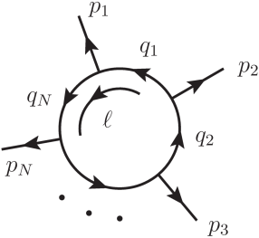
Figure 1: Generic one-loop topology with $N$ external legs.

On the other hand, the $d$-dimensional loop measure is given by

$$\int_{\ell}\bullet=-\imath\mu^{4-d}\int\frac{d^{d}\ell}{(2\pi)^{d}}\bullet~{}\,,$$ (5)

and

$$\tilde{\delta}\left(q_{i}\right)\equiv 2\pi\,\imath\,\theta(q_{i,0})\,\delta(q_{i}^{2}-m_{i}^{2})\,$$ (6)

used in Eq. (2) set the internal lines on-shell. It is worth mentioning that, the presence of the Heaviside function restricts the integration domain to the positive energy region (i.e. $q_{i,0}>0$). Since LTD is derived through the application of the Cauchy’s residue theorem, the remaining $d-1$ dimensional integration is performed over the forward on-shell hyperboloids defined by the solution of $G_{F}(q_{i})^{-1}=0$ with $q_{i,0}>0$. Notice that these on-shell hyperboloids degenerate to light-cones when internal particles are massless.

The dual representation shown in Eq. (2) is built by adding all possible single-cuts from the original loop diagram. In this procedure, the propagator associated with the on-shell line is replaced by Eq. (6) where the remaining uncut Feynman propagators are promoted to dual ones. The introduction of dual propagators modifies the $\imath 0$-prescription since it depends on the sign of $\eta\cdot k_{ji}$, with $\eta$ a future-like vector, $\eta^{2}\geq 0$, with positive definite energy $\eta_{0}>0$, and $k_{ji}$, which is independent of the loop momentum $\ell$ at one-loop. According to the derivation shown in Ref. [23], $\eta$ is arbitrary so we can chose $\eta_{\mu}=(1,{\bf 0})$ to simplify the implementation.

The difference between LTD and the Feynman Tree Theorem (FTT) [24, 25], where the loop integral is obtained after summing over all possible $m$-cuts, is codified in the dual prescription, where correlations coming from multiple cuts in the FTT are recovered in the LTD by considering only single-cuts with the modified $\imath 0$-prescription. In other words, having different prescriptions for each cut is a necessary condition for the consistency of the method. As discussed in Ref. [26], the integrand in Eq. (2) becomes singular at the intersection of forward on-shell hyperboloids (FF case), and forward with backward ($q_{j,0}<0$) on-shell hyperboloids (FB intersections). On one hand, the FF singularities cancel each other among different dual contributions; the change of sign in the modified prescription is crucial to enable this behaviour. On the other hand, singularities associated with FB intersections remain constrained to a compact region of the loop three-momentum space and are easily reinterpreted in terms of causality.

From a physical point of view, FB singularities take place when the on-shell virtual particle interacts with another on-shell virtual particle after the emission of outgoing on-shell radiation. The direction of the internal momentum flow establishes a natural causal ordering, and this interpretation is consistent with the Cutkosky rule. In fact, the total energy of the emitted particles, which is equal to $q_{i,0}-|q_{j,0}|$, has to be positive. Together with the positive energy constraint imposed by the delta distribution in Eq. (6), it restricts the possible kinematical configurations compatible with a sequential decay of on-shell physical particles.

Besides the mathematical understanding of the origin of the singularities by using the LTD, one of the most promising applications is the possible computation of scattering processes at NLO directly in four space-time dimensions without Dimensional Regularization (DREG). It has been also shown in Ref.[27] that one of the ingredients in order to build the 4D integrals are the renormalization constants. In fact, even if some integrals vanish at integral level, they are important for the local cancellation of singularities and the definition of renormalizad quantities in the LTD formalism. Therefore, in the next sections we compute the QED and QCD self-energy corrections by using the LTD theorem.

3 Photon and electron self-energies in QED

In the framework of QED, we need to compute the renormalization constants of the photon and the electron self-energies. In this handwritten, we will work in the massless approximation, labelling the internal lines as $q_{1}=\ell$, $q_{2}=\ell+p$ and considering $p^{2}\not=0$.

3.1 Photon self-energy

The one-loop photon self-energy is given by

$$\imath\,\Pi_{\mu\nu}(p^{2})=-\int_{\ell}{\mbox{Tr}}\left[\imath e_{0}\gamma_{\mu}\left(\imath\frac{q/_{1}+m_{0}}{q_{1}^{2}-m_{0}^{2}+\imath 0}\right)\imath e_{0}\gamma_{\nu}\left(\imath\frac{q/_{2}+m_{0}}{q_{2}^{2}-m_{0}^{2}+\imath 0}\right)\right]\,,$$ (7)

where due to gauge invariance

$$\Pi_{\mu\nu}(p^{2})=(p^{2}\,g_{\mu\nu}-p_{\mu}p_{\nu})\Pi(p^{2})\,.$$ (8)

From Eq. (7) and Eq. (8) and taking the massless approximation,

$$\imath(p^{2}\,g_{\mu\nu}-p_{\mu}p_{\nu})\Pi(p^{2})=-e_{0}^{2}\int_{\ell}\frac{\mbox{Tr}\left[\gamma_{\mu}\,q/_{1}\,\gamma_{\nu}\,q/_{2}\right]}{(q_{1}^{2}+\imath 0)\,(q_{2}^{2}+\imath 0)}\,.$$ (9)

Contracting Eq. (10) with the metric tensor in d-dimensions we can extract the scalar function as,

$$\Pi(p^{2})=\frac{8\,(1-\epsilon)\,e_{0}^{2}}{(3-2\epsilon)\,p^{2}}\int_{\ell}\,\frac{q_{1}\cdot q_{2}}{(q_{1}^{2}+\imath 0)\,(q_{2}^{2}+\imath 0)}\,.$$ (10)

Applying the LTD to the integral in Eq. (10)  ,

$$\Pi(p^{2}) = -\frac{8\,(1-\epsilon)\,e_{0}^{2}}{(3-2\epsilon)\,p^{2}}\,\left[\int_{\ell}\tilde{\delta}(q_{1})\frac{p\cdot q_{1}}{2p\cdot q_{1}+p^{2}-\imath 0}-\int_{\ell}\tilde{\delta}(q_{2})\frac{p\cdot q_{2}}{-2p\cdot q_{2}+p^{2}+\imath 0}\right]\,,$$ (11)

and taking the parametrization

$$p^{\mu} = (p_{0},{\bf 0})\,,$$

$$q_{i}^{\mu} = p_{0}\xi_{i,0}\left(1,2\sqrt{v_{i}(1-v_{i})}{\bf e}_{i,\perp},1-2v_{i}\right)\,,$$

$$\Pi(p^{2})=-\frac{2^{5}\,(1-\epsilon)\,e_{0}^{2}}{(3-2\epsilon)}\,\left[\int d[\xi_{1,0}]d[v_{1}]\frac{\xi^{2}_{1,0}}{1+2\xi_{1,0}-\imath 0}-\int d[\xi_{2,0}]d[v_{2}]\frac{\xi^{2}_{2,0}}{1-2\xi_{2,0}+\imath 0}\right]\,,$$ (13)

where

$$d[\xi_{i,0}]=\frac{(4\pi)^{\epsilon-2}}{\Gamma(1-\epsilon)}\left(\frac{4p^{2}}{\mu^{2}}\right)^{-\epsilon}\xi_{i,0}^{-2\epsilon}d\xi_{i,0}\quad{\rm and}\quad d[v_{i}]=(v_{i}(1-v_{i}))^{-\epsilon}dv_{i}\,.$$ (14)

The parameters $\xi_{i,0}$ and $v_{i}$ describe the energy and polar angle of the loop momentum respectively, defined in the regions $\xi_{i,0}\in[0,\infty)$ and $v_{i}\in[0,1]$. In order to explore the singular behaviour of $\Pi(p^{2})$, we integrate Eq. (13) over the regions $i)\,\xi_{i}\in[0,\omega]$ and $ii)\,\xi_{i}\in[\omega,\infty)$. After integration, we found:

$$\Pi(p^{2};\xi_{i}\leq\omega)=-\frac{4\,e_{0}^{2}\,S_{\epsilon}}{3}\left[4\,\omega^{2}+\log(1+2\,\omega-\imath 0)+\log(1-2\,\omega+\imath 0)\right]+O(\epsilon)\,$$ (15)

and

$$\Pi(p^{2};\xi_{i}\geq\omega)=-\frac{4\,e_{0}^{2}\,S_{\epsilon}}{3}\left[\frac{1}{\epsilon}-4\,\omega^{2}-\log(1+2\,\omega-\imath 0)-\log(1-2\,\omega+\imath 0)+\frac{5}{3}\right]+O(\epsilon)\,,$$ (16)

where $S_{\epsilon}=\frac{(4\pi)^{-2+\epsilon}}{\Gamma(1-\epsilon)\mu^{-2\epsilon}}(-p^{2}-\imath 0)^{-\epsilon}$. From these results, it is clear that IR divergences are absent. Besides, $\Pi(p^{2};\xi_{i}\leq\omega)$ is finite while the ultraviolet (UV) divergence is located fully in $\Pi(p^{2};\xi_{i}\geq\omega)$ . Since $\Pi(p^{2};\xi_{i}\leq\omega)$ is IR finite, it admits a four dimensional integrand realization given by,

$$\Pi(p^{2};\xi_{i}\leq\omega)=-\frac{e_{0}^{2}}{6\pi^{2}}\int_{0}^{1}dv_{1}\int_{0}^{\omega}\frac{d\xi_{1,0}\,4\xi_{1,0}^{2}}{1+2\xi_{1,0}-\imath 0}\left[1+\log\left(\xi_{1,0}^{2}\right)\left(v_{1}\delta\left(v_{1}\right)+\left(1-v_{1}\right)\delta\left(1-v_{1}\right)\right)\right]$$

$$+\frac{e_{0}^{2}}{6\pi^{2}}\int_{0}^{1}dv_{2}\int_{0}^{\omega}\frac{d\xi_{2,0}\,4\xi_{2,0}^{2}}{1-2\xi_{2,0}+\imath 0}\left[1+\log\left(\xi_{2,0}^{2}\right)\left(v_{2}\delta\left(v_{2}\right)+\left(1-v_{2}\right)\delta\left(1-v_{2}\right)\right)\right],$$ (17)

where the presence of the logarithmic terms are originated from the fact that we are using different coordinate systems for each dual integral.

The previous results shows one of the central implications of the use of the LTD theorem, resides in the location of singularities in physical regions. Hence, segmenting the integration domain, it is possible to find regions where the $\epsilon$-parameter is no longer needed. It is also worth to highlight that in Eq. (17) is showing explicitly the cut dependency, this fact will be relevant when a physical process with photons is calculated at NLO accuracy.

3.2 Electron self-energy

The one-loop electron self-energy is given by

$$-\imath\Sigma(p)=\int_{\ell}\imath e_{0}\gamma^{\mu}\left(\imath\frac{q/_{2}+m}{q_{2}^{2}-m_{0}^{2}+\imath 0}\right)\imath e_{0}\gamma^{\nu}\frac{-\imath}{q_{1}^{2}+\imath 0}g_{\mu\nu}\,,$$ (18)

where

$$\Sigma(p)=p/\Sigma_{V}(p^{2})-m\Sigma_{S}(p^{2})\,.$$ (19)

Considering Eq. (18), Eq. (19) and the massless case, we get,

$$-\imath\,p/\,\Sigma_{V}(p^{2})=-e_{0}^{2}\int_{\ell}\frac{\gamma^{\mu}q/_{2}\gamma_{\mu}}{(q_{1}^{2}+\imath 0)(q_{2}^{2}+\imath 0)}\,.$$ (20)

Extracting the scalar function $\Sigma_{V}(p^{2})$, we find,

$$\Sigma_{V}(p^{2}) = -2\,(1-\epsilon)\,e_{0}^{2}\int_{\ell}\,\frac{1}{(q_{1}^{2}+\imath 0)\,(q_{2}^{2}+\imath 0)}\left(1+\frac{p\cdot q_{2}}{p^{2}}\right)\,.$$ (21)

Then, applying the LTD,

$$\Sigma_{V}(p^{2}) = 2(1-\epsilon)\,e_{0}^{2}\left(\int_{\ell}\frac{\tilde{\delta}(q_{1})}{2p\cdot q_{1}+p^{2}-\imath 0}\left(1+\frac{p\cdot q_{1}}{p^{2}}\right)+\frac{1}{p^{2}}\int_{\ell}\frac{\tilde{\delta}(q_{2})\,p\cdot q_{2}}{-2p\cdot q_{2}+p^{2}+\imath 0}\right)\,,$$ (22)

working with the parametrization defined in Eq. (LABEL:parameters), $\Sigma_{V}(p^{2})$ becomes,

$$\Sigma_{V}(p^{2}) = 2(1-\epsilon)\,e_{0}^{2}\left(\int d[\xi_{1,0}]d[v_{1}]\frac{4\xi_{1,0}\left(1+\xi_{1,0}\right)}{1+2\xi_{1,0}-\imath 0}+\int d[\xi_{2,0}]d[v_{2}]\frac{4\xi_{2,0}^{2}}{1-2\xi_{2,0}+\imath 0}\right)\,.$$ (23)

To explore the behaviour of singularities from $\Sigma_{V}(p^{2})$, we segment the integration region similar to the photon propagator case. Computing the integrals in both regions, we find,

$$\Sigma_{V}(p^{2};\xi_{i}\leq\omega)=e_{0}^{2}\,S_{\epsilon}\left[-\log(1+2\omega-\imath 0)-\log(1-2\omega+\imath 0)\right]+O\left(\epsilon\right)\,,$$ (24)

$$\Sigma_{V}(p^{2};\xi_{i}\geq\omega)=e_{0}^{2}\,S_{\epsilon}\left[-\frac{1}{\epsilon}+\log(1+2\omega-\imath 0)+\log(1-2\omega+\imath 0)-1\right]+O(\epsilon)\,.$$ (25)

Based on these we find that $\Sigma_{V}(p^{2})$ has not IR divergence and similar conclusions to the photon propagator case can be inferred. Since $\Sigma_{V}(p^{2};\xi_{i}\leq\omega)$ is finite, we found that,

$$\Sigma_{V}(p^{2};\xi_{i}\leq\omega)=\frac{e_{0}^{2}}{8\pi^{2}}\int_{0}^{1}dv_{1}\int_{0}^{\omega}\,d\xi_{1,0}\frac{4\xi_{1,0}\left(1+\xi_{1,0}\right)}{1+2\xi_{1,0}-\imath 0}\left[1+\log\left(\xi_{1,0}^{2}\right)\left[v_{1}\delta\left(v_{1}\right)+\left(1-v_{1}\right)\delta\left(1-v_{1}\right)\right]\right]$$

$$+\frac{e_{0}^{2}}{8\pi^{2}}\int_{0}^{1}dv_{2}\int_{0}^{\omega}\,d\xi_{2,0}\frac{4\xi_{2,0}^{2}}{1-2\xi_{2,0}+\imath 0}\left[1+\log\left(\xi_{2,0}^{2}\right)\left[v_{2}\delta\left(v_{2}\right)+\left(1-v_{2}\right)\delta\left(1-v_{2}\right)\right]\right]\,,$$ (26)

is a four dimensional representation of it. It is worth mentioning that the massive case has been studied in Ref.[28], but in this work we are only focused in the one-loop self-energies corrections to massless propagators.

4 Quark and gluon self-energies in QCD

In this section we explicitly compute the quark and gluon self-energy corrections at one-loop in QCD.

4.1 Quark self-energy

One loop correction to the quark self-energy has a similar structure to the electron propagator in QED. The one-loop quark self-energy differs from the one-loop electron self-energy, only by the replacement of $e_{0}$ by $g_{0}$ and the inclusion of the colour factor $C_{F}$.

Then, we have that the scalar function $\Sigma_{V}(p^{2})$ is finite in the region $[0,\omega)$ and has a pole related to the presence of UV divergence at $[\omega,\infty]$. As in the electron case, there is a four dimensional realization given by

$$\Sigma_{V}(p^{2};\xi_{i}\leq\omega) = \frac{C_{F}\,g_{0}^{2}}{8\pi^{2}}\int_{0}^{1}dv_{1}\int_{0}^{\omega}\,d\xi_{1,0}\frac{4\xi_{1,0}\left(1+\xi_{1,0}\right)}{1+2\xi_{1,0}-\imath 0}\left[1+\log\left(\xi_{1,0}^{2}\right)\left[v_{1}\delta\left(v_{1}\right)+\left(1-v_{1}\right)\delta\left(1-v_{1}\right)\right]\right]$$

$$+ \frac{C_{F}\,g_{0}^{2}}{8\pi^{2}}\int_{0}^{1}dv_{2}\int_{0}^{\omega}\,d\xi_{2,0}\frac{4\xi_{2,0}^{2}}{1-2\xi_{2,0}+\imath 0}\left[1+\log\left(\xi_{2,0}^{2}\right)\left[v_{2}\delta\left(v_{2}\right)+\left(1-v_{2}\right)\delta\left(1-v_{2}\right)\right]\right].$$

4.2 Gluon self-energy

We analyse now the one-loop QCD correction to the gluon self-energy (in the Feynman gauge), which receives three different contributions, the quark, the gluon and the ghost-loop. For the gluon self-energy, the one-loop scalar function can be written as:

$$\Pi(p^{2})=\Pi_{q}(p^{2})+\Pi_{1}(p^{2})+\Pi_{2}(p^{2})\,,$$ (28)

where $\Pi_{q}(p^{2})$, $\Pi_{1}(p^{2})$ and $\Pi_{2}(p^{2})$ are the corresponding scalar functions belonging to the quark, the gluon and the ghost-loop, respectively.

The quark-loop contribution differs from the one-loop photon self-energy only by the replacement of $e_{0}$ by $g_{0}$ and the inclusion of the factor $n_{f}$, representing the number of fermions in the loop, therefore;

$$\Pi_{q}(p^{2}) = \frac{8\,n_{f}\,(1-\epsilon)\,g_{0}^{2}}{(3-2\epsilon)\,p^{2}}\int_{\ell}\,\frac{q_{1}\cdot q_{2}}{(q_{1}^{2}+\imath 0)\,(q_{2}^{2}+\imath 0)}\,.$$ (29)

Now, the contribution coming from the gluon-loop is

$$\Pi_{1}(p^{2}) = -\frac{\imath\,C_{A}g_{0}^{2}}{2(3-2\epsilon)\,p^{2}}\int_{\ell}\frac{N}{(q_{1}^{2}+\imath 0)\,(q_{2}^{2}+\imath 0)}\,,$$ (30)

where the numerator is

$$N = d((q_{1}+q_{2})^{2}+(2q_{1}-q_{2})^{2}+(2q_{2}-q_{1})^{2})$$ (31)

$$- 2(q_{1}+q_{2})\cdot(2q_{1}-q_{2})-2q_{2}\cdot(2q_{2}-q_{1})+2(2q_{2}-q_{1})\cdot(2q_{1}-q_{2})\,.$$

Applying the LTD to the integral in Eq. (30) , we find,

$$\Pi_{1}(p^{2})=-3\,C_{A}\,g_{0}^{2}\left(\int_{\ell}\frac{\tilde{\delta}(q_{1})}{p^{2}+2p\cdot q_{1}-\imath 0}\left(1+\frac{p\cdot q_{1}}{p^{2}}\right)+\int_{\ell}\frac{\tilde{\delta}(q_{2})}{p^{2}-2p\cdot q_{2}+\imath 0}\left(1-\frac{p\cdot q_{1}}{p^{2}}\right)\right)\,.$$ (32)

Using the same parametrization, we find,

$$\Pi_{1}(p^{2}) = -\frac{12\,C_{A}\,g_{0}^{2}}{\Gamma(2-2\epsilon)}\left(\int d[v_{1}]\,d[\xi_{1,0}]\frac{\xi_{1,0}\,(1+\xi_{1,0})}{1+2\xi_{1,0}-\imath 0}+\int d[v_{2}]\,d[\xi_{2,0}]\frac{\xi_{2,0}\,(1-\xi_{2,0})}{1-\xi_{2,0}+\imath 0}\right)\,.$$ (33)

Similar to the QED results, we find after integration

$$\Pi_{1}(p^{2};\xi_{i}\leq\omega)=\frac{C_{A}\,g_{0}^{2}\,S_{\epsilon}}{3}\left[4\omega^{2}-\log\left(1+2\omega-\imath 0\right)-\log\left(1-2\omega+\imath 0\right)\right]+O(\epsilon)\,,$$ (34)

$$\Pi_{1}(p^{2};\xi_{i}\geq\omega)=\frac{C_{A}\,g_{0}^{2}\,S_{\epsilon}}{3}\left[-\frac{1}{\epsilon}-4\omega^{2}+\log\left(1+2\omega-\imath 0\right)+\log\left(1-2\omega+\imath 0\right)-\frac{4}{3}\right]+O\left(\epsilon\right).$$ (35)

Therefore, the four dimensional representation of $\Pi_{1}(p^{2};\xi_{i}\leq\omega)$ is given by,

$$\Pi_{1}(p^{2};\xi_{i}\leq\omega) = -\frac{9C_{A}g_{0}^{2}}{4\pi^{2}}\int_{0}^{1}dv_{1}\int_{0}^{\omega}\frac{d\xi_{1,0}\xi_{1,0}\left(1+\xi_{1,0}\right)}{1+2\xi_{1,0}-\imath 0}[1+\log\left(\xi_{1,0}^{2}\right)\left[v_{1}\delta\left(v_{1}\right)+\left(1-v_{1}\right)\delta\left(1-v_{1}\right)\right]]$$

$$- \frac{9C_{A}g_{0}^{2}}{4\pi^{2}}\int_{0}^{1}dv_{2}\int_{0}^{\omega}\frac{d\xi_{2,0}\xi_{2,0}\left(1-\xi_{2,0}\right)}{1-2\xi_{2,0}+\imath 0}[1+\log\left(\xi_{2,0}^{2}\right)\left[v_{2}\delta\left(v_{2}\right)+\left(1-v_{2}\right)\delta\left(1-v_{2}\right)\right]]\,.$$

The last remaining piece is due to the ghost-loop, the interested integral is given by,

$$\Pi_{2}(p^{2}) = \frac{\imath\,C_{A}\,g_{0}^{2}}{(3-2\epsilon)p^{2}}\int_{\ell}\frac{q_{1}\cdot q_{2}}{(q_{1}^{2}+\imath 0)\,(q_{2}^{2}+\imath 0)}$$ (37)

applying LTD to the previous expression,

$$\Pi_{2}(p^{2}) = \frac{C_{A}\,g_{0}^{2}}{(3-2\epsilon)p^{2}}\left(\int_{\ell}\frac{\tilde{\delta}(q_{1})q_{1}\cdot p}{p^{2}+2p\cdot q_{1}-\imath 0}-\int_{\ell}\frac{\tilde{\delta}(q_{2})p\cdot q_{2}}{p^{2}-2p\cdot q_{2}+\imath 0}\right)\,,$$ (38)

Following the precedent ideas, we find that the integral is decomposed as

$$\Pi_{2}(p^{2};\xi_{i}\leq\omega)=\frac{C_{A}g_{0}^{2}\,S_{\epsilon}}{3}\left[4\omega^{2}+\log\left(1+2\omega-\imath 0\right)+\log\left(1-2\omega+\imath 0\right)\right]+O\left(\epsilon\right)\,,$$ (39)

$$\Pi_{2}(p^{2};\xi_{i}\geq\omega)=\frac{C_{A}g_{0}^{2}\,S_{\epsilon}}{3}\left[\frac{1}{\epsilon}-4\omega^{2}-\log\left(1+2\omega-\imath 0\right)-\log\left(1-2\omega+\imath 0\right)+2\right]+O\left(\epsilon\right)\,.$$ (40)

Finally, we find that the four dimensional representation of $\Pi_{2}(p^{2};\xi_{i}\leq\omega)$ is given by

$$\Pi_{2}(p^{2};\xi_{i}\leq\omega) = \frac{C_{A}g_{0}^{2}}{48\pi^{2}}\int_{0}^{1}dv_{1}\int_{0}^{\omega}\frac{d\xi_{1,0}4\xi_{1,0}^{2}}{1+2\xi_{1,0}-\imath 0}\left[1+\log\left(\xi_{1,0}^{2}\right)\left[v_{1}\delta\left(v_{1}\right)+\left(1-v_{1}\right)\delta\left(1-v_{1}\right)\right]\right]$$ (41)

$$+ \frac{C_{A}g_{0}^{2}}{48\pi^{2}}\int_{0}^{1}dv_{2}\int_{0}^{\omega}\frac{d\xi_{2,0}4\xi_{2,0}^{2}}{1-2\xi_{2,0}+\imath 0}\left[1+\log\left(\xi_{2,0}^{2}\right)\left[v_{2}\delta\left(v_{2}\right)+\left(1-v_{2}\right)\delta\left(1-v_{2}\right)\right]\right]$$

Gathering the four dimensional representations of the three different contributions to the gluon self-energy, the quark, the gluon and the ghost loop, we have that the four dimensional realization of $\Pi(p^{2};\xi_{i}\leq\omega$) is given by,

$$\Pi(p^{2};\xi_{i}\leq\omega)=\Pi_{q}(p^{2};\xi_{i}\leq\omega)+\Pi_{1}(p^{2};\xi_{i}\leq\omega)+\Pi_{2}(p^{2};\xi_{i}\leq\omega)\,.$$ (42)

5 Conclusions

In this paper we have shown that working with the LTD method the scalars functions from the one-loop self energies present only simple poles related to their UV-singular behaviour. Therefore a purely four dimensional representation could be always found for a region belonging to the $\omega$-cut in the energy component. The possibility to obtain a four dimensional realization implies a major improvement in the computation of higher-order corrections in QFT, besides, allows a better understanding of the mathematical structures behind scattering amplitudes.

6 Acknowledgment

This work is supported by CONACyT, Mexico, PROFAPI 2015 grant number 121 and DPyC, by the Spanish Government and ERDF funds from European Commission (Grants No. FPA2014-53631-C2-1-P and SEV-2014-0398) and by Consejo Superior de Investigaciones Científicas (Grant No. PIE-201750E021)

7 References

References

• [1] Z. Kunszt and D. E. Soper, “Calculation of jet cross-sections in hadron collisions at order alpha-s**3,” Phys. Rev. D 46 (1992) 192.
• [2] S. Frixione, Z. Kunszt and A. Signer, “Three jet cross-sections to next-to-leading order,” Nucl. Phys. B 467 (1996) 399 [hep-ph/9512328].
• [3] S. Catani and M. H. Seymour, “The Dipole formalism for the calculation of QCD jet cross-sections at next-to-leading order,” Phys. Lett. B 378 (1996) 287 [hep-ph/9602277].
• [4] S. Catani and M. H. Seymour, “A General algorithm for calculating jet cross-sections in NLO QCD,” Nucl. Phys. B 485 (1997) 291 [Nucl. Phys. B 510 (1998) 503] [hep-ph/9605323].
• [5] A. Gehrmann-De Ridder, T. Gehrmann and E. W. N. Glover, “Antenna subtraction at NNLO,” JHEP 0509 (2005) 056 [hep-ph/0505111].
• [6] S. Catani and M. Grazzini, “An NNLO subtraction formalism in hadron collisions and its application to Higgs boson production at the LHC,” Phys. Rev. Lett.  98 (2007) 222002 [hep-ph/0703012].
• [7] M. Czakon, “A novel subtraction scheme for double-real radiation at NNLO,” Phys. Lett. B 693 (2010) 259 [arXiv:1005.0274 [hep-ph]].
• [8] P. Bolzoni, G. Somogyi and Z. Trocsanyi, “A subtraction scheme for computing QCD jet cross sections at NNLO: integrating the iterated singly-unresolved subtraction terms,” JHEP 1101 (2011) 059 [arXiv:1011.1909 [hep-ph]].
• [9] V. Del Duca, C. Duhr, G. Somogyi, F. Tramontano and Z. Trócsányi, “Higgs boson decay into b-quarks at NNLO accuracy,” JHEP 1504 (2015) 036 [arXiv:1501.07226 [hep-ph]].
• [10] R. Boughezal, C. Focke, X. Liu and F. Petriello, “$W$-boson production in association with a jet at next-to-next-to-leading order in perturbative QCD,” Phys. Rev. Lett.  115 (2015) 062002 [arXiv:1504.02131 [hep-ph]].
• [11] J. Gaunt, M. Stahlhofen, F. J. Tackmann and J. R. Walsh, “N-jettiness Subtractions for NNLO QCD Calculations,” JHEP 1509 (2015) 058 [arXiv:1505.04794 [hep-ph]].
• [12] R. A. Fazio, P. Mastrolia, E. Mirabella, W. J. Torres-Bobadilla, “On the four-dimensional formulation of dimensionally regulated amplitudes,” Eur. Phys. J.C. 74 (2014) 3197
• [13] G. Rodrigo, S. Catani, T. Gleisberg, F. Krauss and J. C. Winter, “From multileg loops to trees (by-passing Feynman’s Tree Theorem),” Nucl. Phys. Proc. Suppl.  183 (2008) 262 [arXiv:0807.0531 [hep-th]].
• [14] I. Bierenbaum, S. Catani, P. Draggiotis and G. Rodrigo, “A Tree-Loop Duality Relation at Two Loops and Beyond,” JHEP 1010 (2010) 073 [arXiv:1007.0194 [hep-ph]].
• [15] I. Bierenbaum, S. Buchta, P. Draggiotis, I. Malamos and G. Rodrigo, “Tree-Loop Duality Relation beyond simple poles,” JHEP 1303 (2013) 025 [arXiv:1211.5048 [hep-ph]].
• [16] I. Bierenbaum, P. Draggiotis, S. Buchta, G. Chachamis, I. Malamos and G. Rodrigo, “News on the loop–tree Duality,” Acta Phys. Polon. B 44 (2013) 2207.
• [17] S. Buchta, “Theoretical foundations and applications of the Loop-Tree Duality in Quantum Field Theories,” PhD thesis, Universitat de València, 2015, arXiv:1509.07167 [hep-ph].
• [18] S. Buchta, G. Chachamis, P. Draggiotis, I. Malamos and G. Rodrigo, “Towards a Numerical Implementation of the Loop-Tree Duality Method,” Nucl. Part. Phys. Proc.  258-259 (2015) 33 [arXiv:1509.07386 [hep-ph]].
• [19] S. Buchta, “First Numerical Implementation of the Loop-Tree Duality Method,” PoS EPS-HEP 2015 (2015) 430 [arXiv:1510.04105 [hep-ph].
• [20] S. Buchta, G. Chachamis, P. Draggiotis and G. Rodrigo, “Numerical implementation of the Loop-Tree Duality method,” arXiv:1510.00187 [hep-ph].
• [21] R. J. Hernández-Pinto, G. F. R. Sborlini and G. Rodrigo, “Towards gauge theories in four dimensions,” JHEP 1602 (2016) 044 [arXiv:1506.04617 [hep-ph]].
• [22] G. F. R. Sborlini, “Loop-tree duality and quantum field theory in four dimensions,” PoS RADCOR 2015 (2015) 082 [arXiv:1601.04634 [hep-ph]].
• [23] S. Catani, T. Gleisberg, F. Krauss, G. Rodrigo and J. C. Winter, “From loops to trees by-passing Feynman’s theorem,” JHEP 0809 (2008) 065 [arXiv:0804.3170 [hep-ph]].
• [24] R. P. Feynman, “Quantum theory of gravitation,” Acta Phys. Polon.  24 (1963) 697.
• [25] R. P. Feynman, “Closed Loop And Tree Diagrams. (talk),” In *Brown, L.M. (ed.): Selected papers of Richard Feynman* 867-887
• [26] S. Buchta, G. Chachamis, P. Draggiotis, I. Malamos and G. Rodrigo, “On the singular behaviour of scattering amplitudes in quantum field theory,” JHEP 1411 (2014) 014 [arXiv:1405.7850 [hep-ph]].
• [27] G. F. R. Sborlini, R. Hernández-Pinto and G. Rodrigo, “From dimensional regularization to NLO computations in four dimensions,” PoS EPS-HEP 2015 (2015) 479 [arXiv:1510.01079 [hep-ph]].
• [28] G. F. R. Sborlini, Felix Driencourt-Mangin, German Rodrigo “Four-dimensional unsubtraction with massive particles,” JHEP 1610 (2016) 162 [arXiv:1608.01584 [hep-ph]].