The GENIUS Approach to Robust Mendelian Randomization Inference

Abstract

Mendelian randomization (MR) is a popular instrumental variable (IV) approach, in which one or several genetic markers serve as IVs that can sometimes be leveraged to recover valid inferences about a given exposure-outcome causal association subject to unmeasured confounding. A key IV identification condition known as the exclusion restriction states that the IV cannot have a direct effect on the outcome which is not mediated by the exposure in view. In MR studies, such an assumption requires an unrealistic level of prior knowledge about the mechanism by which genetic markers causally affect the outcome. As a result, possible violation of the exclusion restriction can seldom be ruled out in practice. To address this concern, we introduce a new class of IV estimators which are robust to violation of the exclusion restriction under data generating mechanisms commonly assumed in MR literature. The proposed approach named ”MR G-Estimation under No Interaction with Unmeasured Selection” (MR GENIUS) improves on Robins’ G-estimation by making it robust to both additive unmeasured confounding and violation of the exclusion restriction assumption. In certain key settings, MR GENIUS reduces to the estimator of Lewbel (2012) which is widely used in econometrics but appears largely unappreciated in MR literature. More generally, MR GENIUS generalizes Lewbel’s estimator to several key practical MR settings, including multiplicative causal models for binary outcome, multiplicative and odds ratio exposure models, case control study design and censored survival outcomes.

, and

1 Introduction

Mendelian randomization (MR) is an instrumental variable approach with growing popularity in epidemiology studies. In MR, one aims to establish a causal association between a given exposure and an outcome of interest in the presence of possible unmeasured confounding, by leveraging one or more genetic markers defining the IV (Davey Smith and Ebrahim, 2003, 2004; Lawlor et al., 2008). In order to be a valid IV, a genetic marker must satisfy the following key conditions:

(a)

It must be associated with the exposure.

(b)

It must be independent of any unmeasured confounder of the exposure-outcome relationship.

(c)

There must be no direct effect of the genetic marker on the outcome which is not fully mediated by the exposure in view.

Assumption (c) also known as the exclusion restriction is rarely credible in the context of MR as it requires complete understanding of the biological mechanism by which each marker influences the outcome. Such a priori knowledge may be unrealistic in practice due to the possible existence of unknown pleiotropic effects of the markers (Little and Khoury, 2003; Davey Smith and Ebrahim, 2003, 2004; Lawlor et al., 2008). Violation of assumption (b) can also occur due to linkage disequilibrium or population stratification (Lawlor et al., 2008). Possible violation or near violation of assumption (a) known as the weak instrumental variable problem also poses an important challenge in MR as individual genetic effects on phenotypes can be fairly weak.

There has been tremendous interest in the development of statistical methods to detect and account for violation of IV assumptions (a)–(c), primarily in multiple-IV settings under standard linear outcome and exposure models. The literature addressing violation of assumption (a) is arguably the most developed and extends to possible nonlinear models under a generalized methods of moments framework; notable papers of this rich literature include Staiger and Stock (1997), Stock and Wright (2000), Stock, Wright and Yogo (2002), Chao and Swanson (2005) and Newey and Windmeijer (2009). Methodology to address violations of (b) or (c) is far less developed, and constitutes the central focus of this paper. Three strands of work stand out in recent literature concerning violation of either of these assumptions. In the first strand, Kang et al. (2016) developed a penalized regression approach that can recover valid inferences about the causal effect of interest provided fewer than fifty percent of genetic markers are invalid IVs (known as majority rule); Windmeijer et al. (2018) improved on the penalized approach, including a proposal for standard error estimation lacking in Kang et al. (2016). In an alternative approach, Han (2008) established that the median of multiple estimators of the effect of exposure obtained using one instrument at the time is a consistent estimator also assuming majority rule and that IVs cannot have direct effects on the outcome unless the IVs are uncorrelated. Bowden et al. (2016) explore closely related weighted median methodology. In a second strand of work, Guo et al. (2018) proposed two stage hard thresholding (TSHT) with voting, which is consistent for the causal effect under linear outcome and exposure models, and a plurality rule which can be considerably weaker than the majority rule. The plurality rule is defined in terms of regression parameters encoding the association of each invalid IV with the outcome and that encoding the association of the corresponding IV with the exposure. The condition effectively requires that the number of valid IVs is greater than the largest number of invalid IVs with equal ratio of the regression coefficients given above. Furthermore, they provide a simple construction for 95% confidence intervals to obtain inferences about the exposure effect which are guaranteed to have correct coverage under the plurality rule. Importantly, in these first two strands of work, a candidate IV may be invalid either because it violates the exclusion restriction, or because it shares an unmeasured common cause with the outcome, i.e. either (b) or (c) fails. Both the penalized approach and the median estimator may be inconsistent if majority rule fails, while TSHT may be inconsistent if plurality rule fails. For instance, it is clear that neither approach can recover valid inferences if all IVs violate either assumption (b) or (c). In a third strand of work, Kolesár et al. (2015) considered the possibility of identifying the exposure causal effect when all IVs violate the exclusion restriction (c), provided the effects of the IVs on the exposure are asymptotically orthogonal to their direct effects on the outcome as the number of IVs tends to infinity. A closely related meta-analytic version of their approach known as MR-Egger has recently emerged in the epidemiology literature (Bowden, Davey Smith and Burgess, 2015); they referred to the orthogonality condition as the instrument strength independent of direct effect (InSIDE) assumption. As pointed out by Kang et al. (2016), the orthogonality condition on which these approaches rely may be hard to justify in MR settings as it potentially restricts unknown pleiotropic effects of genetic markers often with little to no biological basis. A notable feature of aforementioned methods is that they are primarely tailored to a multiple-IV setting, in fact methods such as MR-Egger are consistent only under an asymptotic theory in which the number of IVs goes to infinity, together with sample size. It is also important to note that because confidence intervals for the causal effect of the exposure obtained by Windmeijer et al. (2018) and Guo et al. (2018) rely on a consistent model selection procedure, such confidence intervals fail to be uniformly valid over the entire model space (Guo et al., 2018; Leeb and Pötscher, 2008).

Because in practice, it is not possible to ensure that either majority rule or plurality rule holds, it is important to develop causal inference and estimation methods that are robust to possible violation of IV assumptions under alternative conditions. Lewbel (2012, 2018) proposed novel identification and estimation strategies with mismeasured and endogenous regressor models by leveraging a heteroscedastic covariance restriction, which has since been widely applied in econometrics and social sciences. In Section 2, we introduce notation used throughout and provide a review of the invalid IV model considered by Lewbel (2012). We extend Lewbel’s identification result in section 3. The proposed framework which we call ”MR G-Estimation under No Interaction with Unmeasured Selection” (MR GENIUS) can also be viewed as a version of Robins‘ G-estimation (Robins, 1994) that is robust to both additive unmeasured confounding and violation of IV assumptions, and which unlike the aforementioned methods equally applies whether one has observed a single or many candidate IVs. An important feature of multiple IV MR GENIUS is that the correlation structure for the IVs can essentially remain unrestricted without necessarily affecting identification, this is in contrast with Bowden, Davey Smith and Burgess (2015) who require uncorrelated IVs and Kang et al. (2016) who likewise require IV correlation structure to be somewhat restricted (Windmeijer et al., 2018). Section 4 presents several key generalizations including MR GENIUS under multiplicative or odds ratio exposure models, as well as for right censored time-to-event endpoint under a structural additive hazards model, which extends the recent semiparametric IV estimator of Martinussen et al. (2017) against possible violation of the exclusion restriction assumption. In section 5, we evaluate the proposed methods and compare them to a number of previous MR methods in extensive simulation studies. In section 6 we illustrate the methods in an MR analysis of the effect of diabetes on memory in the Health and Retirement Study. Section 7 offers some concluding remarks.

2 Notation and definitions

Suppose that one has observed $n$ i.i.d. realizations of a vector $(A,G,Y)$ where $A$ is an exposure, $G$ the candidate IV and $Y$ is the outcome. Let $U$ denote an unmeasured confounder (possibly multivariate) of the effect of $A$ on $Y.$ $G$ is said to be a valid instrumental variable provided it fulfills the following three conditions (Didelez, Meng and Sheehan, 2010):

Assumption 1.

IV relevance: $G\mathchoice{\mathrel{\hbox to0.0pt{\kern 7.63889pt\kern-5.27776pt$\displaystyle\not$\hss}{\perp\mkern-9.5mu\perp}}}{\mathrel{\hbox to0.0pt{\kern 7.63889pt\kern-5.27776pt$\textstyle\not$\hss}{\perp\mkern-9.5mu\perp}}}{\mathrel{\hbox to0.0pt{\kern 2.61118pt\kern-4.11108pt$\scriptstyle\not$\hss}{\perp\mkern-9.5mu\perp}}}{\mathrel{\hbox to0.0pt{\kern 1.11118pt\kern-3.3333pt$\scriptscriptstyle\not$\hss}{\perp\mkern-9.5mu\perp}}}A|U;$

Assumption 2.

IV independence: $G\perp\mkern-9.5mu\perp U;$

Assumption 3.

Exclusion restriction: $G\perp\mkern-9.5mu\perp Y|A,U.$

The first condition ensures that the IV is a correlate of the exposure even after conditioning on $U.$ The second condition states that the IV is independent of all unmeasured confounders of the exposure-outcome association, while the third condition formalizes the assumption of no direct effect of $G$ on $Y$ not mediated by $A$ (assuming Assumption 2 holds$)$.  The causal diagram in Figure 1a encodes these three assumptions and therefore provides a graphical representation of the IV model. It is well known that while a valid IV satisfying assumptions 1–3, i.e. the causal diagram in Figure 1a, suffices to obtain a valid statistical test of the sharp null hypothesis of no individual causal effect, the population average causal effect is itself not point identified with a valid IV without an additional assumption. In case of a valid binary IV and binary exposure, Wang and Tchetgen Tchetgen (2018) recently established that the average causal effect $\beta_{a}$ of $A$ on $Y$ is nonparametrically identified by the so-called Wald estimand

$$\beta_{a}=\delta\equiv\frac{E(Y|G=1)-E(Y|G=0)}{E(A|G=1)-E(A|G=0)},$$

if either of the conditions

$$E\left(Y|A,G,U\right)=\beta_{a}A+\beta_{u}\left(U\right)$$ (2.1)

$$E\left(A|G,U\right)=\alpha_{g}G+\alpha_{u}(U),$$ (2.2)

holds, where the unknown functions $\beta_{u}\left(\cdot\right)$ and $\alpha_{u}(\cdot)$ are restricted only by natural features of the model, e.g. such that the outcome and exposure means are bounded between zero and one in the binary case. Suppose that, as encoded in the diagram given in Figure 1b, assumption 3 does not necessarily hold. Lewbel (2012) considered identification and estimation of $\beta_{a}$ under the invalid IV model

$$E\left(Y|A,G,U\right) = \beta_{a}A+\beta_{g}(G)+\beta_{u}\left(U\right)$$ (2.3)

$$\quad E\left(A|G,U\right) = \alpha_{g}(G)+\alpha_{u}(U),$$ (2.4)

where $\beta_{g}(G)$ encodes the direct effect of $G$ on $Y$, with $\beta_{g}(0)=\alpha_{g}(0)=0$. Note that the models for $E(Y|A,G,U)$ and $E(A|G,U)$ considered by Bowden, Davey Smith and Burgess (2015) satisfy (2.3) with $\beta_{g}\left(\cdot\right)$ and $\alpha_{g}\left(\cdot\right)$ linear functions, while Kang et al. (2016) specified models implied by these two restrictions. With binary exposure $A$, we consider identification of the average causal effect for the following generalization of the invalid IV model considered in (2.3).

Assumption 4:

(4a)

For unknown functions $\beta_{g}\left(\cdot\right)$ and $\alpha_{g}(\cdot)$ of $(U,G)$ where $\beta_{g}\left(U,0\right)=\alpha_{g}(U,0)=0$, and unknown function $\beta_{a}(\cdot)$ of $U$,

$$E\left(Y|A,G,U\right) = \beta_{a}(U)A+\beta_{g}(U,G)+\beta_{u}\left(U\right)$$ (2.5)

$$E\left(A|G,U\right) = \alpha_{g}(U,G)+\alpha_{u}(U).$$ (2.6)

(4b)

The orthogonality conditions

$$\mbox{cov}\{\beta_{g}\left(U,G\right),\alpha_{g}(U,G)|G\}=\mbox{cov}\{\beta_{g}\left(U,G\right),\alpha_{u}(U)|G\}=0;$$

$$\mbox{cov}\{\beta_{a}(U),\alpha_{g}(U,G)|G\}=\mbox{cov}\{\beta_{a}(U),\alpha_{u}(U)|G\}=0;$$ (2.7)

$$\mbox{cov}\{\alpha_{g}(U,G),\beta_{u}\left(U\right)|G\}=0,$$

hold with probability 1.

Under assumption 4a, the average causal effect of binary $A$ on $Y$ is given by $E\{\beta_{a}(U)\}$. The model $\beta_{g}(U,G)$ encodes the direct effect of $G$ on $Y$, with potential effect modification by unmeasured confounders $U$. Assumption 4b does not imply orthogonality of $\beta_{u}(U)$ and $\alpha_{u}(U)$ and therefore the degree of unmeasured confounding is not restricted by these orthogonality conditions. In contrast the degree of common effect modifiers in the outcome and exposure models is effectively restricted by ((4b)). As a special case, the conditions in assumption 4b are satisfied if $\beta_{g}(U,G)=\beta_{g}(G)$, $\alpha_{g}(U,G)=\alpha_{g}(G)$ and $\beta_{a}(U)=\beta_{a}$ with probability 1, which is the scenario considered in Lewbel (2012). Assumption 4b may hold even if assumptions made by Lewbel (2012) do not, as illustrated by the following example. Suppose that $\alpha_{u}(U)-E[\alpha_{u}(U)]=\sum_{k=1}^{K}\gamma_{k}\times\phi_{k}(U)$ for a vector of zero-mean functions $\mathbf{\Phi}=\{\phi_{k}:k=1,..K\}$, and likewise $\beta_{u}(U)-E[\beta_{u}(U)]=\sum_{j=1}^{J}\theta_{j}\times\tau_{j}(U)$ for $\mathbf{T}=\{\tau_{j}:j=1,..J\}$. Denote the linear vector space spanned by the vector $\mathbf{\Omega}$ of functions in $U$ to be $S(\mathbf{\Omega})$, and $\Pi$ to be the least squares projection operator. Let

$$\alpha_{g}(U,G)=\alpha_{g0}(G)+\sum_{k=1}^{K}\alpha_{gk}(G)\{\phi_{k}(U)-\Pi[\phi_{k}(U)|S(\mathbf{T})]\},$$

$\alpha_{gk}(0)=0$ for $k=0,1,...,K$,

$$\beta_{g}(U,G)=\beta_{g0}(G)$$

$$+ \beta_{g1}(G)\{\omega(U)-\Pi[\omega(U)|S(\mathbf{\Phi})+S(\phi_{k}(U)-\Pi[\phi_{k}(U)|S(\mathbf{T})],k=1,2,...,K)]\},$$

for arbitrary function $\omega(U)$ with $\beta_{g0}(0)=\beta_{g1}(0)=0$, and

$$\beta_{a}(U)=\zeta(U)-\Pi[\zeta(U)|S(\mathbf{\Phi})+S(\phi_{k}(U)-\Pi[\phi_{k}(U)|S(\mathbf{T})],k=1,2,...,K)]$$

for arbitrary function $\zeta(U)$. Note that $\mathbf{\Phi}$ and $\mathbf{T}$ can be of different dimension. Then the orthogonality conditions of Assumption 4b are satisfied.

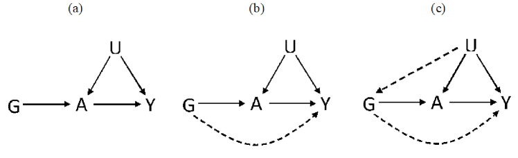
Figure 1: Directed acyclic graph depicting (a) a valid instrument $G$ which satisfies assumptions 1-3, (b) the situation in which exclusion restriction (assumption 3) does not necessarily hold (the dashed line indicates possible direct effect of $G$ on outcome $Y$), and (c) the situation in which IV independence (assumption 2) and exclusion restriction (assumption 3) do not necessarily hold (the dashed lines indicate possible direct effects of $U$ on $G$, and of $G$ on $Y$).

3 Identification and estimation under violation of exclusion restriction

We consider identification of $E\{\beta_{a}(U)\}$ within the large class of data generating mechanisms that satisfy assumptions 1, 2 and 4, which is given in the following lemma.

Lemma 3.1.

Suppose that Assumptions 1, 2 and 4 hold, then $E\{\beta_{a}(U)\}=\mu$, where

$$\mu \equiv \frac{E\left[\left\{G-E(G)\right\}\left\{A-E(A|G)\right\}Y\right]}{E\left[\left\{G-E(G)\right\}\left\{A-E(A|G)\right\}A\right]}$$

provided that

$$\phi\equiv\mbox{cov}\{G,\mbox{var}(A|G)\}\neq 0.$$ (3.1)

The proof for Lemma 3.1 is given in appendix A1 of the supplementary materials. In particular, for binary $G$, $\phi=var(G)\left\{var(A|G=1)-var(A|G=0)\right\}$ so that (3.1) is satisfied if and only if $\mbox{var}\left(A|G=1\right)-\mbox{var}\left(A|G=0\right)\neq 0$. Lemma 1 provides an explicit identifying expression for the average causal effect of $A$ on $Y$ in the presence of additive confounding, which leverages a candidate IV $G$ that may or may not satisfy the exclusion restriction. In order for $\mu$ to be well defined, we require a slight strengthening of the IV relevance assumption 1, i.e. that $var(A|G)$ must depend on $G$. It is key to note that this assumption is empirically testable, and will typically hold for binary $A$, other than at certain exceptional laws. To illustrate, let $\pi(g)=\Pr(A=1|G=g)$ and suppose that assumptions 1, 2 and 4 hold, however $\pi\left(1\right)=1-\pi\left(0\right),$ in which case $\left(\ref{strong IV}\right)$ fails because $var(A|G=g)=\pi(g)\left(1-\pi(g)\right)=\pi(1)\left(1-\pi(1)\right)=\pi(0)\left(1-\pi(0)\right)$ does not depend on $g$ and therefore the identifying expression given in the Lemma does not apply despite the candidate IV satisfying IV relevance assumption 1, i.e. $\pi\left(1\right)\not=\pi\left(0\right)$. Below, we extend Lemma 3.1 to allow for possible violation of both assumptions 2 and 3.

The lemma motivates the following MR estimator, which is guaranteed to be consistent under assumptions 1, 2, 4 and equation $\left(\ref{strong IV}\right)$ irrespective of whether or not assumption 3 also holds:

$$\widehat{\beta}_{a}=\frac{\mathbb{P}_{n}\left[\left\{G-\mathbb{P}_{n}(G)\right\}\left\{A-\widehat{E}(A|G)\right\}Y\right]}{\mathbb{P}_{n}\left[\left\{G-\mathbb{P}_{n}(G)\right\}\left\{A-\widehat{E}(A|G)\right\}A\right]},$$ (3.2)

where $\mathbb{P}_{n}=n^{-1}\sum_{i=1}^{n}[\cdot]_{i}$ and $\widehat{E}(A|G=g)=$ $\mathbb{P}_{n}\left[A_{i}1\left(G_{i}=g\right)\right]/\mathbb{P}_{n}\left[1\left(G_{i}=g\right)\right].$ This estimator is the simplest instance of MR GENIUS estimation. The asymptotic distribution of the estimator is described in appendix B1. We note that (3.2) is equivalent to Lewbel’s estimator which can be implemented as follows (Lewbel, 2018):

• Obtain the estimated residuals $\hat{\epsilon}_{a}=A-\hat{\theta}^{T}G$ from ordinary least squares regression of $A$ on $G$.

• Estimate $\beta_{a}$ by two-stage least squares regression of $Y$ on $A$, using $\left(G-\bar{G}\right)\hat{\epsilon}_{a}$ as the instrument, where $\bar{G}$ is the sample mean of $G$.

The above estimator assumes $E(A|G)=\theta^{T}G$, although the first step can be extended for some nonlinear, possibly unknown exposure model. Lewbel showed that $\hat{\beta}_{a}$ is consistent for the average causal effect which is parameterized by the scalar ${\beta}_{a}$ under model (2.3) and condition (3.1) as well as $\text{cov}\{G,{\epsilon}_{a}{\epsilon}_{y}\}=0,$ where ${\epsilon}_{y}=Y-\beta_{a}A$.

3.1 Continuous exposure

Consider the following stronger version of assumption 4 in which $\beta_{a}(U)=\beta_{a}$ with probability 1,

Assumption 4*:

(4a*)

$$E\left(Y|A,G,U\right) = \beta_{a}A+\beta_{g}(U,G)+\beta_{u}\left(U\right)$$ (3.3)

$$E\left(A|G,U\right) = \alpha_{g}(U,G)+\alpha_{u}(U).$$ (3.4)

(4b*)

The orthogonality conditions

$$\mbox{cov}\{\beta_{g}\left(U,G\right),\alpha_{g}(U,G)|G\}=\mbox{cov}\{\beta_{g}\left(U,G\right),\alpha_{u}(U)|G\}=0;$$

$$\mbox{cov}\{\alpha_{g}(U,G),\beta_{u}\left(U\right)|G\}=0,$$

hold with probability 1.

Then for continuous $A$, Lemma 3.1 continues to hold under assumptions 1, 2 and $4^{*}$, where $\beta_{a}=\mu$ now encodes the causal effect on the outcome mean upon increasing the exposure by one unit. Condition $\left(\ref{strong IV}\right)$ implies that the residual error $\varepsilon_{A}=A-E(A|G)$ must be heteroscedastic, i.e. $var(A|G)=E(\varepsilon_{A}^{2}|G)$ depends on $G.$ In the next section, we generalize this identification result in several important directions particularly relevant to MR studies.

We note that as previously stated while $var(A|G)$ will generally depend on $G$ for binary or discrete $A$, this may not always be the case for continuous $A.$ However in this case, the assumption can be motivated under an underlying model for $A$ with latent heterogeneity in the effect of $G$ on $A.\$Specifically, suppose that $A=\alpha_{g}^{\ast}\left(G,\varepsilon_{g}\right)+U_{a}+\varepsilon_{a}^{\ast}$ and $E\left(\varepsilon_{a}^{\ast}\right)=0$, where $\varepsilon_{g}$ and $\varepsilon_{a}^{\ast}$ are unobserved random disturbances independent of $(G,U);$ the disturbance $\varepsilon_{g}$ may be viewed as unobserved genetic or environmental factors independent of $G$, that may however interact with $G$ to induce additive effect heterogeneity of G-A associations, e.g. $\alpha^{*}_{g}(G,\epsilon_{g})=\alpha^{*}_{g}G+\epsilon_{g}G$. Then, one can verify that the model in the above display implies that $A=\alpha_{g}\left(G\right)+\varepsilon_{a}$ where $\alpha_{g}\left(G\right)=E\left(\alpha_{g}^{\ast}\left(G,\varepsilon_{g}\right)|G\right)+E\left(U_{a}\right)$ and $var\left(\varepsilon_{a}|G\right)=var\left(\left\{U_{a}+\varepsilon^{*}_{a}+\alpha_{g}^{\ast}\left(G,\varepsilon_{g}\right)-E\left(\alpha_{g}^{\ast}\left(G,\varepsilon_{g}\right)|G\right)\right\}|G\right)$, which clearly depends on $G$, provided $\alpha^{*}_{g}(g,\epsilon_{g})-\alpha^{*}_{g}(0,\epsilon_{g})$ depends on $\epsilon_{g}$ for a value of $g$, therefore implying condition $\left(\ref{strong IV}\right).$ A model for exposure which incorporates latent heterogeneity in the effects of $G$ is quite natural in the MR context because such a model is widely considered a leading contestant to explain the mystery of missing heritability (Manolio et al., 2009).

Condition (3.1) is also related to the identification assumptions underlying an important class of bias-adjusted estimators of causal effects which leverage on gene-environment interactions when exclusion restriction of the IV is violated (Spiller et al., 2018). For example, in Spiller et al. (2018), a genetic risk score for body mass index (BMI) is shown to interact with a measure of social class (Townsend Deprivation Index, TDI). The genetic risk score explains a higher proportion of variance in BMI for people with high TDI values, and therefore condition (3.1) holds. However, unlike Spiller et al. (2018), we do not require that one observes $\epsilon_{g}$ in order to identify $\beta_{a}$, which is a key advantage.

3.2 Identification under violation of IV Independence

In this section, we aim to relax the IV independence assumption 2, by allowing for dependence between $U$ and $G$ as displayed in Figure 1c.  Therefore, we consider replacing assumption 2 with the following weaker condition:

Assumption 2*.

$cov\left(\beta_{u}(U),\alpha_{u}(U)|G\right)=\rho$ does not depend on $G.$

To illustrate assumption 2* it is instructive to consider the following submodels of assumption 4*: $\beta_{u}(U)=\beta_{0}+\beta_{u}U$ and $\alpha_{u}(U)=\alpha_{0}+\alpha_{a}U$. Then assumption 2* implies $var(U|G)=\rho/\left(\beta_{u}\alpha_{a}\right)$, i.e. the unmeasured confounder $U$ has homoscedastic variance. Under assumption 2*, $E(U|G)$ is left unrestricted therefore assumption 2 may not hold. We have the following result:

Lemma 3.2.

Suppose that Assumptions 1, 2*, 4* hold, then $\beta_{a}=\mu$ provided that condition $\left(\ref{strong IV}\right)$ holds.

The proof of Lemma 3.2 is given in appendix A2. Lemma 3.2 implies that under assumptions 1, 2*, 4* and condition $\left(\ref{strong IV}\right),$ $\widehat{\beta}_{a}$ continues to be consistent even if $U\mathchoice{\mathrel{\hbox to0.0pt{\kern 7.63889pt\kern-5.27776pt$\displaystyle\not$\hss}{\perp\mkern-9.5mu\perp}}}{\mathrel{\hbox to0.0pt{\kern 7.63889pt\kern-5.27776pt$\textstyle\not$\hss}{\perp\mkern-9.5mu\perp}}}{\mathrel{\hbox to0.0pt{\kern 2.61118pt\kern-4.11108pt$\scriptstyle\not$\hss}{\perp\mkern-9.5mu\perp}}}{\mathrel{\hbox to0.0pt{\kern 1.11118pt\kern-3.3333pt$\scriptscriptstyle\not$\hss}{\perp\mkern-9.5mu\perp}}}G.$ As previously mentioned, MR GENIUS may be viewed as a special case of G-estimation (Robins, 1997). In fact, under assumption 4a and the additional assumption of no unobserved confounding given $G$, i.e. if either $U\perp\mkern-9.5mu\perp A|G$ or $U\perp\mkern-9.5mu\perp Y|A,G,$ the G-estimator $\widetilde{\beta}_{a}$ which solves an estimating equation of the form:

$$0=\mathbb{P}_{n}\left[h(G)\left\{A-\widehat{E}(A|G)\right\}\left\{Y-\widetilde{\beta}_{a}A\right\}\right],$$

is consistent and asymptotically normal for any user-specified function $h\left(\cdot\right)$ (up to regularity conditions).

It is straightforward to verify that the MR GENIUS estimator $\left(\ref{Estimator}\right)$ solves the estimating equation:

$$0=\mathbb{P}_{n}\left[\left\{G-\mathbb{P}_{n}(G)\right\}\left\{A-\widehat{E}(A|G)\right\}\left\{Y-\widehat{\beta}_{a}A\right\}\right],$$ (3.5)

therefore formally establishing an equivalence between MR GENIUS and g-estimation for the choice $h(G)=G-E(G).$ Remarkably, as we have established above, this specific choice of $h$ renders g-estimation robust to unmeasured confounding under certain no-additive interactions conditions with unmeasured factors used in selecting exposure levels, therefore motivating the choice of acronym for the proposed approach.

4 Generalizations

4.1 Incorporating Covariates

One may wish in an MR analysis to adjust for covariates, either to account for observed confounding of the exposure effect on the outcome, or to account for confounding of the effects of the genetic markers primarily by ancestry (known as population stratification) or simply to improve efficiency.  In order to account for covariates $C$, we propose to solve:

$$0=\mathbb{P}_{n}\left[h(C)\left\{G-\widehat{E}(G|C)\right\}\left\{A-\widehat{E}(A|G,C)\right\}\left\{Y-\widehat{\beta}_{a}A\right\},\right]$$ (4.1)

for user-specified choice of $h,$ where $\widehat{E}(G|C)$ and $\widehat{E}(A|G,C)$ are consistent estimators of $E(A|G,C)$ and $\widehat{E}(G|C)$ obtained say by fitting appropriate generalized linear models. For example, as $G$ is binary, one may specify  logit$\Pr(G=1|C)=\omega_{0}+\omega^{\prime}C$ to obtain $\widehat{E}(G|C)$ by standard likelihood estimation of a logistic regression, and likewise when $A$ is binary, one may obtain $\widehat{E}(A|G,C)$ by fitting a similar logistic regression, and when $A$ is continuous, an analogous linear regression could be used instead. Identification results established in previous Sections continue to apply by further conditioning on $C$.

4.2 Incorporating Multiple IVs

MR designs with multiple candidate genetic IVs may be used to strengthen identification and improve efficiency.  Multiple candidate IVs can be incorporated by adopting a standard generalized method of moments approach. Specifically, suppose that $G$ is a vector of genetic variants, we propose to obtain $\widehat{\beta}_{a}$ by solving:

$$\widehat{\beta}_{a}=\arg\min_{\beta_{a}}\mathbb{P}_{n}\left[\widehat{U}^{\prime}\left(\beta_{a}\right)\right]W\mathbb{P}_{n}\left[\widehat{U}\left(\beta_{a}\right)\right]$$ (4.2)

where

$$\widehat{U}\left(\beta_{a}\right)=\left\{h\left(G,C\right)-\widehat{E}(h\left(G,C\right)|C)\right\}\left\{A-\widehat{E}(A|G,C)\right\}\left\{Y-\beta_{a}A\right\}$$

for a user-specified function $h\left(G,C\right)$ of dimension $K\geq 1,$ and $W$ is user-specified weight matrix. In practice, it may be convenient to set $h\left(G,C\right)=G$ and $W=I_{KxK}$ the $K$ dimensional identity matrix. Let $\overline{\beta}_{a}$ denote the corresponding estimator. A more efficient estimator $\widehat{\beta}_{a}$ can then be obtained by solving $\left(\ref{GMM}\right)$ with weight $W_{opt}=$ $\mathbb{P}_{n}\left[\widehat{U}\left(\overline{\beta}_{a}\right)\widehat{U}\left(\overline{\beta}_{a}\right)^{\prime}\right]^{-}$ where $T^{-}$ denotes the generalized inverse of matrix $T$.  Identification of GMM is guaranteed (at least locally) provided that the second derivative with respect to $\beta_{a}$ of the GMM objective function $\mathbb{P}_{n}\left[\widehat{U}^{\prime}\left(\beta_{a}\right)\right]W\mathbb{P}_{n}\left[\widehat{U}\left(\beta_{a}\right)\right]$ is nonsingular at the truth, which is a generalization of condition $\left(\ref{strong IV}\right)$. The asymptotic distribution of $\widehat{\beta}_{a}$ which solves (4.2) is described in appendix B2.

4.3 Multiplicative causal effects

In this Section, we consider making inferences about the multiplicative causal effect of exposure $A,$ under the model

$$\frac{E\left(Y|A=a,G,U\right)}{E\left(Y|A=0,G,U\right)}=\exp\left(\beta_{a}a\right),$$ (4.3)

where for simplicity, we assume no baseline covariates, binary $A$ and scalar $G$. Therefore, If $Y$ is binary, $\beta_{a}a$ encodes the conditional log risk ratio

$$\log\left\{\Pr\left(Y=1|A=a,G,U\right)/\Pr\left(Y=1|A=0,G,U\right)\right\},$$

which is assumed to be independent of $U$ and $G,$ i.e. there is no multiplicative interaction between $A$ and $\left(G,U\right).$ In order to state our identification result with an invalid IV, consider the following assumption.

Assumption 4a^†.

Equations (4.3) and

$$E(Y|A=0,G,U) = \beta_{g}(U,G)+\beta_{u}\left(U\right)$$

$$E(A|G,U) = \alpha_{g}(U,G)+\alpha_{u}\left(U\right)$$

hold.

Lemma 4.1.

Suppose that Assumptions 1, 2^∗, 4a^† and 4b* hold, then $\beta_{a}$ is the unique solution to equation:

$$0=U_{\text{\it mul}}(Y,A,G;\beta_{a})\equiv E\left[\left\{G-E(G)\right\}\left\{A-E(A|G)\right\}Y\exp\left\{-\beta_{a}A\right\}\right],$$ (4.4)

provided that $\partial U_{\text{\it mul}}(Y,A,G;\beta_{a})/\partial\beta_{a}\neq 0$ at the truth.

The results follows upon noting that $E\left[Y\exp\left\{-\beta_{a}A\right\}|A,G,U\right]=E\left[Y|A=0,G,U\right].$ The proof then proceeds as in Lemma 3.2.

According to Lemma 4.1, a consistent estimator of $\beta_{a}$ can be obtained by solving an empirical version of equation $\left(\ref{RR}\right)$ in a similar manner as in previous Sections. The unbiasedness property given by equation $\left(\ref{RR}\right)$ continues to hold for continuous $A$ under the conditions given in Lemma 4.1, and generalizations to allow for covariates and multiple IVs can easily be deduced from previous Sections.

Interestingly, equation $\left(\ref{RR}\right)$ continues to hold under case-control sampling with respect to the outcome $Y$, however note that $E(G)$ and $E(A|G)$ must be evaluated wrt the underlying distribution for the target population which will in general not match the corresponding distributions in the case-control sample. To use the result in practice, one would either need to obtain these quantities from an external source or one could alternatively approximate them with the corresponding data distribution in the controls (i.e. units with $Y=0)$ provided the outcome is sufficiently rare. In the event sampling fractions for cases and controls are available, one could in principle implement inverse-probability of sampling weights to consistently estimate $E(G)$ and $E(A|G).$ Unbiasedness under case-control sampling follows from noting that $f\left(A,G,U|Y=1\right)\propto\Pr(Y=1|A,G,U)f\left(A,G,U\right),$ and therefore

$$E\left[\left\{G-E(G)\right\}\left\{A-E(A|G)\right\}\exp\left\{-\beta_{a}A\right\}|Y=1\right]$$

$$\propto E\left[\left\{G-E(G)\right\}\left\{A-E(A|G)\right\}\exp\left\{-\beta_{a}A\right\}E(Y|A,G,U)\right]$$

$$=E\left[\left\{G-E(G)\right\}\left\{A-E(A|G)\right\}\exp\left\{-\beta_{a}A\right\}Y\right],$$

$$=0$$

where the last equality follows from Lemma 4.1. The approach therefore extends that proposed by Bowden and Vansteelandt (2011) who give a detailed study of IV inferences using G-estimation under case-control sampling, in order to account for potentially invalid IVs.

4.4 Multiplicative exposure model

A multiplicative exposure model may also be used for count or binary exposure under the following assumption:

Assumption 4^†

(4.a^†)

There is no additive $A-(U,G)$ interaction in model for $E\left(Y|A,G,U\right)$

$$E\left(Y|A=a,G,U\right)-E\left(Y|A=0,G,U\right)=\beta_{a}a$$ (4.5)

and no additive $G-U\$interaction in model for $E\left(Y|A,G,U\right)$

$$E\left(Y|A=0,G=g,U\right)-E\left(Y|A=0,G=0,U\right)=\beta_{g}\left(g\right)$$ (4.6)

for an unknown function $\beta_{g}\left(\cdot\right)$ that satisfies $\beta_{g}\left(0\right)=0$

(4.b^†)

There is no multiplicative $G-U$ interaction in model for $E\left(A|G,U\right)$

$$\log\frac{E\left(A|G=g,U\right)}{E\left(A|G=0,U\right)}=\alpha_{g}\left(g\right)$$ (4.7)

for an unknown function $\alpha_{g}\left(\cdot\right)$ that satisfies $\alpha_{g}\left(0\right)=0.$

MR GENIUS can be adapted to this setting according to the following result. Let

$$\log\frac{E\left(A|G=g\right)}{E\left(A|G=0\right)}=\varpi_{g}\left(g\right),$$ (4.8)

and $U_{a}=E\left(A|G=0,U\right).$

Lemma 4.2.

Suppose that Assumptions 1, 2 and 4^† hold, then

$$\beta_{a}=\frac{E\left[\left\{G-E(G)\right\}\left\{A\exp(-\varpi_{g}\left(G\right))-E(A\exp\left(-\varpi_{g}\left(G\right)\right))\right\}Y\right]}{E\left[\left\{G-E(G)\right\}\left\{A\exp(-\varpi_{g}\left(G\right))-E(A\exp\left(-\varpi_{g}\left(G\right)\right))\right\}A\right]}$$

provided that $var\left(A|g\right)/var\left(A|g=0\right)\neq\exp\left(\varpi_{g}\left(g\right)\right)$ for at least one value of $g.$

The proof for Lemma 4.2 can be found in appendix A3. A consistent estimator of $\beta_{a}$ is therefore obtained as in the previous section, by substituting in consistent estimators of unknown parameters and sample averages for expectations. To ground ideas, suppose that $\varpi_{g}\left(g\right)=\varpi^{T}_{g}g$ for vector $\varpi_{g},$ then a consistent estimator $\widehat{\varpi}_{g}$ of $\varpi_{g}$ is given by the solution to the estimating equation:

$$\mathbb{P}_{n}\left[A\exp\left(-\widehat{\varpi}^{T}_{g}G\right)\left(G-\mathbb{P}_{n}G\right)\right]=0$$

Note that if $A$ is a rare binary exposure then $var\left(A|g\right)/var\left(A|g=0\right)\approx\exp\left(\varpi_{g}\left(g\right)\right)$ for all $g,$ therefore violating the identification condition. In such instance, we recommend using the additive model described in the previous section. For count data, the result rules out using a Poisson model for exposure, however other models that accommodate over-dispersion such as the negative binomial distribution may be used. Finally, it is straightforward to verify that Lemma 4.2 continues to hold if assumption 2 is dropped to allow for unmeasured confounding of the effects of $G$ provided that the conditional covariance between the residual $(U_{a}/E(U_{a}|G)-1)$ and $U_{y}$ given $G$ does not depend on $G.$ Note that in this latter case $E\left(A|G=g\right)=\exp\left(\varpi_{g}\left(g\right)\right)=\exp\left(\alpha_{g}\left(g\right)\right)E\left(U_{a}|G=g\right)$.

4.5 Odds ratio exposure model

We briefly consider how MR GENUIS might be applied in a setting where assumption $2$ is replaced by the following weaker conditional independence assumption:

Assumption 2^††.

IV conditional independence: $G\perp\mkern-9.5mu\perp U|A=0$.

A key implication of this assumption is that the causal effect of $G$ on $Y,$ is now identified conditional on $A,$ because the assumption implies no unmeasured confounding of the effects of $G$ on $Y.$ Note however that $G$ and $U$ are not marginally independent. Suppose one wishes to encode the IV-exposure association on the odds ratio scale, under the following homogeneity assumption:

Assumption 4a^††

(4a^††)

Equations (4.3) and $E(Y|A=0,G,U)=\beta_{g}(G)+\beta_{u}\left(U\right)$ hold.

(4b^††)

There is no odds ratio $G-U$ interaction in model for $E\left(A|G,U\right)$

$$\text{logit }Pr\left(A=1|G=g,U\right)-\text{logit}\Pr\left(A=1|G=0,U\right)=\chi_{g}\left(g\right)$$

for an unknown function $\chi_{g}\left(\cdot\right)$ that satisfies $\chi_{g}\left(0\right)=0.$

We then have the following identification result for the multiplicative causal effect $\beta_{a}$ of model (4.3)

Lemma 4.3.

Under assumptions 1, 2${}^{{}^{{\dagger}{\dagger}}}$ and 4^††, we have that $\beta_{a}=\theta$, where $\theta$ is the unique solution to equation:

$$0=E\left[\left\{G-E(G|A=0)\right\}\left\{A-E(A|G=0)\right\}Y\exp\left\{-\left(\varphi_{g}\left(G\right)+\theta\right)A\right\}\right]$$

where

$$\varphi_{g}\left(g\right)=\text{logit }Pr\left(A=1|G=g\right)-\text{logit}\Pr\left(A=1|G=0\right),$$

provided that $\gamma_{ag}(g)\neq 0$ for some value of $g,$ with:

$$\gamma_{ag}(g)= E\left(Y|A=1,G=g,u\right)-E\left(Y|A=1,G=0,u\right)$$

$$-E\left(Y|A=0,G=g,u\right)+E\left(Y|A=0,G=0,u\right)\neq 0.$$

The proof for Lemma 4.3 can be found in appendix A4. Assumption 2^†† in fact implies that $\varphi_{g}(.)=\chi_{g}(.)$ (Ma, Xie and Geng, 2006). Lemma 4.3 establishes that under assumptions 1, 2${}^{{}^{{\dagger}{\dagger}}}$ and 4^††, the multiplicative causal effect of $A$ is identified, provided that $\gamma_{ag}(g)\neq 0.$ In the proof of the Lemma we establish that under our assumptions $\gamma_{ag}(g)=\left(\exp\left(\beta_{a}\right)-1\right)\beta_{g}\left(g\right),$ and therefore the causal effect is not identified by the Lemma if all IVs satisfy the exclusion restriction assumption, such that $\beta_{g}\left(g\right)=0$ for all $g.$ Note that the latter assumption is empirically testable because the direct effect of $G$ on $Y$ is unconfounded. If $\beta_{g}(g)\neq 0$ for some $g$, a valid test for the causal null hypothesis can be performed by testing whether the estimating equation given in the Lemma holds at $\theta=0$. An estimator of $\beta_{a}$ based on the Lemma is easily deduced from previous sections.

4.6 MR GENIUS for censored failure time under a multiplicative survival model

Censored time-to-event endpoints are common in MR studies and IV methods to address such data are increasingly of interest; recent contributions to this literature include Nie, Cheng and Small (2011), Tchetgen Tchetgen et al. (2015), Li, Fine and Brookhart (2015) and Martinussen et al. (2017). While these methods have been shown to produce a consistent causal effect estimator encoded either on the scale of survival probabilities, or as a hazards ratio or hazards difference, leveraging a valid IV which satisfies assumptions 1–3, they are not robust to violation of any of these assumptions. In this Section, we briefly extend MR GENIUS to survival analysis under an additive hazards model. Thus, suppose now that $Y$ is a time-to-event outcome which satisfies the following additive hazards model

$$h(y|A,U,G)=\beta_{0}\left(y\right)+\beta_{a}\left(y\right)A+\beta_{g}(y)G+\beta_{u}\left(y,U\right)$$ (4.9)

where $h(y|A,U,G)$ is the hazard function of $Y$ evaluated at $y$, conditional on $A,U$ and $G$, and the functions $\left(\beta_{0}\left(\cdot\right),\beta_{a}\left(\cdot\right),\beta_{g}(\cdot),\beta_{u}\left(\cdot,\cdot\right)\right)$ are unrestricted. The model states that conditional on $U$, the effect of $A$ on $Y$ encoded on the additive hazards scale is linear in $A$ for each $y$, although, the effect size $\beta_{a}\left(y\right)$ may vary with $y$. The model is quite flexible in the unobserved confounder association with the outcome $\beta_{u}\left(\cdot,\cdot\right)$, which is allowed to remain unrestricted at each time point $y$ and across time points. This is the model considered by Tchetgen Tchetgen et al. (2015) who further assumed that $\beta_{g}(y)=0$ for all $y$ by the exclusion restriction assumption 3. Here we do not make this assumption. As usually the case in survival analysis, $Y$ is subject to right-censoring due to drop-out, and therefore instead of observing $Y$ for all subjects, one observes $Y^{\ast}=\min(Y,X)$ and $\Delta=I(\min(Y,X)=Y),$ where $X$ is an independent censoring time (i.e. independent of $Y,A,G,U).$ Let $R(y)=I(Y^{\ast}\geq y)$ denote the at-risk process and $N(y)=I(Y^{\ast}\leq y,\Delta=1)$ the counting process associated with failure time. As discussed in Martinussen et al. (2017), the additive hazards model (4.9) is particularly attractive because it implies a multiplicative survival model for the joint causal effect of $A$ and $G$ on $Y:$

$$\frac{\Pr\left(Y>y|A=a,G=g,U\right)}{\Pr\left(Y>y|A=0,G=0,U\right)}=\exp\left\{-\mathbf{B}_{a}\left(y\right)a-\mathbf{B}_{g}\left(y\right)g\right\}$$

where $\mathbf{B}_{a}\left(y\right)=\int_{0}^{y}\beta_{a}(v)dv,\mathbf{B}_{g}\left(y\right)=\int_{0}^{y}\beta_{g}(v)dv$. Our objective is therefore to identify and estimate $\mathbf{B}_{a}\left(y\right).$ We have the following result which extends the result of Martinussen et al. (2017) in order to accommodate possible violation of the exclusion restriction assumption:

Lemma 4.4.

Under assumptions 1, 2 and equations (4.9) and (2.4), we have that for each $y$

$$0=E\left\{W\left(y,\mathbf{B}_{a}\left(y\right),\mathbf{B}_{g}\left(y\right)\right)\right\},$$ (4.10)

where

$$W\left(y,\mathbf{B}_{a}\left(y\right),\mathbf{B}_{g}\left(y\right)\right) =\left[dN(y)-d\mathbf{B}_{a}\left(y\right)A-d\mathbf{B}_{g}\left(y\right)G\right]$$

$$\phantom{=}\times\exp\left\{\mathbf{B}_{a}\left(y\right)A+\mathbf{B}_{g}\left(y\right)G\right\}R(y)h(G,A),$$

$$h(G,A) =\left(\begin{array}[c]{c}\left(G-E(G)\right)\\ \left(G-E(G)\right)\left(A-E(A|G)\right)\end{array}\right).$$

The proof for Lemma 4.4 is given in appendix A5. As in Martinussen et al. (2017), the unbiasedness of equation $W\left(y,\mathbf{B}_{a}\left(y\right),\mathbf{B}_{g}\left(y\right)\right)$ suggests a way of estimating the increments $\left(d\mathbf{B}_{a}\left(y\right),d\mathbf{B}_{g}\left(y\right)\right)$ by solving an empirical version of equation (4.10) for each $y$ with population expectations replaced by sample analogs, giving the following recursive estimator

$$\left(\widehat{\mathbf{B}}_{a}\left(y\right),\widehat{\mathbf{B}}_{g}\left(y\right)\right)=\int_{0}^{y}\mathbb{P}_{n}\left[\widehat{h}(A,G)^{\prime}\exp\left\{\widehat{\mathbf{B}}_{a}\left(s^{-}\right)A+\widehat{\mathbf{B}}_{g}\left(s^{-}\right)G\right\}dN(s)\right]\widehat{\mathbb{M}}^{-1}\left(s\right),$$

where $\widehat{\mathbf{B}}_{a}\left(s^{-}\right)$ is the value of $\widehat{\mathbf{B}}_{a}$ right prior to $s$, and likewise for $\widehat{\mathbf{B}}_{g}\left(s^{-}\right)$, and

$$\widehat{h}(A,G) =\left(\begin{array}[c]{c}\left(G-\widehat{E}(G)\right)\\ \left(G-\widehat{E}(G)\right)\left(A-\widehat{E}(A|G)\right)\end{array}\right)$$

$$\widehat{\mathbb{M}}\left(s\right) =\mathbb{P}_{n}\left[\left(\begin{array}[c]{c}A\\ G\end{array}\right)\widehat{h}(A,G)^{\prime}R(s)\exp\left\{\widehat{\mathbf{B}}_{a}\left(s^{-}\right)A+\widehat{\mathbf{B}}_{g}\left(s^{-}\right)G\right\}\right].$$

Because of its recursive structure, this estimator can be solved forward in time starting with $\left(d\mathbf{B}_{a}\left(0\right),d\mathbf{B}_{g}\left(0\right)\right)=(0,0).$ The resulting estimator is a counting process integral, therefore only changing values at observed event time. The estimator is only defined provided $\widehat{\mathbb{M}}\left(y\right)$ is invertible at each such jump time, which is essentially a necessary condition for identification.  The large sample behavior of the resulting estimator follows from results derived in Martinussen et al. (2017) and is therefore omitted. Note that the result relies on assumption 2 therefore ruling out confounding of the effect of the IV on the outcome.

4.7 More efficient MR GENIUS

Similar to standard g-estimation, MR GENIUS can be made more efficient by incorporating information about the association between $G$ and $Y.$ This can be achieved by the following steps:

1. Obtain the MR GENIUS estimator $\widehat{\beta}_{a}$ either on the additive or multiplicative scale.

2. Define a treatment-free outcome $\widehat{Y}_{0}\left(\widehat{\beta}_{a}\right)=Y-$ $\widehat{\beta}_{a}A$ or $\widehat{Y}_{0}\left(\widehat{\beta}_{a}\right)=Y\exp\left\{-\widehat{\beta}_{a}A\right\}$.

3. Regress $\widehat{Y}_{0}\left(\widehat{\beta}_{a}\right)$ on $G$ using a generalized linear model with appropriate link function, and define $\widehat{\mu}\left(G\right)$ a person’s corresponding fitted (predicted) value.

4. Define $\widehat{\beta}_{a}^{opt}$ as the solution to

   $$0=\mathbb{P}_{n}\left[\left\{G-\mathbb{P}_{n}(G)\right\}\left\{A-\widehat{E}(A|G)\right\}\left\{\widehat{Y}_{0}\left(\widehat{\beta}_{a}^{opt}\right)-\widehat{\mu}\left(G\right)\right\}\right]$$

   with $\widehat{Y}_{0}\left(\widehat{\beta}_{a}^{opt}\right)=Y-$ $\widehat{\beta}_{a}^{opt}A$ or $\widehat{Y}_{0}\left(\widehat{\beta}_{a}^{opt}\right)=Y\exp\left\{-\widehat{\beta}_{a}^{opt}A\right\}$.

If all regression models are correctly specified (including the glm for $E(Y_{0}\left(\beta_{a}\right)|G)$ required in Step 3 of the above procedure), a standard argument of semiparametric theory implies that the asymptotic variance of $\widehat{\beta}_{a}^{opt}$ is guaranteed to be no larger than that of $\widehat{\beta}_{a}$ (Robins, 1997). Interestingly, MR GENIUS and its more efficient version coincide (up to asymptotic equivalence) whenever nonparametric methods are used to estimate all nuisance parameters, i..e. to estimate $E(G),$ $E(A|G)$ and $\mu\left(G\right)=E(Y-\beta_{a}A|G).\$For instance, in the case of binary $G,$ such that regression models $E(A|G)$ and $\mu\left(G\right)=E(Y-\beta_{a}A|G)$ are saturated, the two estimators are exactly equal and yield identical inferences. Both approaches also coincide if all IVs are valid, however the above modification will tend to be more efficient with increasing number of invalid IVs. Note that $\mu(G)$ does not necessarily have a causal interpretation as the effect of $G$ on $Y$ may be confounded by $U$. Also note that misspecification of a model for $\mu(G)$ does not affect consistency and asymptotic normality of the MR GENIUS estimator of $\beta_{a}$ provided that as we have assumed throughout, the model for $E(A|G)$ is correct.

In the case of multiplicative outcome model, it is straightforward to extend the robustness properties of the efficient MR GENIUS estimator described above under an assumption of no multiplicative interaction (rather than no additive interaction) between $G$ and $U.$ This would simply entail replacing $\left\{\widehat{Y}_{0}\left(\widehat{\beta}_{a}^{opt}\right)-\widehat{\mu}\left(G\right)\right\}$ in step 4 with $\left\{\widehat{Y}_{0}\left(\widehat{\beta}_{a}^{opt}\right)\widehat{\mu}\left(0;\widehat{\beta}_{a}^{opt}\right)/\widehat{\mu}\left(G;\widehat{\beta}_{a}^{opt}\right)\right\},$ where $\widehat{\mu}\left(G;\widehat{\beta}_{a}^{opt}\right)$ is the regression of $Y\exp\left\{-\widehat{\beta}_{a}^{opt}A\right\}$ on $G$ under an appropriate GLM and solving the estimating equation in Step 4 for $\widehat{\beta}_{a}^{opt}$. One can show using the same method of proof used throughout, that the resulting estimator is consistent for the causal effect of interest under violation of both assumptions 2 and 3, under an assumption analogous to assumption 2*. Note however that $\widehat{\mu}\left(g\right)/\widehat{\mu}\left(0\right)$ would now need to be consistent for $E(Y|A=0,G=g)/E(Y|A=0,G=0).$ It is likewise possible to modify the above procedure to accommodate a multiplicative exposure model by substituting in $\left\{A\exp(-\widehat{\varpi}_{g}\left(G\right))-\mathbb{P}_{n}(A\exp\left(-\widehat{\varpi}_{g}\left(G\right)\right))\right\}$ for $\left\{A-\widehat{E}(A|G)\right\}$ in Step 4.

5 Simulation Study

5.1 Single IV

We investigate the finite-sample properties of MR GENIUS proposed above and compare them with existing estimators under a variety of settings. For a single binary IV $G$, we generate independent and identically distributed $(G_{i},U_{i},A_{i},Y_{i})$, $i=1,2,...,n$ as follows:

$$G_{i} \sim\mbox{Bernoulli}(p=0.5),\quad Y_{i}\sim\mbox{N}(\alpha G_{i}+\beta A_{i}+U_{i},1^{2}),$$

where for binary exposure $A$,

$$\epsilon_{i} \sim \mbox{truncated N}(a=0.2,b=0.5,\mu=0.35,\sigma^{2}=1^{2}),\quad U_{i}=\phi_{b}G_{i}+\epsilon_{i},$$

$$A_{i} \sim \mbox{Bernoulli}\left(p_{i}=\frac{\exp{(\gamma_{b}G_{i})}}{1+\exp{(\gamma_{b}G_{i})}}+U_{i}-E(U_{i}|G_{i})\right),$$

where $\epsilon_{i}$ is appropriately bounded to ensure that $p$ falls in the unit interval, and for continuous $A$,

$$U_{i}=\phi_{c}G_{i}+N(0,1^{2}),\quad A_{i}\sim\mbox{N}\left(\gamma_{c}G_{i}+U_{i},|\lambda_{0}+\lambda_{1}G_{i}|^{2}\right).$$

The data generating mechanism satisfies assumptions 2* and 4*. We set $\gamma_{b}=-0.5$ or $-1$ (binary $A$), and $\gamma_{c}=-1$, $\lambda_{0}=1$, $\lambda_{1}=1$ or $5$ (continuous $A$) which satisfy both Assumption 1 and condition $(5)$. Assumptions 2 and 3 are violated when we set $\phi_{b}=-0.2$, $\phi_{c}=-2$ and $\alpha=-0.5$ respectively. The causal parameter is set equal to $\beta=0.5$ throughout this simulation. The IV strength is tuned by varying the values of $\gamma_{b}$ and $\lambda_{1}$, for binary and continuous $A$ respectively.

MR GENIUS is implemented as given in 3.2, with $\hat{E}(A|G)$ estimated with linear or logistic regression when $A$ is continuous or binary, respectively. In this single-IV setting, we also implement the two-stage least squares (TSLS) estimator, which is the most common approach used in practice. The simulation results based on 1000 replicates at sample sizes $n=500$ and $n=1000$ are summarized in Tables 1 and 2, for continuous and binary exposure respectively. When Assumptions 2 and 3 both hold, TSLS and MR GENIUS have small bias regardless of sample size. When the IV is invalid, TSLS is biased while in accordance with theory MR GENIUS continues to have small bias.

Table 1: Monte Carlo results of MR GENIUS and TSLS estimation of $\beta_{0}=0.5$ with continuous exposure and single IV at two different strengths ($\lambda_{1}=1,5$). The first and second rows’ results for each estimator correspond to sample sizes $n=500,1000$ respectively.

	$|\lambda_{1}|=1$			$|\lambda_{1}|=5$
	TTT†	TTF	TFF	TTT	TTF	TFF
Median absolute value of bias
MR GENIUS	0.00	0.00	0.00	0.00	0.00	0.00
	0.00	0.00	0.00	0.00	0.00	0.00
TSLS	0.00	0.50	0.83	0.00	0.51	0.84
	0.00	0.50	0.83	0.00	0.50	0.83
Monte Carlo SD‡
MR GENIUS	0.08	0.08	0.08	0.02	0.02	0.02
	0.06	0.06	0.06	0.01	0.01	0.01
TSLS	0.12	0.13	0.05	0.13	0.25	0.11
	0.09	0.09	0.04	0.09	0.15	0.08

^†: TTT: IV assumptions 1–3 hold; TTF: IV assumption 3 does not hold; TFF: both IV assumptions 2 and 3 do not hold.
^‡: Robust normal-consistent estimate obtained from dividing the interquartile range of causal effect estimates by 1.349.

Table 2: Monte Carlo results of MR GENIUS and TSLS estimation of $\beta_{0}=0.5$ with binary exposure and single IV at two different strengths ($\gamma_{b}=-0.5,-1$). The first and second rows’ results for each estimator correspond to sample sizes $n=500,1000$ respectively.

	$|\gamma_{b}|=0.5$			$|\gamma_{b}|=1$
	TTT†	TTF	TFF	TTT	TTF	TFF
Median absolute value of bias
MR GENIUS	0.01	0.01	0.01	0.03	0.03	0.01
	0.01	0.01	0.00	0.01	0.01	0.00
TSLS	0.00	4.05	2.16	0.00	2.17	1.61
	0.02	4.07	2.18	0.01	2.18	1.61
Monte Carlo SD‡
MR GENIUS	0.54	0.54	0.32	0.35	0.35	0.34
	0.39	0.39	0.22	0.25	0.25	0.24
TSLS	0.79	1.37	0.37	0.41	0.52	0.27
	0.55	1.06	0.28	0.29	0.37	0.18

^†: TTT: IV assumptions 1–3 hold; TTF: IV assumption 3 does not hold; TFF: both IV assumptions 2 and 3 do not hold.
^‡: Robust normal-consistent estimate obtained from dividing the interquartile range of causal effect estimates by 1.349.

5.2 Multiple IVs

Here we generate i.i.d. $L_{i}=({G}_{i},U_{i},A_{i},Y_{i})$, $i=1,2,...,n$, with $p_{G}=10$ IVs from:

$${G}_{ij}\sim\mbox{Bernoulli}(p=0.5),j=1,2,...,p_{G},\quad Y_{i}\sim\mbox{N}({\alpha}^{T}{G}_{i}+\beta A_{i}+U_{i},1^{2}),$$

where $G_{i}=(G_{i1},G_{i2},...,G_{ip_{G}})^{T}$. For binary exposure,

$$\epsilon_{i} \sim \mbox{Truncated N}(a=0.2,b=0.5,\mu=0.35,\sigma^{2}=1^{2}),\quad U_{i}={\phi_{b}}^{T}{G}_{i}+\epsilon_{i},$$

$$A_{i} \sim \mbox{Bernoulli}\left(p_{i}=\frac{\exp{({\gamma_{b}}^{T}{G}_{i})}}{1+\exp{({\gamma_{b}}^{T}{G}_{i})}}+\left[U_{i}-E(U|{G}_{i})\right]\right),$$

where $\epsilon_{i}$ is appropriately bounded to ensure that $p_{i}$ falls in the unit interval, and for continuous exposure,

$$U_{i}={\phi_{c}}^{T}{G}_{i}+\mbox{N}(0,1^{2}),\quad A_{i}\sim\mbox{N}\left({\gamma_{c}}^{T}{G}_{i}+U_{i},|\lambda_{0}+{\lambda}_{1}^{T}{G}_{i}|^{2}\right).$$

For binary exposure, $\gamma_{b}\sim\mbox{Uniform}(-0.15,-0.05)$ so that IV strength is variable, while in the continuous exposure case $\gamma_{c}\sim\mbox{Uniform}(-3,-2)$ and $(\lambda_{0},\lambda_{1})$ is set to $(1,0.5)$. We first generate an ideal scenario in which all 10 IVs are valid and satisfy assumptions 1–3, next we consider scenarios where the first three, six or all of the IVs are invalid. With three invalid IVs, $\alpha^{T}=-0.5\cdot(1,1,1,0,...,0)$ and $\phi_{c}^{T}=-0.25\cdot(1,1,1,0,...,0),\phi_{b}^{T}=-0.05\cdot(1,1,1,0,...,0)$ when assumption 3 or 2 is violated, respectively; with six invalid IVs, $\alpha^{T}=-0.25(1,1,2,2,4,4,0,...,0)$ and $\phi_{c}^{T}=-0.25\cdot(0.5,0.5,1,1,2,2,0,...,0),\phi_{b}^{T}=-0.01\cdot(1,1,3,3,5,5,0,...,0)$ accordingly. When all IVs are invalid, $\alpha\sim\mbox{Uniform}(-2,-0.5)$, $\phi_{c}\sim\mbox{Uniform}(-2,-0.5)$ and $\phi_{b}\sim\mbox{Uniform}(-0.02,-0.01)$. The setting with three invalid IVs investigates the condition in which fewer than 50% of the IVs are invalid (Kang et al., 2016; Windmeijer et al., 2018); in the setting with six invalid IVs this condition is violated, but the set of valid IVs form the largest group according to the plurality rule (Guo et al., 2018).

MR GENIUS is implemented as the solution to (4.2) with optimal weight; a more efficient version of MR GENIUS as described in section 4.7 is also implemented. MR-Egger, TSLS and sisVIVE are implemented using the R packages MendelianRandomization, AER and sisVIVE (Yavorska and Staley, 2019; Kleiber and Zeileis, 2008; Kang, 2017) respectively, under default settings. The adaptive Lasso and TSHT estimation methods are implemented as described in Windmeijer et al. (2018) and Guo et al. (2018) respectively. We also implement post-adaptive Lasso which uses adaptive Lasso for the purpose of selecting valid IVs but not in the process of estimating the causal effect. We also implement the oracle TSLS which assumes the set of valid IVs to be known a priori.

Simulation results based on 1000 replications for sample sizes of $n=1000$ and $2000$ with continuous exposure are presented in Table 3. When there are zero or three invalid IVs (majority rule holds), the sisVIVE, adaptive, post-adaptive Lasso and TSHT estimators exhibit small bias which becomes negligible at sample size of $n=2000$. Adaptive Lasso and TSHT on average correctly identifies invalid IVs, while sisVIVE on average selects four IVs as invalid when there are three in truth (see Table 5 for results on IV selection). The naive TSLS estimator performs well in terms of bias only when all IVs are valid; as expected, it is biased in all other settings with at least one invalid IV. Post-adaptive Lasso is generally less biased in finite sample than adaptive Lasso. Post-adaptive Lasso and oracle TSLS perform similarly in terms of bias and efficiency when the majority rule holds, in agreement with theory since they are asymptotically equivalent under these settings (Windmeijer et al., 2018). MR GENIUS also has small bias at all sample sizes and its bias becomes negligible at $n=2000$. When six IVs are invalid and the majority rule is violated, sisVIVE and adaptive/post-adaptive Lasso are significantly biased, with no improvement as sample size increases. On average, sisVIVE and adaptive Lasso select 7 to 8 IVs as invalid when only six are actually invalid, and fails to select all the IVs as invalid when all in fact are. TSHT is also biased when all IVs are invalid (with about 5 of the IVs selected as invalid on average in this case); however when six IVs are invalid, the plurality rule holds and its bias diminishes at $n=2000$. The efficiency of all estimators generally decreases with increasing number of invalid IVs.

The bias of MR GENIUS improves with increasing sample size when six or all IVs are invalid. The efficient MR GENIUS is generally less biased and more efficient compared to MR GENIUS, especially when more IVs are invalid. MR-Egger shows little bias when any or all of the IVs are invalid, provided only assumption 3 (exclusion restriction) is violated, in agreement with theory. However, MR-Egger is generally more biased when the invalid IVs violate both assumptions 2 and 3, which corresponds to a violation of the InSIDE assumption (Bowden, Davey Smith and Burgess, 2015).

Simulation results with a binary exposure are reported in Table 4; the conclusions are mostly qualitatively similar to those in the continuous exposure setting. However, when there are six invalid IVs, TSHT is biased with no improvement as sample size increases. While the exposure is generated under a logit model (upon marginalizing over $U)$, TSHT assumes a linear model which is misspecified in this simulation study. In addition, because the exposure is binary, most if not all IVs are weakly associated with $A$ on the additive scale. Weak IVs may not be selected as valid IVs in the first thresholding step of TSHT (the number of IVs selected as relevant is 3.2 on average at $n=2000$); even if they are included, their inclusion may lead to incorrect inference in the subsequent estimation step (the number of IVs selected as relevant but invalid is close to 0.5 on average at sample size of $n=2000$, when in fact 6 are invalid). MR-Egger also appears to exhibit more bias, since the exposure model is misspecified as the linear probability model.

Table 3: Simulation results for estimation of $\beta_{0}=0.5$ with continuous exposure and $p_{G}=10$ IVs. The two rows of results for each estimator correspond to sample sizes of $n=1000$ and $n=2000$ respectively.

		TTF†			TFF					TTF			TFF
#invalid IV	0	3	6	10	3	6	10		0	3	6	10	3	6	10
	Median absolute value of bias								Monte Carlo SD‡
MR GENIUS	$0.01$	$0.01$	$0.02$	$0.05$	$0.02$	$0.03$	$0.12$		$0.03$	$0.03$	$0.04$	$0.10$	$0.04$	$0.05$	$0.10$
	$0.00$	$0.00$	$0.01$	$0.02$	$0.01$	$0.02$	$0.06$		$0.02$	$0.02$	$0.02$	$0.04$	$0.03$	$0.03$	$0.10$
Efficient MR GENIUS	$0.01$	$0.01$	$0.01$	$0.01$	$0.01$	$0.01$	$0.03$		$0.04$	$0.04$	$0.03$	$0.03$	$0.04$	$0.04$	$0.04$
	$0.00$	$0.00$	$0.00$	$0.01$	$0.00$	$0.00$	$0.01$		$0.02$	$0.02$	$0.02$	$0.02$	$0.02$	$0.02$	$0.03$
TSLS	$0.00$	$0.06$	$0.13$	$0.48$	$0.12$	$0.26$	$0.66$		$0.01$	$0.01$	$0.01$	$0.10$	$0.01$	$0.02$	$0.04$
	$0.00$	$0.06$	$0.13$	$0.48$	$0.12$	$0.26$	$0.65$		$0.01$	$0.01$	$0.01$	$0.10$	$0.01$	$0.01$	$0.04$
Oracle TSLS	$-$	$0.00$	$0.00$	$-$	$0.00$	$0.00$	$-$		$-$	$0.01$	$0.02$	$-$	$0.01$	$0.02$	$-$
	$-$	$0.00$	$0.00$	$-$	$0.00$	$0.00$	$-$		$-$	$0.01$	$0.01$	$-$	$0.01$	$0.01$	$-$
sisVIVE	$0.00$	$0.03$	$0.11$	$0.48$	$0.04$	$0.22$	$0.65$		$0.01$	$0.01$	$0.02$	$0.10$	$0.01$	$0.03$	$0.10$
	$0.00$	$0.02$	$0.11$	$0.48$	$0.02$	$0.22$	$0.65$		$0.01$	$0.01$	$0.02$	$0.10$	$0.01$	$0.02$	$0.10$
ALasso	$0.00$	$0.02$	$0.09$	$0.48$	$0.03$	$0.21$	$0.65$		$0.01$	$0.01$	$0.03$	$0.10$	$0.01$	$0.04$	$0.10$
	$0.00$	$0.02$	$0.10$	$0.48$	$0.02$	$0.20$	$0.65$		$0.01$	$0.01$	$0.03$	$0.10$	$0.01$	$0.03$	$0.10$
post-ALasso	$0.00$	$0.00$	$0.10$	$0.48$	$0.00$	$0.20$	$0.65$		$0.01$	$0.02$	$0.05$	$0.10$	$0.01$	$0.05$	$0.10$
	$0.00$	$0.00$	$0.11$	$0.48$	$0.00$	$0.20$	$0.65$		$0.01$	$0.01$	$0.04$	$0.10$	$0.01$	$0.02$	$0.10$
TSHT	$0.00$	$0.01$	$0.06$	$0.48$	$0.00$	$0.11$	$0.65$		$0.01$	$0.02$	$0.03$	$0.10$	$0.01$	$0.10$	$0.10$
	$0.00$	$0.00$	$0.06$	$0.49$	$0.00$	$0.04$	$0.66$		$0.01$	$0.01$	$0.03$	$0.10$	$0.01$	$0.10$	$0.10$
MR-Egger	$0.02$	$0.01$	$0.02$	$0.11$	$0.41$	$0.82$	$0.54$		$0.10$	$0.10$	$0.20$	$0.30$	$0.20$	$0.20$	$0.30$
	$0.01$	$0.02$	$0.02$	$0.08$	$0.46$	$0.93$	$0.54$		$0.05$	$0.10$	$0.20$	$0.40$	$0.10$	$0.20$	$0.30$

^†: For the invalid IVs, TTF: IV assumption 3 does not hold; TFF: both IV assumptions 2 and 3 do not hold.
^‡: Robust normal-consistent estimate obtained from dividing the interquartile range of causal effect estimates by 1.349.

Table 4: Simulation results for estimation of $\beta_{0}=0.5$ with binary exposure and $p_{G}=10$ IVs. The two rows of results for each estimator correspond to sample sizes of $n=1000$ and $n=2000$ respectively.

		TTF†			TFF					TTF			TFF
#invalid IV	0	3	6	10	3	6	10		0	3	6	10	3	6	10
	Median absolute value of bias								Monte Carlo SD‡
MR GENIUS	$0.07$	$0.08$	$0.23$	$0.63$	$0.08$	$0.25$	$0.69$		$0.91$	$1.00$	$1.24$	$2.23$	$1.01$	$1.26$	$2.21$
	$0.00$	$0.08$	$0.20$	$0.66$	$0.09$	$0.21$	$0.66$		$0.85$	$0.93$	$1.14$	$2.22$	$0.94$	$1.17$	$2.10$
Efficient MR GENIUS	$0.02$	$0.03$	$0.05$	$0.12$	$0.04$	$0.05$	$0.09$		$0.90$	$0.91$	$0.93$	$1.01$	$0.91$	$0.93$	$0.99$
	$0.02$	$0.01$	$0.00$	$0.07$	$0.01$	$0.01$	$0.04$		$0.82$	$0.82$	$0.82$	$0.86$	$0.82$	$0.82$	$0.81$
TSLS	$0.04$	$1.70$	$5.88$	$20.24$	$1.87$	$6.20$	$20.38$		$0.51$	$1.82$	$2.94$	$7.35$	$1.98$	$3.09$	$7.24$
	$0.02$	$2.31$	$8.32$	$28.53$	$2.53$	$8.74$	$28.22$		$0.44$	$1.64$	$2.79$	$7.53$	$1.83$	$2.95$	$7.61$
Oracle TSLS	$-$	$0.05$	$0.09$	$-$	$0.05$	$0.09$	$-$		$-$	$0.59$	$0.83$	$-$	$0.59$	$0.83$	$-$
	$-$	$0.03$	$0.04$	$-$	$0.03$	$0.04$	$-$		$-$	$0.51$	$0.66$	$-$	$0.51$	$0.66$	$-$
sisVIVE	$0.04$	$0.53$	$3.80$	$20.12$	$0.52$	$3.93$	$20.26$		$0.51$	$0.78$	$3.44$	$7.31$	$0.77$	$3.65$	$7.28$
	$0.02$	$0.45$	$5.70$	$28.21$	$0.45$	$5.95$	$28.08$		$0.44$	$0.59$	$4.13$	$7.76$	$0.59$	$4.38$	$7.93$
ALasso	$0.04$	$0.37$	$2.04$	$20.09$	$0.36$	$2.04$	$20.29$		$0.51$	$0.62$	$2.94$	$7.35$	$0.60$	$3.13$	$7.17$
	$0.02$	$0.31$	$3.46$	$28.27$	$0.30$	$3.59$	$28.00$		$0.42$	$0.46$	$4.08$	$7.48$	$0.46$	$4.34$	$7.85$
post-ALasso	$0.04$	$0.10$	$1.60$	$20.02$	$0.09$	$1.58$	$19.95$		$0.50$	$0.62$	$2.68$	$7.50$	$0.60$	$2.82$	$7.12$
	$0.02$	$0.02$	$2.79$	$28.15$	$0.02$	$2.78$	$27.72$		$0.43$	$0.50$	$3.77$	$7.57$	$0.50$	$3.91$	$8.06$
TSHT	$0.03$	$0.27$	$3.68$	$17.80$	$0.24$	$3.76$	$17.50$		$0.65$	$1.46$	$5.58$	$8.88$	$1.35$	$5.93$	$7.96$
	$0.00$	$0.07$	$3.35$	$22.41$	$0.06$	$3.57$	$22.05$		$0.56$	$0.70$	$7.21$	$9.62$	$0.70$	$7.57$	$9.44$
MR-Egger	$0.01$	$1.21$	$4.80$	$15.05$	$1.34$	$5.06$	$16.09$		$0.93$	$4.38$	$7.64$	$15.34$	$4.80$	$8.08$	$16.19$
	$0.04$	$0.32$	$5.69$	$16.04$	$0.35$	$6.01$	$16.06$		$0.82$	$5.06$	$9.24$	$16.76$	$5.61$	$9.72$	$19.14$

^†: For the invalid IVs, TTF: IV assumption 3 does not hold; TFF: both IV assumptions 2 and 3 do not hold.
^‡: Robust normal-consistent estimate obtained from dividing the interquartile range of causal effect estimates by 1.349.

Table 5: Average number of IVs selected as invalid by adaptive Lasso and sisVIVE, and average number of IVs selected as relevant ($\hat{S}$) and relevant but invalid ($\hat{I}$) by TSHT. The two rows of results for each estimator correspond to sample sizes of $n=1000$ and $n=2000$ respectively.

		TTF†			TFF					TTF†			TFF
#invalid IV	0	3	6	10	3	6	10		0	3	6	10	3	6	10
	Continuous exposure								Binary exposure
ALasso	$0.0$	$3.1$	$5.5$	$4.8$	$3.0$	$7.3$	$4.4$		$0.1$	$3.2$	$5.0$	$1.0$	$3.1$	$5.1$	$0.9$
	$0.0$	$3.0$	$6.8$	$5.9$	$3.0$	$7.8$	$5.5$		$0.1$	$3.1$	$5.0$	$1.0$	$3.1$	$5.1$	$0.9$
sisVIVE	$0.0$	$3.8$	$7.1$	$6.2$	$4.2$	$7.9$	$5.6$		$0.0$	$3.8$	$5.0$	$1.1$	$3.8$	$5.0$	$1.1$
	$0.0$	$3.9$	$7.8$	$7.3$	$4.2$	$8.3$	$6.8$		$0.0$	$3.7$	$5.1$	$1.3$	$3.7$	$5.2$	$1.4$
TSHT ($\hat{I}$)	$0.0$	$2.4$	$4.5$	$3.4$	$3.0$	$6.8$	$2.7$		$0.0$	$0.7$	$0.4$	$0.0$	$0.7$	$0.5$	$0.1$
	$0.0$	$3.0$	$7.1$	$5.7$	$3.0$	$5.6$	$5.1$		$0.0$	$0.6$	$0.5$	$0.1$	$0.6$	$0.5$	$0.1$
TSHT ($\hat{S}$)	$10.0$	$10.0$	$10.0$	$10.0$	$10.0$	$10.0$	$10.0$		$4.7$	$4.7$	$4.7$	$4.7$	$4.7$	$4.7$	$4.5$
	$10.0$	$10.0$	$10.0$	$10.0$	$10.0$	$10.0$	$10.0$		$3.2$	$3.2$	$3.2$	$3.2$	$3.2$	$3.2$	$3.4$

^†: For the invalid IVs, TTF: IV assumption 3 does not hold; TFF: both IV assumptions 2 and 3 do not hold.

6 Data Application

The prevalence of type 2 diabetes mellitus is increasing across all age groups in the United States possibly as a consequence of the obesity epidemic. Many epidemiological studies have suggested that individuals with type 2 diabetes mellitus (T2D) are at higher risk of various memory impairments which are highly associated with dementia and Alzheimer’s Disease. However, such observational studies are well known to be vulnerable to confounding bias. Therefore, obtaining an unbiased estimate of the association between diabetes status and cognitive functioning is key to predicting the future health burden in the population and to evaluating the effectiveness of possible public health interventions.

In order to illustrate the proposed MR approach, we used data from the Health and Retirement Study, a cohort initiated in 1992 with repeated assessments every 2 years. We used externally validated genetic predictors of type 2 diabetes as IVs to estimate effects on memory functioning among HRS participants. The Health and Retirement Study is a well-documented nationally representative sample of persons aged 50 years or older and their spouses (Juster and Suzman, 1995). Genotype data were collected on a subset of respondents in 2006 and 2008. Genotyping was completed on the Illumina Omni-2.5 chip platform and imputed using the 1000G phase 1 reference panel and filed with the Database for Genotypes and Phenotypes (dbGaP, study accession number: phs000428.v1.p1) in April 2012. Exact information on the process performed for quality control is available via Health and Retirement Study and dbGaP21 (Mailman et al., 2007). From the 12,123 participants for whom genotype data was available, we restricted the sample to 7,738 non-hispanic white persons with valid self-reported diabetes status at baseline and memory assessment score two years later. Self-reported diabetes in the Health and Retirement Study has been shown to have 87% sensitivity and 97% specificity for Hemoglobin A1c defined diabetes among non-Hispanic white HRS participants (White et al., 2014). Memory was assessed by immediate and delayed recall of a 10-word list plus the proxy assessments for severely impaired individuals. The validity and reliability of these measures have been documented elsewhere (Ofstedal, Fisher and Herzog, 2005; Wu et al., 2012).

Standard MR relies on the assumption that all 39 SNPs affect a person’s memory score at follow-up only through baseline diabetes status which is unlikely, even if all 39 SNPs only affect memory through diabetes. This is because there is likely to be a nonnegligible direct effect from one of the SNPs to diabetes incidence among persons who are diabetes-free at baseline. This would constitute a violation of the exclusion restriction and therefore would invalidate a standard MR analysis for assessing effects of baseline diabetes on memory score at follow-up. Nonetheless, although possibly positively biased under the alternative hypothesis, the two-stage regression estimator could still be interpreted as a valid test of the null hypothesis of no association between diabetes disease (whether baseline or time-updated) and memory score. It may also be true that unknown pleiotropic effects of at least one of the SNPs exists through a pathway not involving diabetes, which would constitute an even more serious violation, as it would also invalidate our MR analysis as a valid test of a causal association between diabetes and memory functioning. In light of these possible limitations a more robust MR analysis is naturally of interest.

We used GENIUS to estimate the relationship between diabetes status (coded $1$ for diabetic and $0$ otherwise) and memory score. As genetic instruments, we used 39 independent single nucleotide polymorphisms previously established to be significantly associated with diabetes (Morris et al., 2012).

We first performed an observational analysis, which entailed fitting a linear model with memory score as outcome, diabetes status as exposure, adjusting for age at cognitive assessment and sex. Next, we implemented an MR analysis of the effects of diabetes status on cognitive score incorporating all 39 SNPs as candidate IV using TSLS, sisVIVE, adaptive LASSO, TSHT, MR Egger, and the proposed GENIUS approaches.

Participants were, on average, 68.1 years old (standard deviation [SD]=10.1 years old) at baseline and 1282 of them self-reported that they had diabetes (16.7%). The 39 SNPs jointly included in a first-stage logistic regression model to predict diabetes status explained 3.5% (Nagelkerke $R^{2}$) of the variation in diabetes in the study sample, and were strongly associated as a set with the endogenous variable (Likelihood ratio test Chi-square statistic = 162 with 39 degrees of freedom, which corresponds to a significance value $<$0.001$)$. This provides fairly compelling evidence that the IVs are not only jointly relevant but also satisfy the first stage heteroscedasticity condition required by MR GENIUS.

Table 6 shows results from both observational and IV analyses. In the observational analysis, being diabetic was associated with an average decrease of 0.04 points (s.e.=0.02) in memory score. MR GENIUS suggests a notably larger diabetes-associated decrease in average memory score equal to 0.18 points (s.e.=0.14). The efficient MR GENIUS produced a similar decrease of 0.16 points (s.e.=0.14). MR-Egger produced an estimate suggesting a protective effect of diabetes (beta=0.25, s.e.=0.35) and so did TSLS (beta=0.48, s.e.=0.22), sisVIVE (beta=0.48) and adaptive lasso (beta=0.48, s.e.=0.22) which gave the same point estimate, while TSHT (beta=0.45, s.e.=0.28) gave a slightly smaller but still protective estimate. TSLS, sisVIVE and adaptive lasso inferences coincide exactly in this application because all 39 candidate SNPs ended up being selected as ”valid” by sisVIVE and adaptive lasso. In contrast, TSHT selected six candidate IVs only as both valid and relevant which were therefore used to estimate the causal effect. In conclusion, both the observational analysis and MR GENIUS found some evidence of a harmful effect of diabetes on memory score, which supports the prevailing hypothesis in the diabetes literature. In contrast, all other (robust and non-robust) MR methods suggest a protective effect of diabetes on memory, a hypothesis with little if any scientific basis in the diabetes literature.

Table 6: Estimation of $\beta_{\mbox{t2d-ms}}$, the association between type 2 diabetes and memory score.

	$\hat{\beta}_{\mbox{t2d-ms}}$	SE	95% CI	# of instruments selected as invalid
Observational analysis
	$-0.04$	$0.02$	$(-0.08,0.001)$	-
IV analyses
MR GENIUS	$-0.18$	$0.14$	$(-0.45,\phantom{0}0.08)$	-
Efficient MR GENIUS	$-0.16$	$0.14$	$(-0.43,\phantom{0}0.11)$	-
MR-Egger	$\phantom{-}0.25$	$0.35$	$(-0.43,\phantom{0}0.93)$	-
sisVIVE	$\phantom{-}0.48$	-	-	0
TSLS	$\phantom{-}0.48$	0.22	$(\phantom{-}0.05,\phantom{0}0.90)$	-
Adaptive Lasso	$\phantom{-}0.48$	-	-	0
Post-adaptive Lasso	$\phantom{-}0.48$	0.22	$(\phantom{-}0.05,\phantom{0}0.90)$	0
TSHT	$\phantom{-}0.45$	0.28	$(-0.10,\phantom{0}1.00)$	0 (out of 6 selected as relevant)

7 Discussion

As MR gains popularity as a promising strategy to address confounding bias in observational studies, there clearly also is a growing need for robust MR methodology that relax the standard IV assumptions. Although a variety of methods have recently been proposed, we have argued that MR GENIUS stands out as an effective approach with clear advantages over other existing methods. Whereas existing methods are technically only consistent either as the number of candidate IVs goes to infinity (MR-Egger), or as a majority (adaptive lasso) or a plurality (TSTH) of IVs are valid, MR GENIUS is guaranteed to be consistent without even one valid IV. An R package which implements MR GENIUS is available at https://github.com/bluosun/MR-GENIUS.

In closing, we acknowledge certain limitations of MR GENIUS. First, the approach may be vulnerable to weak IV bias which may occur if $var(A|G)$ is weakly dependent on $G$, a possibility that was largely ruled out in this paper. MR GENIUS is also currently not designed to handle high dimensional IVs (where the number of IVs may exceed sample size). We plan to further develop MR GENIUS to address all of these remaining challenges in future work. Doubly robust and locally efficient MR GENIUS estimation is the subject in a companion manuscript currently in preparation.

Appendix A Proofs of Lemmas

A.1 Proof of Lemma 3.1

Proof.

Under assumption 4a and taking iterated expectation with respect to $(A,G,U)$ followed by $(G,U)$,

$$E\left[\left\{G-E(G)\right\}\left\{A-E(A|G)\right\}Y\right]$$

$$= E\left[\left\{G-E(G)\right\}\left\{A-E(A|G)\right\}E\left(Y|A,G,U\right)\right]$$

$$= E\left[\left\{G-E(G)\right\}\left\{A-E(A|G)\right\}\left\{\beta_{a}(U)A+\beta_{g}(U,G)+\beta_{u}\left(U\right)\right\}\right]$$

$$= E\left[\left\{G-E(G)\right\}\left\{A-E(A|G)\right\}\beta_{a}(U)A\right]$$

$$+E\left[\left\{G-E(G)\right\}\left\{A-E(A|G)\right\}\beta_{g}(U,G)\right]$$

$$+E\left[\left\{G-E(G)\right\}\left\{A-E(A|G)\right\}\beta_{u}\left(U\right)\right]$$

$$= E\left[\left\{G-E(G)\right\}\left\{1-E(A|G)\right\}\beta_{a}(U)\{\alpha_{g}(U,G)+\alpha_{u}(U)\}\right]$$

$$+E\left[\left\{G-E(G)\right\}\left\{\alpha_{g}(U,G)+\alpha_{u}(U)-E(A|G)\right\}\beta_{g}(U,G)\right]$$

$$+E\left[\left\{G-E(G)\right\}\left\{\alpha_{g}(U,G)+\alpha_{u}(U)-E(A|G)\right\}\beta_{u}\left(U\right)\right]$$

$$= E\left[\left\{G-E(G)\right\}\left\{A-E(A|G)\right\}AE\{\beta_{a}(U)|G\}\right]$$

$$+E\left[\left\{G-E(G)\right\}\left\{1-E(A|G)\right\}\mbox{cov}\{\beta_{a}(U),\alpha_{u}(U)|G\}\right]$$

$$+E\left[\left\{G-E(G)\right\}\left\{1-E(A|G)\right\}\mbox{cov}\{\beta_{a}(U),\alpha_{g}(U,G)|G\}\right]$$

$$+E\left[\left\{G-E(G)\right\}\mbox{cov}\{\alpha_{g}(U,G),\beta_{g}\left(U,G\right)|G\}\right]$$

$$+E\left[\left\{G-E(G)\right\}\mbox{cov}\{\alpha_{u}(U),\beta_{g}\left(U,G\right)|G\}\right]$$

$$+E\left[\left\{G-E(G)\right\}\mbox{cov}\{\alpha_{g}(U,G),\beta_{u}\left(U\right)|G\}\right]$$

$$+E\left[\left\{G-E(G)\right\}\mbox{cov}\{\alpha_{u}(U),\beta_{u}\left(U\right)|G\}\right]$$

Under assumption 2, $E\{\beta_{a}(U)|G\}=E\{\beta_{a}(U)\}$ and $\mbox{cov}\{\alpha_{u}(U),\beta_{u}\left(U\right)|G\}=\mbox{cov}\{\alpha_{u}(U),\beta_{u}\left(U\right)\}$, so that $E\left[\left\{G-E(G)\right\}\mbox{cov}\{\alpha_{u}(U),\beta_{u}\left(U\right)|G\}\right]=0.$ Therefore, under assumption 4b,

$$\frac{E\left[\left\{G-E(G)\right\}\left\{A-E(A|G)\right\}Y\right]}{E\left[\left\{G-E(G)\right\}\left\{A-E(A|G)\right\}A\right]}=E\{\beta_{a}(U)\}$$

provided that $E\left[\left\{G-E(G)\right\}\left\{A-E(A|G)\right\}A\right]=E\left[\left\{G-E(G)\right\}\mbox{var}(A|G)\right]\neq 0$. ∎

A.2 Proof of Lemma 3.2

Proof.

Under assumption 4* and taking iterated expectation with respect to $(A,G,U)$ followed by $(G,U)$,

$$E\left[\left\{G-E(G)\right\}\left\{A-E(A|G)\right\}Y\right]$$

$$= E\left[\left\{G-E(G)\right\}\left\{A-E(A|G)\right\}E\left(Y|A,G,U\right)\right]$$

$$= E\left[\left\{G-E(G)\right\}\left\{A-E(A|G)\right\}\left\{\beta_{a}A+\beta_{g}(U,G)+\beta_{u}\left(U\right)\right\}\right]$$

$$= E\left[\left\{G-E(G)\right\}\left\{A-E(A|G)\right\}A\right]\beta_{a}$$

$$+E\left[\left\{G-E(G)\right\}\mbox{cov}\{\alpha_{g}(U,G),\beta_{g}\left(U,G\right)|G\}\right]$$

$$+E\left[\left\{G-E(G)\right\}\mbox{cov}\{\alpha_{u}(U),\beta_{g}\left(U,G\right)|G\}\right]$$

$$+E\left[\left\{G-E(G)\right\}\mbox{cov}\{\alpha_{g}(U,G),\beta_{u}\left(U\right)|G\}\right]$$

$$+E\left[\left\{G-E(G)\right\}\mbox{cov}\{\alpha_{u}(U),\beta_{u}\left(U\right)|G\}\right]$$

The proof for lemma 3.2 follows from the observation that instead of requiring assumption 2, we just need $\mbox{cov}\{\alpha_{u}(U),\beta_{u}\left(U\right)|G\}=\rho$ so that

$$E\left[\left\{G-E(G)\right\}\mbox{cov}\{\alpha_{u}(U),\beta_{u}\left(U\right)|G\}\right]=0,$$

and hence

$$\frac{E\left[\left\{G-E(G)\right\}\left\{A-E(A|G)\right\}Y\right]}{E\left[\left\{G-E(G)\right\}\left\{A-E(A|G)\right\}A\right]}=\beta_{a}.$$

∎

A.3 Proof of Lemma 4.2

Proof.

The proof follows upon noting that under our assumptions,

$$\exp\left(\varpi_{g}\left(G\right)\right)E(A\exp\left(-\varpi_{g}\left(G\right)\right))$$

$$=E\left(A|G\right)$$

$$=\exp\left(\alpha_{g}\left(G\right)\right)E\left(U_{a}\right),$$

and

$$E\left(A|G,U\right)-\exp\left(\varpi_{g}\left(G\right)\right)E(A\exp\left(-\varpi_{g}\left(G\right)\right))$$

$$=\left[U_{a}-E\left(U_{a}\right)\right]\exp\left(\alpha_{g}\left(G\right)\right).$$

Therefore

$$E\left[\left\{G-E(G)\right\}\left\{A\exp(-\varpi_{g}\left(G\right))-E(A\exp\left(-\varpi_{g}\left(G\right)\right))\right\}Y\right]$$

$$=E\left[\left\{G-E(G)\right\}\left\{A\exp(-\varpi_{g}\left(G\right))-E(A\exp\left(-\varpi_{g}\left(G\right)\right))\right\}\beta_{a}A\right]$$

$$+E\left[\left\{G-E(G)\right\}\left\{A\exp(-\varpi_{g}\left(G\right))-E(A\exp\left(-\varpi_{g}\left(G\right)\right))\right\}\beta_{u}\left(U\right)\right]$$

$$+E\left[\left\{G-E(G)\right\}\left\{A\exp(-\varpi_{g}\left(G\right))-E(A\exp\left(-\varpi_{g}\left(G\right)\right))\right\}\beta_{g}(G)\right]$$

$$=\beta_{a}E\left[\left\{G-E(G)\right\}\left\{A\exp(-\varpi_{g}\left(G\right))-E(A\exp\left(-\varpi_{g}\left(G\right)\right))\right\}A\right]$$

$$+\underset{=0}{\underbrace{E\left[\left\{G-E(G)\right\}\left[U_{a}-E\left(U_{a}\right)\right]\beta_{u}\left(U\right)\right]}}$$

$$+\underset{=0}{\underbrace{E\left[\left\{G-E(G)\right\}\left\{U_{a}-E\left(U_{a}\right)\right\}\beta_{g}(G)\right]}}$$

$$=\beta_{a}E\left[\left\{G-E(G)\right\}\left\{A-E\left(A|G\right)\right\}A\exp(-\varpi_{g}\left(G\right))\right]$$

$$=\beta_{a}E\left[\left\{G-E(G)\right\}var(A|G)\exp(-\varpi_{g}\left(G\right))\right],$$

where we used the fact that under assumption 2, $\varpi_{g}\left(g\right)=\alpha_{g}\left(g\right),$ therefore proving identification provided that $var(A|G)\exp(-\varpi_{g}\left(G\right))$ is a function of $G,$which holds as long as $var\left(A|g\right)/var\left(A|g=0\right)\neq\exp\left(\varpi_{g}\left(g\right)\right).$ ∎

A.4 Proof of Lemma 4.3

Proof.

We first note that for any additive function $t(A,G)=t_{1}(A)+t_{2}(G),$

$$E\left(t(A,G)\left\{G-E(G|A=0)\right\}\left\{A-E(A|G=0)\right\}\exp\left\{-\varphi_{g}\left(G\right)A\right\}\right)=0$$

because

$$E\left(t(A,G)\left\{G-E(G|A=0)\right\}\left\{A-E(A|G=0)\right\}\exp\left\{-\varphi_{g}\left(G\right)A\right\}\right)$$

$$=\sum_{a,g}f(a,g)t(a,g)\left\{g-E(G|A=0)\right\}\left\{a-E(A|G=0)\right\}\exp\left\{-\varphi_{g}\left(g\right)a\right\}$$

$$\propto\sum_{a,g}\left\{f(a|g=0)f(g|a=0)\exp\left\{\varphi_{g}\left(g\right)a\right\}t(a,g)\right.$$

$$\phantom{\propto\sum}\left.\times\left\{g-E(G|A=0)\right\}\left\{a-E(A|G=0)\right\}\exp\left\{-\varphi_{g}\left(g\right)a\right\}\right\}$$

$$=\sum_{a,g}f(a|g=0)f(g|a=0)t(a,g)\left\{g-E(G|A=0)\right\}\left\{a-E(A|G=0)\right\}$$

$$=0$$

where we used the fact that

$$f(a,g)\propto(a|g=0)f(g|a=0)\exp\left\{\varphi_{g}\left(g\right)a\right\},$$

see for example Tchetgen Tchetgen, Robins and Rotnitzky (2009). It is straightforward to verify that the

$$\theta=-\ln\left(1-\frac{E\left[\left\{G-E(G|A=0)\right\}\left\{A-E(A|G=0)\right\}Y\exp\left\{-\varphi_{g}\left(G\right)A\right\}\right]}{E\left[\left\{G-E(G|A=0)\right\}\left\{A-E(A|G=0)\right\}AY\exp\left\{-\varphi_{g}\left(G\right)A\right\}\right]}\right)$$

Next,

$$E\left[\left\{G-E(G|A=0)\right\}\left\{A-E(A|G=0)\right\}Y\exp\left\{-\varphi_{g}\left(G\right)A\right\}\right]$$

$$=E\left[\left\{G-E(G|A=0)\right\}\left\{A-E(A|G=0)\right\}\exp\left(\beta_{a}A\right)E\left(Y|A=0,G,U\right)\exp\left\{-\varphi_{g}\left(G\right)A\right\}\right]$$

$$=E\left[\left\{G-E(G|A=0)\right\}\left\{A-E(A|G=0)\right\}\left(\exp\left(\beta_{a}\right)-1\right)AE\left(Y|A=0,G,U\right)\exp\left\{-\varphi_{g}\left(G\right)A\right\}\right]$$

$$+E\left[\left\{G-E(G|A=0)\right\}\left\{A-E(A|G=0)\right\}E\left(Y|A=0,G,U\right)\exp\left\{-\varphi_{g}\left(G\right)A\right\}\right]$$

$$=\left(\exp\left(\beta_{a}\right)-1\right)E\left[\left\{G-E(G|A=0)\right\}\left\{A-E(A|G=0)\right\}AE\left(Y|A=0,G,U\right)\exp\left\{-\varphi_{g}\left(G\right)A\right\}\right]$$

$$+E\left[\left\{G-E(G|A=0)\right\}\left\{A-E(A|G=0)\right\}\left(E\left(Y|A=0,G,U\right)-E\left(Y|A=0,G=0,U\right)\right)\right.$$

$$\left.\phantom{=}\times\exp\left\{-\varphi_{g}\left(G\right)A\right\}\right]$$

$$+E\left[\left\{G-E(G|A=0)\right\}\left\{A-E(A|G=0)\right\}\left(E\left(Y|A=0,G=0,U\right)\right)\exp\left\{-\varphi_{g}\left(G\right)A\right\}\right]$$

$$=\left(\exp\left(\beta_{a}\right)-1\right)E\left[\left\{G-E(G|A=0)\right\}\left\{A-E(A|G=0)\right\}AE\left(Y|A=0,G,U\right)\exp\left\{-\varphi_{g}\left(G\right)A\right\}\right]$$

$$+\underset{=0}{\underbrace{E\left[\left\{G-E(G|A=0)\right\}\left\{A-E(A|G=0)\right\}\beta_{g}\left(G\right)\exp\left\{-\varphi_{g}\left(G\right)A\right\}\right]}}$$

$$+\underset{=0}{\underbrace{E\left[\left\{G-E(G|A=0)\right\}\left\{A-E(A|G=0)\right\}E\left[E\left(Y|A=0,G=0,U\right)|A\right]\exp\left\{-\varphi_{g}\left(G\right)A\right\}\right]}}$$

Likewise

$$E\left[\left\{G-E(G|A=0)\right\}\left\{A-E(A|G=0)\right\}AY\exp\left\{-\varphi_{g}\left(G\right)A\right\}\right]$$

$$=E\left[\left\{G-E(G|A=0)\right\}\left\{A-E(A|G=0)\right\}\exp\left(\beta_{a}\right)E(Y|A=0,G,U)A\exp\left\{-\varphi_{g}\left(G\right)A\right\}\right]$$

Therefore

$$\frac{E\left[\left\{G-E(G|A=0)\right\}\left\{A-E(A|G=0)\right\}Y\exp\left\{-\varphi_{g}\left(G\right)A\right\}\right]}{E\left[\left\{G-E(G|A=0)\right\}\left\{A-E(A|G=0)\right\}AY\exp\left\{-\varphi_{g}\left(G\right)A\right\}\right]}$$

$$=\frac{\left(\exp\left(\beta_{a}\right)-1\right)E\left[\left\{G-E(G|A=0)\right\}\left\{A-E(A|G=0)\right\}AE\left(Y|A=0,G,U\right)\exp\left\{-\varphi_{g}\left(G\right)A\right\}\right]}{\exp\left(\beta_{a}\right)E\left[\left\{G-E(G|A=0)\right\}\left\{A-E(A|G=0)\right\}E(Y|A=0,G,U)A\exp\left\{-\varphi_{g}\left(G\right)A\right\}\right]}$$

$$=\frac{\left(\exp\left(\beta_{a}\right)-1\right)\ }{\exp\left(\beta_{a}\right)\ }$$

$$\theta =-\ln\left(1-\frac{\left(\exp\left(\beta_{a}\right)-1\right)\ }{\exp\left(\beta_{a}\right)\ }\right)$$

$$=-\ln\exp\left(-\beta_{a}\right)\$$

$$=\beta_{a}$$

provided that

$$E\left[\left\{G-E(G|A=0)\right\}\left\{A-E(A|G=0)\right\}E(Y|A=0,G,U)A\exp\left\{-\varphi_{g}\left(G\right)A\right\}\right]$$

$$=E\left[\left\{G-E(G|A=0)\right\}\left\{A-E(A|G=0)\right\}\beta_{g}\left(G\right)A\exp\left\{-\varphi_{g}\left(G\right)A\right\}\right]$$

$$\neq 0$$

which holds by assumption because $\gamma_{ag}(g)$ $=\left(\exp\left(\beta_{a}\right)-1\right)\beta_{g}\left(g\right).$ ∎

A.5 Proof of Lemma 4.4

Proof.

We note that by assumption

$$E\left(dN(y)-d\mathbf{B}_{a}\left(y\right)A-d\mathbf{B}_{g}\left(y\right)G|R(y)=1,A,G,U\right)=d\mathbf{B}_{0}\left(y\right)+d\mathbf{B}_{u}\left(y,U\right),$$

and

$$E(\exp\left\{\mathbf{B}_{a}\left(y\right)A+\mathbf{B}_{g}\left(y\right)G\right\}R(y)|A,G,U)$$

$$=\exp\left\{-\mathbf{B}_{0}\left(y\right)-\mathbf{B}_{u}\left(y,U\right)\right\}.$$

Therefore

$$E\left\{W\left(y,\mathbf{B}_{a}\left(y\right),\mathbf{B}_{g}\left(y\right)\right)\right\}$$

$$=E\left\{\left(d\mathbf{B}_{0}\left(y\right)+d\mathbf{B}_{u}\left(y,U\right)\right)\exp\left\{-\mathbf{B}_{0}\left(y\right)-\mathbf{B}_{u}\left(y,U\right)\right\}\left(\begin{array}[c]{c}\left(G-E(G)\right)\\ \left(G-E(G)\right)\left(A-E(A|G)\right)\end{array}\right)\right\}$$

$$=E\left\{\left(\begin{array}[c]{c}0\\ \left(d\mathbf{B}_{0}\left(y\right)+d\mathbf{B}_{u}\left(y,U\right)\right)\exp\left\{-\mathbf{B}_{0}\left(y\right)-\mathbf{B}_{u}\left(y,U\right)\right\}\left(U-E(U)\right)\left(G-E(G)\right)\end{array}\right)\right\}$$

$$=0.$$

∎

Appendix B Variance Estimation

B.1 Single IV

The estimating equation in (3.2) involves the estimated nuisance parameters $\hat{\mu}=\mathbb{P}_{n}(G)$ and $\hat{\psi}$ of the model $E(A|G;\psi)$. To account for the effect of nuisance parameter estimation on the subsequent estimation of $\beta_{a}$, the empirical moment conditions are stacked to form

$$m_{\theta}(\theta)=\mathbb{P}_{n}\begin{bmatrix}G-\mu\\ (1,G)^{\prime}\left[A-E(A|G;\psi)\right]\\ (G-\mu)\left[A-E(A|G;\psi)\right](Y-\beta_{a}A)\end{bmatrix},\text{ where }\theta=(\mu,\psi,\beta_{a}).$$

The estimation procedure satisfies the joint conditions $m_{\theta}\left(\hat{\theta}\right)=0$. Without loss of generality, we specify $\left[A-E(A|G;\psi_{0})\right]$ as a main effects model with intercept. Assume standard regularity conditions and expand $\hat{\theta}$ around the true parameter value $\theta_{0}$ yields

$$\sqrt{n}\left(\hat{\theta}-\theta_{0}\right)=-\left[\frac{\partial{m}_{\theta}\left({\theta}\right)}{\partial\theta}\bigg{\rvert}_{\theta^{\ast}}\right]^{-}\sqrt{n}{m}_{\theta}\left({\theta}_{0}\right),$$

where $\theta^{\ast}$ is intermediate in value between $\hat{\theta}$ and $\theta_{0}$. It follows that

$$\sqrt{n}{m}_{\theta}\left({\theta}_{0}\right) =\sqrt{n}\mathbb{P}_{n}\begin{bmatrix}G-\mu_{0}\\ (1,G)^{\prime}\left[A-E(A|G;\psi_{0})\right]\\ (G-\mu_{0})\left[A-E(A|G;\psi_{0})\right](Y-\beta_{a0}A)\end{bmatrix}$$

$$=\sqrt{n}\mathbb{P}_{n}\left\{\tilde{m}(\theta_{0})\right\}\overset{d}{\rightarrow}N(0,E\left[\tilde{m}(\theta_{0})\tilde{m}(\theta_{0})^{\prime}\right]),$$

while for the ”bread” matrix

$$\frac{\partial{m}_{\theta}\left({\theta}\right)}{\partial\theta}\bigg{\rvert}_{\theta^{\ast}}=B^{\ast}(\theta^{\ast})=$$

$$\mathbb{P}_{n}\begin{bmatrix}-1&0_{1\times 2}&0\\ 0_{2\times 1}&-\left\{(1,G)^{\prime}\frac{\partial}{\partial\psi}E(A|G;\psi)\bigg{\rvert}_{\psi^{\ast}}\right\}&0_{2\times 1}\\ &\left\{\frac{\partial\widehat{U}}{\partial\mu}\bigg{\rvert}_{\mu^{\ast}},\frac{\partial\widehat{U}}{\partial\psi}\bigg{\rvert}_{\psi^{\ast}},\frac{\partial\widehat{U}}{\partial\beta_{a}}\bigg{\rvert}_{\beta_{a}^{\ast}}\right\}&\end{bmatrix},$$

where

$$\frac{\partial}{\partial\psi}E(A|G;\psi)=\begin{cases}(1,G),&\text{for continuous }A\\ \frac{\exp{(1,G)\psi}}{1+\exp{(1,G)\psi}}\left(1-\frac{\exp{(1,G)\psi}}{1+\exp{(1,G^{\prime})\psi}}\right)(1,G),&\text{for binary A (logit model),}\end{cases}$$

and

$$\frac{\partial\widehat{U}}{\partial\mu} =-(A-E(A|G;\psi))(Y-\beta_{a}A)$$

$$\frac{\partial\widehat{U}}{\partial\psi} =-(G-\mu)(Y-\beta_{a}A)\frac{\partial}{\partial\psi}E(A|G;\psi)$$

$$\frac{\partial\widehat{U}}{\partial\beta_{a}} =-(G-\mu)(A-E(A|G;\psi))A.$$

Assume that the matrix $B(\theta_{0})$ is non-singular, where the entries in $B(\theta_{0})$ are the expected values of the sample averages in $B^{\ast}(\theta^{\ast})$, evaluated at $\theta_{0}$. Then $B^{\ast}(\theta^{\ast})\overset{p}{\rightarrow}B(\theta_{0})$, and

$$\sqrt{n}\left(\hat{\theta}-\theta_{0}\right)\overset{d}{\rightarrow}$$

$$N\left(0,B(\theta_{0})^{-}E\left[\tilde{m}(\theta_{0})\tilde{m}(\theta_{0})^{\prime}\right]B(\theta_{0})^{-\prime}\right).$$ (S1)

Replacing the expected values in (B.1) with sample averages evaluated at $\hat{\theta}$ yields a consistent estimator of the asymptotic covariance matrix. For inference about $\beta_{a}$, one may report its Wald-type $95\%$ confidence interval constructed with the corresponding component of the estimated covariance matrix for $\hat{\theta}$.

B.2 Multiple IVs

Let $\widehat{\beta}_{a}$ be the solution to (4.2) with optimal weight $\widehat{W}_{opt}=$ $\mathbb{P}_{n}\left[\widehat{U}\left({\beta}_{a}\right)\widehat{U}\left({\beta}_{a}\right)^{\prime}\right]^{-}$ where $T^{-}$ denotes the generalized inverse of matrix $T$. The empirical moment conditions $\widehat{U}\left(\beta_{a}\right)$ in (4.2) involves the first stage estimates $\hat{\mu}=\mathbb{P}_{n}G$ as well as $\hat{\psi}$ of the model $E(A|G;\psi)$, which effects need to be accounted for in the subsequent estimation of $\beta_{a}$. Without loss of generality, we specify $\left[A-E(A|G;\psi_{0})\right]$ as a main effects model with intercept. If there are $k$ IVs, let

$$m_{\mu}(\mu) =\mathbb{P}_{n}(G-\mu)$$

$$m_{\psi}(\psi) =\mathbb{P}_{n}(1,G^{\prime})^{\prime}[A-E(A|G;\psi)]$$

be the $k$ and $(k+1)$ empirical moment conditions of obtaining $\left(\hat{\mu},\hat{\psi}\right)$ respectively. For iterated or continuously updated GMM procedures in which $\beta_{a}$ is estimated simultaneously with the optimal weight, the first order condition of (4.2) is

$$m_{\beta_{a}}(\beta_{a})=\left\{\mathbb{P}_{n}\left[\frac{\partial\widehat{U}\left(\beta_{a}\right)}{\partial\beta_{a}}\right]\right\}^{\prime}\widehat{W}_{opt}(\beta_{a})\mathbb{P}_{n}\left[\widehat{U}\left(\beta_{a}\right)\right]+o_{p}\left(n^{-1/2}\right).$$

The two-stage procedure solution satisfies the joint moment conditions

$${m}_{\theta}\left(\hat{\theta}\right)=\left(m_{\mu}\left(\hat{\mu}\right),m_{\psi}\left(\hat{\psi}\right),m_{\beta_{a}}\left(\hat{\beta}_{a}\right)\right)^{\prime}=0,\phantom{00}\hat{\theta}=\left(\hat{\mu},\hat{\psi},\hat{\beta}_{a}\right).$$

Assume standard regularity conditions and expand $\hat{\theta}$ around the true parameter value $\theta_{0}$ yields

$$\sqrt{n}\left(\hat{\theta}-\theta_{0}\right)=-\left[\frac{\partial{m}_{\theta}\left({\theta}\right)}{\partial\theta}\bigg{\rvert}_{\theta^{\ast}}\right]^{-}\sqrt{n}{m}_{\theta}\left({\theta}_{0}\right),$$

where $\theta^{\ast}$ is intermediate in value between $\hat{\theta}$ and $\theta_{0}$. Consider

$$\sqrt{n}{m}_{\theta}\left({\theta}_{0}\right)=$$

$$\begin{bmatrix}I_{(2k+1)\times(2k+1)}&0_{(2k+1)\times k}\\ 0_{1\times(2k+1)}&\left\{\mathbb{P}_{n}\left[\frac{\partial\widehat{U}\left(\beta_{a}\right)}{\partial\beta_{a}}\bigg{\rvert}_{\beta_{a0}}\right]\right\}^{\prime}\widehat{W}_{opt}(\beta_{a0})\end{bmatrix}\sqrt{n}\mathbb{P}_{n}\begin{bmatrix}G-\mu_{0}\\ (1,G^{\prime})^{\prime}\left[A-E(A|G;\psi_{0})\right]\\ U(\beta_{a0})\end{bmatrix}+o_{p}(1).$$

Let

$$\Lambda=E\left(\frac{\partial{U}\left(\beta_{a}\right)}{\partial\beta_{a}}\bigg{\rvert}_{\beta_{a0}}\right),\phantom{00}\Omega=E\left[{U}\left({\beta}_{a0}\right)U\left({\beta}_{a0}\right)^{\prime}\right],$$

so that

$$\left\{\mathbb{P}_{n}\left[\frac{\partial\widehat{U}\left(\beta_{a}\right)}{\partial\beta_{a}}\bigg{\rvert}_{\beta_{a0}}\right]\right\}^{\prime}\overset{p}{\rightarrow}\Lambda^{\prime},\phantom{00}\widehat{W}_{opt}(\beta_{a0})\overset{p}{\rightarrow}\Omega^{-}.$$

Then

$$\sqrt{n} \mathbb{P}_{n}\begin{bmatrix}G-\mu_{0}\\ (1,G^{\prime})^{\prime}\left[A-E(A|G;\psi_{0})\right]\\ U(\beta_{a0})\end{bmatrix}=\sqrt{n}\mathbb{P}_{n}\left\{\tilde{m}(\theta_{0})\right\}$$

$$\overset{d}{\rightarrow}N(0,E\left[\tilde{m}(\theta_{0})\tilde{m}(\theta_{0})^{\prime}\right]),$$

and by Slutsky’s theorem

$$\sqrt{n}{m}_{\theta}\left({\theta}_{0}\right) \overset{d}{\rightarrow}\begin{bmatrix}I_{(2k+1)\times(2k+1)}&0_{(2k+1)\times k}\\ 0_{1\times(2k+1)}&\Lambda^{\prime}\Omega^{-}\end{bmatrix}N(0,E\left[\tilde{m}(\theta_{0})\tilde{m}(\theta_{0})^{\prime}\right])$$

$$=M(\theta_{0})N(0,E\left[\tilde{m}(\theta_{0})\tilde{m}(\theta_{0})^{\prime}\right]).$$

Next consider the ”bread” matrix

$$\frac{\partial{m}_{\theta}\left({\theta}\right)}{\partial\theta}\bigg{\rvert}_{\theta^{\ast}}=B^{\ast}(\theta^{\ast})=$$

$$\begin{bmatrix}-I_{k\times k}&0_{k\times(k+1)}&0_{k\times 1}\\ 0_{(k+1)\times k}&-\mathbb{P}_{n}\left\{(1,G^{\prime})^{\prime}\frac{\partial}{\partial\psi}E(A|G;\psi)\bigg{\rvert}_{\psi^{\ast}}\right\}&0_{(k+1)\times 1}\\ &\left\{\mathbb{P}_{n}\left[\frac{\partial\widehat{U}\left(\beta_{a}\right)}{\partial\beta_{a}}\bigg{\rvert}_{\beta_{a}^{\ast}}\right]\right\}^{\prime}\widehat{W}_{opt}(\beta_{a}^{\ast})\mathbb{P}_{n}\left\{\frac{\partial\widehat{U}}{\partial\mu}\bigg{\rvert}_{\mu^{\ast}},\frac{\partial\widehat{U}}{\partial\psi}\bigg{\rvert}_{\psi^{\ast}},\frac{\partial\widehat{U}}{\partial\beta_{a}}\bigg{\rvert}_{\beta_{a}^{\ast}}\right\}+o_{p}(1)&\end{bmatrix},$$

where

$$\frac{\partial}{\partial\psi}E(A|G;\psi)=\begin{cases}(1,G^{\prime}),&\text{for continuous }A\\ \frac{\exp{(1,G^{\prime})\psi}}{1+\exp{(1,G^{\prime})\psi}}\left(1-\frac{\exp{(1,G^{\prime})\psi}}{1+\exp{(1,G^{\prime})\psi}}\right)(1,G^{\prime}),&\text{for binary A (logit model),}\end{cases}$$

and

$$\frac{\partial\widehat{U}}{\partial\mu} =-I_{k\times k}(A-E(A|G;\psi))(Y-\beta_{a}A)$$

$$\frac{\partial\widehat{U}}{\partial\psi} =-(G-\mu)(Y-\beta_{a}A)\frac{\partial}{\partial\psi}E(A|G;\psi)$$

$$\frac{\partial\widehat{U}}{\partial\beta_{a}} =-(G-\mu)(A-E(A|G;\psi))A.$$

Assume that the matrix $B(\theta_{0})$ is non-singular, where the entries in $B(\theta_{0})$ are the expected values of the sample averages in $B^{\ast}(\theta^{\ast})$, evaluated at $\theta_{0}$. Then $B^{\ast}(\theta^{\ast})\overset{p}{\rightarrow}B(\theta_{0})$, and

$$\sqrt{n}\left(\hat{\theta}-\theta_{0}\right)\overset{d}{\rightarrow}$$

$$N\left(0,B(\theta_{0})^{-}M(\theta_{0})E\left[\tilde{m}(\theta_{0})\tilde{m}(\theta_{0})^{\prime}\right]M(\theta_{0})^{\prime}B(\theta_{0})^{-\prime}\right).$$ (S4)

In practice, replacing the expected values in (B.2) with sample averages evaluated at $\hat{\theta}$ yields a consistent estimator of the asymptotic covariance matrix. In addition, centering the IV moment conditions $\widehat{U}(\beta_{a})$ when estimating the covariance matrix $E\left[\tilde{m}(\theta_{0})\tilde{m}(\theta_{0})^{\prime}\right]$ may improve finite sample inference. For inference about $\beta_{a}$, one may report its Wald-type $95\%$ confidence interval constructed with the corresponding component of the estimated covariance matrix for $\hat{\theta}$. The above variance estimation framework can accommodate baseline covariates $C$ by stacking the moment conditions for $\hat{E}(G|C)$ and $\hat{E}(A|G,C)$ instead, as described in estimating equation (4.1).

References

- Bowden, Davey Smith and Burgess (2015) {barticle}[author] \bauthor\bsnmBowden, \bfnmJack\binitsJ., \bauthor\bsnmDavey Smith, \bfnmGeorge\binitsG. and \bauthor\bsnmBurgess, \bfnmStephen\binitsS. (\byear2015). \btitleMendelian randomization with invalid instruments: effect estimation and bias detection through Egger regression. \bjournalInternational journal of epidemiology \bvolume44 \bpages512–525. \endbibitem
- Bowden and Vansteelandt (2011) {barticle}[author] \bauthor\bsnmBowden, \bfnmJack\binitsJ. and \bauthor\bsnmVansteelandt, \bfnmStijn\binitsS. (\byear2011). \btitleMendelian randomization analysis of case-control data using structural mean models. \bjournalStatistics in Medicine \bvolume30 \bpages678-694. \endbibitem
- Bowden et al. (2016) {barticle}[author] \bauthor\bsnmBowden, \bfnmJack\binitsJ., \bauthor\bsnmDavey Smith, \bfnmGeorge\binitsG., \bauthor\bsnmHaycock, \bfnmPhilip C.\binitsP. C. and \bauthor\bsnmBurgess, \bfnmStephen\binitsS. (\byear2016). \btitleConsistent Estimation in Mendelian Randomization with Some Invalid Instruments Using a Weighted Median Estimator. \bjournalGenetic Epidemiology \bvolume40 \bpages304-314. \endbibitem
- Chao and Swanson (2005) {barticle}[author] \bauthor\bsnmChao, \bfnmJohn C.\binitsJ. C. and \bauthor\bsnmSwanson, \bfnmNorman R.\binitsN. R. (\byear2005). \btitleConsistent Estimation with a Large Number of Weak Instruments. \bjournalEconometrica \bvolume73 \bpages1673–1692. \endbibitem
- Davey Smith and Ebrahim (2003) {barticle}[author] \bauthor\bsnmDavey Smith, \bfnmGeorge\binitsG. and \bauthor\bsnmEbrahim, \bfnmShah\binitsS. (\byear2003). \btitle‘Mendelian randomization’: can genetic epidemiology contribute to understanding environmental determinants of disease? \bjournalInternational journal of epidemiology \bvolume32 \bpages1–22. \endbibitem
- Davey Smith and Ebrahim (2004) {barticle}[author] \bauthor\bsnmDavey Smith, \bfnmGeorge\binitsG. and \bauthor\bsnmEbrahim, \bfnmShah\binitsS. (\byear2004). \btitleMendelian randomization: prospects, potentials, and limitations. \bjournalInternational Journal of Epidemiology \bvolume33 \bpages30-42. \endbibitem
- Didelez, Meng and Sheehan (2010) {barticle}[author] \bauthor\bsnmDidelez, \bfnmVanessa\binitsV., \bauthor\bsnmMeng, \bfnmSha\binitsS. and \bauthor\bsnmSheehan, \bfnmNuala A.\binitsN. A. (\byear2010). \btitleAssumptions of IV Methods for Observational Epidemiology. \bjournalStatist. Sci. \bvolume25 \bpages22–40. \endbibitem
- Guo et al. (2018) {barticle}[author] \bauthor\bsnmGuo, \bfnmZijian\binitsZ., \bauthor\bsnmKang, \bfnmHyunseung\binitsH., \bauthor\bsnmTony Cai, \bfnmT.\binitsT. and \bauthor\bsnmSmall, \bfnmDylan S.\binitsD. S. (\byear2018). \btitleConfidence intervals for causal effects with invalid instruments by using two-stage hard thresholding with voting. \bjournalJournal of the Royal Statistical Society: Series B (Statistical Methodology) \bvolume80 \bpages793-815. \endbibitem
- Han (2008) {barticle}[author] \bauthor\bsnmHan, \bfnmChirok\binitsC. (\byear2008). \btitleDetecting invalid instruments using L1-GMM. \bjournalEconomics Letters \bvolume101 \bpages285 - 287. \endbibitem
- Juster and Suzman (1995) {barticle}[author] \bauthor\bsnmJuster, \bfnmF. Thomas\binitsF. T. and \bauthor\bsnmSuzman, \bfnmRichard\binitsR. (\byear1995). \btitleAn Overview of the Health and Retirement Study. \bjournalThe Journal of Human Resources \bvolume30 \bpagesS7–S56. \endbibitem
- Kang (2017) {bmanual}[author] \bauthor\bsnmKang, \bfnmHyunseung\binitsH. (\byear2017). \btitlesisVIVE: Some Invalid Some Valid Instrumental Variables Estimator \bnoteR package version 1.4. \endbibitem
- Kang et al. (2016) {barticle}[author] \bauthor\bsnmKang, \bfnmHyunseung\binitsH., \bauthor\bsnmZhang, \bfnmAnru\binitsA., \bauthor\bsnmCai, \bfnmT. Tony\binitsT. T. and \bauthor\bsnmSmall, \bfnmDylan S.\binitsD. S. (\byear2016). \btitleInstrumental Variables Estimation With Some Invalid Instruments and its Application to Mendelian Randomization. \bjournalJournal of the American Statistical Association \bvolume111 \bpages132-144. \bdoi10.1080/01621459.2014.994705 \endbibitem
- Kleiber and Zeileis (2008) {bbook}[author] \bauthor\bsnmKleiber, \bfnmC.\binitsC. and \bauthor\bsnmZeileis, \bfnmA.\binitsA. (\byear2008). \btitleApplied Econometrics with R. \bpublisherSpringer New York. \endbibitem
- Kolesár et al. (2015) {barticle}[author] \bauthor\bsnmKolesár, \bfnmMichal\binitsM., \bauthor\bsnmChetty, \bfnmRaj\binitsR., \bauthor\bsnmFriedman, \bfnmJohn\binitsJ., \bauthor\bsnmGlaeser, \bfnmEdward\binitsE. and \bauthor\bsnmImbens, \bfnmGuido W.\binitsG. W. (\byear2015). \btitleIdentification and Inference With Many Invalid Instruments. \bjournalJournal of Business & Economic Statistics \bvolume33 \bpages474-484. \endbibitem
- Lawlor et al. (2008) {barticle}[author] \bauthor\bsnmLawlor, \bfnmDebbie A.\binitsD. A., \bauthor\bsnmHarbord, \bfnmRoger M.\binitsR. M., \bauthor\bsnmSterne, \bfnmJonathan A. C.\binitsJ. A. C., \bauthor\bsnmTimpson, \bfnmNic\binitsN. and \bauthor\bsnmDavey Smith, \bfnmGeorge\binitsG. (\byear2008). \btitleMendelian randomization: Using genes as instruments for making causal inferences in epidemiology. \bjournalStatistics in Medicine \bvolume27 \bpages1133-1163. \endbibitem
- Leeb and Pötscher (2008) {barticle}[author] \bauthor\bsnmLeeb, \bfnmHannes\binitsH. and \bauthor\bsnmPötscher, \bfnmBenedikt M.\binitsB. M. (\byear2008). \btitleSparse estimators and the oracle property, or the return of Hodges’ estimator. \bjournalJournal of Econometrics \bvolume142 \bpages201 - 211. \endbibitem
- Lewbel (2012) {barticle}[author] \bauthor\bsnmLewbel, \bfnmArthur\binitsA. (\byear2012). \btitleUsing Heteroscedasticity to Identify and Estimate Mismeasured and Endogenous Regressor Models. \bjournalJournal of Business & Economic Statistics \bvolume30 \bpages67-80. \endbibitem
- Lewbel (2018) {barticle}[author] \bauthor\bsnmLewbel, \bfnmArthur\binitsA. (\byear2018). \btitleIdentification and estimation using heteroscedasticity without instruments: The binary endogenous regressor case. \bjournalEconomics Letters \bvolume165 \bpages10 - 12. \endbibitem
- Li, Fine and Brookhart (2015) {barticle}[author] \bauthor\bsnmLi, \bfnmJialiang\binitsJ., \bauthor\bsnmFine, \bfnmJason\binitsJ. and \bauthor\bsnmBrookhart, \bfnmAlan\binitsA. (\byear2015). \btitleInstrumental variable additive hazards models. \bjournalBiometrics \bvolume71 \bpages122–130. \endbibitem
- Little and Khoury (2003) {barticle}[author] \bauthor\bsnmLittle, \bfnmJulian\binitsJ. and \bauthor\bsnmKhoury, \bfnmMuin J\binitsM. J. (\byear2003). \btitleMendelian randomisation: a new spin or real progress? \bjournalThe Lancet \bvolume362 \bpages930 - 931. \endbibitem
- Ma, Xie and Geng (2006) {barticle}[author] \bauthor\bsnmMa, \bfnmZongming\binitsZ., \bauthor\bsnmXie, \bfnmXianchao\binitsX. and \bauthor\bsnmGeng, \bfnmZhi\binitsZ. (\byear2006). \btitleCollapsibility of distribution dependence. \bjournalJournal of the Royal Statistical Society: Series B (Statistical Methodology) \bvolume68 \bpages127–133. \endbibitem
- Mailman et al. (2007) {barticle}[author] \bauthor\bsnmMailman, \bfnmMatthew D\binitsM. D., \bauthor\bsnmFeolo, \bfnmMichael\binitsM., \bauthor\bsnmJin, \bfnmYumi\binitsY., \bauthor\bsnmKimura, \bfnmMasato\binitsM., \bauthor\bsnmTryka, \bfnmKimberly\binitsK., \bauthor\bsnmBagoutdinov, \bfnmRinat\binitsR., \bauthor\bsnmHao, \bfnmLuning\binitsL., \bauthor\bsnmKiang, \bfnmAnne\binitsA., \bauthor\bsnmPaschall, \bfnmJustin\binitsJ., \bauthor\bsnmPhan, \bfnmLon\binitsL. \betalet al. (\byear2007). \btitleThe NCBI dbGaP database of genotypes and phenotypes. \bjournalNature genetics \bvolume39 \bpages1181. \endbibitem
- Manolio et al. (2009) {barticle}[author] \bauthor\bsnmManolio, \bfnmTeri A\binitsT. A., \bauthor\bsnmCollins, \bfnmFrancis S\binitsF. S., \bauthor\bsnmCox, \bfnmNancy J\binitsN. J., \bauthor\bsnmGoldstein, \bfnmDavid B\binitsD. B., \bauthor\bsnmHindorff, \bfnmLucia A\binitsL. A., \bauthor\bsnmHunter, \bfnmDavid J\binitsD. J., \bauthor\bsnmMcCarthy, \bfnmMark I\binitsM. I., \bauthor\bsnmRamos, \bfnmErin M\binitsE. M., \bauthor\bsnmCardon, \bfnmLon R\binitsL. R., \bauthor\bsnmChakravarti, \bfnmAravinda\binitsA. \betalet al. (\byear2009). \btitleFinding the missing heritability of complex diseases. \bjournalNature \bvolume461 \bpages747. \endbibitem
- Martinussen et al. (2017) {barticle}[author] \bauthor\bsnmMartinussen, \bfnmTorben\binitsT., \bauthor\bsnmVansteelandt, \bfnmStijn\binitsS., \bauthor\bsnmTchetgen Tchetgen, \bfnmEric J.\binitsE. J. and \bauthor\bsnmZucker, \bfnmDavid M.\binitsD. M. (\byear2017). \btitleInstrumental variables estimation of exposure effects on a time-to-event endpoint using structural cumulative survival models. \bjournalBiometrics \bvolume73 \bpages1140-1149. \endbibitem
- Morris et al. (2012) {barticle}[author] \bauthor\bsnmMorris, \bfnmAndrew P\binitsA. P., \bauthor\bsnmVoight, \bfnmBenjamin F\binitsB. F., \bauthor\bsnmTeslovich, \bfnmTanya M\binitsT. M., \bauthor\bsnmFerreira, \bfnmTeresa\binitsT., \bauthor\bsnmSegre, \bfnmAyellet V\binitsA. V., \bauthor\bsnmSteinthorsdottir, \bfnmValgerdur\binitsV., \bauthor\bsnmStrawbridge, \bfnmRona J\binitsR. J., \bauthor\bsnmKhan, \bfnmHassan\binitsH., \bauthor\bsnmGrallert, \bfnmHarald\binitsH., \bauthor\bsnmMahajan, \bfnmAnubha\binitsA. \betalet al. (\byear2012). \btitleLarge-scale association analysis provides insights into the genetic architecture and pathophysiology of type 2 diabetes. \bjournalNature genetics \bvolume44 \bpages981. \endbibitem
- Newey and Windmeijer (2009) {barticle}[author] \bauthor\bsnmNewey, \bfnmWhitney K\binitsW. K. and \bauthor\bsnmWindmeijer, \bfnmFrank\binitsF. (\byear2009). \btitleGeneralized method of moments with many weak moment conditions. \bjournalEconometrica \bvolume77 \bpages687–719. \endbibitem
- Nie, Cheng and Small (2011) {barticle}[author] \bauthor\bsnmNie, \bfnmHui\binitsH., \bauthor\bsnmCheng, \bfnmJing\binitsJ. and \bauthor\bsnmSmall, \bfnmDylan S\binitsD. S. (\byear2011). \btitleInference for the effect of treatment on survival probability in randomized trials with noncompliance and administrative censoring. \bjournalBiometrics \bvolume67 \bpages1397–1405. \endbibitem
- Ofstedal, Fisher and Herzog (2005) {barticle}[author] \bauthor\bsnmOfstedal, \bfnmMary Beth\binitsM. B., \bauthor\bsnmFisher, \bfnmGwenith G.\binitsG. G. and \bauthor\bsnmHerzog, \bfnmA. Regula\binitsA. R. (\byear2005). \btitleDocumentation of Cognitive Functioning Measures in the Health and Retirement Study. \endbibitem
- Robins (1994) {barticle}[author] \bauthor\bsnmRobins, \bfnmJames M.\binitsJ. M. (\byear1994). \btitleCorrecting for non-compliance in randomized trials using structural nested mean models. \bjournalCommunications in Statistics - Theory and Methods \bvolume23 \bpages2379-2412. \endbibitem
- Robins (1997) {binproceedings}[author] \bauthor\bsnmRobins, \bfnmJames M.\binitsJ. M. (\byear1997). \btitleCausal Inference from Complex Longitudinal Data. In \bbooktitleLatent Variable Modeling and Applications to Causality (\beditor\bfnmMaia\binitsM. \bsnmBerkane, ed.) \bpages69–117. \bpublisherSpringer New York, \baddressNew York, NY. \endbibitem
- Spiller et al. (2018) {barticle}[author] \bauthor\bsnmSpiller, \bfnmWes\binitsW., \bauthor\bsnmSlichter, \bfnmDavid\binitsD., \bauthor\bsnmBowden, \bfnmJack\binitsJ. and \bauthor\bsnmDavey Smith, \bfnmGeorge\binitsG. (\byear2018). \btitleDetecting and correcting for bias in Mendelian randomization analyses using Gene-by-Environment interactions. \bdoi10.1093/ije/dyy204 \endbibitem
- Staiger and Stock (1997) {barticle}[author] \bauthor\bsnmStaiger, \bfnmDouglas\binitsD. and \bauthor\bsnmStock, \bfnmJames H.\binitsJ. H. (\byear1997). \btitleInstrumental Variables Regression with Weak Instruments. \bjournalEconometrica \bvolume65 \bpages557–586. \endbibitem
- Stock and Wright (2000) {barticle}[author] \bauthor\bsnmStock, \bfnmJames H.\binitsJ. H. and \bauthor\bsnmWright, \bfnmJonathan H.\binitsJ. H. (\byear2000). \btitleGMM with Weak Identification. \bjournalEconometrica \bvolume68 \bpages1055-1096. \endbibitem
- Stock, Wright and Yogo (2002) {barticle}[author] \bauthor\bsnmStock, \bfnmJames H.\binitsJ. H., \bauthor\bsnmWright, \bfnmJonathan H.\binitsJ. H. and \bauthor\bsnmYogo, \bfnmMotohiro\binitsM. (\byear2002). \btitleA Survey of Weak Instruments and Weak Identification in Generalized Method of Moments. \bjournalJournal of Business & Economic Statistics \bvolume20 \bpages518–529. \endbibitem
- Tchetgen Tchetgen, Robins and Rotnitzky (2009) {barticle}[author] \bauthor\bsnmTchetgen Tchetgen, \bfnmEric J\binitsE. J., \bauthor\bsnmRobins, \bfnmJames M\binitsJ. M. and \bauthor\bsnmRotnitzky, \bfnmAndrea\binitsA. (\byear2009). \btitleOn doubly robust estimation in a semiparametric odds ratio model. \bjournalBiometrika \bvolume97 \bpages171–180. \endbibitem
- Tchetgen Tchetgen et al. (2015) {barticle}[author] \bauthor\bsnmTchetgen Tchetgen, \bfnmEric J.\binitsE. J., \bauthor\bsnmWalter, \bfnmStefan\binitsS., \bauthor\bsnmVansteelandt, \bfnmStijn\binitsS., \bauthor\bsnmMartinussen, \bfnmTorben\binitsT. and \bauthor\bsnmGlymour, \bfnmMaria\binitsM. (\byear2015). \btitleInstrumental variable estimation in a survival context. \bjournalEpidemiology (Cambridge, Mass.) \bvolume26 \bpages402. \endbibitem
- Wang and Tchetgen Tchetgen (2018) {barticle}[author] \bauthor\bsnmWang, \bfnmLinbo\binitsL. and \bauthor\bsnmTchetgen Tchetgen, \bfnmEric\binitsE. (\byear2018). \btitleBounded, efficient and multiply robust estimation of average treatment effects using instrumental variables. \bjournalJournal of the Royal Statistical Society: Series B (Statistical Methodology) \bvolume80 \bpages531-550. \endbibitem
- White et al. (2014) {barticle}[author] \bauthor\bsnmWhite, \bfnmK.\binitsK., \bauthor\bsnmMondesir, \bfnmF. L.\binitsF. L., \bauthor\bsnmBates, \bfnmL. M.\binitsL. M. and \bauthor\bsnmGlymour, \bfnmM. M.\binitsM. M. (\byear2014). \btitleDiabetes risk, diagnosis, and control: do psychosocial factors predict hemoglobin A1c defined outcomes or accuracy of self-reports? \bjournalEthnicity & disease \bvolume21 \bpages19–27. \endbibitem
- Windmeijer et al. (2018) {barticle}[author] \bauthor\bsnmWindmeijer, \bfnmFrank\binitsF., \bauthor\bsnmFarbmacher, \bfnmHelmut\binitsH., \bauthor\bsnmDavies, \bfnmNeil\binitsN. and \bauthor\bsnmSmith, \bfnmGeorge Davey\binitsG. D. (\byear2018). \btitleOn the Use of the Lasso for Instrumental Variables Estimation with Some Invalid Instruments. \bjournalJournal of the American Statistical Association \bvolume0 \bpages1-12. \endbibitem
- Wu et al. (2012) {barticle}[author] \bauthor\bsnmWu, \bfnmQ\binitsQ., \bauthor\bsnmTchetgen Tchetgen, \bfnmEJ\binitsE., \bauthor\bsnmOsypuk, \bfnmTL\binitsT., \bauthor\bsnmWhite, \bfnmK\binitsK., \bauthor\bsnmMujahid, \bfnmM\binitsM. and \bauthor\bsnmGlymour, \bfnmMM\binitsM. (\byear2012). \btitleCombining direct and proxy assessments to reduce attrition bias in a longitudinal study. \bjournalAlzheimer Dis. Assoc. Disord. \bvolume27 \bpages207–212. \endbibitem
- Yavorska and Staley (2019) {bmanual}[author] \bauthor\bsnmYavorska, \bfnmOlena\binitsO. and \bauthor\bsnmStaley, \bfnmJames\binitsJ. (\byear2019). \btitleMendelianRandomization: Mendelian Randomization Package \bnoteR package version 0.4.1. \endbibitem