Computation Error Analysis of Block Floating Point Arithmetic Oriented Convolution Neural Network Accelerator Design

Abstract

The heavy burdens of computation and off-chip traffic impede deploying the large scale convolution neural network on embedded platforms. As CNN is attributed to the strong endurance to computation errors, employing block floating point (BFP) arithmetics in CNN accelerators could save the hardware cost and data traffics efficiently, while maintaining the classification accuracy. In this paper, we verify the effects of word width definitions in BFP to the CNN performance without retraining. Several typical CNN models, including VGG16, ResNet-18, ResNet-50 and GoogLeNet, were tested in this paper. Experiments revealed that 8-bit mantissa, including sign bit, in BFP representation merely induced less than 0.3% accuracy loss. In addition, we investigate the computational errors in theory and develop the noise-to-signal ratio (NSR) upper bound, which provides the promising guidance for BFP based CNN engine design.

1 Introduction

Convolutional neural networks (CNNs) have achieved state-of-art performance in many artificial intelligence tasks, especially in image recognition (?) (?), nature language processing(?)(?), strategic planning(?), etc. This success is partially facilitated by the advance of computation infrastructure. With GPU clusters, large-scale CNNs can be deployed eventhough they are attributed as memory-and-computation-intensive and resource-consuming(?). However, when deploying CNNs in data center, GPU clusters is not the first preference because of the low power efficiency of GPU. Therefore, promoting energy efficiency became one prominent target in CNN accelerator design. Researchers have been committed to exploring how to deploy CNNs on FPGAs (?) , or designing AISCs(?), as they prossesses higher energy efficiency due to their specific architecture.

To transplant CNNs on FPGA, two serious issues, i.e., off-chip traffic bottleneck and huge amount of floating-point arithmetics overhead, need to be addressed. The off-chip traffic stems from that, for large scale networks, the feature maps and the network parameters must be stored in the off-chip SDRAM. The frequent accesses to these datum induces no-trivial bandwidth requirements. Secondly, as the hardwired floating-point modules are not always equipped in FPGA, employing the floating point operations in FPGA CNN accelerator degrades both of the throughput and the energy efficiency severely.

In this paper, we proposed a block floating point (BFP) based convolution implementation. BFP representation can be attributed as a special case of floating point representation where numbers within a block share a common exponent. Hence, BFP possesses the high dynamic range of floating point representation as it has exponent part. On the other hand, the computation complexity of two BFP blocks is reduced to the degree of integer representation. Experiments in our paper revealed that even with 7-bit mantissa, we can sacrifice less than 0.3% accuracy loss when implementing the large scale network models, such as VGG-16(?), ResNet-18, ResNet-50(?) and GoogLeNet(?). It should be noted that, no retraining is required in our experiments. That is the original models can be deployed in our BFP based accelerator directly. Finally, this paper proposed an analytical model to derive the NSR upper bound of the finite word-length BFP arithmetics, which supports the verification of hardwired CNN accelerator design efficiently .

The rest of this paper is organized as follow. Section 2 presented related works. Section 3 discussed the details of applying BFP in CNNs. Section 4 expounded the theoretical NSR model of BFP. Section 5 verified the performance of BFP oriented CNN on GoogLeNet, VGG-16, ResNet-18, ResNet-50, mnist and cifar10. We also illustrated the efficiency of our NSR model by using VGG-16 network. Section 6 summarized the whole paper.

2 Related Works

Methods like data reusing, compression and trimming have been developed to meet the bandwidth requirement of FPGA. (?) (?) proposed a row stationary data flow on 168 processing elements that improve the energy efficiency by reusing data locally. (?) develop the roofline model to analyze the computation and memory requirements of a specified CNN model, and then to identify the optimal solution on the provided FPGA platform. Sparsifying CNN model’s parameters is another popular solution. (?) proposed a three-stage compression method, namely pruning, trained quantization and Huffman coding that significantly reduced the size of DNNs without decrease in accuracy. However, retraining of the sparse model is time consuming, and the entropy decoding of model parameter causes additional delay when accessing these parameters. That is, the CNN accelerator’s throughput is degraded. Trimming (?)(?) also suffers from retraining as it is required to find the important connections and abandon the others.

Researchers have committed to replacing 32-bit floating point number format with fixed point number format. (?) utilized singular value decomposition on dense layers and limited precision fixed-point representations of convolutional weights, at the cost of less than 0.2% decrease in accuracy on MNIST, CIFAR-10 and SVHN with 3-bit integer and 6-bit fraction fixed point format. Rounding model has also drawn attention. (?) proposed that deep networks can be trained in 16-bit fixed point representation with stochastic rounding. However, the common weakness of the above methods is that they all require retrain to amended parameters, while retrain is very expensive. In addition, when applied in deep neural networks, the quick growth of word width requirement consumes more chip area, power, and bandwidth, which becomes the hindrance of employing integer arithmetic in complex network models. For example, (?) proved that GoogLeNet acquires 40-bit fixed point representation to maintain an acceptable accuracy using stochastic rounding.

(?) proposed a method that divide weights and activations into clusters, and each cluster holds a joint scaling factor. Therefore, the numbers in the same cluster can be represented by a integer index. The subsequent convolution operation can be carried out in the integer domain. They designed a system that utilizes 8-bit integer achieving 6% decrease in ResNet-101 top-1 accuracy without retraining. This scheme partly eliminated the floating point operations. In specific, the scaling procedure is still carried out with floating point arithmetics, which even include the divide and the root operations.

3 Block-Floating Point Arithmetic
Oriented CNN

3.1 Definition of Block Floating Point Arithmetic

With block floating point representation, n numbers belonging to a block share the common scaling factor, i.e., the block exponent. The block exponent is determined by the largest magnitude in the block, and smaller ones will be right shifted to align, which is called block formatting.

At first, we provide the associated nomenclature to clarify our statement. For a cluster of numbers, denoted as $\mathbf{X}$, $x_{i}$ is the $i$th element of $\mathbf{X}$, $m_{i}$ and $e_{i}$ are the mantissa and exponent part of $x_{i}$. When $\mathbf{X}$ is block formatted into $\mathbf{X}^{\prime}$, the mantissa part and block exponent is written as $\mathbf{M}^{\prime}_{\mathbf{X}}$ and $\varepsilon_{\mathbf{X}}$, respectively.

For example, given a block $\mathbf{X}$ that contains $N$ floating numbers, $\mathbf{X}$ can be expressed as

$$\mathbf{X} = \begin{pmatrix}x_{1},&\cdots&x_{i},&\cdots&x_{N}\end{pmatrix}$$

$$= \begin{pmatrix}m_{1}\times 2^{e_{1}},&\cdots,&m_{i}\times 2^{e_{i}},&\cdots,&m_{N}\times 2^{e_{N}}\end{pmatrix}$$

With BFP representation, $\mathbf{X}$ is transformed to $\mathbf{X}^{\prime}$, which is written as

$$\mathbf{X}^{\prime} = \begin{pmatrix}x^{\prime}_{1},&\cdots&x^{\prime}_{i},&\cdots&x^{\prime}_{N}\end{pmatrix}$$

$$= \mathbf{M}^{\prime}_{X}\times 2^{\varepsilon_{\mathbf{X}}}$$

where

$$\mathbf{M}^{\prime}_{\mathbf{X}} = \begin{pmatrix}m^{\prime}_{1},&\cdots&m^{\prime}_{i},&\cdots&m^{\prime}_{N}\end{pmatrix}$$

$${\varepsilon_{\mathbf{X}}} = \max_{i}{e_{i}|i\in[1,N]}$$

$\varepsilon_{X}$ is the maximum exponent in the block $\mathbf{X}$ and $m_{i}$ is the aligned entry-wise mantissa that is derived with the following method,

$$m^{\prime}_{i}=m_{i}>>(\varepsilon_{\mathbf{X}}-e_{i})$$ (1)

where $a>>b$ means right shifting $a$ with $b$ bits.

For CNN accelerator design, block-floating-point representation possesses two advantages. First, the concise expression contributes to saving the memory and the traffic bandwidth. If we have a block floating point format with $L_{e}$-bit exponent, $L_{m}$-bit mantissa, and one sign bit, the average length of $n$ numbers is $1+L_{m}+L_{e}/n$, while floating point representation costs $1+L_{m}+L_{e}$ bits per number. The shorter averaged bit-width per number contributes to saving both of the memory and the off-chip bandwidth requirements. In addition, with BFP, all multiply-accumulate operations in convolutional layer are carried out in fixed-point format. The fixed-point arithmetic unit in FPGA and ASIC design is much more efficient than the floating point one. For example, a 32-bit fixed-point adder in FPGA Virtex 7 690t consumes 1DSP with 300MHz clock speed. In contrast, a 16-bit 4-stage -pipeline floating-point adder is constituted of 2 DSPs and 117 LUT with 219MHz working frequency.

Acceleration in additions and multiplications is achieved at the cost of lower computation accuracy than floating-point counterpart because the small numbers in the block sacrificed more valid bits during the block based aligning procedure as shown in equation (1). The errors during the BFP transform procedure are denominated as the quantization errors. There are two ways to handle the out-shifted bits, namely truncating and rounding off. Our experiment proofed that rounding off outperforms truncating, because the truncation operation always generates the DC errors that can be accumulated in layer-wise and finally introduces a large bias.In contrast, the rounding operation introduces the zero-mean Gaussian white noises, and then no accumulated bias exists.

The energy of quantization errors of BFP is related to the distribution of numbers within the block, block size $n$ and mantissa bit length. To be specific, when $L_{m}$ is fixed, if $\mathbf{X}$ contains a few numbers with large magnitude while others are small, the overall precision of $\mathbf{X}^{\prime}$ is low. When the distribution of numbers is given, the more numbers one block contains , the possibility of one block contains large peak and rather small mean value arises, resulting into a lower overall precision. Obviously, the precision of BFP is proportionate to $L_{m}$.

3.2 Matrix Representation of Convolutional Neural Networks

As transforming the convolution to matrix operation, kernels and input feature maps are expanded into two matrices namely $\mathbf{W}$ and $\mathbf{I}$. To be specific, kernels belonging to the same output feature map compose one row vector of $\mathbf{W}$, and receptive fields of input feature maps of one output pixel constitute one column vector in $\mathbf{I}$. This procedure is illustrated as figure 1. The entry in $\mathbf{O}$ located at $m$th row, $n$th column corresponds to the output feature map of $m$th kernel on $n$th receptive field.It should be noted that, transforming CNN to matrix operation is burdensome. Therefore, the high performance CNN accelerators always apply the direct convolution data flow(?).In this paper, we merely adopt the matrix representation to explain the BFP in CNN computation.

Figure 1: convolution operation transformed into matrix multiplication. “$\mathbf{W}$”, “$\mathbf{I}$” and “$\mathbf{O}$” represent matrices transformed from kernels, input feature maps and output feature maps respectively. In this figure, the padding and stride are set to 0 and 1 with 1 channel.

3.3 Hardwired CNN Accelerator Oriented Matrix Partition for BFP Representation

As aforementioned, block formatting $\mathbf{W}$ and $\mathbf{I}$ facilitates the advantages of BFP in hardwired CNN accelerator design. The precision of BFP is affected by the distribution of numbers within the block, the block size and the mantissa bit length. As the distribution of input feature maps and weights are predetermined, we can only optimize the other two factors, namely block size and mantissa bit length, to improve the overall performance. Under this guideline, the prominent issue is how to partition $\mathbf{W}$ and $\mathbf{I}$. The matrix multiplication is written as

$$\mathbf{O}_{M\times N}=\mathbf{W}_{M\times K}\mathbf{I}_{K\times N},$$ (2)

where, $M$, $K$ and $N$ denote the number of output feature maps, the size of filters, and the size of one output feature map, respectively. From the entry-wise perspective, matrix multiplication is represented as

$$o_{mn}=\vec{w}_{m}^{T}\cdot\vec{i}_{n}$$ (3)

and, if describled in row-wise or column-wise, it is recasted to

$$\vec{o}_{m}^{T}=\vec{w}_{m}^{T}\cdot\mathbf{I}$$ (4)

$$\vec{o}_{n}=\mathbf{W}\cdot\vec{i}_{n}$$ (5)

In fact, (2), (3), (4) and (5) illustrate four different ways to block format $\mathbf{W}$ and $\mathbf{I}$. Equation (2) shows $\mathbf{W}$ and $\mathbf{I}$ are block formatted as a whole respectively, thus the storage requirement reaches minimum at the price of the worst accuracy loss. (3) presents the vector-wise block formatting of $\vec{w}_{m}^{T}$ and $\vec{i}_{n}$, respectively. In this case, the minimum loss is achieved with increasing memory cost. Equation (4) and (5) represent two balanced approaches that obtained a good tradeoff between the quantization accuracy and the memory requirement, for they both block formats one matrix as a whole while the other one by row vector or column vector. The complexity and resource consuming comparisons of the above BFP transform methods are illustrated in Table 1.

Method	$AL_{\mathbf{W}^{\prime}}$	$AL_{\mathbf{I}^{\prime}}$	NBE
Equation (2)	$1+L_{\mathbf{W}}+L_{e}/(M\times K)$	$1+L_{\mathbf{I}}+L_{e}/(K\times N)$	2
Equation (3)	$1+L_{\mathbf{W}}+L_{e}/K$	$1+L_{\mathbf{I}}+L_{e}/K$	M + N
Equation (4)	$1+L_{\mathbf{W}}+L_{e}/K$	$1+L_{\mathbf{I}}+L_{e}/(K\times N)$	1 + M
Equation (5)	$1+L_{\mathbf{W}}+L_{e}/(M\times K)$	$1+L_{\mathbf{I}}+L_{e}/K$	1 + N

Table 1: the cost of 4 different methods block formatting $\mathbf{W}_{M\times K}$ and $\mathbf{I}_{K\times N}$. “$AL_{\mathbf{W}^{\prime}}$”, “$AL_{\mathbf{I}^{\prime}}$” are the average storing length of $\mathbf{W}^{\prime}$ and $\mathbf{I}^{\prime}$. “NBE” is the number of block exponents that need to store.

Consider the layer ”conv1_1” of VGG-16, with the matrix representation of (2), we have $M=64$, $K=9$ and $N=50176$, where $N$ is much greater than $M$. According to table 1, equation (3) and (5) involve more than 50176 times of block formatting operation, besides, the cost of storing common exponents is hundreds of times ($50176/64$) larger than equation (2) and (4). The major difference of equation (2) and (4) is the block size of $\mathbf{W}$. We tested the influence of block size on accuracy, shown in table 2. Experiment revealed that the top-1 accuracy of equation (4) is 1.6% higher than equation(2).Therefore, we choose equation(4) to block format $\mathbf{W}$ and $\mathbf{I}$.

Method	Top-1 Accuracy	Top-5 Accuracy
Equation(2)	0.6672	0.8768
Equation(4)	0.6832	0.884
Floating point	0.6808	0.8816

Table 2: The impact of block size on accuracy, tested in VGG-16 on dataset ILSVRC12(?) with batch size set to 50.

3.4 Data Flow of Block Formatting in CNN

For instance, it is given that

$$\mathbf{I}=\begin{pmatrix}(1.01)_{2}\times 2^{0}&(1.01)_{2}\times 2^{0}\\ (1.01)_{2}\times 2^{1}&(1.01)_{2}\times 2^{2}\end{pmatrix}$$

$$\mathbf{W}=\begin{pmatrix}(1.00)_{2}\times 2^{-1}&(1.01)_{2}\times 2^{0}\end{pmatrix}$$

Let $L_{\mathbf{W}}=3$, $L_{\mathbf{I}}=3$ denominate the block mantissa bit length of $\mathbf{W}^{\prime}$ and $\mathbf{I}^{\prime}$, neglecting the sign bit. After scanning $\mathbf{I}$, we get the max exponent is $\varepsilon_{\mathbf{I}}=2$, and then the entries in $\mathbf{I}$ are right shifted with round-off model to align. Then,

$$\mathbf{I}^{\prime}=\begin{pmatrix}(0.01)_{2}&(0.01)_{2}\\ (0.11)_{2}&(1.01)_{2}\end{pmatrix}\times 2^{2}$$

It is traced by analogy that,

$$\mathbf{W}^{\prime}=\begin{pmatrix}(0.10)_{2}&(1.01)_{2}\end{pmatrix}\times 2^{0}$$

Therefore, the multiplication of $W$ and $I$, i.e., $O=WI$, can be approximated as

$$\mathbf{O}\approx\mathbf{W}^{\prime}\mathbf{I}^{\prime}=2^{\varepsilon_{\mathbf{O}}}\mathbf{M}^{\prime}_{\mathbf{O}}$$

where, $\mathbf{M}^{\prime}_{\mathbf{O}}=\mathbf{M}^{\prime}_{\mathbf{W}}\mathbf{M}^{\prime}_{\mathbf{I}}$ and $\varepsilon_{\mathbf{O}}=\varepsilon_{\mathbf{W}}+\varepsilon_{\mathbf{I}}$.

To avoid involving rounding errors during $\mathbf{M}^{\prime}_{\mathbf{O}}=\mathbf{M}^{\prime}_{\mathbf{W}}\mathbf{M}^{\prime}_{\mathbf{I}}$, the bit width of multiplier must be no less than $L_{\mathbf{W}}+L_{\mathbf{I}}+2$, including the sign bit, and the bit width of accumulator must be no less than $L_{\mathbf{W}}+L_{\mathbf{I}}+2+S$, where $S=\lfloor log_{2}(K)\rfloor$ to prevent overflow as $K$ times binary addition generates $\lfloor log_{2}(K)\rfloor$ times carry at most. Details are shown in figure 2.

Figure 2: theoretical data flow of block floating point. Weight matrix and input matrix are block formatted individually and then matrix multiplication is done via fixed-point accumulators and multipliers. In this figure, $L_{\mathbf{I}}$ and $L_{\mathbf{W}}$ both includes the sign bit.

4 Error Analysis of Block Floating Point Convolution Operations

We propose a three-stage error analysis model. The first stage is the quantization error, the second stage describes the procedure of error accumulation in matrix multiplication, and the third one describes how the errors are transported between convolution layers.

4.1 Quantization Error Analysis Model

According to (?), for block $\mathbf{X}$, the quantization error has zero mean , and variance $\sigma^{2}$

$$\sigma^{2}=\frac{2^{-2L_{m}}}{12}\cdot\sum_{i=1}^{N_{\gamma}}p_{\gamma_{i}}2^{2\gamma_{i}}$$ (6)

where $L_{m}$ is the bit length of block mantissa and $p_{\gamma_{i}}(i=1,\cdots,N_{\gamma})$ is the probability mass function (PMF) of the block-exponents. $N_{\gamma}=2^{L_{E}}$ is the number of available block-exponent levels, where $L_{E}$ is the bit length of block exponent.

As the value of input feature maps and weight filters are known, $p_{\gamma_{i}}$ is described as below,

$$p_{\gamma_{i}}=\begin{cases}1\quad{i=\varepsilon_{\mathbf{X}}}\\ 0\quad{i\neq\varepsilon_{\mathbf{X}}}\end{cases}$$ (7)

Substituting (7) to (6), we derive that

$$\sigma_{\alpha}^{2}=\frac{2^{-2L_{m}}}{12}\cdot 2^{2\cdot{\varepsilon_{\mathbf{X}}}}$$ (8)

Based on equation (4), the input matrix is treated a $K\times N$ block as a whole and the weight matrix is partitioned into $M$ numbers of $1\times K$ row vectors. Thus the signal-to-noise ratio (SNR) of block floating point represented input matrix is

$$SNR_{i}=10\cdot\log_{10}\frac{E(Y^{2})}{\sigma_{i}^{2}}$$ (9)

where $E(Y^{2})$ is the mean square of input matrix, $\sigma_{i}^{2}$ is the energy of quantization error of $\mathbf{I}^{\prime}$. To be specific,

$$\sigma_{i}^{2}=\frac{2^{-2L_{\mathbf{I}}}}{12}\cdot 2^{2\cdot\varepsilon_{\mathbf{I}}}$$ (10)

Similarly, SNR of the $m$th BFP represented row vector in the weight matrix is

$$SNR_{wm}=10\cdot\log_{10}\frac{E(X_{m}^{2})}{\sigma_{wm}^{2}}$$ (11)

where $E(X_{m}^{2})$ is the mean square of the $m$th row vector of weight matrix and $\sigma_{wm}^{2}$ the corresponding energy of quantization errors that is formulated as,

$$\sigma_{wm}^{2}=\frac{2^{-2L_{\mathbf{W}}}}{12}\cdot 2^{2\cdot{\varepsilon_{\vec{w}_{m}^{T}}}}$$ (12)

The averaged SNR of whole weight matrix is

$$SNR_{w}=10\cdot\log_{10}{\frac{\sum_{m=1}^{M}{E(X^{2}_{m})}}{\sum_{m=1}^{M}\sigma_{wm}^{2}}}$$ (13)

4.2 Single Layer Error Analysis Model

Matrix multiplication is composed of vector inner products. Therefore, investigating the vector inner product assists us in understanding how error is accumulated in BFP represented matrix multiplication. Giving two vectors with length $K$ as $\vec{P}$ and $\vec{Q}$, which are block formatted into $\vec{P}_{b}$ and $\vec{Q}_{b}$. We further define $\vec{P}_{e}=\vec{P}_{b}-\vec{P}$ and $\vec{Q}_{e}=\vec{Q}_{b}-\vec{Q}$ as the quantization errors. Then the mean square of block floating point represented inner product $\sigma_{r}^{2}$ is

$$\sigma_{r}^{2} = E((\vec{P}_{b}\cdot\vec{Q}_{b})^{2})$$ (14)

$$= E((\vec{P}\cdot\vec{Q})^{2})+E((\vec{P}_{e}\cdot\vec{Q})^{2})+$$

$$E((\vec{P}\cdot\vec{Q}_{e})^{2})+E((\vec{P}_{e}\cdot\vec{Q}_{e})^{2})$$

Assuming that $\vec{P}_{e}$ and $\vec{Q}_{e}$ are statistically independent, and ignoring the higher order item $E((\vec{P}_{e}\cdot\vec{Q}_{e})^{2})$ , we have

$$\sigma_{r}^{2} = E((\vec{P}\cdot\vec{Q})^{2})+E((\vec{P}_{e}\cdot\vec{Q})^{2})+E((\vec{P}\cdot\vec{Q}_{e})^{2})$$ (15)

$$= \frac{1}{K}(1+\frac{\|\vec{P}_{e}\|^{2}}{\|\vec{P}\|^{2}}+\frac{\|\vec{Q}_{e}\|^{2}}{\|\vec{Q}\|^{2}})\cdot\|\vec{P}\|^{2}\cdot\|\vec{Q}\|^{2}$$

where

$$\|\vec{P}\|^{2}=\sum_{k=1}^{K}P_{i}^{2},\|\vec{Q}\|^{2}=\sum_{k=1}^{K}Q_{i}^{2}$$

$\frac{\|\vec{P}_{e}\|^{2}}{\|\vec{P}\|^{2}}$ and $\frac{\|\vec{Q}_{e}\|^{2}}{\|\vec{Q}\|^{2}}$, denoted as $\eta_{P}$ and $\eta_{Q}$, are noise-to-signal-ratio (NSR) of $\vec{P}_{b}$ and $\vec{Q}_{b}$, which can be derived from SNR, e.g.

$$\eta_{P}=10^{-\frac{SNR_{P}}{10}}$$

where ${SNR_{P}}$ has been discussed in equation (9). Then the NSR of inner product is

$$\eta_{r} = \frac{\sigma_{r}^{2}-E((\vec{P}\cdot\vec{Q})^{2})}{E((\vec{P}\cdot\vec{Q})^{2})}$$ (16)

$$= \eta_{P}+\eta_{Q}$$

Since $o_{mn}=\vec{w}^{T}_{m}\cdot\vec{i}_{n}$, we can use equation (15) to calculate its NSR. Further, when calculating the average NSR of $\mathbf{O}$, we assume that $\vec{w}^{T}_{m}$ are independent and identically distributed, similarly to $\vec{i}_{n}$, then NSR of $\vec{w}^{T}_{m}$ and $\vec{i}_{n}$ can be replaced with the NSR of $\mathbf{W}^{\prime}$ and $\mathbf{I}^{\prime}$. Thus the average NSR of $\mathbf{O}$, denoted as $\eta_{\mathbf{O}}$, is

$$\eta_{\mathbf{O}}=\eta_{\mathbf{I}^{\prime}}+\eta_{\mathbf{W}^{\prime}}$$ (17)

where $\eta_{\mathbf{I}^{\prime}}$ and $\eta_{\mathbf{W}^{\prime}}$ are NSR of input matrix and weight matrix. Substituting equation (4.2), SNR of output matrix is

$$SNR_{\mathbf{O}} = -10\cdot\log_{10}{\eta_{o}}$$ (18)

$$= SNR_{\mathbf{I}^{\prime}}+SNR_{\mathbf{W}^{\prime}}-10\cdot\log_{10}$$

$${(10^{\frac{SNR_{\mathbf{I}^{\prime}}}{10}}+10^{\frac{SNR_{\mathbf{W}^{\prime}}}{10}})}$$

where $SNR_{\mathbf{I}^{\prime}}$ and $SNR_{\mathbf{W}^{\prime}}$ have been discussed in equation (9) and (13), thus we get the single layer error analysis model as equation (18).

4.3 Multi-Layers Error Analysis Model

In VGG-16, every convolution layer is followed by a ReLU layer, and the output of ReLU is the input of next convolution layer. To simplify our model, we assume that the errors are uniformly distributed in negative and positive output feature maps, and then we ignore the impact of ReLU layer on SNR. The difference between multi-layers model and single layer model is that the original input feature maps of multi-layers model carries error while the single layer does not. Fortunately, the quantization errors are uniformly distributed in the input signals and the input inherited errors. Hence, we can utilize single layer model to calculate the new generated error, and then we use the SNR of last layer to distinguish the carried error and signal.

$\eta_{1}$ and $\eta_{2}$ stand for the last layer output NSR and the NSR of block formatted input feature maps. $E(Y^{2})$, $\sigma_{1}^{2}$ and $\sigma_{2}^{2}$ are the energy of signal, the energy of error inherited from the last layer and the energy of quantization error. Based on equation (9) and (4.2) ,

$$\eta_{2}=\frac{\sigma_{2}^{2}}{E(Y^{2})+\sigma_{1}^{2}}$$ (19)

where $\sigma_{1}^{2}=\eta_{1}\cdot E(Y^{2})$ and $\sigma_{2}^{2}$ are derived from equation (8). And then, the overall NSR $\eta$ of this input feature map is

$$\eta = \frac{\eta_{2}(E(Y^{2})+\eta_{1}E(Y^{2}))}{E(Y^{2})}$$ (20)

$$= \eta_{2}+\eta_{1}\eta_{2}$$

VGG-16 top-1					GoogLeNet loss1 top-1					GoogLeNet loss2 top-1					GoogLeNet loss3 top-1
$L_{\mathbf{W}}$	$L_{\mathbf{I}}$					$L_{\mathbf{I}}$					$L_{\mathbf{I}}$					$L_{\mathbf{I}}$
	6	7	8	9		6	7	8	9		6	7	8	9		6	7	8	9
6	0.3096	0.1576	0.1246	0.12		0.022	0.0126	0.0122	0.0096		0.0198	0.0138	0.0118	0.01		0.0272	0.0094	0.0088	0.0072
7	0.185	0.0268	0.003	0.0022		0.0102	0.0004	0.0014	0.0012		0.012	0.004	0.0014	0.0008		0.0172	0.0028	0.0014	-0.0004
8	0.1772	0.0168	0.0002	-0.0008		0.0036	-0.0012	-0.0008	-0.0004		0.0156	0.004	0.0008	0.0008		0.017	0.0064	0.0014	0.003
9	0.1764	0.0166	-0.0002	-0.0018		0.0078	-0.002	-0.0004	-0.0012		0.014	0.0002	0.0018	0.0008		0.014	0.0032	0.0004	0.0012
ResNet-18 top-1					ResNet-50 top-1					mnist					cifar10
$L_{\mathbf{W}}$	$L_{\mathbf{I}}$					$L_{\mathbf{I}}$				$L_{\mathbf{W}}$	$L_{\mathbf{I}}$				$L_{\mathbf{W}}$	$L_{\mathbf{I}}$
	6	7	8	9		6	7	8	9		3	4	5	6		5	6	7	8
6	0.184	0.0584	0.0518	0.0506		0.1038	0.0348	0.0224	0.0186	3	0.0123	0.0068	0.0053	0.0045	5	0.0219	0.0103	0.0105	0.0087
7	0.125	0.019	0.008	0.0052		0.0724	0.0128	0.0064	0.0024	4	0.0051	0.0010	0.0005	-0.0002	6	0.0145	0.0034	0.0014	0.0015
8	0.1228	0.012	0.0026	0		0.0664	0.0074	0.0008	-0.0022	5	0.0054	0.0006	0.0001	-0.0002	7	0.0169	0.0042	0.0028	0.0014
9	0.1134	0.01	-0.0006	0		0.058	0.0084	0.0028	0.0004	6	0.0051	0.0010	0.0004	-0.0005	8	0.0166	0.0014	0.002	-0.0009

Table 3: Drop of accuracy in VGG-16, GoogLeNet, ResNet-18, ResNet-50 ,cifar10 and mnist. $L_{\mathbf{W}}$ and $L_{\mathbf{I}}$ represent the block mantissa bit length ( including the sign bit ) of $\mathbf{W}^{\prime}$ and $\mathbf{I}^{\prime}$ respectively.

4.4 Deviation of Error Analysis Model

Correlation between Filters and Input Feature Maps

We assumed that weights and input feature maps are statistically independent to simplify our single layer error analysis model. However, when weights and input feature maps are rather strong correlated, which results into SNR arising as noise is independent to weights while signal is not. In this case, our model deviates from it. Another indication of strong correlation is that strong correlated layers generate more large values compared with others as filters extract aimed features from receptive fields. The higher the degree of coincidence is tends to generates more large values.

ReLU Layer

ReLU(?) is a nonlinearity layer, which drops values smaller than zero and keeps positive values as they are. In VGG-16, each convolution layer is followed by a ReLU layer, of which the outputs are dispatched to the following convolution layer or max pooling layer. In our multi-layers model, we used SNR of last convolution layer’s output as SNR of next convolution layer’s input matrix, thus the influence of ReLU layer is ignored. Further, our model works for any activation function whose derivate is descending, because their output NSR is always no greater than input NSR (?) (we recommend readers to read lemma 1 this literature it for more detailed proof).

Pooling Layer

VGG-16 uses max pooling layer every several convolution layers to lessen the number of parameters and to control overfitting. A max pooling layer extracts the biggest number of $2\times 2$ receptive filter with stride 2. It seems reasonable to assume that pooling layer always promote the overall SNR, if we assume bigger magnitude is sum of the products of bigger multiplier, and because bigger magnitudes have higher SNR when represented in block floating point, the SNR of the biggest number with the $2\times 2$ filter is higher than the average SNR of the filter. However, this does not necessarily be true as it is possible that big positive and negative magnitudes offset each other, resulting a rather small value, while smaller magnitudes accumulated to a big one that is selected as the output. Because of the uncertainty pooling layer’s impact on SNR, we take the output SNR of pooling layer as the input SNR of next layer.

5 Experiments

5.1 Accuracy Verification of BFP CNN

The magnitude of the decrease in accuracy is one of the most important criteria for measuring the performance of CNN accelerators. We verified BFP arithmetic on several typical deep neural networks, including VGG-16, GoogLeNet, ResNet-18 and ResNet-50, besides, smaller convolution neural networks like mnist and cifar10 are also tested.

Experiment Setup

Caffe(?) is a popular deep learning framework, which turns convolution operations to matrix multiplications. It is convenient to apply BFP in CNN based on Caffe as we only need to rewrite the convolution function in caffe under the instruction of figure 2. To be specific, input feature maps and weights are block formatted accordingly, and then matrix multiply, finally the output feature map is transformed to floating point representation as $\mathbf{O}^{\prime}$ holds different block exponent for different row vector, because weights are block formatted row by row. It should be pointed out that ReLU and pooling layers remained unchanged, but this has no impact on our test as these two layers do not involve numeric computation.

Results

Results are shown in Table 3. $L_{\mathbf{W}}$ and $L_{\mathbf{I}}$ denote the bit length of weight and input mantissa after block formatted, including sign bit. For deep neural networks, when set $L_{\mathbf{W}}$ and $L_{\mathbf{I}}$ no less than 8, the drop of accuracy is less than 0.3%. In addition, 4-bit mantissa and 7-bit mantissa are sufficient for mnist and cifar10 respectively. In the experiments, we used the original models without any retraining, and then block formatted them with different mantissa length respectively. Thus the accuracy differences are introduced by the quantization errors merely.

Another noteworthy is that the decrease of accuracy is more sensitive to $L_{\mathbf{I}}$ than $L_{\mathbf{W}}$. This is attributed to two factors, namely the block size of $\mathbf{I}^{\prime}$ is much larger than the size of $\mathbf{W}^{\prime}$, and the dynamic range of input feature map is much larger than that in weights.

To draw a conclusion, when designing FPGA based CNN accelerators, BFP is a superduper numeric format as BFP eliminates the complex floating-point computations in convolution operation, while maintaining the high classification accuracy. Further, because BFP oriented accelerator does not acquire retraining, the cost of implementing BFP is low. Our experiments revealed that BFP can be used in a variety of convolution neural networks without specific reconfiguration.

Layer		ex SNR	single SNR	multi SNR
conv1_1	input	40.1236	41.8047	–
	weight	43.9925	44.3538	–
	output	37.5638	39.8845	–
	ReLU	37.5641	–	–
conv1_2	input	27.2022	26.9376	26.7227
	weight	36.5345	37.3569	37.3569
	output	35.1682	26.5601	26.3628
	ReLU	35.1707	–	–
pool1	max	36.3581	–	–
conv2_1	input	27.5767	29.3567	28.5668
	weight	34.1054	35.347	35.347
	output	30.0439	28.3815	27.7393
	ReLU	30.0446	–	–
conv2_2	input	23.7616	25.7545	23.6242
	weight	33.7565	34.9562	34.9562
	output	25.3109	25.2616	23.3158
	ReLU	25.311	–	–
pool2	max	26.2151	–	–
conv3_1	input	23.9214	27.9558	23.9885
	weight	31.3016	32.899	32.899
	output	25.2734	26.7488	23.4634
	ReLU	25.2733	–	–
conv3_2	input	21.4743	24.109	20.7639
	weight	30.7485	32.1746	32.1746
	output	23.1478	23.479	20.4609
	ReLU	23.1478	–	–
conv3_3	input	20.1885	24.2099	18.9325
	weight	29.8594	31.3544	31.3544
	output	21.0608	23.4435	18.6907
	ReLU	21.0608	–	–
pool3	max	21.7996	–	–
conv4_1	input	20.7986	25.7334	20.3252
	weight	31.0773	32.5038	32.5038
	output	22.9078	24.9042	20.0699
	ReLU	22.9077	–	–
conv4_2	input	19.3041	23.882	18.5602
	weight	31.0578	32.3566	32.3566
	output	21.9051	23.305	18.3827
	ReLU	21.9049	–	–
conv4_3	input	18.2669	24.0675	17.3443
	weight	30.2625	31.6326	31.6326
	output	22.4316	23.3665	17.1855
	ReLU	22.4312	–	–
pool4	max	18.8514	–	–
conv5_1	input	18.5113	24.4103	17.786
	weight	31.0754	32.242	32.242
	output	22.149	23.7479	17.6331
	ReLU	22.1483	–	–
conv5_2	input	18.4841	23.5987	16.6529
	weight	33.0316	33.9193	33.9193
	output	22.2687	23.2129	16.5772
	ReLU	22.2369	–	–
conv5_3	input	18.1074	24.1601	15.8788
	weight	32.4689	33.654	33.654
	output	23.6306	23.6976	15.7846
	ReLU	23.6191	–	–
pool5	max	17.7955	–	–

Table 4: Experimental and theoretical SNR. In this table, “ex SNR”, “single SNR” and “multi SNR” respectively represent experimental SNR, single layer model calculated SNR and multi-layer model calculated SNR.

5.2 Error Analysis Model Verification

Experiments Setup

To verify error analysis model, we defined floating point represented numbers as signals, and the differences between floating point represented numbers and BFP represented numbers as errors. And then, we ran VGG-16 on ILSVRC2012 for 20 iterations with batch size set to 50 to gather data, such as the output of every layer and the input feature maps and weights of convolution layer. These data are stored in separated files in binary format, with which we calculate the signal energy and error energy to derive the experimental SNR.

Results

As shown in Table 4, the theoretical analysis agrees well with the experimental data, where the biggest difference between them is less than 8.9dB, which is close enough to guide hardware design. What worth to mention is that the previous assumptions about ReLU layer is proved to be reasonable. To be specific, the SNR of ReLU output is consistent with its input SNR, which proved that the output of convolution layer is evenly distributed in the positive and negative regions. And, the impact on SNR of pooling layer performs exactly as what we assumed.

We calculated the energy distribution of layer “conv1_2” as it induces the largest deviation, layer “conv1_1”, “conv2_1” and “conv2_2” are also tested as reference. Figure 3 reveals that, compared with other two layers, the energy of layer “conv1_2” is more concentrated at large value, which indicates stronger correlated.

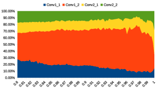
Figure 3: energy distribution comparison of layer “conv1_1”, “conv1_2”, “conv2_1” and “conv2_2”. The horizontal axis represents normalized magnitude from 0.8 to 1, and the area shows the comparison of each layer’s normalized energy.

6 Conclusion

In this paper, we designed a CNN accelerator that substituted floating point representation with BFP representation. Using BFP, the burdensome floating-point arithmetics in convolution layers, which is the majority of the overall CNN architecture, are replaced by the light fixed-point arithmetics. Using 8-bit mantissa, the worst accuracy drop of deep neural networks is less than 0.3% without retraining. In addition, we developed the NSR upper bound analytical model with the largest deviation less than 8.9dB, which provides the guidance for hardware design.

7 Acknowledgement

This work is supported by the National Key Research and Development (2016YFB0200505).

References

- [Chen et al. 2017] Chen, Y.-H.; Krishna, T.; Emer, J. S.; and Sze, V. 2017. Eyeriss: An energy-efficient reconfigurable accelerator for deep convolutional neural networks. IEEE Journal of Solid-State Circuits 52(1):127–138.
- [Chunsheng et al. 2017] Chunsheng, M.; Zhenyu, L.; Yue, N.; Xiangyang, J.; Wei, Z.; and Dongsheng, W. 2017. A 200mhz 202.4gflops@10.8w vgg16 accelerator in xilinx vx690t. In IEEE Global Conference on Signal and Information Processing, accepted. IEEE.
- [Ciregan, Meier, and Schmidhuber 2012] Ciregan, D.; Meier, U.; and Schmidhuber, J. 2012. Multi-column deep neural networks for image classification. In Computer Vision and Pattern Recognition (CVPR), 2012 IEEE Conference on, 3642–3649. IEEE.
- [Glorot, Bordes, and Bengio 2011] Glorot, X.; Bordes, A.; and Bengio, Y. 2011. Deep sparse rectifier neural networks. In Proceedings of the Fourteenth International Conference on Artificial Intelligence and Statistics, 315–323.
- [Goldberg 2016] Goldberg, Y. 2016. A primer on neural network models for natural language processing. J. Artif. Intell. Res.(JAIR) 57:345–420.
- [Gupta et al. 2015] Gupta, S.; Agrawal, A.; Gopalakrishnan, K.; and Narayanan, P. 2015. Deep learning with limited numerical precision. In Proceedings of the 32nd International Conference on Machine Learning (ICML-15), 1737–1746.
- [Han et al. 2015] Han, S.; Pool, J.; Tran, J.; and Dally, W. 2015. Learning both weights and connections for efficient neural network. In Advances in Neural Information Processing Systems, 1135–1143.
- [Han, Mao, and Dally 2015] Han, S.; Mao, H.; and Dally, W. J. 2015. Deep compression: Compressing deep neural networks with pruning, trained quantization and huffman coding. arXiv preprint arXiv:1510.00149.
- [He et al. 2016] He, K.; Zhang, X.; Ren, S.; and Sun, J. 2016. Deep residual learning for image recognition. In Proceedings of the IEEE conference on computer vision and pattern recognition, 770–778.
- [Hill et al. 2016] Hill, P.; Zamirai, B.; Lu, S.; Chao, Y.-W.; Laurenzano, M.; Samadi, M.; Papaefthymiou, M.; Mahlke, S.; Wenisch, T.; Deng, J.; et al. 2016. Rethinking numerical representations for deep neural networks.
- [Jia et al. 2014] Jia, Y.; Shelhamer, E.; Donahue, J.; Karayev, S.; Long, J.; Girshick, R.; Guadarrama, S.; and Darrell, T. 2014. Caffe: Convolutional architecture for fast feature embedding. arXiv preprint arXiv:1408.5093.
- [Jouppi et al. 2017] Jouppi, N. P.; Young, C.; Patil, N.; Patterson, D.; Agrawal, G.; Bajwa, R.; Bates, S.; Bhatia, S.; Boden, N.; Borchers, A.; et al. 2017. In-datacenter performance analysis of a tensor processing unit. arXiv preprint arXiv:1704.04760.
- [Kalliojarvi and Astola 1996] Kalliojarvi, K., and Astola, J. 1996. Roundoff errors in block-floating-point systems. IEEE Transactions on Signal Processing 44(4):783–790.
- [Karam et al. 2017] Karam, R.; Paul, S.; Puri, R.; and Bhunia, S. 2017. Memory-centric reconfigurable accelerator for classification and machine learning applications. ACM Journal on Emerging Technologies in Computing Systems (JETC) 13(3):34.
- [Kim 2014] Kim, Y. 2014. Convolutional neural networks for sentence classification. arXiv preprint arXiv:1408.5882.
- [Li et al. 2016] Li, H.; Fan, X.; Jiao, L.; Cao, W.; Zhou, X.; and Wang, L. 2016. A high performance fpga-based accelerator for large-scale convolutional neural networks. In Field Programmable Logic and Applications (FPL), 2016 26th International Conference on, 1–9. IEEE.
- [Liu et al. 2016] Liu, Z.; Yu, X.; Gao, Y.; Chen, S.; Ji, X.; and Wang, D. 2016. Cu partition mode decision for hevc hardwired intra encoder using convolution neural network. IEEE Transactions on Image Processing 25(11):5088–5103.
- [Mellempudi et al. 2017] Mellempudi, N.; Kundu, A.; Das, D.; Mudigere, D.; and Kaul, B. 2017. Mixed low-precision deep learning inference using dynamic fixed point. arXiv preprint arXiv:1701.08978.
- [Ovtcharov et al. 2015] Ovtcharov, K.; Ruwase, O.; Kim, J.-Y.; Fowers, J.; Strauss, K.; and Chung, E. S. 2015. Accelerating deep convolutional neural networks using specialized hardware. Microsoft Research Whitepaper 2(11).
- [Page and Mohsenin 2016] Page, A., and Mohsenin, T. 2016. Fpga-based reduction techniques for efficient deep neural network deployment. In Field-Programmable Custom Computing Machines (FCCM), 2016 IEEE 24th Annual International Symposium on, 200–200. IEEE.
- [Parashar et al. 2017] Parashar, A.; Rhu, M.; Mukkara, A.; Puglielli, A.; Venkatesan, R.; Khailany, B.; Emer, J.; Keckler, S. W.; and Dally, W. J. 2017. Scnn: An accelerator for compressed-sparse convolutional neural networks. In Proceedings of the 44th Annual International Symposium on Computer Architecture, 27–40. ACM.
- [Russakovsky et al. 2015a] Russakovsky, O.; Deng, J.; Su, H.; Krause, J.; Satheesh, S.; Ma, S.; Huang, Z.; Karpathy, A.; Khosla, A.; Bernstein, M.; Berg, A. C.; and Fei-Fei, L. 2015a. ImageNet Large Scale Visual Recognition Challenge. International Journal of Computer Vision (IJCV) 115(3):211–252.
- [Russakovsky et al. 2015b] Russakovsky, O.; Deng, J.; Su, H.; Krause, J.; Satheesh, S.; Ma, S.; Huang, Z.; Karpathy, A.; Khosla, A.; Bernstein, M.; et al. 2015b. Imagenet large scale visual recognition challenge. International Journal of Computer Vision 115(3):211–252.
- [Silver et al. 2016] Silver, D.; Huang, A.; Maddison, C. J.; Guez, A.; Sifre, L.; Van Den Driessche, G.; Schrittwieser, J.; Antonoglou, I.; Panneershelvam, V.; Lanctot, M.; et al. 2016. Mastering the game of go with deep neural networks and tree search. Nature 529(7587):484–489.
- [Simonyan and Zisserman 2014] Simonyan, K., and Zisserman, A. 2014. Very deep convolutional networks for large-scale image recognition. arXiv preprint arXiv:1409.1556.
- [Szegedy et al. 2015] Szegedy, C.; Liu, W.; Jia, Y.; Sermanet, P.; Reed, S.; Anguelov, D.; Erhan, D.; Vanhoucke, V.; and Rabinovich, A. 2015. Going deeper with convolutions. In The IEEE Conference on Computer Vision and Pattern Recognition (CVPR).
- [Zhang et al. 2015] Zhang, C.; Li, P.; Sun, G.; Guan, Y.; Xiao, B.; and Cong, J. 2015. Optimizing fpga-based accelerator design for deep convolutional neural networks. In Proceedings of the 2015 ACM/SIGDA International Symposium on Field-Programmable Gate Arrays, 161–170. ACM.