Using Markov Models and Statistics to Learn, Extract, Fuse, and Detect Patterns in Raw Data

Abstract

Many systems are partially stochastic in nature. We have derived data-driven approaches for extracting stochastic state machines (Markov models) directly from observed data. This chapter provides an overview of our approach with numerous practical applications. We have used this approach for inferring shipping patterns, exploiting computer system side-channel information, and detecting botnet activities. For contrast, we include a related data-driven statistical inferencing approach that detects and localizes radiation sources.

1 Introduction

Markov models have been widely used for detecting patterns sin1999network ; van2007using ; brooks2009behavior ; bhanu2011side ; lu2012network ; lu2011botnet ; fu2017botnet ; fu2017stealthy . The premise behind a Markov models is that the current state only depends on the previous state and that transition probabilities are stationary. This makes Markov models versatile, as this is a direct result of the causal world we live in. Often, these models can only be partially observed. In that case, we refer to the collective (observable and non-observable) model as a hidden Markov model (HMM).

Stochastic processes can successfully model many system signals. Some of these systems cannot be accurately represented using a Markov model or an HMM due to the uncertainty of input data. One task that benefits from stochastic signal processing is the detection and localization of radioactive sources. Since radioactive decay follows a Poisson distribution Knoll2000 , radiation measurements must be treated as stochastic variables. A prevalent method for localizing radioactive sources is maximum likelihood estimation (MLE) Gunatilaka2007 ; deb2013iterative ; CordoneExpansion2017 , we consider bootstrapping the MLE using estimates from a linear regression model CordoneMLERegression .

In Section 2, background information about Markov models is presented, along with references to our previous work developing the methods presented here. Section 3 discusses new developments in the inference of HMMs, detection using HMMs, methods for determining the significance of HMMs, HMM metric spaces, and applications that use HMM-based detection. Section 4 analyzes radiation processes, maximum likelihood localization, and the use of linear regression to estimate source and background intensities. In Section 5, closing remarks are presented.

2 Background information and previous work

A Markov model is a tuple $G=(S,T,P)$, where $S$ is a set of states, $T$ is a set of directed transitions between the states, and $P=\left\{p(s_{i},s_{j})\right\}$ is a probability matrix associated with transitions from state $s_{i}$ to $s_{j}$ such that:

$$\sum\nolimits_{s_{j}\in S}p(s_{i},s_{j})=1,\quad\forall s_{i}\in S$$ (1)

In a Markov model, the next state depends only on the current state. An HMM is a Markov model with unobservable states. A standard HMM eddy1996hidden ; rabiner1989tutorial has two sets of random processes: one for state transition and the other for symbol outputs. Our model is a deterministic HMM lu2013normalized ; lu2012network ; schwier2009pattern , which only has one random process for state transitions. Therefore, given the current state and the symbol associated with the outgoing transition, the next state is deterministic. For each deterministic HMM there is an equivalent standard HMM and vice versa vanluyten2008equivalence . This deterministic property helps us infer HMMs from observations.

Schwier et al. schwier2011methods developed a method for determining the optimal window size to use when inferring a Markov model from serialized data. Brooks et al. brooks2009behavior found that HMM confidence intervals performed better than the maximum likelihood estimate. This was illustrated through an analysis of consumer behavior. Building on this work, Lu et al. yu2013inferring devised a method for determining the statistical significance of a model, as well as determining the number of samples required to obtain a model with a desired level of statistical significance.

3 Markov modeling

3.1 Infering hidden Markov models

HMM inference discovers the HMM structure and state transition probabilities from a sequence of output observations. Traditionally, the Baum-Welch algorithm rabiner1989tutorial is used to infer the state transition matrix of a Markov chain and symbol output probabilities associated with the states of the chain, given an initial model and a sequence of symbols. As a result, this algorithm requires the a priori structural knowledge of the Markov process that produced the outputs.

Schwier et. al schwier2009zero developed the zero-knowledge HMM inference algorithm. The assumption of HMM inference is (1) the transition probabilities are constant; (2) the distribution of the underlying HMM is the stationary; and (3) the Markov process is ergodic. In essence, this means that the system is Markovian, non-periodic and has a single strongly connected component. The input of the algorithm is a string of symbols, and the output is the HMM. If the input data are not provided as a set of strings, but rather as a set of continuous trajectories, then  griffin2011hybrid explains how to change trajectories into symbolic strings.

The original algorithm only requires one parameter, $L$, as the input, which refers to the maximum number of history symbols used to infer the HMM state space and estimate associated probabilities. Take ‘abc’ as an example input string. For $L=1$, it calculates transition probabilities $P(a|a)$, $P(a|b)$, $P(a|c)$, and so on, by creating a state for each symbol and counting how many times the substrings ‘aa’, ‘ab’, and ‘ac’ occur in the training data and dividing them by the number of occurences of the symbol ‘a’. The chi-squared test is used to compare the outgoing probability distributions for all pairs of states. If two states are equivalent, they are merged.

For $L=2$, the number of states used for representing conditional probabilities is squared. For example, in a system that has $L=2$, it could be the case that $P(c|a)\neq P(c|aa)$. In which case ‘a’ and ‘aa’ will be different states. The state space increases exponentially with $L$, as does the time needed to infer the HMM. We showed that $L$ can be determined automatically as part of HMM inference. The idea is to keep increasing $L$ until the HMM model stabilizes, i.e. $HMM(L)==HMM(L+1)$. This data-driven approach finds the system HMM with no a priori information. Tis process is decribed in detail in schwier2009zero ; schwier2009pattern .

If an insufficient amount of observation data is used to generate the HMM, the model will not be representative of the actual underlying process. A model confidence test is used to determine if the observation data and constructed model fully express the underlying process with a given level of statistical significance yu2013inferring . This approach calculates an lower bound on the number of samples required. If the number of input samples is less than the bound, more data is required. New models should be inferred with more data and still need to be checked for confidence. This approach allows us to remove the effect of noise in the HMM inference.

3.2 Detection with HMM

Once the HMM is inferred from symbolized data and passes the model confidence test, it can be used to detect whether or not a data sequence was generated by the same process. The traditional Viterbi Algorithm rabiner1989tutorial finds the HMM that was most likely to generate the data sequence by comparing probabilities generated by the HMMs. For data streams, it is unclear what sample size to use with the Viterbi algorithm. Also as data volume increases, the probability produced by the Viterbi algorithm decreases exponentially, and may suffer floating point underflow brooks2009behavior . To remedy this, confidence intervals (CIs) are used brooks2009behavior . With this approach, the certainty of detection increases with the number of samples and the floating point underflow issues of the Viterbi Algorithm is eliminated brooks2009behavior . The CI approach can determine, for example, whether or not observed network traffic was generated by a botnet HMM.

Given a sequence of symbolized traffic data and a HMM, the CI method in brooks2009behavior traces the data through the HMM and estimates the transition probabilities and confidence intervals. This process maps the observation data into the HMM structure. It then determines the proportion of original transition probabilities that fall into their respective estimated CIs. If this percentage is greater than a threshold value, it accepts that the traffic data adequately matches the HMM.

Lu et al. lu2012network used an alternative approach. Instead of estimating transition probabilities and corresponding CIs, they calculated the state probabilities, which are the proportion of time the system stays in a specific state, and their corresponding CIs. Once all state probabilities and CIs were estimated for the observation sequence, they determined whether each state is within a certain confidence interval. For the whole HMM, the proportion of states was obtained whose estimated state probability matched the corresponding confidence intervals. If an observation sequence was generated from the HMM, it would follow the state transitions of the underlying stochastic process that the HMM represents, and its state probabilities would converge to the asymptotic state probabilities if the sequence length was large enough. Therefore, more states would match their estimated CIs. Generally, a sequence that is generated by the HMM would have a high proportion of matching probabilities, while a sequence that is not an occurrence of the HMM will have a low proportion of matching probabilities. Similar to the detection approach in brooks2009behavior , a threshold value can be set for this proportion of matching states, to determine whether the observation sequence matches with the HMM.

In brooks2009behavior , receiver operating characteristic (ROC) curves were used to find optimal threshold values. By varying the threshold from 0% to 100% (0% threshold means we accept everything and we will have a high false positive rate. 100% threshold means we reject everything and we will have a low true positive rate), they progressively increased the criteria for acceptance. Using the ROC curve drawn from detection statistics with different thresholds, the closest point to (0,1) was found, which represents 0% false positive rate and 100% true positive rate. This considered the trade-off between true positive and false positive rates. Therefore, the corresponding threshold of that point was the optimal threshold value.

3.3 Statistically significant HMMs

In yu2013inferring , we address the problem of how to ensure the inferred HMM accurately represents the underlying process that generates the observation data. The measure of the accuracy is known as model confidence, which means the degree to which a model represents the underlying process that generated the training data. As illustrated in Figure 1, model confidence is different from model fidelity, where the latter refers to the agreement between the inferred model and the training data.

Figure 1: Hierarchy of the process, observations, and model showing the relationship between model fidelity and model confidence (adopted from yu2013inferring ).

Mathematically, we calculate an upper bound on the number of samples required to guarantee that the constructed model has a given level significance. In other words, we have shown how to determine within a given level of statistical confidence ($\alpha$) if a “known unknown” transition does not occur, given two user-defined thresholds $\epsilon$ and $\alpha$. The parameter $\epsilon$ determines the minimum probability that transitions with probabilities no less than $\epsilon$ should be included in the constructed model. The parameter $\alpha$ is the confidence level that shows the accuracy of the model result.

For each state, $s$, we use the $z$-test bowerman1990linear to determine if the inferred model includes all transitions with probabilities no smaller than $\gamma_{s}^{\epsilon}={\epsilon}/{\pi_{s}}$ with desired significance $\alpha$, where $\pi_{s}$ is the asymptotic probability of $s$ as the constructed Markov model is irreducible. Concretely, we test the null hypothesis $H_{0}$: $\overline{X_{s}^{U}}=\gamma_{s}^{\epsilon}$ against the alternative hypothesis $H_{1}$: $\overline{X_{s}^{U}}<\gamma_{s}^{\epsilon}$, where $\overline{X_{s}^{U}}$ denote the sample average of the probability of an unobserved transaction of state $s$. We use $\gamma_{s}^{\epsilon}-\overline{X_{s}^{U}}$ as a test statistic, rejecting the null hypothesis if $\gamma_{s}^{\epsilon}-\overline{X_{s}^{U}}$ is too large. We have not observed the transition, thereby $\overline{X_{s}^{U}}=0$. We fail to reject $H_{0}$ if we need to collect more data. Otherwise, we say that sufficient data has been collected. If we fail to reject the null hypothesis for all states, the $z$-test also finds the minimum amount of training samples needed for transaction transitions with probabilities no smaller than $\gamma_{s}^{\epsilon}$ to be detected with desired level of significance $\alpha$.

To use the $z$-test in this manner, we propose a simple algorithm to perform on-line testing of the observation sequence. The algorithm determines if a constructed model statistically represents a data stream in the process of being collected. We first collect a sequence of observation data $\mathbf{y}$ of some length $D$ and construct a model from the collected data. With the constructed model, we determine the $z$-statistics and find if the experimental statistic provides $100\cdot(1-\alpha)\%$ confidence that a transition with probability $\epsilon$ does not occur. If $\mathbf{y}$ is not sufficiently long, we will be unable to construct a model from the data; additional data should be gathered. The algorithm is provided in yu2013inferring .

3.4 HMM metric space

A metric is a mathematical construct that describes the similarity (or difference) between two models. It is useful to know if two processes are the same, except for rare events (e.g., events occurring once in a century), since we would typically consider them functionally equivalent. Eliminating duplicate models can reduce system complexity by decreasing the number of models used to analyze using observation data. Grouping similar models can increase the number of samples available for model inference, leading to higher fidelity system representations.

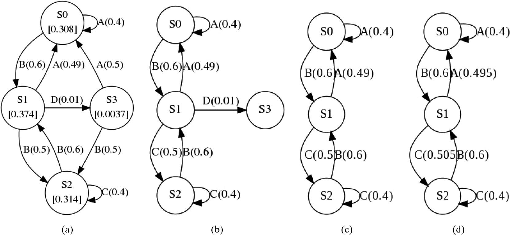
Figure 2: Process to remove transitions: (a) original model (asymptotic state probabilities are in square brackets); (b) initial step with $P_{th}=0.002$; (c) removal of absorbing states; and (d) resulting model with rescaled probabilities. (adopted from lu2013normalized ).

To determine if two deterministic HMMs $G_{1}$ and $G_{2}$ are equivalent, we first let $G_{1}$ generate an observation sequence $\mathbf{y}$ of length $D$ and then run $\mathbf{y}$ through $G_{2}$. Using frequency counting, we obtain a set of sample transition probabilities for each transition of $G_{2}$, denoted by $T^{\prime}_{2}$. The probabilities of all outgoing transitions conditioning on each state follow multinomial distribution, which are then approximated by a set of binomial distributions in this context. This allows us to use the standard $\chi^{2}$-test to compare if the two sets of transition distributions $\{T^{\prime}_{2},T_{2}\}$ are equivalent with significance $\alpha$ kutner2004applied , where $T_{2}$ is the set of transitions probabilities of $G_{2}$. We define equivalence $(G_{1}\equiv G_{2})$ as $G_{1}$ and $G_{2}$ accepting the same symbol sequences with a user-defined statistical significance $\alpha$. The corresponding algorithm is provided in lu2013normalized . Note that, if there does not exist a path across $G_{2}$ that yields observation sequence $\mathbf{y}$, we can immediately conclude that $G_{1}$ and $G_{2}$ are not equivalent.

If $G_{1}$ and $G_{2}$ are not equivalent, we quantify the distance between them as how much their statistics differ with significance $\alpha$. Given a probability $0\leq P_{th}\leq 1$, we prune all transactions with probability no greater than $P_{th}$ from both models and then re-normalize the probabilities of remaining transitions for each state to obtain two sub-models. The pruning process is illustrated in Figure 2 using a simple model with threshold value $P_{th}=0.002$. The distance between the two models is defined as the minimum $P_{th}$ that yields two equivalent sub-models. To determine this distance, we progressively remove the least likely events from both models until the remaining sub-models are considered equivalent. Specifically, starting from $P_{th}=0$, we prune all transactions with probability no greater than $P_{th}$, and then re-normalize the probabilities of remaining transactions for each state. We gradually increase $P_{th}$ and repeat the pruning operation for each $P_{th}$ until the remaining sub-models are considered equivalent with the predefined confidence level $\alpha$. Let $d(G_{1},G_{2})$ denote the statistical distance between $G_{1}$ and $G_{2}$, then $d(G_{1},G_{2})$ is equal to the stopping value of $P_{th}$. We show in lu2013normalized that $d(G_{1},G_{2})$ is a metric as it fulfills all the necessary conditions as a metric.

Since the $\chi^{2}$-test is used, we need to ensure that enough samples ($D$) are used for transition probabilities to adequately approximate normal distributions. In order to approximate the binomial distribution as normal distribution, the central limit theorem is used to calculate the required sample size.

This is similar in spirit to Kullback–Leibler divergence (KLD); however, unlike KLD, our approach is a true metric. It does not have KLD’s limitations and provides a statistical confidence value for the distance. We illustrated the performance of the metric by calculating the distance between different, similar, and equivalent models. Compared with KLD measurement, our approach is more practical and provides a true metric space.

3.5 HMM detection applications

We have used this approach to:

Track shipping patterns in the North Atlantic;

Identify protocol use within encrypted VPN traffic;

Identify the language being typed in an SSH session;

Identify botnet traffic;

Identify smart grid traffic within encrypted tunnels and disrupt data transmission;

Create transducers that transform the syntax of one network protocol into another one; and

De-anonymize bitcoin currency transfers.

Track shipping patterns in the North Atlantic

Symbolic Transfer Functions (STF) were developed for modeling stochastic input/output systems whose inputs and outputs are both purely symbolic. Griffin et al. griffin2011hybrid applied STFs to track shipping patterns in the North Atlantic by assuming the input symbols represent regions of space through which a track is passing, while the output represents specific linear functions that more precisely model the behavior of the track. A target’s behavior is modeled at two levels of precision: the symbolic model provides a probability distribution on the next region of space and behavior (linear function) that a vehicle will execute, while the continuous model predicts the position of the vehicle using classical statistical methods. They collected over 8 months worth of data for 13 distinct ships, representative of a variety of vessel classes (including cruise ships, Great Lakes trading vessels, and private craft). The STF algorithm was used to produce a collection of vessel track models. The models were tested for their prediction power over the course of three days.

Identify protocol use within encrypted VPN traffic

A VPN is an encrypted connection established between two private networks through the public network. Packets transferred through a VPN tunnel have the source and destination IP of the private networks, which are not always the final destination of the packet. The destination IPs for each packet are encrypted and cannot be seen by any third party. A typical VPN implementation encrypts the packets with little overhead and pads all packets in a given size range to the same size. Thus, the timing side-channel and packet size side-channel can be used to identify the underlying protocol even after encryption. These side-channels are shown in Figure 3. In zhong2015twoPMU , a synchrophasor network protocol is identified in an encrypted VPN tunnel.

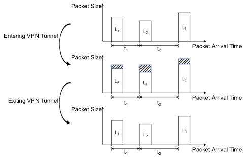
Figure 3: Timing and size side-channels in a VPN tunnel.

Identify the language being typed in an SSH session

SSH encryption is mathematically difficult to break, but the implementation is vulnerable to side-channel analysis. In an interactive SSH session, users’ keystroke-timing data are associated with inter-packet delays. In harakrishnan2011side , the inter-packet delays are used to determine the language used by the victim. This is achieved by comparing the observed data with the HMM of known languages. In Song:2001:TAK:1251327.1251352 , the timing side-channel is used to extract the system password from interactive SSH sessions.

Identify botnet traffic

Botnets are becoming a major source of spam, distributed denial-of-service attacks (DDoS), and other cybercrime. Chen et al lu2011botnet used traffic timing information to detect the centralized Zeus botnet. The reasons to use timing information are: (1) inter-packet timings relate to the command and control processing time of the botnet; (2) the bots periodically communicate with the command and control (C&C) server for new commands or new data; (3) the inter-packet delays filter out constant communication latencies; and (4) it does not require reverse engineering the malware binaries or encrypted traffic data. An HMM is inferred from inter-packet delays of Zeus botnet C&C communication traffic. Using the behavior detection method with confidence intervals (CIs) of HMMs brooks2009behavior , they were able to detect whether or not a sequence of traffic data is botnet traffic. Experimental results showed this approach can properly distinguish wild botnet traffic from normal traffic.

Identify smart grid traffic within encrypted tunnels and disrupt data transmission

In a power grid, Phasor Measurement Units (PMU) send measurement data (or synchrophasor data) over the Internet to a control center for closed loop control. Any unexpected change in the variance of the packet delay can cause instability in the power grid and even blackouts. PMUs are deployed at critical locations and are usually protected by security gateways.

The use of security gateways and VPN tunnels to encrypt PMU traffic eliminates many possible vulnerabilities beasley2014survey ; zhong2015cyber , but these devices are still vulnerable to Denial of Service (DoS) attacks that exploit a side-channel vulnerability. In zhong2017ETCI , encrypted PMU measurement traffic is identified and dropped through an exploitation of side-channel vulnerabilities. The underlying protocol is detected as described in Section 3.5, and the target protocol’s packets are dropped. The attack leads to unstable power grid operations. Figure 4 illustrates such an attack. This attack is tough to detect because only the measurement traffic is dropped, and all other traffic is untouched (e.g. ping or SSH traffic). From the victim’s point of view, all systems works fine, but no measurement traffic is received.

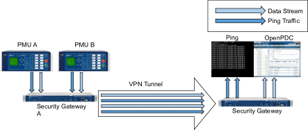
(a)

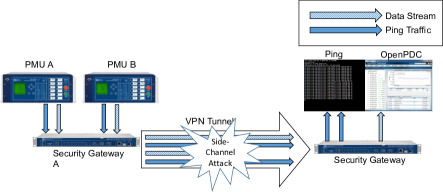
(b)

Figure 4: An example of a DoS attack in a VPN tunnel: (a) A VPN network carries Ping traffic and data streams from two PMUs to control center; (b) During a DoS attack, a PMU data stream within the VPN tunnel is identified and dropped.

Botnet Domain Generation Algorithm (DGA) modeling and detection

Botnets have been problematic for over a decade. In response to take-down campaigns, botmasters have developed techniques to evade detection. One widely used evasion technique is DNS domain fluxing. Domain names generated with Domain Generation Algorithms (DGAs) are used as the rendezvous points between botmasters and bots. In this way, botmasters hide the real location of the C&C servers by changing the mapping between IP addresses and domain names frequently. Fu et al. fu2017stealthy developed a new DGA using HMMs, which can evade current DGA detection methods (Kullback-Leibler distance, Edit distance, and Jaccard Index)yadav2010detecting and systems (Botdigger zhang2016botdigger and Pleiades antonakakis2012throw ). The idea is to infer an HMM from the entire space of IPv4 domain names. Domain names generated by the HMM are guaranteed to have the same lexical features as the legitimate domain names. With the opposite idea, two HMM-based DGA detection methods were proposed fu2017botnet . Since the HMM expresses the statistical features of the legitimate domain names, the corresponding Viterbi path of a given domain name can be found, which indicates the likelihood that the domain name is generated by the HMM. The probability returned by the HMM is a measure of how consistent the domain name is with the set of legitimate domain names.

A covert data transport protocol

Protocol obfuscation is widely used for evading censorship and surveillance and hiding criminal activity. Most firewalls use DPI to analyze network packets and filter out sensitive information. However, if the source protocol is obfuscated or transformed into a different protocol, detection techniques won’t work zhong2015stealthy . Fu et al. fu2016covert developed a covert data transport protocol that transforms arbitrary network traffic into legitimate DNS traffic in a server-client communication model. The server encodes the message into a list of domain names and register them to a randomly chosen IP address. The idea of the encoding is to find a unique path in the HMM inferred from legitimate domain names, which is associated with the message. The client does a reverse-DNS lookup on the IP address and decodes the domain names to retrieve the message. Compared to DNS tunneling, this method doesn’t use uncommon record types (TXT records) or carry suspiciously large volume of traffic as DNS payloads. On the contrary, the resulting traffic will be normal DNS lookup/reverse-lookup traffic, which will not attract attention. The data transmission is not vulnerable to DPI.

Bitcoin Transaction Analysis

Bitcoin has been the most successful digital currency to date. One of the main factors contributing to Bitcoin’s success is the role it has found in criminal activity. According to Christin christin2013traveling , in 2012 the Silk Road (a popular dark web marketplace) was handling 1.2 million USD worth of Bitcoin transactions each month. This is largely attributed to Bitcoin’s appeal–pseudonymity, which disassociates users with the publicly available transactions.

Figure 5: An example of a Bitcoin transaction found in the public blockchain.

It is natural to consider financial transactions as a Markovian process since each transaction is governed solely by previous states. All Bitcoin transactions can be publicly viewed on the blockchain, as shown in Figure 5. This motivates the notion that transactions can be represented by a Markov model. However, since Bitcoin is pseudonymous, there are hidden states that correspond to the Bitcoin users. The process of grouping the observable transactions with their respective users infers the underlying HMM.

Theoretically, this HMM would render traditional Bitcoin money laundering useless since existing Bitcoin laundering techniques are reminiscent of a shell game. Current research is focused on inferring the HMM from the Bitcoin blockchain, leveraging existing research that identifies transient transactions used for change functionality barber2012bitter ; ober2013structure .

4 Stochastic Signal Processing for Radiation Detection and Localization

4.1 Radiation Processes

The detection and localization of radioactive sources, especially those that emit ionizing gamma radiation, is a problem that is of great interest for national security uscongress2010 . Such a task is not simple due to the physics of radiation signal propagation, the stochastic nature of radiation measurements, and interference from background noise. Assuming a uniform propagation medium between the source and location of measurement, as well as a negligible attenuation due to the medium, a simple radiation propagation model is given by

$$I=\frac{A}{x^{2}}+B,$$ (2)

where $I$ is the total radiation intensity at the measurement location, $A$ is the intensity of the radioactive source, $x$ is the distance from the source to the measurement location, and $B$ is the intensity of the background radiation at the measurement location.

It is evident from (2) that propagation of the signal from a radioactive point source is governed by the inverse-square law, which states that the intensity of the signal is inversely proportional to the distance from the source. Figure 6 provides a visual example of the effect the inverse-square law has on the intensity of a radiation signal.

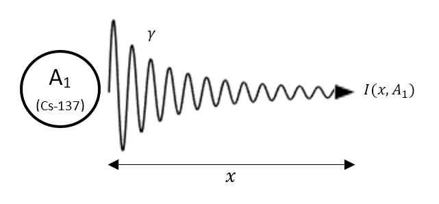
Figure 6: The intensity of a radiation signal decreases exponentially with distance when moving through a uniform medium

Ionizing radiation is commonly measured using scintillation counters, which integrate the number of times that an incident gamma particle illuminates a scintillation material over a given time period. The number of incidents integrated over each time period are referred to as ‘counts.’ Due to the physics of radioactive decay, the measurements of scintillation counters are Poisson random variables Knoll2000 . As a result, single radiation measurements are unreliable since the measurement of a high intensity source will have a proportionally high variance. An example of the difference in variance between a high intensity and low intensity signal is given in Figure 7. Observe that the high intensity signal recorded one meter from the source has a much higher range of values than the low intensity signal recorded six meters from the source.

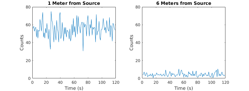
Figure 7: Real measurements of a 35 $\mu Ci$ Cs-137 source at various distances (IRSS datasets irss )

4.2 Maximum Likelihood Estimation

Basic radiation detection methods for national security involve the deployment of one or two sensors in the form of portal monitors located at choke points along the road. While simple and reliable for detection, the use of portal monitors is not practical for several locations, such as a widespread urban environment with complex road networks Brennan2004 . Recently, the major focus of research has been on the use of distributed networks of detectors, which are much more suitable for the detection and localization of radiation sources over a widespread area. With a distributed detector network, the detection and localization of radiation sources becomes a complex problem requiring the fusion of large amounts of stochastic data. One of the most common fusion methods used for this purpose is Maximum Likelihood Estimation Gunatilaka2007 ; chin2008 ; vilim2009radtrac .

In short, Maximum Likelihood Estimation (MLE) is a search over all possible parameters of the target radiation source. While the number of parameters depends on the radiation model, they commonly include the horizontal and vertical coordinates of the source and the radioactive intensity of the source. Each combination of possible parameters are plugged into a likelihood function, which gives the probability that a source with the given parameters cause each detector in the field to have their current measurements. The parameters that generate the highest likelihood are selected as the maximum likelihood estimate of the source. An example likelihood function based on the radiation model in (2) is given by

$$L(\theta)=\sum_{i=1}^{N_{d}}\left(\ln{I_{i}}\sum_{j=1}^{w}\left(c_{ij}-1\right)\right),$$ (3)

where $N_{d}$ is the number of detectors being used for the localization, $w$ is the length of the time window, $c_{ij}$ is the measurement for the $i$th detector at timestep $j$, and $\theta$ is the vector of input source parameters, which are used to generate the the intensity at the $i$th detector, $I_{i}$, using (2). The maximization of the likelihood function is then given as

$$\hat{\theta}_{ml}=\arg{\max{L(\theta)}},$$ (4)

where $\hat{\theta}_{ml}$ is the maximum likelihood estimate of the source parameter vector. A visual example of an MLE localization is shown in Figure 8. Note that the likelihood function in (3) is a simplification of the logarithm of the joint Poisson probability for the likelihood of the measurements at each individual detector CordoneExpansion2017 .

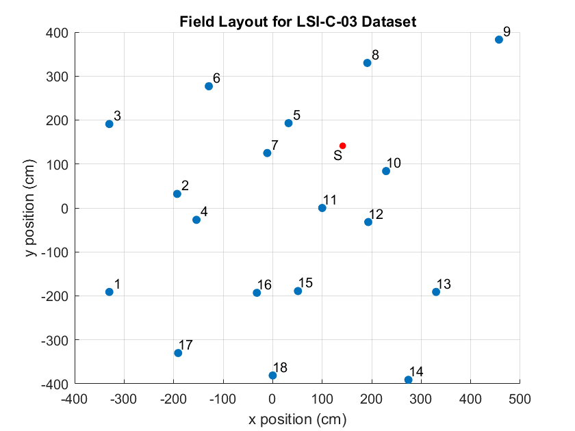
(a)

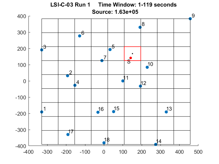
(b)

Figure 8: An example of a low resolution MLE localization: (a) Layout of a detector field from IRSS datasets irss . Detectors are blue dots indexed by numbers and the radiation source is a red dot tagged with an ’S’. (b) A coarse MLE localization has been performed over the detector field. The center of each grid region was used as input parameters for (4). The grid region with a red border and a black dot at the center is the area selected by the search.

The primary criticism of MLE localization is that it is computationally intensive, requiring a brute force search over all parameters. A common method for reducing the total computational load of the MLE search is the use of an iterative search deb2013iterative  chin2008 , which allows the large ranges of parameter space to be excluded from the overall localization. While iterative MLE localization is much faster than standard MLE search, throwing out large areas of parameter space makes the search liable to be caught within local maxima Sheng2005 . In CordoneExpansion2017 , we proposed the use of Grid Expansion to mitigate these types of errors. With Grid Expansion, the search area is expanded by a given percent between each iteration, allowing the MLE search to span into areas that would have been thrown out by a standard iterative algorithm. We found that despite a requiring small increase in computation time, the use of Grid Expansion corrected errors in the situations where the search was getting caught within local maxima, while maintaining good localization performance in cases where the error was not occurring.

4.3 Linear Regression

Observe that the radiation propagation model given in (2) is linear with respect to $1/x^{2}$. Furthermore, by the law of large numbers, the average of the Poisson distributed detector measurements over a large time window are representative of the radiation intensity at their respective locations. Given these two observations, a linear regression model built using the average detector measurements over a large enough time window and their distances to the source location may be used to estimate both the source and background intensities, where the slope of the regression line is the source intensity estimate and the intercept of the regression line is the background intensity estimate. Figure 9 shows a linear regression model built using detector data and their inverse-squared distances to a source location estimate over a ten second time window. In CordoneNSS2017 , we use the source estimate from a linear regression model to successfully detect the presence of a moving source within a distributed detector field.

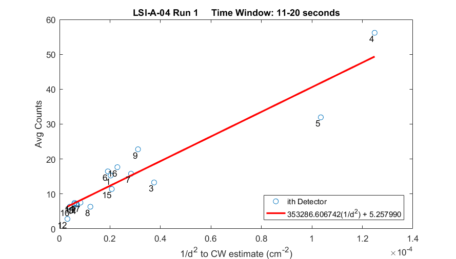
Figure 9: A linear regression model built on average detector measurements vs. their inverse squared distance to an estimate of the source location. The source and background intensity estimates are provided by the slope and intercept values of the line, which are around $3.533\times 10^{5}$ counts and 5.258 counts, respectively.

Linear Regression and MLE

One of the difficulties of Maximum Likelihood Estimation is the initialization of the search over state space. In a real time scenario, it is ideal to use small search ranges as a means to conserve computational power and keep the localization up to date with the influx of detector data. While the search area for the position parameters is typically well defined, the search range over the source intensity parameter is not nearly as obvious and can span a large range of possible values. Furthermore, an MLE localization requires prior knowledge of the background intensity, $B$, since computation of the likelihood function (3) requires the solution of the propagation model (2). In CordoneMLERegression , we show that the source intensity and background estimates provided by the linear regression model can be used to speed up an MLE localization by reducing the search range over the intensity parameter and allowing the removal of detectors from the localization whose measurements are most likely to only include background noise.

5 Conclusions

In this chapter we highlighted the use of Markov models and stochastic signal processing to learn, extract, fuse, and detect patterns in raw data. In Section 3, we introduced the deterministic Hidden Markov Model (HMM), which is a useful tool to draw information out of a large amount of data. We described the properties of HMM’s and highlighted the usefulness of HMM’s for several detection applications. In Section 4, we described the uses of stochastic signal processing for the detection and localization of radiation sources. We highlighted the advantages and drawbacks of localization with Maximum Likelihood Estimation (MLE) and described the estimation of source and background intensities using a linear regression model based on detector counts.

References

- (1) Antonakakis, M., Perdisci, R., Nadji, Y., Vasiloglou, N., Abu-Nimeh, S., Lee, W., Dagon, D.: From throw-away traffic to bots: Detecting the rise of dga-based malware. In: USENIX security symposium, vol. 12 (2012)
- (2) Barber, S., Boyen, X., Shi, E., Uzun, E.: Bitter to better—how to make bitcoin a better currency. In: International Conference on Financial Cryptography and Data Security, pp. 399–414. Springer (2012)
- (3) Beasley, C., Zhong, X., Deng, J., Brooks, R., Kumar Venayagamoorthy, G.: A Survey of Electric Power Synchrophasor Network Cyber Security. In: Innovative Smart Grid Technologies Conference Europe (ISGT-Europe), 2014 IEEE PES, pp. 1–5 (2014). DOI 10.1109/ISGTEurope.2014.7028738
- (4) Bhanu, H., Schwier, J., Craven, R., Brooks, R.R., Hempstalk, K., Gunetti, D., Griffin, C.: Side-channel analysis for detecting protocol tunneling. Advances in Internet of Things 1(02), 13 (2011)
- (5) Bowerman, B.L., O’connell, R.T.: Linear statistical models: An applied approach. Brooks/Cole (1990)
- (6) Brennan, S.M., Mielke, A.M., Torney, D.C., Maccabe, A.B.: Radiation detection with distributed sensor networks. Computer 37(8), 57–59 (2004). DOI 10.1109/MC.2004.103
- (7) Brooks, R.R., Schwier, J.M., Griffin, C.: Behavior detection using confidence intervals of hidden markov models. IEEE Transactions on Systems, Man, and Cybernetics, Part B (Cybernetics) 39(6), 1484–1492 (2009)
- (8) Chin, J.C., Yau, D.K., Rao, N.S., Yang, Y., Ma, C.Y., Shankar, M.: Accurate localization of low-level radioactive source under noise and measurement errors. In: Proceedings of the 6th ACM conference on Embedded network sensor systems, pp. 183–196. ACM (2008)
- (9) Christin, N.: Traveling the silk road: A measurement analysis of a large anonymous online marketplace. In: Proceedings of the 22nd international conference on World Wide Web, pp. 213–224. ACM (2013)
- (10) Cordone, G., Brooks, R.R., Sen, S., Rao, N.S., Wu, C.Q.: Linear regression for the initialization of radioactive source localization via maximum likelihood estimation Under review
- (11) Cordone, G., Brooks, R.R., Sen, S., Rao, N.S., Wu, C.Q., Berry, M.L., Grieme, K.M.: Improved Multi-Resolution Method for MLE-based Localization of Radiation Sources. Proceedings of the 20th International Conference on Information Fusion, FUSION 2017 (2017)
- (12) Cordone, G., Brooks, R.R., Sen, S., Rao, N.S., Wu, C.Q., Berry, M.L., Grieme, K.M.: Linear regression for radioactive source detection (2017). Accepted for presentation at NSS/MIC 2017
- (13) Deb, B.: Iterative estimation of location and trajectory of radioactive sources with a networked system of detectors. Nuclear Science, IEEE Transactions on 60(2), 1315–1326 (2013)
- (14) Eddy, S.R.: Hidden markov models. Current opinion in structural biology 6(3), 361–365 (1996)
- (15) Fu, Y.: Using botnet technologies to counteract netowrk traffic analysis. Ph.D. thesis, Clemson University (2017)
- (16) Fu, Y., Jiay, Z., Yu, L., Zhong, X., Brooks, R.: A covert data transport protocol. In: Malicious and Unwanted Software (MALWARE), 2016 11th International Conference on, pp. 1–8. IEEE (2016)
- (17) Fu, Y., Yu, L., Hambolu, O., Ozcelik, I., Husain, B., Sun, J., Sapra, K., Du, D., Beasley, C.T., Brooks, R.R.: Stealthy domain generation algorithms. IEEE Transactions on Information Forensics and Security 12(6), 1430–1443 (2017)
- (18) Griffin, C., Brooks, R.R., Schwier, J.: A hybrid statistical technique for modeling recurrent tracks in a compact set. IEEE Transactions on Automatic Control 56(8), 1926–1931 (2011)
- (19) Gunatilaka, A., Ristic, B., Gailis, R.: On localisation of a radiological point source. In: Information, Decision and Control, 2007. IDC’07, pp. 236–241. IEEE (2007)
- (20) Harakrishnan, B., Jason, S., Ryan, C., Richard R, B., Kathryn, H., Daniele, G., Christopher, G.: Side-Channel Analysis for Detecting Protocol Tunneling. Advances in Internet of Things 1(2), 13–26 (2011). DOI 10.4236/ait.2011.12003
- (21) of Homeland Security, U.S.D.: Intelligent radiation sensing system. URL https://www.dhs.gov/intelligent-radiation-sensing-system
- (22) Knoll, G.F.: Radiation Detection and Measurement. John Wiley (2000)
- (23) Kutner, M.H., Nachtsheim, C., Neter, J.: Applied linear regression models. McGraw-Hill/Irwin (2004)
- (24) Lu, C.: Network traffic analysis using stochastic grammars. Ph.D. thesis, Clemson University (2012)
- (25) Lu, C., Brooks, R.: Botnet traffic detection using hidden markov models. In: Proceedings of the Seventh Annual Workshop on Cyber Security and Information Intelligence Research, p. 31. ACM (2011)
- (26) Lu, C., Schwier, J.M., Craven, R.M., Yu, L., Brooks, R.R., Griffin, C.: A normalized statistical metric space for hidden markov models. IEEE transactions on cybernetics 43(3), 806–819 (2013)
- (27) Ober, M., Katzenbeisser, S., Hamacher, K.: Structure and anonymity of the bitcoin transaction graph. Future internet 5(2), 237–250 (2013)
- (28) Rabiner, L.R.: A tutorial on hidden markov models and selected applications in speech recognition. Proceedings of the IEEE 77(2), 257–286 (1989)
- (29) Schwier, J.: Pattern recognition for command and control data systems (2009)
- (30) Schwier, J.M., Brooks, R.R., Griffin, C.: Methods to window data to differentiate between markov models. IEEE Transactions on Systems, Man, and Cybernetics, Part B (Cybernetics) 41(3), 650–663 (2011)
- (31) Schwier, J.M., Brooks, R.R., Griffin, C., Bukkapatnam, S.: Zero knowledge hidden markov model inference. Pattern Recognition Letters 30(14), 1273–1280 (2009)
- (32) Sheng, X., Hu, Y.h.: Maximum Likelihood Multiple-Source Localization Using Acoustic Energy Measurements with Wireless 53(1), 44–53 (2005)
- (33) Sin, B.K., Ha, J.Y., Oh, S.C., Kim, J.H.: Network-based approach to online cursive script recognition. IEEE Transactions on Systems, Man, and Cybernetics, Part B (Cybernetics) 29(2), 321–328 (1999)
- (34) Song, D.X., Wagner, D., Tian, X.: Timing analysis of keystrokes and timing attacks on ssh. In: Proceedings of the 10th Conference on USENIX Security Symposium - Volume 10, SSYM’01. USENIX Association, Berkeley, CA, USA (2001). URL http://dl.acm.org/citation.cfm?id=1251327.1251352
- (35) U.S. Government Publishing Office: Nuclear terrorism: Strengthening our domestic defenses. Senate Hearing 111-1096, Hearings before the Committee on Homeland Security and Governmental Affairs U.S. Senate, 111th Congress, 2nd Session (2010)
- (36) Van, B.L., Garcia-Salicetti, S., Dorizzi, B.: On using the viterbi path along with hmm likelihood information for online signature verification. IEEE Transactions on Systems, Man, and Cybernetics, Part B (Cybernetics) 37(5), 1237–1247 (2007)
- (37) Vanluyten, B., Willems, J.C., De Moor, B.: Equivalence of state representations for hidden markov models. Systems & Control Letters 57(5), 410–419 (2008)
- (38) Vilim, R., Klann, R.: Radtrac: A system for detecting, localizing, and tracking radioactive sources in real time. Nuclear technology 168(1), 61–73 (2009)
- (39) Yadav, S., Reddy, A.K.K., Reddy, A., Ranjan, S.: Detecting algorithmically generated malicious domain names. In: Proceedings of the 10th ACM SIGCOMM conference on Internet measurement, pp. 48–61. ACM (2010)
- (40) Yu, L., Schwier, J.M., Craven, R.M., Brooks, R.R., Griffin, C.: Inferring statistically significant hidden markov models. IEEE Transactions on Knowledge and Data Engineering 25(7), 1548–1558 (2013)
- (41) Zhang, H., Gharaibeh, M., Thanasoulas, S., Papadopoulos, C.: Botdigger: Detecting dga bots in a single network. In: Proceedings of the IEEE International Workshop on Traffic Monitoring and Analaysis (2016)
- (42) Zhong, X., Arunagirinathan, P., Ahmadi, A., Brooks, R., Venayagamoorthy, G.K., Yu, L., Fu, Y.: Side Channel Analysis of Multiple PMU Data in Electric Power Systems. In: Power System Conference (PSC), 2015 Clemson University, pp. 1–6 (2015)
- (43) Zhong, X., Fu, Y., Yu, L., Brooks, R., Venayagamoorthy, G.K.: Stealthy malware traffic-not as innocent as it looks. In: Malicious and Unwanted Software (MALWARE), 2015 10th International Conference on, pp. 110–116. IEEE (2015)
- (44) Zhong, X., Jayawardene, I., Venayagamoorthy, G.K., Brooks, R.R.: Denial of service attack on tie-line bias control in a power system with pv plant. IEEE Transactions on Emerging Topics in Computational Intelligence In press.
- (45) Zhong, X., Yu, L., Brooks, R., Venayagamoorthy, G.K.: Cyber security in smart dc microgrid operations. In: DC Microgrids (ICDCM), 2015 IEEE First International Conference on, pp. 86–91. IEEE (2015)