Radiation pressure in super star cluster formation

Abstract

The physics of star formation at its extreme, in the nuclei of the densest and the most massive star clusters in the universe—potential massive black hole nurseries—has for decades eluded scrutiny. Spectroscopy of these systems has been scarce, whereas theoretical arguments suggest that radiation pressure on dust grains somehow inhibits star formation. Here, we harness an accelerated Monte Carlo radiation transport scheme to report a radiation hydrodynamical simulation of super star cluster formation in turbulent clouds. We find that radiation pressure reduces the global star formation efficiency by 30–35%, and the star formation rate by 15–50%, both relative to a radiation-free control run. Overall, radiation pressure does not terminate the gas supply for star formation and the final stellar mass of the most massive cluster is $\sim 1.3\times 10^{6}\,M_{\odot}$. The limited impact as compared to in idealized theoretical models is attributed to a radiation-matter anti-correlation in the supersonically turbulent, gravitationally collapsing medium. In isolated regions outside massive clusters, where the gas distribution is less disturbed, radiation pressure is more effective in limiting star formation. The resulting stellar density at the cluster core is $\geq 10^{8}$ $M_{\odot}$ pc^-3, with stellar velocity dispersion $\gtrsim 70\,\text{km}\,\text{s}^{-1}$. We conclude that the super star cluster nucleus is propitious to the formation of very massive stars via dynamical core collapse and stellar merging. We speculate that the very massive star may avoid the claimed catastrophic mass loss by continuing to accrete dense gas condensing from a gravitationally-confined ionized phase.

1 Introduction

Very massive star clusters, also known as super star clusters (SSCs), have extreme stellar mass and star formation rate (SFR) densities. They are found in dusty star-forming galaxies at high redshifts (Blain et al., 2002; Schinnerer et al., 2008; Casey et al., 2017) and in local starbursts and interacting galaxies (Johnson & Kobulnicky, 2003; Whitmore et al., 2010; Herrera & Boulanger, 2017). The SFRs in single clusters that are mere parsecs across can be as high as $\sim 10^{3}\,M_{\odot}$ yr^-1 and the final cluster masses as high as $\sim 10^{8}\,M_{\odot}$ (Portegies Zwart et al., 2010; Maraston et al., 2004; Pollack et al., 2007). Since the nearest SSC-forming systems are distant and the immediate formation sites are heavily obscured by dust, direct astronomical constraints on SSC formation are scarce. Observations have been historically limited to optical and near-infrared wavelengths at which stars emit after most of the natal gas clouds has been removed (Bastian et al., 2014; Hollyhead et al., 2015). The early embedded state requires longer wavelengths. Free-free radio emission from the embedded ultra-dense H II regions shows that these dense stellar systems are born at much higher pressures than typical in the Galactic interstellar medium (ISM; Elmegreen & Efremov, 1997; Kobulnicky & Johnson, 1999; Ashman & Zepf, 2001). The high angular resolution of ALMA also enables the mapping of dense cluster-forming gas in the molecular lines (Herrera et al., 2011, 2012; Johnson et al., 2015; Ginsburg et al., 2017; Turner et al., 2017).

The lifetimes of massive O and B stars are longer than the dynamical time of the densest molecular clouds from which SSCs form. The pre-supernova energy and momentum input from stars, and in particular the radiation pressure, have been claimed to be an important factor influencing massive cluster formation (Krumholz & Matzner, 2009; Fall et al., 2010; Murray et al., 2010; Andrews & Thompson, 2011; Kim et al., 2016). The radiation pressure force could potentially slow down and even truncate star formation in a newborn cluster. However, the quoted studies attributing dynamical importance to radiation pressure modeled star forming systems with idealized geometries. Here, we present a realistic simulation that allows us to assess the radiation’s importance in SSC formation. We follow in the footsteps of Skinner & Ostriker (2015, hereafter SO15) who, to our knowledge, carried out the first radiation-hydrodynamical simulations of massive cluster formation from turbulent initial conditions.

Computational radiation hydrodynamics (RHD) of star forming molecular clouds is technically challenging. Recent proof-of-concept simulations have highlighted sensitivities to numerical discretizations and closure schemes. The first to be treated had idealized setups in which radiation injected at the base of a computational box accelerated gas against gravity. Krumholz & Thompson (2012, 2013) and Rosdahl & Teyssier (2015) applied the flux-limited diffusion (FLD) approximation and the M1 closure, respectively, and found suppression of momentum transfer from radiation to gas after radiation-driven Rayleigh-Taylor instability (RTI) has fragmented the layer into clumps. Davis et al. (2014), Zhang & Davis (2017), and Tsang & Milosavljević (2015, hereafter Paper I), applied the variable Eddington tensor (VET) and implicit Monte Carlo (IMC) methods to find weaker suppression of momentum transfer and argued that the FLD and M1 closures underestimated radiation-matter coupling in clumpy media. Whether RTIs develop in massive star formation itself seems to depend on the implementation of radiating sources and the spatial resolution (Krumholz et al., 2009; Kuiper et al., 2011, 2012; Rosen et al., 2016; Harries et al., 2017).

SO15 carried out RHD simulations of gravitational collapse in turbulent molecular clouds. Injecting the dust-reprocessed infrared (IR) radiation and transporting it in the M1 closure, they found that for radiation pressure to significantly reduce the star formation efficiency (SFE) in turbulent gas clouds, the dust opacity must be rather high ($\kappa_{\rm IR}\sim$15 cm² g^-1). Raskutti et al. (2016) targeted a regime with lower density in which the direct ultraviolet (UV) radiation pressure is expected to dominate over the IR. In the presence of radiation pressure the SFE increases with gas surface density and decreases with the virial parameter. In these 3D RHD simulations the effect of radiation is evident. The simulations show that the coupling of radiation to turbulent gas is quantitatively different than in spherically symmetric models.

In Paper I we demonstrated the accuracy of the IMC radiation transport scheme in strongly compressible RHD simulations. In local thermodynamical equilibrium (LTE), the net exchange of energy between radiation and gas is small. IMC replaces a fraction of absorption and immediate re-emission with an effective scattering process. The reduction in radiation-matter coupling permits longer radiation transport time steps. The IMC scheme was originally introduced by Fleck & Cummings (1971), and was recently generalized by Abdikamalov et al. (2012). The IMC method has been extended to Lagrangian meshes and multi-frequency transport as required for transporting photons in thermonuclear supernovae (Wollaeger et al., 2013) and has been improved with variance-reduction estimators for the radiation source terms (Roth & Kasen, 2015).

The IMC method differs from the methods based on closures of the moment equations. It is a particle-based scheme that discretizes the full angle-dependent radiation field with Monte Carlo particles (MCPs) and then transports the MCPs so as to approximate solutions of the radiation transfer equation. Each MCP represents a collection of photons sharing a common position, velocity, and frequency. In the limit of an increasing MCP number, IMC converges to the exact solution of the radiation transport equation on the finite volume mesh. However the scheme is intrinsically noisy. Historically, noise reduction with brute MCP numbers has been deemed prohibitively computationally expensive. We introduce practical improvements that make the Monte Carlo approach to astrophysical RHD competitive in its computational cost and accuracy with moment-based methods.

At high gas densities, the photon mean free path can be extremely short. IMC’s effective scatterings are local and rapidly isotropizing, a clear overkill. The inefficiency of IMC in this regime can be alleviated by selectively applying the diffusion approximation to the MCPs themselves (Fleck & Canfield, 1984; Gentile, 2001; Densmore et al., 2007). The modified random walk approach of Fleck & Canfield (1984) replaces multiple effective scatterings with a single spatial excursion within the same finite volume cell. The excursion is sampled consistent with an approximate solution of the radiation diffusion closure. We find that in the finite volume context, because of the breakdown of the diffusion approximation in the vicinity of cell boundaries, this approach provides only a limited speedup in three-dimensional simulations. An improved partially gray random work (PGRW) algorithm by Keady & Cleveland (2017) selectively accelerates the transport of optically-thick MCPs when their individual opacities are strongly dependent on frequency. This has offered speedups of 2–4 over the standard modified random walk.

The discrete diffusion Monte Carlo (DDMC) method of Densmore et al. (2007, 2012), on the other hand, is extremely effective in speeding up the transport of MCPs without compromising accuracy. DDMC approximately solves the diffusion equation by implementing discrete MCP jumps across cells. Each jump replaces many effective scatterings but the MCP retains a physically self-consistent time variable. The continuous time treatment in DDMC allows easy hybridization with the IMC that is applied in less optically thick cells. Abdikamalov et al. (2012) have generalized the gray, static matter DDMC scheme of Densmore et al. (2007) to frequency-dependent transport in moving matter. While the PGRW algorithm is slower than DDMC, it can be more easily adopted to unstructured meshes; a hybridization between PGRW and DDMC may therefore be optimal for future simulations (Keady & Cleveland, 2017).

Here, we keep the radiation transport gray and choose an isothermal equation of state for the gas to demonstrate, in a controlled setting, the capabilities of the Monte Carlo methods in research-scale simulations. The specific contributions of this paper are:

1. Demonstration of DDMC’s superior speedup of radiation transport at high optical depths.

2. Demonstration of seamless hybridization with IMC on adaptively-refined finite volume meshes.

3. Demonstration of the reliability of radiation-to-gas momentum deposition in the IMC-DDMC hybrid.

4. Proof of the feasibility of simulating clustered star formation in turbulent clouds with the hybrid method.

5. A quantitative test of the claims that radiation pressure plays a decisive dynamical role in massive star cluster formation.

6. The first simulation of the formation of $\sim 10^{6}\,M_{\odot}$ SSCs employing accurate RHD and resolving the cluster nuclei.

This paper is organized as follows. In Section 2 we review the IMC formalism and provide the mathematical basis and implementation strategies for the DDMC scheme. In Section 3 we assess the accuracy of the hybrid IMC-DDMC scheme and demonstrate its efficiency gain. In Section 4 we describe the massive-cluster-forming setup and the details of our implementation. In Section 5 we present the results and in Section 6 we compare our results to prior art and discuss observational implications. Finally, in Section 7 we summarize our conclusions.

2 Monte Carlo radiation transport schemes

In Paper I, we implemented the IMC radiation transport scheme in the hydrodynamic code flash (Fryxell et al., 2000), and applied it to RHD simulations of radiative driving of gas clouds in a gravitational field. There, the optical depth of absorption across a single cell was $\tau\lesssim 10$, a regime in which the basic Monte Carlo procedure is effective. However, in high-density regions where massive star clusters form, the optical thickness to IR radiation from dust can reach $\tau\gtrsim 100-1000$. Tracking MCPs with short mean free paths is extremely inefficient. In this section, we summarize the DDMC extension of the IMC radiation transfer equation and discuss the associated Monte Carlo solution procedure. Our presentation closely follows Densmore et al. (2007) and the energy-dependent generalization in Abdikamalov et al. (2012). We note that we have concurrently developed a generalization of the DDMC scheme for resonant line transfer (Smith et al., 2017a).

We adopt the gray approximation and an isothermal equation of state for the gas. These assumptions will further simplify the DDMC equation. The radiation source terms are accumulated during the Monte Carlo transfer step and are coupled to gas dynamics in an operator-split manner (cf. Steps iia and iib of Paper I).

2.1 Implicit Monte Carlo (IMC)

The radiation transfer equation for elastic and isotropic physical scattering in LTE reads

$$\frac{1}{c}\frac{\partial I(\epsilon,\mathbf{n})}{\partial t}+\mathbf{n}\cdot\nabla I(\epsilon,\mathbf{n}) = k_{\rm a}(\epsilon)B(\epsilon)+j_{\rm s}(\epsilon)$$ (1)

$$- [k_{\rm a}(\epsilon)+k_{\rm s}(\epsilon,\mathbf{n})]I(\epsilon,\mathbf{n}),$$

where $I(\epsilon,\mathbf{n})$ is the specific intensity, $\epsilon$ and $\mathbf{n}$ are the photon energy and direction of propagation, $c$ is the speed of light, $k_{\rm a}$ and $k_{\rm s}$ are the absorption and scattering coefficients, $B$ is the Planck function, and $j_{\rm s}$ is the emission coefficient for physical scattering $j_{\rm s}(\epsilon)=\int k_{\rm s}(\epsilon,\mathbf{n})\,I(\epsilon,\mathbf{n})d\Omega=\int(4\pi)^{-1}k_{\rm s}(\epsilon)\,I(\epsilon,\mathbf{n})d\Omega=k_{\rm s}(\epsilon)J(\epsilon)$. Here, the factor of $(4\pi)^{-1}$ arises from the per-solid-angle normalization of the isotropic scattering kernel and $J(\epsilon)=(4\pi)^{-1}\int I(\epsilon,\mathbf{n})d\Omega$ is the mean intensity.

The IMC scheme integrates the transfer equation over a time step $\Delta t=t^{n+1}-t^{n}$ in the following alternative form given in Equation (29) of Paper I

$$\frac{1}{c}\frac{\partial I(\epsilon,\mathbf{n})}{\partial t}+\mathbf{n}\cdot\nabla I(\epsilon,\mathbf{n})=$$

$$\ \ \ \ \ \ \ \ \ \ \ \ \ \ \tilde{k}_{\rm ea}(\epsilon)\tilde{b}(\epsilon)c\tilde{u}_{\rm r}-[\tilde{k}_{\rm ea}(\epsilon)+\tilde{k}_{\rm es}(\epsilon)+\tilde{k}_{\rm s}(\epsilon)]I(\epsilon,\mathbf{n})$$

$$\ \ \ \ \ \ \ \ \ +4\pi\frac{\tilde{k}_{\rm a}(\epsilon)\tilde{b}(\epsilon)}{\tilde{k}_{\rm p}}\int_{0}^{\infty}\tilde{k}_{\rm es}(\epsilon^{\prime})J(\epsilon^{\prime})d\epsilon^{\prime}+k_{\rm s}(\epsilon)J(\epsilon).$$ (2)

The tildes denote the corresponding time-centered quantities within the time step. In practice, an explicit choice of evaluating the quantities at the initial time $t^{n}$ is made. A few auxiliary variables have been introduced in the derivation: the normalized Planck function $b(\epsilon)=(4\pi)^{-1}B(\epsilon)/\int_{0}^{\infty}B(\epsilon)d\epsilon$, the effective radiation energy density if radiation and gas are at equilibrium $u_{r}$, the Planck mean absorption opacity $k_{\rm P}$, the effective absorption and scattering coefficients $\tilde{k}_{\rm ea}(\epsilon)=f\,\tilde{k}_{\rm a}(\epsilon)$ and $\tilde{k}_{\rm es}(\epsilon)=(1-f)\,\tilde{k}_{\rm a}(\epsilon)$, where $f=(1+\Delta t\tilde{\beta}c\tilde{k}_{p})^{-1}$ is the Fleck factor and the radiation-gas coupling nonlinearity factor $\beta=\partial u_{\mathrm{r}}/\partial u_{\mathrm{g}}$, where $u_{\mathrm{g}}$ is the internal energy density of the gas. We encourage the interested reader to consult Paper I for further detail.

2.2 Discrete diffusion Monte Carlo (DDMC)

At high densities, the $k_{\rm P}$ term is large and the Fleck factor approaches zero. The effective scattering term then dominates and the extremely short mean-free paths make the MCP flights extremely costly to follow. This is precisely the radiative diffusion regime. DDMC adaptively identifies this regime and accelerates transport by recognizing the diffusive nature of random walks.

To derive a diffusion scheme from the IMC scheme, we first define the flux $\mathbf{F}(\epsilon)=\int I(\epsilon,\mathbf{n})\,\mathbf{n}\,d\Omega$. In the diffusion regime, radiation is isotropized by scattering and one considers the isotropic moment of the IMC radiation transfer equation (Equation 2.1)

$$\frac{1}{c}\frac{\partial J(\epsilon)}{\partial t}+\nabla\cdot\mathbf{F}(\epsilon)=\tilde{k}_{\rm ea}(\epsilon)\tilde{b}(\epsilon)c\tilde{u}_{\rm r}-[\tilde{k}_{\rm ea}(\epsilon)+\tilde{k}_{\rm es}(\epsilon)]J(\epsilon)$$

$$\ \ \ \ \ \ \ \ \ +4\pi\frac{\tilde{k}_{\rm a}(\epsilon)\tilde{b}(\epsilon)}{\tilde{k}_{\rm p}}\int_{0}^{\infty}\,\tilde{k}_{\rm es}(\epsilon^{\prime})J(\epsilon^{\prime})d\epsilon^{\prime},$$ (3)

where the source and sink terms for isotropic scattering cancel. Indeed the gain in computational efficiency is the most profound if an isotropic and elastic physical scattering is present. In this case, as we shall see, the spatial excursion of photons due to physical scattering is treated together with effective scattering via the introduction of a ‘transport opacity’ in Fick’s law.

For the remainder of this section, we present formalism for transport in the $x$-direction. The transport in the $y$- and $z$-directions is equivalent. Similar to the IMC scheme, we discretize the spatial domain into cells indexed by $j$ that have boundaries at $[x_{j-1/2},x_{j+1/2}]$. To specify our IMC-DDMC interfacing scheme, without a loss of generality we assume that the cells $j\geq 2$ are DDMC interior cells where DDMC applies. The cell $j=1$ is a DDMC interface cell that is adjacent to IMC cells with $j\leq 0$. Due to the slight difference in formulation, we will discuss the interior and interface cells separately below.

2.2.1 Interior cells

To derive an equation that enables fast transport in the diffusive regime, we finite-difference Equation (2.2) over space,

$$\frac{1}{c}\frac{\partial J_{j}(\epsilon)}{\partial t}+\frac{F_{j+1/2}(\epsilon)-F_{j-1/2}(\epsilon)}{\Delta x_{j}}=$$

$$\ \ \ \ \ \ \ \ \ \ \ \ \ \ \tilde{k}_{{\rm ea},j}\tilde{b}_{j}c\tilde{u}_{\rm r}-[\tilde{k}_{{\rm ea},j}(\epsilon)+\tilde{k}_{{\rm es},j}(\epsilon)]J_{j}(\epsilon)$$

$$\ \ \ \ \ \ \ \ \ +4\pi\frac{\tilde{k}_{{\rm a},j}(\epsilon)\tilde{b}_{j}(\epsilon)}{\tilde{k}_{{\rm p},j}}\int_{0}^{\infty}\,\tilde{k}_{{\rm es},j}(\epsilon^{\prime})J_{j}(\epsilon^{\prime})d\epsilon^{\prime},$$ (4)

where $J_{j}=\frac{1}{\Delta x_{j}}\int_{x_{j-1/2}}^{x_{j+1/2}}J(x)dx$ and $F_{j\pm 1/2}=F(x=x_{j\pm 1/2})$ are the radiative fluxes across cell boundaries. The subscript $j$ refers to the corresponding cell-centered quantities. The mean intensity $J_{j}(\epsilon)$ can be more intuitively understood as the radiation energy density $u_{{\rm rad},j}(\epsilon)=4\pi J_{j}(\epsilon)/c$ in cell $j$.

To complete the numerical scheme, we express $F_{j\pm 1/2}$ in terms of certain known quantities and the mean intensity. By finite-differencing Fick’s law of radiative diffusion:

$$F_{j\pm 1/2}=\frac{1}{3k_{\rm T}}\left.\frac{\partial J}{\partial x}\right|_{x=x_{j\pm 1/2}},$$ (5)

where $k_{\rm T}=k_{\rm a}+k_{\rm s}$ is the ‘transport opacity’, we obtain an approximate flux at face $j+1/2$ of cell $j$

$$F_{j+1/2}=-\frac{1}{3\tilde{k}^{-}_{{\rm T},j+1/2}}\frac{J_{j+1/2}-J_{j}}{\Delta x_{j}/2}.$$ (6)

The flux at the same face can be obtained similarly by considering cell $j+1$

$$F_{j+1/2}=-\frac{1}{3\tilde{k}^{+}_{{\rm T},j+1/2}}\frac{J_{j+1}-J_{j+1/2}}{\Delta x_{j+1}/2}.$$ (7)

Here the superscripts $+$ and $-$ pertain to the immediate right and left, respectively, of the cell boundary $j+1/2$. From Equations (6) and (7) we can solve for the mean intensity at the interface,

$$J_{j+1/2}=\frac{\tilde{k}^{+}_{{\rm T},j+1/2}\Delta x_{j+1}J_{j}+\tilde{k}^{-}_{{\rm T},j+1/2}\Delta x_{j}J_{j+1}}{\tilde{k}^{-}_{{\rm T},j+1/2}\Delta x_{j}+\tilde{k}^{+}_{{\rm T},j+1/2}\Delta x_{j+1}}.$$ (8)

By substituting this into Equation (6) or (7) we finally have

$$F_{j+1/2}=-\frac{2}{3}\frac{J_{j+1}-J_{j}}{\tilde{k}^{-}_{{\rm T},j+1/2}\Delta x_{j}+\tilde{k}^{+}_{{\rm T},j+1/2}\Delta x_{j+1}}.$$ (9)

Substituting Equation (9) into (2.2.1) we obtain the DDMC version of the radiation transfer equation

$$\frac{1}{c}\frac{\partial J_{j}(\epsilon)}{\partial t}=\tilde{k}_{{\rm ea},j}(\epsilon)\tilde{b}_{j}(\epsilon)c\tilde{u}_{\rm r}$$

$$\ \ \ \ \ \ \ \ -[\tilde{k}_{{\rm ea},j}(\epsilon)+\tilde{k}_{{\rm es},j}(\epsilon)+\tilde{k}_{{\rm L},j}(\epsilon)+\tilde{k}_{{\rm R},j}(\epsilon)]J_{j}(\epsilon)$$

$$\ \ \ \ \ \ \ \ +\left(\frac{\Delta x_{j+1}}{\Delta x_{j}}\right)\tilde{k}_{{\rm L},j+1}(\epsilon)J_{j+1}(\epsilon)$$

$$\ \ \ \ \ \ \ \ +\left(\frac{\Delta x_{j-1}}{\Delta x_{j}}\right)\tilde{k}_{{\rm R},j-1}(\epsilon)J_{j-1}(\epsilon)$$

$$\ \ \ \ \ \ \ \ \ +4\pi\frac{\tilde{k}_{{\rm a},j}(\epsilon)\tilde{b}_{j}(\epsilon)}{\tilde{k}_{{\rm p},j}}\int_{0}^{\infty}\,\tilde{k}_{{\rm es},j}(\epsilon^{\prime})J_{j}(\epsilon^{\prime})d\epsilon^{\prime}.$$ (10)

Here we have introduced the left and right leakage opacity that are crucial for the DDMC speedup,

$$\tilde{k}_{{\rm L},j}=\frac{2}{3\Delta x_{j}}\frac{1}{\tilde{k}^{+}_{{\rm T},j-1/2}\Delta x_{j}+\tilde{k}^{-}_{{\rm T},j-1/2}\Delta x_{j-1}},$$ (11)

and

$$\tilde{k}_{{\rm R},j}=\frac{2}{3\Delta x_{j}}\frac{1}{\tilde{k}^{-}_{{\rm T},j+1/2}\Delta x_{j}+\tilde{k}^{+}_{{\rm T},j+1/2}\Delta x_{j+1}}.$$ (12)

The leakage opacities quantify the radiation’s diffusive ‘shortcuts’ to adjacent cells. At high optical densities this shortcut replaces a large number of scatterings. This is is how DDMC accelerates the transport scheme. The leakage opacities vary inversely with the transport opacity $\propto k^{-1}_{\rm T}$, therefore the leakage ‘mean free path’ is longer at higher optical densities.

Abdikamalov et al. (2012) were the first to generalize the DDMC scheme into an energy-dependent transport scheme. Equation (2.2.1) is discretized into separate energy groups corresponding to intervals of photon energy,

$$\frac{1}{c}\frac{\partial J_{j,k}}{\partial t}=\tilde{k}_{{\rm ea},j,k}\tilde{b}_{j,k}c\tilde{u}_{\rm r}$$

$$\ \ \ \ \ \ \ \ -[\tilde{k}_{{\rm ea},j,k}+\tilde{k}_{{\rm es},j,k}+\tilde{k}_{{\rm L},j,k}+\tilde{k}_{{\rm R},j,k}]J_{j,k}$$

$$\ \ \ \ \ \ \ \ +\left(\frac{\Delta x_{j+1}}{\Delta x_{j}}\right)\tilde{k}_{{\rm L},j+1,k}J_{j+1,k}+\left(\frac{\Delta x_{j-1}}{\Delta x_{j}}\right)\tilde{k}_{{\rm R},j-1,k}J_{j-1,k}$$

$$\ \ \ \ \ \ \ \ \ +4\pi\frac{\tilde{k}_{{\rm a},j,k}\tilde{b}_{j,k}}{\tilde{k}_{{\rm p},j}}\sum_{l}\,\tilde{k}_{{\rm es},j,l}J_{j,l}\Delta\epsilon_{l}.$$ (13)

We have replaced the energy parameter $\epsilon$ with an energy group subscript $k$. The last term on the RHS is a sum over the effective scatterings from all groups into group $k$.

The latter form can be further simplified to invite a more transparent Monte Carlo interpretation. Extracting the $l=k$ term from the sum and combining it with the corresponding sink term $\tilde{k}_{{\rm es},j,k}J_{j,k}$ yields

$$\frac{1}{c}\frac{\partial J_{j,k}}{\partial t}=\tilde{k}_{{\rm ea},j,k}\tilde{b}_{j,k}c\tilde{u}_{\rm r}$$

$$\ \ \ \ \ \ \ \ -\left[\tilde{k}_{{\rm ea},j,k}+\tilde{\sigma}_{{\rm es},j,k}+\tilde{k}_{{\rm L},j,k}+\tilde{k}_{{\rm R},j,k}\right]J_{j,k}$$

$$\ \ \ \ \ \ \ \ +\left(\frac{\Delta x_{j+1}}{\Delta x_{j}}\right)\tilde{k}_{{\rm L},j+1,k}J_{j+1,k}+\left(\frac{\Delta x_{j-1}}{\Delta x_{j}}\right)\tilde{k}_{{\rm R},j-1,k}J_{j-1,k}$$

$$\ \ \ \ \ \ \ \ \ +4\pi\frac{\tilde{k}_{{\rm a},j,k}\tilde{b}_{j,k}}{\tilde{k}_{{\rm p},j}}\sum_{l\neq k}\,\tilde{k}_{{\rm es},j,l}J_{j,l}\Delta\epsilon_{l},$$ (14)

where the revised effective scattering coefficient becomes

$$\tilde{\sigma}_{{\rm es},j,k}=\left(1-\frac{\tilde{k}_{{\rm a},j,k}\tilde{B}_{j,k}\Delta\epsilon_{k}}{\int_{0}^{\infty}\tilde{k}_{{\rm a},j}(\epsilon)\tilde{B}_{j}(\epsilon)d\epsilon}\right)\tilde{k}_{{\rm es},j,k}.$$ (15)

From the last definition it is clear that $\tilde{\sigma}_{{\rm es},j,k}<\tilde{k}_{{\rm es},j,k}$. This trick removes effective scattering events without energy group changes and further improves the efficiency of DDMC. This property is unique to DDMC—the corresponding IMC equation (Equation 2.1) retains angular dependence of the specific intensity which prohibits such simplification.

Having reviewed the multigroup formulation of DDMC, we consider a gray setup. By restricting to one energy group, the term given in Equation (15) vanishes. The effective scattering terms therefore cancel each other out. If we further assume an isothermal equation of state, because $u_{\text{g}}$ is constant, we have $\beta\rightarrow\infty$, and thus the Fleck factor vanishes. This simplifies the DDMC radiation transfer equation

$$\frac{1}{c}\frac{\partial J_{j}}{\partial t}=-[\tilde{k}_{{\rm L},j}+\tilde{k}_{{\rm R},j}]J_{j}$$

$$\ \ \ \ \ \ \ \ \ +\left(\frac{\Delta x_{j+1}}{\Delta x_{j}}\right)\tilde{k}_{{\rm L},j+1}J_{j+1}+\left(\frac{\Delta x_{j-1}}{\Delta x_{j}}\right)\tilde{k}_{{\rm R},j-1}J_{j-1}.$$ (16)

2.2.2 The Monte Carlo scheme

This DDMC transfer equation, Equation (2.2.1), is solved approximately with a Monte Carlo scheme. Recall that $J_{j}$ is proportional to the radiation energy density in cell $j$. Equation (2.2.1) therefore governs the decrease in MCP number in cell $j$ due to the leakage into neighboring cells (the first term on the RHS) and the gain in MCPs from neighboring cells (the remaining terms on the RHS). The Monte Carlo solution procedure for DDMC differs from that for IMC in at least two ways. The DDMC does not keep track of the MCP location inside a cell but only of the host cell’s identity. The spatial position of an MCP inside a cell is re-sampled uniformly once it has entered a DDMC region. Also, the leakage terms are new in DDMC.

During a hydrodynamic time step $\Delta t=t^{n+1}-t^{n}$, an MCP in the DDMC region always keeps its current time $t_{i}$. It can either remain in the cell or undergo leakage events to transfer to neighboring cells. We transport each MCP in a DDMC region as follows:

1. Calculate the free-streaming distance until the end of the time step $d_{\rm t}=c(t^{n+1}-t_{i})$.

2. Calculate the distance to the next leakage event $d_{\rm L}$ using the total leakage opacity $k_{\rm tot}=k_{\rm L}+k_{\rm R}$ of the cell

   $$d_{\rm L}=-\frac{\ln\xi}{k_{\rm tot}}=-\frac{\ln\xi}{k_{\rm L}+k_{\rm R}},$$ (17)

   where $k_{\rm L}=k_{{\rm L},x}+k_{{\rm L},y}+k_{{\rm L},z}$ and $k_{\rm R}=k_{{\rm R},x}+k_{{\rm R},y}+k_{{\rm R},z}$ are the total three-dimensional left and right leakage opacities.

3. Execute the event that corresponds to the minimum of the distances $d_{\rm min}=\min(d_{\rm t},d_{\rm L})$. If $d_{\rm t}$ is shorter, the MCP remains in the cell. If $d_{\rm L}$ is shorter, the leakage direction is sampled probabilistically consistent with the relative magnitudes of the leakage opacities. The three directions are treated independently. MCP is then moved to the neighboring cell in the direction of leakage.

4. Update the current time of the MCP according to $t_{i}\rightarrow t_{i}+d_{\rm min}/c$ or advance to the end of time step $t^{n+1}$, whichever comes first.

5. Accumulate the momentum deposited onto the gas (the details of momentum deposition are provided in Section 2.2.5 below).

6. Repeat the above operations until all MCPs have advanced to the end of the time step $t^{n+1}$.

The above particle transport scheme approximately solves the radiative transfer equation in the diffusion limit. In Section 3 below we present solutions of test problems that demonstrate high accuracy and extraordinary efficiency of this scheme.

2.2.3 Interface cells

In interface cells, the DDMC transport equation takes a slightly different form. For the cell $j=1$ Equation (2.2.1) reads

$$\frac{1}{c}\frac{\partial J_{\rm 1}(\epsilon)}{\partial t}=\tilde{k}_{\rm ea,1}\tilde{b}_{\rm 1}c\tilde{u}_{\rm r}+\frac{1}{\Delta x_{\rm 1}}F_{\rm 1/2}$$

$$\ \ \ \ \ \ \ \ \ \ -[\tilde{k}_{\rm ea,1}(\epsilon)+\tilde{k}_{\rm es,1}(\epsilon)+\tilde{k}_{\rm R,1}(\epsilon)]J_{\rm 1}(\epsilon)$$

$$\ \ \ \ \ \ \ \ \ +\left(\frac{\Delta x_{\rm 2}}{\Delta x_{\rm 1}}\right)\tilde{k}_{{\rm L},2}(\epsilon)J_{\rm 2}(\epsilon)$$

$$\ \ \ \ \ \ \ \ \ +4\pi\frac{\tilde{k}_{\rm a,1}(\epsilon)\tilde{b}_{\rm 1}(\epsilon)}{\tilde{k}_{\rm p,1}}\int_{0}^{\infty}\,\tilde{k}_{\rm es,1}(\epsilon^{\prime})J_{\rm 1}(\epsilon^{\prime})d\epsilon^{\prime}.$$ (18)

The only unknown besides $J_{\rm 1}$ is $F_{\rm 1/2}$, the flux at the IMC-DDMC interface $x=x_{1/2}$. Following Densmore et al. (2007) and Abdikamalov et al. (2012), we adopt the asymptotic diffusion limit as the interface boundary condition, namely,

$$\int^{1}_{0}W(\mu)I_{\rm b}(\mu,t)d\mu=\left[J-\frac{\lambda}{\tilde{k}^{+}_{{\rm T},1/2}}\frac{\partial J}{\partial x}\right]_{x=x_{\rm 1/2}},$$ (19)

where $I_{\rm b}(\mu,t)$ is the radiation intensity incident on the boundary at $x=x_{\rm 1/2}$, $\mu$ is the cosine between the direction of photon propagation and the IMC-DDMC interface normal vector pointing into the DDMC cell ($\hat{x}$ in the current setup), $W(\mu)$ is a transcendental function that can be approximated as $W(\mu)\simeq\mu+\frac{3}{2}\mu^{2}$, and $\lambda\simeq 0.7104$ is a constant extrapolation distance (Habetler & Matkowsky, 1975). Densmore (2006) studied three interfacing methods and found that among them the asymptotic interface is accurate regardless of the actual MCP directional distribution at the interface.

Finite-differencing the derivative term in Equation (19) gives

$$J_{\rm 1/2} =\frac{\tilde{k}^{+}_{\rm T,1/2}\Delta x_{\rm 1}}{\tilde{k}^{+}_{\rm T,1/2}\Delta x_{\rm 1}+2\lambda}\int_{0}^{1}W\left(\mu\right)I_{\rm b}\left(\mu\right)d\mu$$

$$+\frac{2\lambda}{\tilde{k}^{+}_{\rm T,1/2}\Delta x_{\rm 1}+2\lambda}J_{\rm 1}.$$ (20)

This can be solved for $F_{\rm 1/2}$ by eliminating $J_{\rm 1/2}$ in the above equation with Equation (7),

$$F_{\rm 1/2} =-\frac{2}{3\tilde{k}^{+}_{\rm T,1/2}\Delta x_{\rm 1}+6\lambda}\left(J_{\rm 1}-\int^{1}_{0}W\left(\mu\right)I_{\rm b}\left(\mu\right)d\mu\right).$$ (21)

If instead the IMC region lies to the right of the DDMC region, the normal vector used to define $\mu$ would become $-\hat{x}$. While this will introduce a minus sign in the $\partial J/\partial x$ term of equation (19) as well as in the corresponding $J_{\rm 1}$ term of equation (21), the derivation that follows is identical.

Substituting Equation (21) back into (18) we obtain the DDMC transport equation for the interface cell,

$$\frac{1}{c}\frac{\partial J_{\rm 1}(\epsilon)}{\partial t} =\tilde{k}_{\rm ea,1}\tilde{b}_{\rm 1}c\tilde{u}_{\rm r}$$

$$-[\tilde{k}_{\rm ea,1}(\epsilon)+\tilde{k}_{\rm es,1}(\epsilon)+\tilde{k}_{\rm L,if}(\epsilon)+\tilde{k}_{\rm R,1}(\epsilon)]J_{\rm 1}(\epsilon)$$

$$+\left(\frac{\Delta x_{\rm 2}}{\Delta x_{\rm 1}}\right)\tilde{k}_{{\rm L},2}(\epsilon)J_{\rm 2}(\epsilon)$$

$$+\frac{1}{\Delta x_{\rm 1}}\int^{1}_{0}P\left(\mu\right)\mu I_{\rm b}\left(\mu\right)d\mu$$

$$+4\pi\frac{\tilde{k}_{\rm a,1}(\epsilon)\tilde{b}_{\rm 1}(\epsilon)}{\tilde{k}_{\rm p,1}}\int_{0}^{\infty}\,\tilde{k}_{\rm es,1}(\epsilon^{\prime})J_{\rm 1}(\epsilon^{\prime})d\epsilon^{\prime},$$ (22)

where the left DDMC-to-IMC interfacial leakage opacity is redefined to be

$$\tilde{k}_{\rm L,if}=\frac{1}{\Delta x_{\rm 1}}\frac{2}{3\tilde{k}^{+}_{\rm T,1/2}\Delta x_{\rm 1}+6\lambda},$$ (23)

and we have rearranged the terms in the integral to endow $P(\mu)$ with the physical interpretation of an IMC-to-DDMC ‘conversion probability’,

$$P(\mu)=\frac{4}{3\tilde{k}^{+}_{\rm T,1/2}\Delta x_{\rm 1}+6\lambda}\left(1+\frac{3}{2}\mu\right).$$ (24)

With this interpretation $\mu I_{b}$ can be understood as the flux of radiation at the interface.

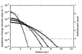
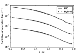
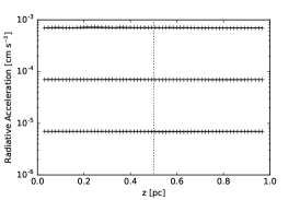
Figure 1: Left panel: Spherically-averaged radiation energy density profiles in the radiative diffusion test in Section 3.1. The analytical (solid lines) and the numerical (crosses) solutions are shown at four different times, $(1,\,4,\,6,\,10)\times 10^{10}\,\mathrm{s}$. The dashed line and the right axis show the refinement level. The middle and right panels show radiative acceleration profiles in the $z$-direction for the plane-parallel slab in Section 3.2. The solid lines and crosses are the results with and without DDMC enabled, respectively. The IMC-DDMC interface is marked with the dotted line at $z=0.5$ pc. Note that no artifact of the IMC-DDMC transition is observed across the interface. Middle panel: Profiles at the optical-thickness-dependent time 0.5 $t_{\rm slab}$ with, from top to bottom, $\tau_{\rm slab}=80,320,3200$. The profiles for $\tau=320$ and 3200 are scaled by factors of 10 and 100 for visual clarity. Right panel: Same as in the middle panel but at steady state.

Similarly, we can divide the equation into energy groups,

$$\frac{1}{c}\frac{\partial J_{1,k}}{\partial t} =\tilde{k}_{{\rm ea},1,k}\tilde{b}_{1,k}c\tilde{u}_{\rm r}$$

$$-[\tilde{k}_{{\rm ea},1,k}+\tilde{\sigma}_{{\rm es},1,k}+\tilde{k}_{{\rm L,if},k}+\tilde{k}_{{\rm R},1,k}]J_{1,k}$$

$$+\left(\frac{\Delta x_{2}}{\Delta x_{1}}\right)\tilde{k}_{{\rm L},2,k}J_{2,k}$$

$$+\frac{1}{\Delta x_{1}}\int^{1}_{0}P_{k}\left(\mu\right)\mu I_{{\rm b},k}\left(\mu\right)d\mu$$

$$+4\pi\frac{\tilde{k}_{{\rm a,}1,k}\tilde{b}_{1,k}}{\tilde{k}_{{\rm p},1}}\sum_{l\neq k}\,\tilde{k}_{{\rm es},1,l}J_{1,l}\Delta\epsilon_{l},$$ (25)

where the reduced effective coefficient $\tilde{\sigma}_{{\rm es},1,k}$ is defined as in Equation (15). This transfer equation for the interface cell differs from the version for interior cells (Equation 2.2.1) in two ways: it contains a revised DDMC-to-IMC leakage opacity, and a new radiation source term that describes the addition of radiation due to IMC-to-DDMC conversion at the boundary of the interface cell.

As in interior cells, we adopt the gray approximation and an isothermal equation of state, the equation can be simplified,

$$\frac{1}{c}\frac{\partial J_{1,k}}{\partial t}= -[\tilde{k}_{{\rm L,if},k}+\tilde{k}_{{\rm R},1,k}]J_{1,k}$$

$$+\left(\frac{\Delta x_{2}}{\Delta x_{1}}\right)\tilde{k}_{{\rm L},2,k}J_{2,k}$$

$$+\frac{1}{\Delta x_{\rm 1}}\int^{1}_{0}P_{k}\left(\mu\right)\mu I_{{\rm b},k}\left(\mu\right)d\mu,$$ (26)

where again, the effective absorption and scattering terms have canceled out.

2.2.4 The IMC-DDMC hybridization

To decide whether radiation transport in a cell should be performed with IMC or DDMC, we compute optical depths of all cells and flag those above a threshold value $\tau_{\rm DDMC}$ as DDMC-active. For Equation (24) to have a valid probabilistic interpretation, we must require $0\leq P(\mu)\leq 1$ with $0<\mu\leq 1$. These conditions impose a minimum threshold optical depth of $\tau_{\rm DDMC}\geq 2.0$. In Section 3 we will show that the exact value of $\tau_{\rm DDMC}$ does not affect the accuracy of the scheme as long as the above criterion is satisfied.

When a DDMC MCP undergoes a leakage event into an IMC cell, it is placed randomly at the cell boundary with a direction sampled isotropically toward the interior of the IMC cell. Once the MCP has entered the IMC cell, it is tracked with the IMC procedure described in Paper I. When an IMC MCP reaches a DDMC cell interface, it is converted into a DDMC MCP with probability $P(\mu)$. In the DDMC cell the converted photon is transported with the DDMC scheme. The non-converted MCPs are returned to the IMC region isotropically and their IMC transport continues. This reflection of MCPs according the chosen form of $W(\mu)$ guarantees that the radiation flux across the IMC-DDMC interface is consistent with the asymptotic diffusion limit, which is an approximate solution of the radiation transfer equation at the interface with radiation impinging on a diffusive, isotropic scattering medium.

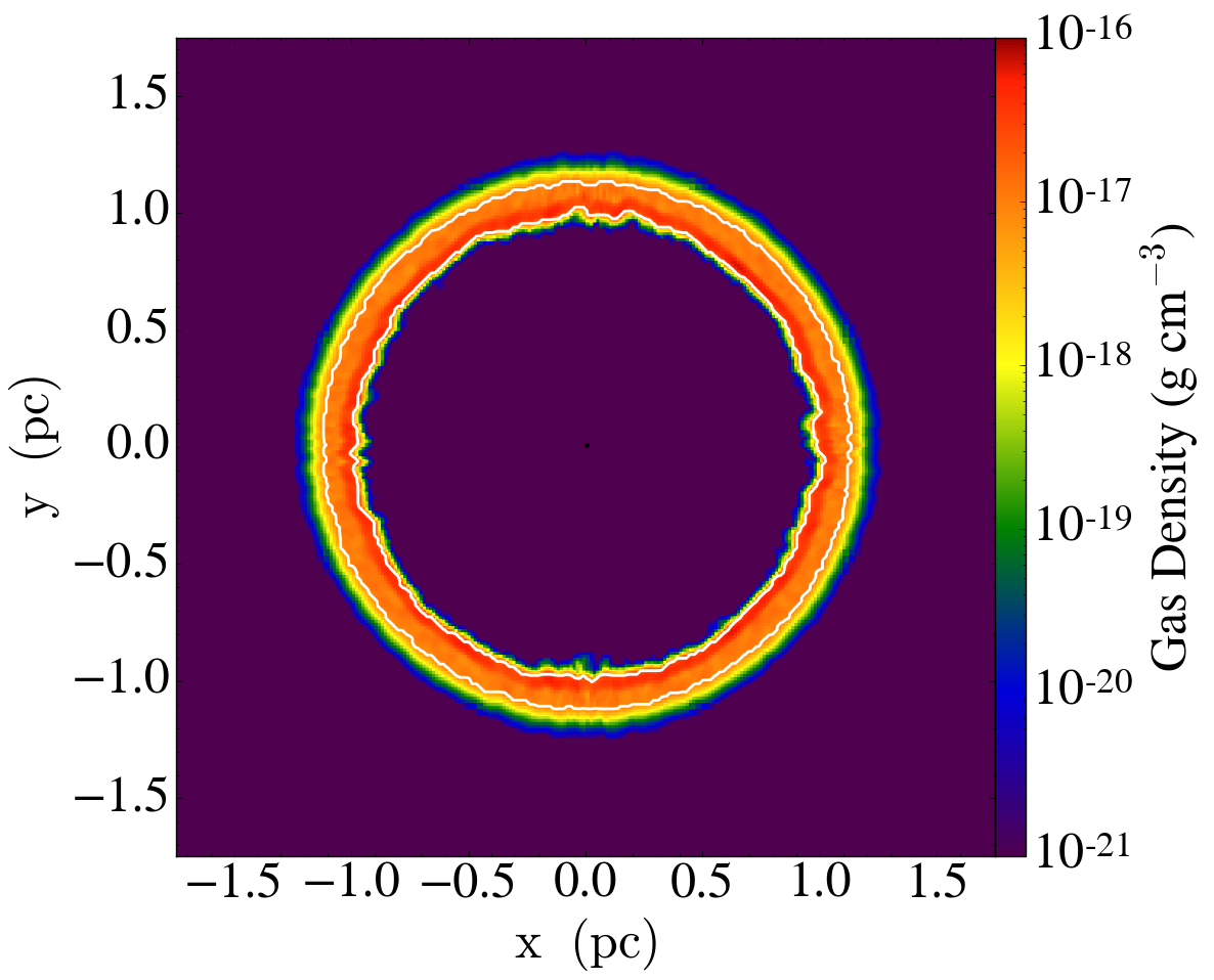
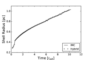
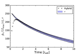
Figure 2: Left panel: Gas density slice at $t=10\,t_{\rm diff}$ in the setup in Section 3.3 in which radiation sweeps up a dense shell from the center of a spherical cloud. The shell has retained spherical symmetry. The region between the thin white contours, dynamically allocated in the course of the simulation, is DDMC-active. Middle panel: Evolution of the radiation-pressure-driven shell’s radius. The slight fluctuations are instability in the numerical extraction of the shell radius from Cartesian data. The plot shows that activating DDMC yields consistent shell dynamics. Right panel: Evolution of the effective radiation force and the optical depth across the dense shell. The blue band represents the $1\sigma$ line-of-sight spread of the optical depth from the discretization of the spherical shell on the AMR grid. At $t\gtrsim t_{\rm diff}$, the diffusive radiation couples closely with the shell.

2.2.5 Momentum deposition

Here we present our scheme for momentum deposition from radiation on gas. Because we treat the gas as isothermal, energy exchange reduces to momentum deposition. In Paper I, we tallied the momentum deposition from individual effective scattering events within a cell,

$$\Delta\mathbf{p}_{\rm es} =-\sum_{\text{eff.\,scatt.}(i)\in\text{cell}}p_{i}(\mathbf{n}^{\prime}_{i}-\mathbf{n}_{i})\simeq\sum_{\text{eff.\,scatt.}(i)\in\text{cell}}p_{i}\mathbf{n}_{i},$$ (27)

where $p_{i}$ denotes the magnitude of the momentum of MCP $i$ and the sum is over all scattering events that occur inside the cell during $\Delta t$. Each event randomizes the direction of the MCP $\mathbf{n}_{i}\rightarrow\mathbf{n}^{\prime}_{i}$. The approximate equality follows from the statistical isotropy of $\mathbf{n}^{\prime}_{i}$.

In optically thin regions, this event-based momentum exchange estimator is noisy. To reduce the noise in IMC regions we adopt a commonly used path-length-based estimator for momentum deposition (Lucy, 1999; Hykes & Densmore, 2009; Harries, 2015; Roth & Kasen, 2015; Smith et al., 2017b)

$$\Delta\mathbf{p}_{\rm es,IMC} =\frac{k_{\rm es}}{c}\sum\epsilon_{i}c\delta t_{i}\mathbf{n}_{i},$$ (28)

where the sum is over all the piecewise paths MCPs execute within the cell.

In DDMC regions where MCPs are not transported with piecewise paths Equation (28) does not apply. We follow Densmore et al. (2007) to evaluate the momentum deposition by averaging the radiation fluxes across cell faces in each grid direction,

$$\Delta\mathbf{p}_{\rm es,DDMC} =\frac{1}{2c}k_{\rm es}\left(F_{-1/2}+F_{+1/2}\right)\Delta t\Delta V,$$ (29)

where $\Delta V$ is the volume of the cell and $F_{\pm 1/2}$ are the net interfacial radiation fluxes due to leakage and IMC-to-DDMC conversion (‘crossing’) events,

$$F_{\pm 1/2}=\sum_{\text{crossing}(i)\in\pm\text{face}(j)}\frac{d_{i}\epsilon_{i}}{\Delta A_{j}\Delta t}.$$ (30)

Here, $\epsilon_{i}$ is the energy of the face-crossing MCP, $d_{i}=\pm 1$ for leakage/conversion towards to the right (upper sign) and left (lower sign) of the cell, $\Delta A_{j}$ is the area of the cell face, and the sum includes all leakage/conversion events across the face. Similar to Paper I, the momentum deposition tallied during the radiation transport is used to construct the source terms for the hydrodynamical updates

$$\mathbf{S}=\frac{\Delta\mathbf{p}_{\rm es,IMC}+\Delta\mathbf{p}_{\rm es,DDMC}}{\Delta t\Delta V}.$$ (31)

and

$$cS_{0}=\mathbf{v}\cdot\mathbf{S}.$$ (32)

These source terms are deposited as gas kinetic energy and momentum at the end of the hydrodynamic time step according to the same procedure reported in Paper I.

3 Performance tests

To validate the hybrid IMC-DDMC radiation transport scheme we solved a suite of test problems. The radiative diffusion setup in Section 3.1 validates the reliability of tracking the diffusion of radiation across mesh refinement jumps. The plane-parallel setups in Section 3.2 demonstrates the robustness of momentum deposition within IMC and DDMC regions as well as across IMC-DDMC interfaces. The radiation pressure-driven shell sweeping setup in Section 3.3 puts the coupled RHD to test, showing the consistency of the DDMC scheme with the IMC scheme.

3.1 Radiative diffusion across mesh refinement jumps

To test optically thick radiative diffusion across mesh refinement jumps, we simulate a $25\,\text{pc}$ cube filled with a uniform, purely scattering medium with density $\rho=10^{-17}$g cm^-3. The absorption opacity is set to zero and the scattering opacity to a constant value $\kappa_{\rm s}=4$ cm² g^-1. Optical depth across a half of the box width is $\tau_{\rm box}=1540$. Such setup is the standard for validating the diffusion limit of any radiation transport scheme (Commerçon et al., 2011; Harries, 2011; Noebauer et al., 2012). Since the objective is to test the transport of MCPs on a nonuniformly refined grid, we disable momentum deposition and gas dynamics in this test. The radiation does not reach the boundary of the box and thus boundary condition is immaterial.

At $t=0$ s, we insert $E_{\rm init}=2\times 10^{52}$ erg of radiative energy in the form of 320,000 isotropically directed MCPs, all initially at the center of the grid. The grid has the base resolution of $32^{3}$. The center of the box is refined three levels higher and has an effective resolution of $256^{3}$. The smallest cell width is $\sim 0.1$ pc which corresponds to a cell optical depth of $\tau_{\rm cell}=12$. The simulation is run for $10^{11}$ s (5% of the half-domain diffusion time) at a constant time step of $\Delta t=2\times 10^{9}$ s. In this test, DDMC is active in the entire simulation domain.

The left panel of Figure 1 shows spherically-averaged radiation energy density profiles at four different times. The radial dependence of the mesh refinement level shown on the right axis. Note the excellent agreement with the analytical solution (solid lines in the figure; see Paper I). The test also demonstrates that DDMC attains the same level of accuracy with fewer MCPs and on a coarser mesh than the basic Monte Carlo method of Paper I.

$\kappa_{\rm s}$ (cm2 g-1)	$\tau_{\rm box}$	$\tau_{\rm cell,min}$	$\tau_{\rm cell,max}$	IMC runtime (s)	DDMC runtime (s)	Speedup
1	385	3	24	9.6$\times 10^{3}$	1.9$\times 10^{3}$	5.1
4	1540	12	96	3.4$\times 10^{4}$	1.5$\times 10^{3}$	22.4
16	6160	48	385	1.4$\times 10^{5}$	1.0$\times 10^{3}$	137.0

Table 1: Parameters and timing results for the timing test presented in Section 3.4.

3.2 Radiative acceleration of a plane-parallel slab

To test the accuracy of momentum deposition under IMC-DDMC hybridization, we construct a three-dimensional plane-parallel setup with sharp transitions in optical thickness. The objective is twofold, to validate that momentum deposition from radiation to gas is accurate in both the IMC and DDMC regions and to check that there are no spurious discontinuities at IMC-DDMC interfaces.

The simulation domain is a cube with side $L_{\rm slab}=1\,\text{pc}$, with a low density $\rho_{\rm low}=2.6\times 10^{-22}\,\text{g}\,\text{cm}^{-3}$ in one half ($z<0.5$ pc) of the cube and a higher constant density in the other half ($z\geq 0.5$ pc). Specifically, we carry out runs with three choices of the higher density of $\rho_{\rm high}=2.6\times 10^{-18}$, $1.03\times 10^{-17}$, and $1.03\times 10^{-16}$ g cm^-3. Assuming a purely scattering medium with an opacity $\kappa_{\rm s}=20\,\text{cm}^{2}\,\text{g}^{-1}$, the low-density half is an optically thin layer with $\tau(z<0.5\,\rm pc)=0.008$ and the high density half has optical depth $\tau(z\geq 0.5\,\rm pc)=80$, 320, and 3200, respectively. The grid resolution is fixed at 64³. As a result, the single-cell optical depth jumps from $2.5\times 10^{-4}$ to 2.5, 10, and 100 across the $z=0.5\,\text{pc}$ interface in the three runs. A constant vertical radiation flux of $2.54\times 10^{7}\,L_{\odot}\,\text{pc}^{-2}\hat{z}$ is introduced at the $z=0$ face. To test the accuracy of momentum deposition, gas dynamics is again disabled; we simply tally the momentum deposited by the MCPs in each cell.

The middle panel of Figure 1 shows the $z$-profiles of the radiative acceleration of gas at the half-diffusion time of the high-density regions $0.5\,t_{\rm slab}=0.5\,\tau_{\rm slab}(L_{\rm slab}/2)/c$. The DDMC is enabled but the low-density region defaults to pure IMC. The profiles agree with each other and with the pure IMC runs (in the figure they are arbitrarily rescaled for visual clarity). We do not observe any artifacts at the IMC-DDMC interface.

In the $t\rightarrow\infty$ steady state limit, the radiative acceleration of a plane-parallel slab transporting a constant flux is uniform in space. The right panel of Figure 1 shows the steady-state radiative acceleration profiles. The solid lines denote the analytical constant value. In all runs, the accelerations agree with the analytical value within $\leq$ 3%. We have also repeated the simulations with an additional refinement level transition at the IMC-DDMC interface (not shown). Our hybrid scheme handles the radiation transfer equally well with a coincident jump in cell size and optical thickness.

3.3 Radiation pressure driven shell

To test how well the IMC-DDMC hybrid scheme couples to the unsplit HLLC Riemann solver we use for the hydrodynamic update, we let the pressure of radiation injected at the center of an optically thick spherical cloud drive the expansion of a shell of gas. The setup is similar to the radiation pressure test in Rosen et al. (2017, see their Sec. 4.2), except that here we focus on the multi-scattered IR radiation instead of the singly-scattered (i.e., absorbed) UV radiation. Our test also bears similarities with the simulation of Costa et al. (2017). We employ the test to validate three key aspects of the hybrid scheme: proper handling of radiation and momentum deposition in non-plane-parallel geometries, stability of radiation transport with dynamically activated DDMC regions, and accuracy of radiative momentum deposition on gas.

A spherical gas cloud with mass $M_{\rm cl}=1.25\times 10^{6}M_{\odot}$, radius $R_{\rm cl}=1$ pc, and uniform density $\rho_{0}=10^{-17}$ g cm^-3 is placed at the center of a (3.5 pc)³ domain. The cloud is embedded in a uniform low-density $\rho_{\rm bg}=10^{-22}$ g cm^-3 background. A constant dust opacity $\kappa_{\rm d}=8.4$ cm² g^-1 is set throughout. The resulting center-to-edge optical depth of the gas cloud is $\tau_{\rm cl}=\kappa_{\rm d}\rho_{0}R_{\rm cl}=264.2$. As in our research-scale simulations in the next section, the equation of state is isothermal. Gravity is disabled in the test.

A radiation source with a constant luminosity $L_{\rm star}=5.6\times 10^{42}$ erg s^-1 is placed at the center. The stellar radiation exerts a net outward radiation pressure. The resulting supersonic expansion sweeps up a dense shell. We adopt a base resolution of (32)³ and allow two levels of adaptive refinement activated with the standard gas density second derivative criterion. The minimum cell width is $\Delta x\simeq 0.04$ pc. We apply DDMC to cells with optical depths exceeding the threshold $\tau_{\rm thres}=2$. The left panel of Figure 2 shows the slice of gas density through the center at time $t=10$ $t_{\rm diff}$, where $t_{\rm diff}$ is the radiative diffusion timescale across the initial uniform gas cloud $t_{\rm diff}=\tau_{\rm cl}R_{\rm cl}/c$.

The spherical symmetry of the swept-up shell is well-preserved. The small asymmetry arose at the beginning of the simulation when the shell was resolved by only a couple cells. Throughout the simulation, the shell is refined at the highest level. The DDMC-active region is not fixed in space but is allowed to adapt to the local optical density and travels with the expanding shell. The region between the white lines in the left panel of Figure 2 marks where DDMC is active.

To validate the shell dynamics, we repeat the simulation with DDMC disabled and compare the results. The middle panel of Figure 2 shows the evolution of the dense shell’s position in both the IMC-only and the hybrid runs. The shell’s radius is computed as the mass-weighted average of the radius of the gas lying above $25\%$ of the peak density. The position of the shell shows excellent agreement between the IMC-DDMC hybrid run and the pure IMC control run.

Quantity	Value	Units
$M_{\rm box}$	10	$10^{6}M_{\odot}$
$L_{\rm box}$	25	pc
$\rho_{\rm init}$	4.4	10-20 g cm-3
$\Sigma_{\rm init}$	1.6	$10^{4}\,M_{\odot}$ pc-2
$t_{\rm ff}$	0.32	Myr
${\cal M}$	7.5	–
$\Delta x_{\rm min}$	0.02	pc
$r_{\rm soft}$	0.06	pc
$t_{\rm max}/t_{\rm ff}$	1.0	–

Table 2: Simulation parameters used in the cluster formation runs.

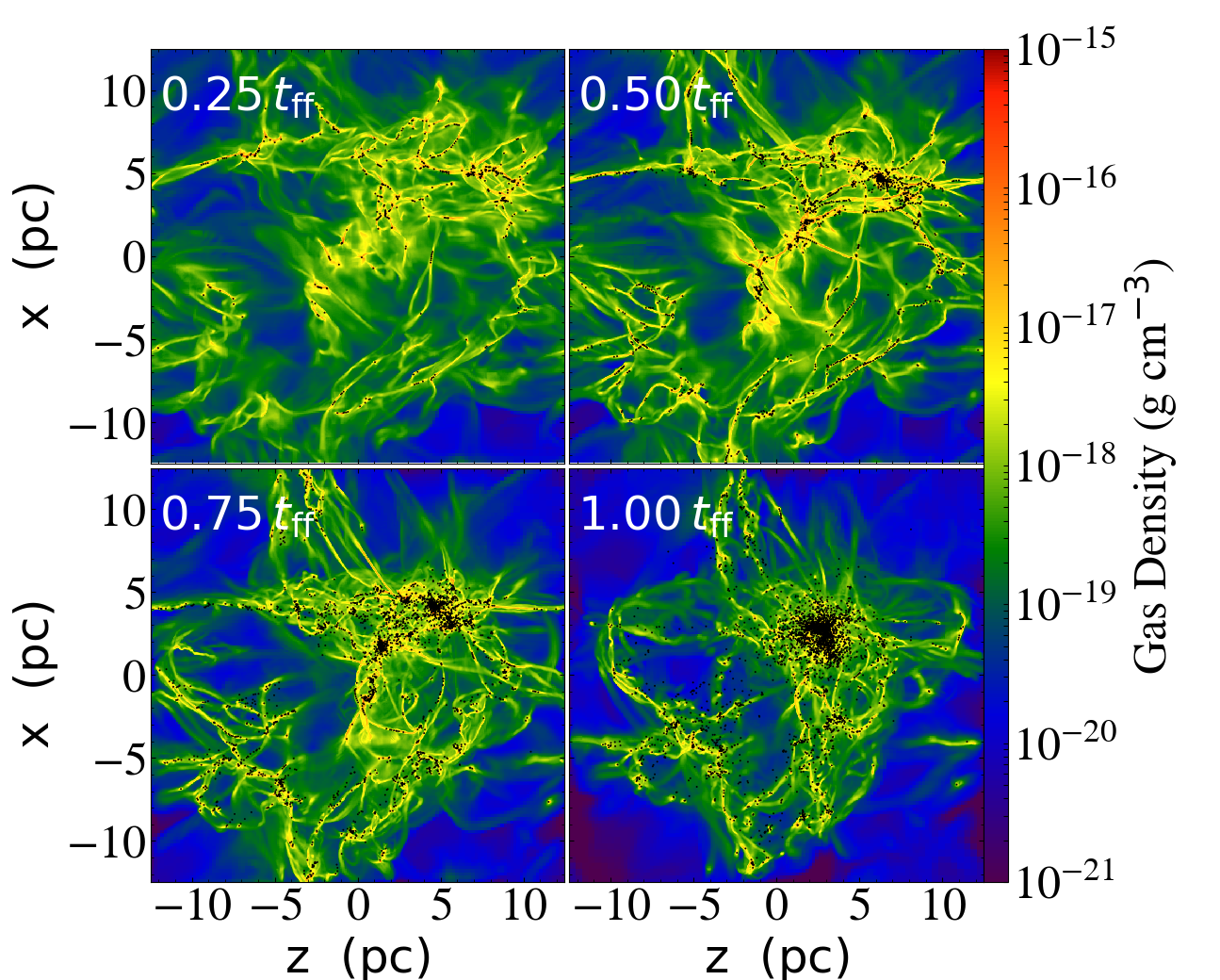
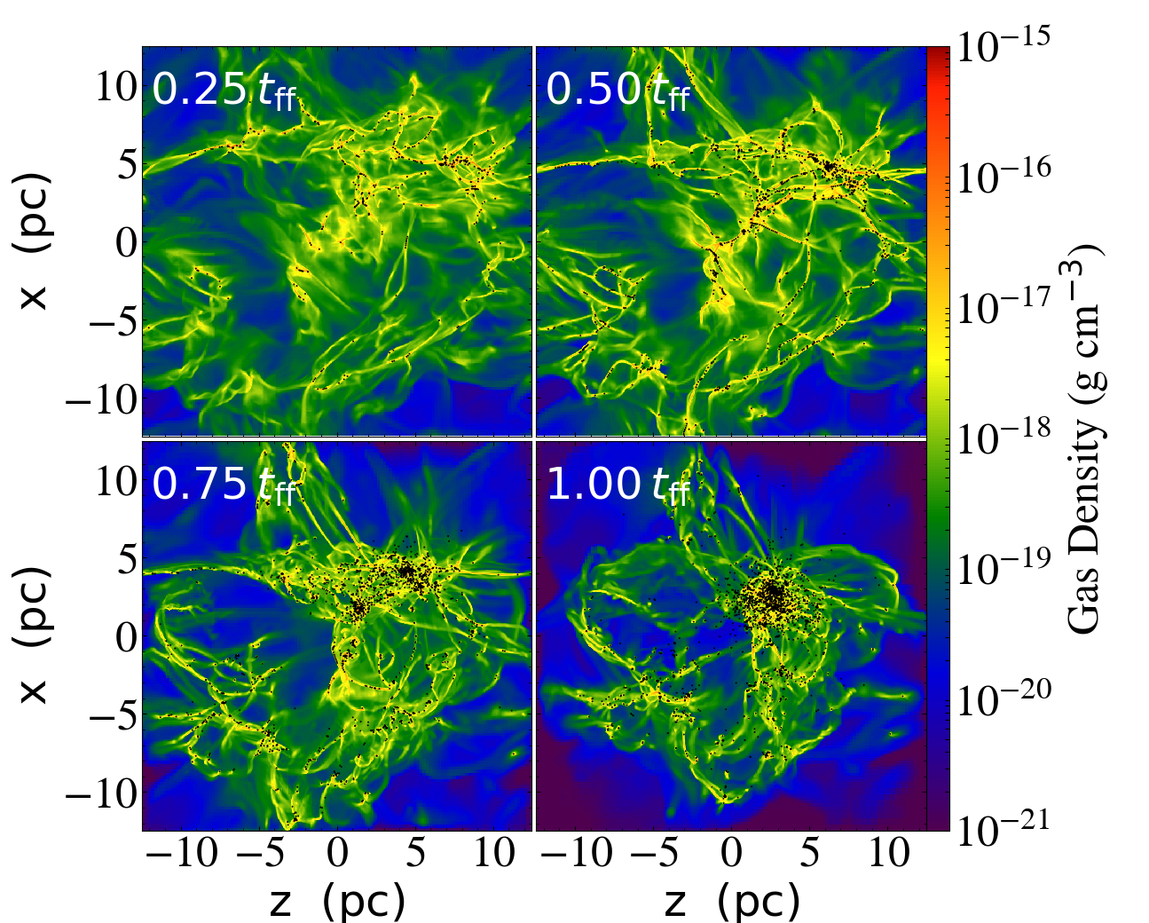
Figure 3: Density-weighted density projections ($\int\rho^{2}dy/\int\rho dy$) of the entire simulation box for the RHD (top panel) and HD runs (bottom panel) at 0.25, 0.5, 0.75, and 1.0 $t_{\rm ff}$, where the free fall time is $t_{\rm ff}=0.3\,\text{Myr}$. Black dots show the projected locations of all sink particles in the simulation.

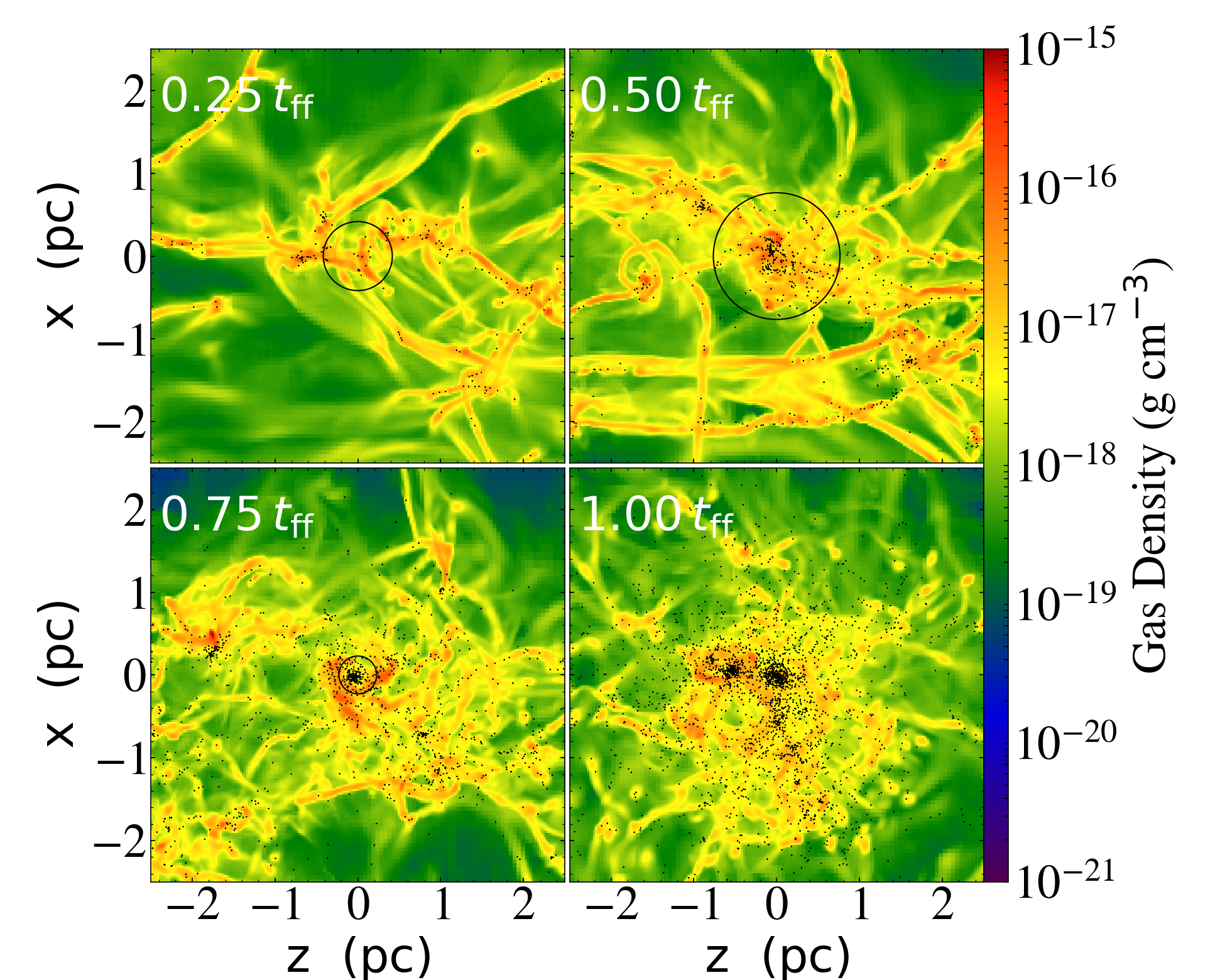
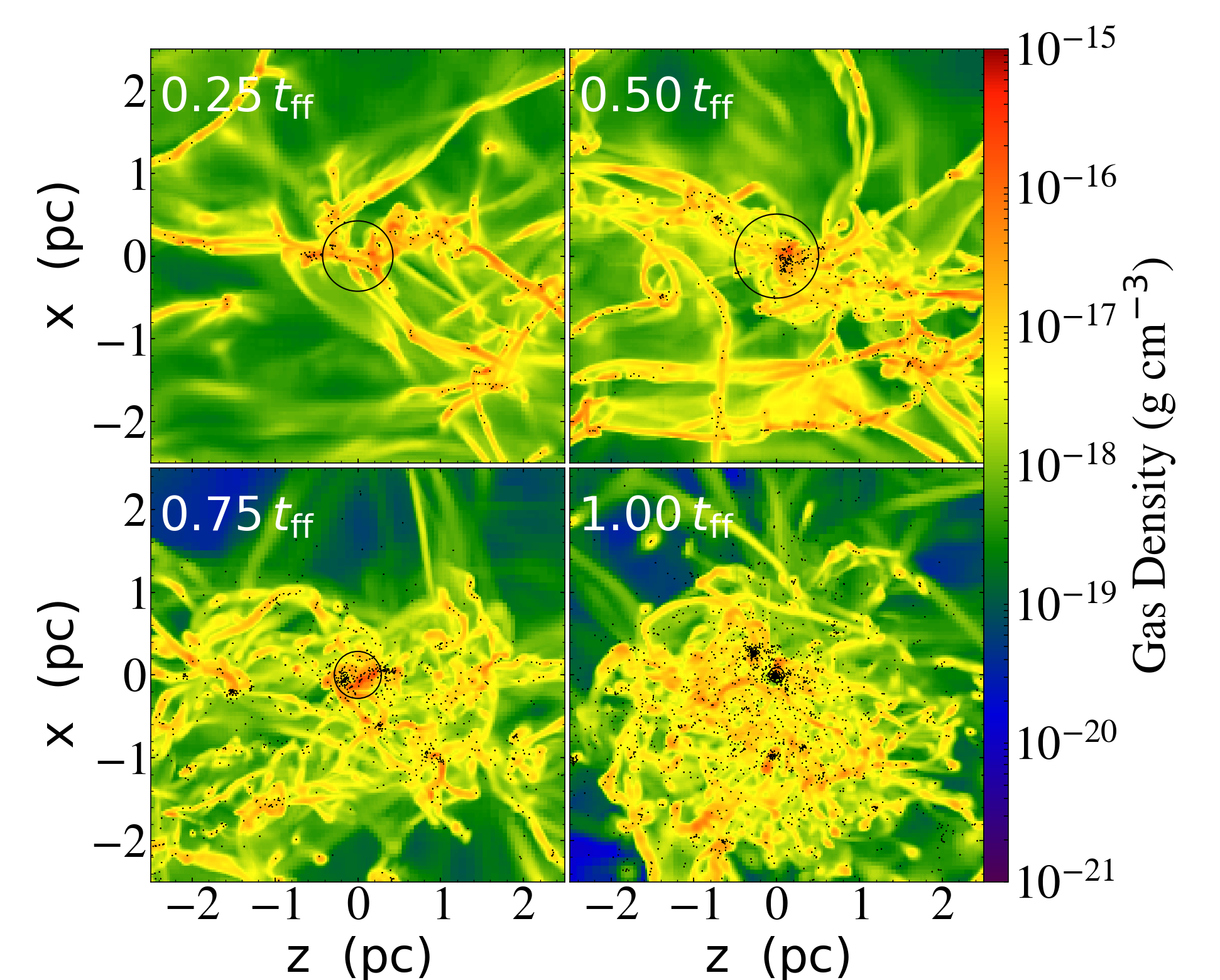
Figure 4: The corresponding (5 pc)² zoomed-in view of Figure 3 centered at the center of mass of the most massive clusters. They show the details of gas and sink distributions around the bases of the global gravitational potentials. Black circles show the size of the cluster’s half-mass radius.

The radiation pressure force is deposited over a layer of finite thickness. To verify accuracy of the momentum coupling, we compare the effective radiative force $\dot{p}_{\rm r}(t)/(L_{\rm star}/c)$ with the instantaneous shell optical thickness $\tau_{\rm sh}(t)$ in the right panel of Figure 2. The blue shaded region shows the $1\sigma$ spread of $\tau_{\rm sh}$ arising from the Cartesian discretization of the spherical shell. The agreement at $t\geq t_{\rm diff}$ is excellent. At $t\leq t_{\rm diff}$, the radiative force has not yet reached its quasi-steady-state level because radiation has not yet diffused through the entire thickness of the shell. This limited momentum flux due to finite travel time of radiation is in line with the results of Costa et al. (2017) who also observed limited momentum coupling when $\tau_{\rm cl}\geq 50$.

In the non-inertial comoving frame of the dense shell, the net outward acceleration by the radiation pressure can be viewed as an effective gravitational acceleration with magnitude $g_{\rm eff}=\dot{p}_{\rm r}/M_{\rm cl}$, where the assumption is that the entire cloud has been swept up into the shell. RTI is expected to grow on the timescale of $t_{\rm RT}=\sqrt[]{\lambda_{\rm RT}/2\pi g_{\rm eff}}$, where $\lambda_{\rm RT}$ is the length scale on which the instability structure grows (Chandrasekhar, 1961). We expect to see RTIs if the dynamical time $t_{\rm dyn}=R_{\rm sh}/v_{\rm sh}$ is longer than $t_{\rm RT}$, where $v_{\rm sh}$ is the shell’s radial velocity. At the end of the test simulation, $\lambda_{\rm RT}\leq 3.6\text{\,pc}$, with a corresponding growth time of $t_{\rm RT}=20$ $t_{\rm diff}$. The length scale is comparable to the size of the system, but we only run the test to 10 $t_{\rm diff}$. On small scales RTI may be suppressed by radiative diffusion, while on larger spatial scales the setup does not yet have enough time to develop significant RTI.

3.4 Timing

To assess the efficiency of the DDMC schem, we repeated the test in Section 3.1 in which radiation is deposited at the grid center at $t=0$ s and allowed to spread radially. With all other parameters fixed, we vary the scattering opacity $\kappa_{\rm s}=1,\,4,\,16$. The wall-clock runtimes required for the simulation to reach $t=10^{11}$ s are recorded. Table 1 summarizes the grid parameters and the timing results. The speedup is defined as the ratio of IMC runtime to the DDMC runtime. DDMC consistently outperforms IMC and the speedup increases at higher opacities. This is a unique advantage of the leakage formalism of DDMC and is reflected in the inverse relation of the leakage opacities to the physical opacities (Equations 11 and 12). At a fixed spatial resolution, leakage of MCPs across cells replaces a larger number of scattering events in regions with higher densities. This enhanced computational efficiency.

4 Simulation methods

In this section we introduce a Monte Carlo simulation of SSC formation to serve as a testbed for our hybrid radiation transport scheme. The simulation is intended to demonstrate the feasibility and effectiveness of the method in research-scale applications. The astrophysical motivation is to examine the effects of the pressure of the reprocessed stellar radiation in the assembly of SSCs. Does the radiation pressure force become competitive with the gravitational force? Does it temper star formation? Does it affect the structure of the resulting SSC?

To simulate SSC formation, we perform a radiation hydrodynamical (RHD) run, and also a radiation-free, purely hydrodynamical (HD) control run in which stellar radiation is disabled. Comparison of the RHD with the HD run allows us to isolate the effects of stellar radiation. Other than for the absence of radiation in the HD run, the two runs have identical parameters and initial conditions. The parameters are explained in what follows and summarized in Table 2.

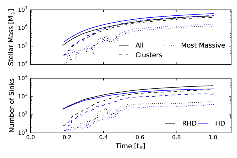
Figure 5: Upper panel: Evolution of the total stellar mass (solid), total stellar mass in clusters (dashed) and in the most massive cluster for the RHD (black) and HD (blue) runs. Lower panel: Evolution of the total sink particle count.

4.1 Preparation of turbulent initial conditions

The gas and gravitational dynamics is computed with the adaptive mesh refinement code flash (Fryxell et al., 2000), version 4.4. We used the unsplit HLLC Riemann solver for the Euler subsystem. Following Federrath et al. (2008) we emulated an isothermal EOS at temperature $T_{\rm EOS}=480\,\text{K}$ via a source term that cancels the $-p\nabla\cdot\mathbf{v}$ term in the internal energy equation. The corresponding speed of sound is $c_{\rm s}=(k_{\text{B}}T_{\rm EOS}/m_{p})^{1/2}\approx 2\,\text{km}\,\text{s}^{-1}$. The isothermal temperature and speed of sound are chosen to match those in SO15 to permit direct comparison.

We prepare the initial density and velocity fields by forcing gas stochastically with gravity disabled. The forcing drives supersonic turbulent fluctuations in the gas. The initial condition preparation via stochastic driving should produce a more realistic initial density field, at least at the high Mach numbers expected in SSC-forming cloud complexes, than the common approach by imposing turbulent velocity fluctuations onto initially spherical, uniform-density clouds.

We start with a total gas mass of $10^{7}\,M_{\odot}$ at uniform density $\bar{\rho}\approx 4.4\times 10^{-20}$ g cm^-3 in a cubic periodic $L_{\rm box}=25$ pc domain. Before turning on gravity, stochastic forcing containing a statistical equipartition mix of solenoidal and compressive forcing modes is applied in the box (see, e.g., Federrath et al., 2008). The forcing is carried out for five turbulence-crossing times; the crossing time is $T=\frac{1}{2}L_{\rm box}/V$, where $V={\cal M}c_{\rm s}$ and ${\cal M}=\langle v^{2}\rangle^{1/2}/c_{\rm s}$ is the mass-weighted average Mach number of the gas flow. In this definition $\langle f\rangle\equiv\sum m_{i}f_{i}/\sum m_{i}$, where $m_{i}$ is the mass in cell $i$ and and $f_{i}$ is the cell-average of quantity $f$. Although gravity is disabled, during the initial stochastic forcing the mesh is adaptively refined following the criterion of Truelove et al. (1997), namely, requiring that the nominal local Jeans length $\lambda_{\text{J}}=c_{\text{s}}\sqrt{\pi/G\rho}$ be resolved by at least four grid cells. The base resolution is $64^{3}$ and we allow four levels of refinement, which translate to a maximum and minimum cell size of $\Delta x_{\rm max}\sim 0.4\,\text{pc}$ and $\Delta x_{\rm min}\sim 0.02\,\text{pc}$, respectively. Before gravity is activated, the Truelove et al. (1997) criterion is satisfied in the entire domain.

The density statistics and mass-weighted velocity dispersion of the turbulent flow reach a statistical steady state after $\sim 2\,T$ when the Mach number is ${\cal M}\sim 7.5$. We verified that the steady-state density is approximately log-normally distributed as expected in isothermal turbulence. The density statistics exhibits deviations from the log-normal shape that are all consistent with Federrath et al. (2008, 2010a).

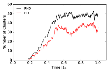
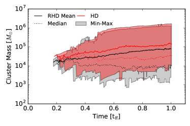
Figure 6: Left panel: Evolution of the total number of star clusters returned from the DBSCAN detection routine in the RHD (black) and the HD (red) run. Right panel: Evolution of the range of cluster mass in the RHD (black) and the HD (red) run. The solid and dotted lines denote the mean and the median mass of all star clusters, and the shaded regions span the minimum and the maximum cluster mass.

4.2 Gravitational hydrodynamics

After the statistical steady state is identified at $5\,T$, we stop the stochastic forcing and activate gravity. We compute the gas self-gravity with the multigrid Poisson solver of Ricker (2008). After gravity is activated, inertial turbulent compression triggers distributed gravitational collapse. The sites of collapse are organized into hierarchical, merging structures, just as in real observed star-forming galactic environments. We track the formation of internally unresolved stellar groups by creating gravitating sink particles from the gas that is too dense for its Jeans length to be resolved. Sink particles are introduced when the gas flow fulfills the joint criteria for subgrid gravitational collapse (Federrath et al., 2010b): the local Jeans length is no longer resolved by $\geq 4$ grid cells even at the highest level of refinement, the flow is converging $\nabla\cdot\mathbf{v}<0$, the gravitational potential has a local minimum, absolute value of cell’s gravitational energy exceeds the sum of the internal and kinetic energies (therefore the cell is gravitationally bound), and there are no pre-existing sink particles within the new particle’s accretion radius $r_{\rm acc}=2.5\,\Delta x_{\rm min}$.

With our parameter choices the maximum density allowed by the Truelove et al. (1997) condition is $\rho_{\rm th}=1.3\times 10^{-17}$ g cm^-3. The sink particles are allowed to accrete gas subject to the same criteria as for sink creation adding the requirement that the accreting gas be gravitationally bound to the particle.

The gravitational force between the sinks and between the sinks and gas is computed by direct summation. Inside a small radius $r_{\rm soft}$, the sink-sink force is softened by spline kernel interpolation (Federrath et al., 2010b). The sink-gas force is softened linearly within the same radius. The gravitational acceleration on a cell due to a sink particle switches continuously from the inverse-square law, $a_{\rm grav}=-GM_{\rm sink}/r^{2}$, outside the softening radius to the linear scaling $a_{\rm grav}=-GM_{\rm sink}r/r_{\text{soft}}^{3}$ inside. We do not allow merging of sink particles; once formed, the sinks remain in the simulation. After about a few thousand sinks have formed, the cost of direct gravitational force summation become significant. To reduce this cost, we approximate the sink-gas gravitational calculation by aggregating the force from the particles in distant blocks in the spirit of the Barnes & Hut (1986) approximation. (The blocks are the basic computational units aggregating 16³ cells each.) Each block is subjected to a solid-angle test comparing $L^{2}_{\rm block}/d^{2}$, where $d$ is the particle to block center distance, to a constant value $1.53\times 10^{-3}$. With this criterion the aggregation scheme is applied when a block at the highest refinement level is separated from a particle by a distance $d\geq 5\,\text{pc}$.

4.3 Sink particles as radiation sources

Each sink particle represents a group of stars sampling the entire stellar initial mass function (IMF). We implement a simple prescription for sink particle radiative output by fixing the luminosity-to-mass ratio to $L_{\rm sink}/M_{\rm sink}=3000$ erg s^-1 g^-1. This ratio is chosen slightly higher than the value $\sim 2000\,\text{erg}\,\text{s}^{-1}\,\text{g}^{-1}$ predicted by the Starburst99 models (Leitherer et al., 1999) for the Kroupa (2001) IMF at solar metallicity. The optimistic ratio is chosen to probe upper limits of dynamical forcing by radiation pressure. The dust opacity is fixed at $\kappa_{\rm dust}=20\,\text{cm}^{2}\,\text{g}^{-1}$, about the value at which SO15 found radiation pressure started to significantly influence star formation efficiency. The opacity is consistent with the Planck mean opacity of stellar-radiation-heated, warm ($100$–$500\,\text{K}$) dusty gas at $2$–$3$ times the solar metallicity (e.g., Semenov et al., 2003; Kuiper et al., 2010). With these choices, the Eddington ratio is $f_{\rm Edd,sph}=\kappa_{\rm dust}(L/M)/(4\pi cG)\simeq 2.4$. A heuristic cell optical thickness threshold of $\tau_{\rm DDMC}=5$ is set to activate the DDMC acceleration scheme.

Radiation MCPs are transported across processors using the moveParticles subroutine in flash. The subroutine uses asynchronous, non-blocking message passing interface (MPI) calls to minimize communication overhead. By default, flash estimates the total amount of work by assigning one unit of work to non-leaf blocks and two units to leaf blocks. It then distributes approximately equal amount of work to each processor. Sink particles are mapped to the processors hosting the blocks that contain them. As a simulation proceeds, the clustering of sink particles can impose an asymmetric load on isolated processors by encumbering them with unbalanced gravitational and radiation transport calculations. To alleviate load imbalance, we modified the work estimate in the subroutine amr_refine_derefine to add ten units of work to the hosting block for each sink particle. This work allocation heuristic improved workload balance.

To avoid giving radiation pressure a non-physical advantage over the artificially softened gravity, radiative acceleration is softened in the same way as gravity, by multiplying the amount of momentum transferred from the MCP to the gas cell with the attenuation factor $r^{3}/r^{3}_{\rm soft}$, where $r$ is the distance from the MCP to the cell center. Radiation MCPs are removed when they are more than $0.25\,L_{\rm box}=6.25\,\text{pc}$ away from their source sinks.

4.4 Cluster identification

Recall that sink particles represent unresolved, bound stellar groups. As the simulation progresses, the sinks become organized in viralizing clusters. To characterize sink particle membership in clusters, we adopt the density-based clustering algorithm DBSCAN (Ester et al., 1996) implemented in the scikit-learn Python library. The two key parameters are eps $=0.5\,\text{pc}$ and n_samples $=10$, which are the maximum distance between any sinks in a cluster and the minimum number of sinks to qualify to be a cluster, respectively. These resolution-dependent values were chosen heuristically. We will find that in clusters, stellar mass exceeds gas mass; therefore, in what follows we regard the center of mass of all the sinks in a cluster as the cluster’s center. DBSCAN is also identifies sinks not assigned to any cluster; we refer to them as ‘field sinks’.

5 Results

In this section, we first characterize star formation and massive cluster properties in the simulations. Then we examine the impact of radiation pressure on star and cluster formation.

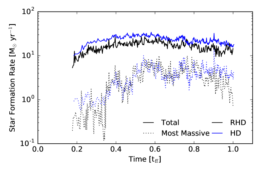
Figure 7: Evolution of the total SFR (solid) and inside the most massive cluster (dotted) in the RHD (black) and HD (blue) run. The SFR includes the gas accretion onto existing sink particles and the creation of new sinks. In both simulations accretion onto existing sinks dominates the SFR.

5.1 Star formation

The very first sink particles form shortly after gravity has been activated in sites where flow convergence compresses gas to high density. Figure 3 shows the density-weighted density projections of the entire simulation domain along the $y$-axis at $(0.25,\,0.5,\,0.75,\,1.0)\,t_{\rm ff}$, in the RHD and HD runs. In both runs, the first sink particles form in the center of the densest gas clump after $\sim 5.4\,\text{kyr}\simeq 0.017\,t_{\rm ff}$ from the moment gravity was switched on. Sink particles subsequently form along the gas filaments as seen in the $t=0.25\,t_{\rm ff}$ and $0.5\,t_{\rm ff}$ snapshots. The simulations are carried out to $1\,t_{\rm ff}\sim 0.3\,\text{Myr}$. Gas flow morphology and visual sink particle clustering in the two runs remains similar on large scales. Figure 4 shows the corresponding zoomed-in views of the most massive clusters and their half-mass radii. Sinks form along the filaments but a large scale gravitational field then pulls them into the nearby virialized clusters. The collapsing structures have angular momentum and rotate.

The top panel of Figure 5 shows the total stellar mass growth in both runs. The stellar masses grow smoothly to reach $4.6\times 10^{6}$ ($6.2\times 10^{6}\,M_{\odot}$) in the RHD (HD) run. These final stellar masses correspond to box-wide star formation efficiencies of 46% (62%). The total stellar mass in the HD run is consistently $\sim 1.3$–$1.5$ times higher than in the RHD. Section 5.3 attributes this effect to radiation pressure. Since our sinks do not merge, the number of sinks also increases smoothly to a final total of $\sim 3900$ ($\sim 2600$) in the RHD (HD) run. The lower panel of Figure 5 shows the evolution of sink particle counts. In Section 5.2 we ascribe the larger number of sinks in the RHD simulation to the radiation suppressing accretion onto existing sinks while leaving more gas to collapse into new sinks. Indeed the average sink mass is systematically higher in the radiation-free HD run.

We follow the procedure described in Section 4.4 to group sink particles into clusters and a separate unclustered population of field sinks. Since each sink is itself an unresolved stellar group, the field sinks should not be construed as isolated stars, but are small clusters. Natural compact clusters dynamically evaporate but our subgrid prescription does not model sink evaporation. The most massive clusters acquire a significant fraction of the total stellar mass by $t=0.5\,t_{\rm ff}$ and have stellar masses $1.3\times 10^{6}$ ($1.6\times 10^{6}\,M_{\odot}$) at the end of the RHD (HD) simulations. The fluctuations of the measured stellar mass in the most massive cluster are an artifact of unstable cluster membership identification during cluster merging. In Figure 6, we show the evolution of the cluster count and the cluster mass range. The cluster mass ranges between $\sim 10^{3}\,M_{\odot}$ and $\sim 10^{6}\,M_{\odot}$. The low median cluster mass shows that most of the clusters have low masses.

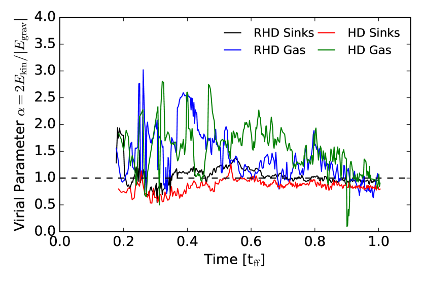
Figure 8: Evolution of the virial parameter $\alpha_{\rm vir}=2E_{\rm kin}/|E_{\rm grav}|$ of the stellar and gas components inside the most massive cluster in the two runs. In both runs, the star clusters represented by the sink particles virialize about 0.6 $t_{\rm ff}$ after the formation of the first sink and maintain the virialized state while they grow in mass. The gas component is bound ($\alpha_{\rm vir}<2$) to the sink cluster after about 0.5 $t_{\rm ff}$.

A comparison of the global star formation rates (SFR) in both runs is shown in Figure 7. The SFRs account for the formation of new sinks and the accretion of mass onto existing sinks. Throughout the simulations, gas accretion on existing sinks dominates new sink creation. The global SFRs inside the simulation boxes increase sharply at early times to $\geq 10\,M_{\odot}\,\textrm{yr}^{-1}$ within $\sim 0.2\,t_{\rm ff}$ and peak at $\sim 20\,M_{\odot}\,\textrm{yr}^{-1}$ and $\sim 30\,M_{\odot}\,\textrm{yr}^{-1}$ in the RHD and HD runs, respectively. The SFRs then decline slightly, but the strong gravitational collapse still keeps the SFRs above 10 $M_{\odot}\,\textrm{yr}^{-1}$ in both runs. Figure 7 shows that although the global SFR is $\sim$1.2–2 times higher in the non-radiative run, the SFRs inside the most massive clusters are almost identical between the two runs. This is the first indication that radiation is not deleterious to a massive cluster’s—SSC’s—ability to continue forming stars. If we further decompose the total SFR into the clusters vs. the field, we find that similar to the trend seen in the stellar mass, clusters contribute a larger fraction to the total SFR in the RHD run. As sinks become incorporated in virialized clusters where they move fast and are subject to frequent two-body encounters that can scatter them to still higher velocities, an increasing fraction of sinks, especially those in clusters, ceases to accrete. While particles prefer to accrete outside clusters where they move slowly relative to gas, it seems that it is also outside clusters that radiation pressure has the greatest impact on the local gas density and separately suppress accretion.

5.2 Properties of clusters

In this section we analyze the properties of the clusters in the simulations. Figure 8 shows the virial parameter $\alpha_{\rm vir}=2E_{\rm kin}/|E_{\rm grav}|$, where $E_{\rm kin}$ and $E_{\rm grav}$ are the total kinetic and gravitational potential energy of the gas or sink component inside the half-mass radius. Since the stellar mass largely dominates over the gas mass, we do not include the contribution from gas self-gravity in the $E_{\rm grav}$ term. Independent of whether radiation pressure is enabled, the stellar component virializes quickly, at about 0.6 $t_{\rm ff}$. The gas component virializes later and remains gravitationally bound to the stellar component.

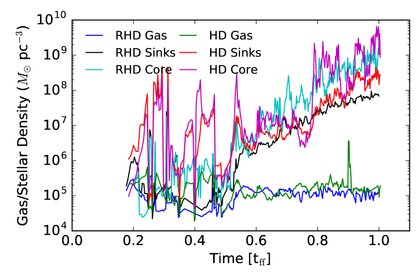
Figure 9: Evolution of stellar and gas densities measured within the half-mass radius of the most massive cluster. Since the massive cluster is centrally-concentrated, we also estimate the peak stellar density by averaging the density of 10 sink particles closest to the cluster’s center of mass. Stellar mass dominates gas mass during most of the simulations. The peak stellar density reaches $\sim 10^{8}\,M_{\odot}\,\textrm{pc}^{-3}$ where runaway stellar merging can produce a very massive star. The gas density is near-constant at $1-2\times 10^{5}\,M_{\odot}\,\textrm{pc}^{-3}$ after 0.5 $t_{\rm ff}$.

Figure 9 plots the gas and stellar density within the half-mass radius of the most massive cluster. By $t\simeq 1\,t_{\rm ff}$ the gas density in both runs saturates at a near-constant value $\rho_{\rm gas}\approx 10^{5}\,M_{\odot}\,\text{pc}^{-3}$. The stellar density reaches $\rho_{*}\approx 6\times 10^{7}\,M_{\odot}\,\textrm{pc}^{-3}$ in the RHD run and $\rho_{*}\approx 2\times 10^{8}\,M_{\odot}\,\textrm{pc}^{-3}$ in the HD run. The increase of stellar density near the end of the simulation is likely the result of dynamical relaxation. The peak stellar density is lower in the RHD run. From this we can conclude that radiation pressure does seem to influence cluster structure. However, radiation does not limit the density as proposed in the literature (Hopkins et al., 2010). Interestingly, stellar density is such that collisional formation of very massive stars (VMSs) is expected (Moeckel & Clarke, 2011).

In Figure 9 we further estimate the core stellar density in clusters by measuring density in the sphere enclosing 10 sink particles closest to the cluster center. The peak density reaches $8\times 10^{8}\,M_{\odot}\,\text{pc}^{-3}$ by the end of the simulations. Thus, radiation pressure does not seem to have a large impact on the final peak density. Note that this extreme stellar density is reached very early-on in the clusters’ evolution at $t=1\,t_{\rm ff}=0.3\,\text{Myr}$, well before the arrival of the first supernovae.

Since the sink particles exhibit a significant mass spread, we expect mass segregation should occur. Mass segregation can shorten the core collapse time scale below the nominal two-body relaxation time. Since sink particle masses are resolution-dependent quantities, the degree of mass segregation in the simulations is not predictive of mass segregation in real clusters. Nonetheless, to understand the simulation we must quantify the effect of segregation. We estimate it using the widely adopted minimum spanning tree (MST) method (Allison et al., 2009; Olczak et al., 2011; Maschberger & Clarke, 2011). An MST is the minimum total edge length of an undirected acyclic graph connecting a set of sinks. Our analysis follows the standard approach to quantify the level of mass segregation in a star cluster using the MST ratio $\Lambda_{{\rm MSTR},m}=\bar{l}_{{\rm random},m}/l_{{\rm massive},m}$, where $l_{{\rm massive},m}$ is the total edge length of the MST connecting the $m$ most massive sinks in the cluster, and $\bar{l}_{{\rm random},m}$ is the same but averaged over 100 sets of $m$ sinks randomly selected independent of sink mass. When $\Lambda_{{\rm MSTR},m}>1+{\cal O}(1/\sqrt{m})$, the $m$ most massive sinks are likely to be sampling a more compact region than the region sampled by the whole cluster. We pick $m=10$ and construct the MST using the csgraph implementation of the Scipy library. From $t\geq 0.5$ $t_{\rm ff}$ onwards, we observe a mean ratio of $\Lambda_{\rm MSTR}\sim 1.6-1.7$ in both runs, suggesting a moderate degree of mass segregation. These values are not sensitive to the precise choice of $m$ for $10\leq m\leq 200$.

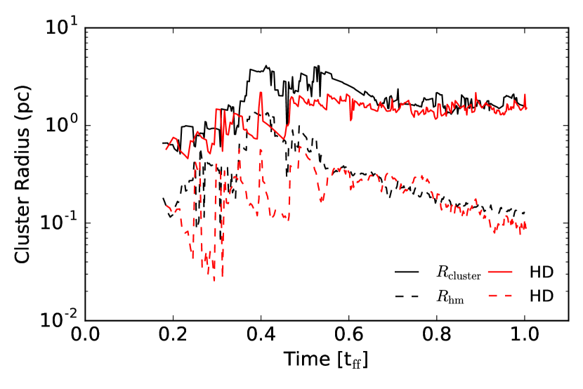
Figure 10: Evolution of the most massive cluster radius and the half-mass radius in both runs.

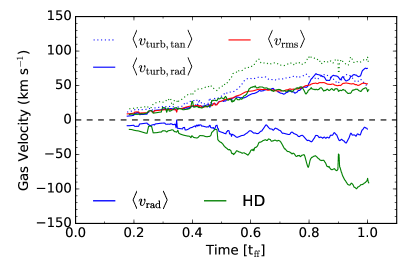
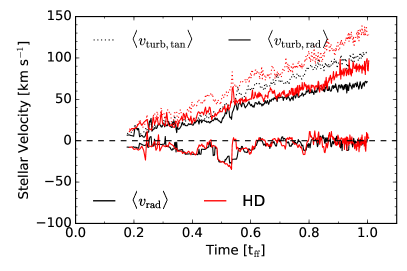
Figure 11: Left panel: Evolution of mass-weighted gas velocity moments in Section 5.2, measured inside a 1 pc sphere centered on the most massive cluster. The red solid line is the one-dimensional velocity dispersion. Right panel: Evolution of the corresponding particle-mass-weighted sink particle velocity moments as indicated in the legend.

Radio and millimeter observations provide access to the kinematics of massive star- and cluster-forming clumps at high angular resolution and sensitivity (Herrera & Boulanger, 2017; Ginsburg et al., 2017; Turner et al., 2017). To enable the comparison of our modeling to observations, we investigate the velocity structure of the gas and stellar component in the clusters. The left panel of Figure 11 shows the evolution of the mass-weighted mean radial streaming velocity and the mass-weighted root-mean-square radial and tangential turbulent gas velocities in spheres centered on the most massive star clusters

$$\langle{v}_{\rm rad}\rangle =\frac{\sum_{j}m_{j}\mathbf{v}_{j}\cdot\hat{\mathbf{r}}}{\sum_{j}m_{j}},$$ (33)

$$\langle{v}_{\rm turb,rad}\rangle =\sqrt{\frac{\sum_{j}m_{j}|\mathbf{v}_{j}\cdot\hat{\mathbf{r}}-\langle v_{r}\rangle\hat{\mathbf{r}}|^{2}}{\sum_{j}m_{j}}},$$ (34)

$$\langle{v}_{\rm turb,tan}\rangle =\sqrt{\frac{\sum_{j}m_{j}(|\mathbf{v}_{j}|^{2}-|\hat{\mathbf{r}}\cdot\mathbf{v}_{j}|^{2})}{\sum_{j}m_{j}}},$$ (35)

where $m_{j}$ and $\mathbf{v}_{j}$ are the mass and mean-cluster-motion-subtracted velocity in cell $j$. The sums are taken over the cells with centers within 1 pc from the cluster center.

The HD and RHD runs differ in the evolution of the mass-weighted average radial streaming velocity $\langle v_{\rm rad}\rangle$. The infall velocity in the radiation-free run becomes as high as $\sim 100\,\text{km}\,\text{s}^{-1}$, whereas in the run with radiation it never exceeds $\sim 30\,\text{km}\,\text{s}^{-1}$. Since this difference cannot be explained by the radiation-free run’s higher mass and central density, it seems that radiation pressure is slowing down radial infall. The radial turbulent velocities in the two runs are comparable until $t\sim 0.8\,t_{\rm ff}$, whereupon in the RHD run the radial turbulent velocity reaches $\sim 60$ km s^-1 and the HD run remains at a somewhat lower value $\sim 40$ km s^-1. The tangential velocity $\langle v_{\rm turb,tan}\rangle$ is systematically higher in the HD run. In Figure 11, right panel, we plot the equivalent kinematical indicators, but for the sink particles. Note that after the RHD cluster virializes at $t\sim 0.6$ $t_{\rm ff}$, its particle-mass-weighted mean radial streaming velocity approximately vanishes, as expected. The velocity dispersions are larger in the HD run because the radiation-free run converts more gas into sink particles and has a larger virial mass. We summarize properties of the final most massive cluster in the RHD run in Table 3.

Property	Value
Stellar mass	$1.3\times 10^{6}\,M_{\odot}$
Residual gas mass	$1.4\times 10^{5}\,M_{\odot}$
Fiducial cluster radius	$1.6\,\text{pc}$
Half-mass radius	$0.1\,\text{pc}$
Stellar velocity dispersion	$73\,\text{km}\,\text{s}^{-1}$
Gas velocity dispersion	$53\,\text{km}\,\text{s}^{-1}$
Star formation rate	$1\,M_{\odot}\,\text{yr}^{-1}$

Table 3: Properties of the most massive cluster at the end of the RHD run, $0.3\,\text{Myr}$ after the beginning of star formation.

5.3 The impact of radiation pressure

Since star formation efficiency is lower in the RHD run than in the radiation-free HD control run, and since both simulations are artificially set isothermal, one can conclude that to a degree, radiation pressure inhibits star formation. However, although we chose optimistically high values of dust opacity and stellar luminosity-to-mass ratio, radiation pressure did not truncate star formation. Even at the end of the RHD simulation, gas accretion onto sink particles persists and new sinks are forming. Regardless of the epoch or region within the simulation, the SFR is depressed by at most a factor of 2 in the RHD compared to the HD run. Since this is at odds with certain theoretical predictions (Murray et al., 2010; Kim et al., 2016), in what follows we closely examine the transport of stellar radiation.

In the core of the most massive star cluster formed in the RHD simulation, gas distribution is highly inhomogeneous. This allows radiation to leak out through low-density channels. The leakage reduces the coupling of the radiation pressure force with the dense clumps that contain most of the gas mass. The radiation-matter anti-correlation in strongly inhomogeneous gas limits radiation pressure’s effect on the gas supply for star formation. The anti-correlation was observed in previous multi-dimensional simulations of star cluster formation (Skinner & Ostriker, 2015), plane-parallel radiation-pressure-driven outflows (Krumholz & Thompson, 2012, 2013; Davis et al., 2014; Rosdahl & Teyssier, 2015; Tsang & Milosavljević, 2015; Zhang & Davis, 2017) and massive star envelopes (Jiang et al., 2015).

Figure 12 plots volume- and mass-weighted spherically-averaged radiation pressure acceleration in the RHD run. The spherical averaging is done around the center of the most massive cluster at $t=t_{\rm ff}$. Also shown is the spherically symmetric analytical profile for an equivalent central source:

$$a_{\rm rad,approx}(r)=\frac{\kappa_{\rm dust}\sum_{i}{L_{i}}}{4\pi r^{2}c},$$ (36)

where the summation runs over the sink particles within $r$. While the volume-weighted radiative acceleration closely follows the analytical estimate, the mass-weighted acceleration, a proxy for the actual radiation pressure that the gas experiences, consistently lies below the analytical prediction. To visualize the effect of radiation-matter anti-correlation, we also overlay the radial profiles of the radiative acceleration on the color rendering of cell optical depths. Most of the gas with $\tau_{\rm cell}>1$ experiences a substantially reduced radiation pressure force whereas the gas with $\tau_{\rm cell}<1$ is more strongly accelerated than the analytical estimate.

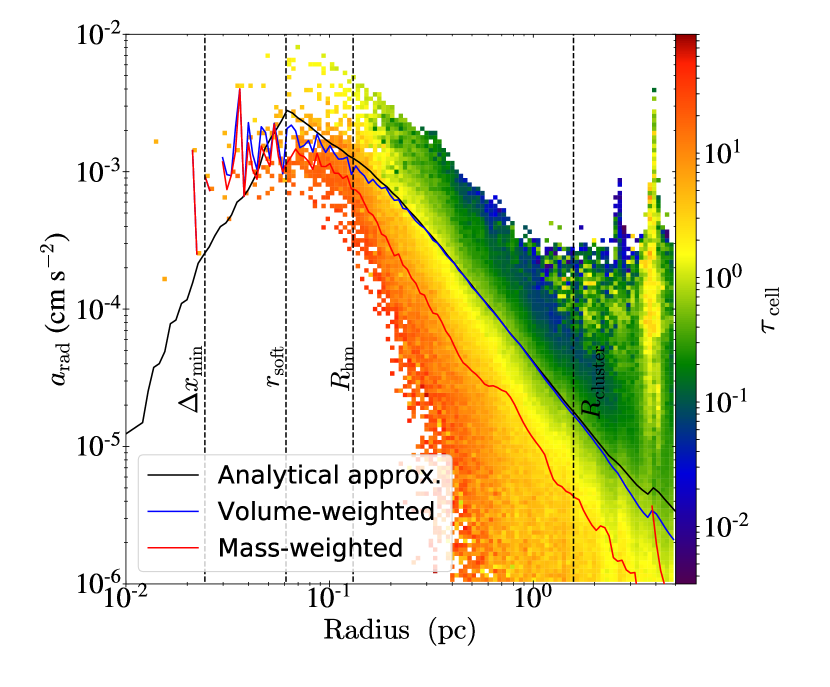
Figure 12: Radiative acceleration and cell optical thickness as a function radius from the center of the most massive cluster at $t=t_{\rm ff}$ in the RHD run. The pixel color represents the average cell optical depth. The black solid line is the analytical acceleration assuming that stellar point sources are at the center. The red and blue lines are, respectively, profiles of mass- and volume-weighted radiative acceleration. The vertical dashed lines, from left to right, mark the minimum cell width, softening radius, cluster’s half-mass radius, and cluster radius.

This inhomogeneity-enabled reduction in the effective radiation pressure persists throughout the simulation. We define mass- and volume-weighted Eddington ratio within a sphere of radius $R$

$$f_{\rm Edd}(R)=\frac{\langle a_{\rm rad}\rangle_{R}}{\langle a_{\rm grav}\rangle_{R}},$$ (37)

where the averages, weighted either by the cell mass or volume, are over the cells within the sphere. We only include sink-gas gravitational attraction in the $a_{\rm grav}$ term; it is a good approximation as stellar mass dominates. Figure 13 shows the evolution of the average Eddington ratios around the most massive cluster computed within three radii: the cluster’s time-dependent half-mass radius, 1 pc, and 2 pc. It shows that the radiation-matter anti-correlation renders the mass-weighted ratio sub-Eddington whereas the volume-weighted ratio is super-Eddington and close to the spherically-symmetric value $f_{\rm Edd,sph}$ (Section 4.3).

For radiation pressure to temper star formation, the radiative acceleration not only has to exceed the local gravitational acceleration, but also has to cancel the inertia of the already infalling gas. The left and middle panels of Figure 14 show the Eddington ratio $f_{\rm Edd,cell}$ and gas mass as a function of $\tau_{\rm cell}$ and radial streaming elocity $v_{\rm rad}$ for cells within 2 pc from the most massive cluster center at $t=t_{\rm ff}$. The radiation-matter anti-correlation is clear---almost all of the super-Eddington cells are optically thin $\tau_{\rm cell}<1$ (top left of left panel), and most of the optically thick gas mass with $\tau_{\rm cell}>1$ is sub-Eddington. In addition, a fraction of optically thin cells is being radiatively accelerated in an outflow. The mass-weighted average radial velocity in the outflowing and inflowing cells is, respectively, 56 km s^-1 and $-49$ km s^-1. The escape velocity from the cluster radius is 90 km s^-1 and thus, on average, the outflowing gas remains gravitationally bound to the cluster. In the right panel, we show the corresponding cell mass plot for the radiation-free HD run. As expected, the optically-thin, outflowing component is absent. The bulk is in steady gravitational infall with a slightly higher mass-weighted radial velocity $\sim 70\,\text{km}\,\text{s}^{-1}$.

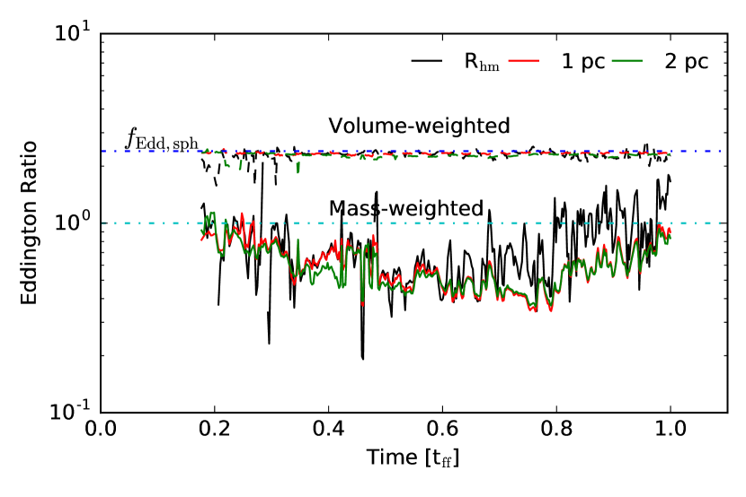
Figure 13: Evolution of the mass-weighted (solid) and volume-weighted (dashed) Eddington ratio measured from the center of the most massive cluster in the RHD run. The ratios are calculated within spheres of three radii, the cluster’s half-mass radius (black), 1 pc (red), and 2 pc (green). The blue dot-dashed line is the analytical value calculated assuming spherical symmetry. The flux-density anti-correlation reduces the mass-weighted average ratio to below unity throughout the entire simulation, while the volume-weighted value approximates the analytical estimate.

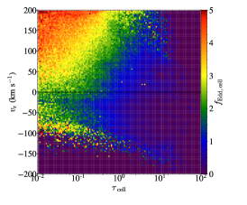
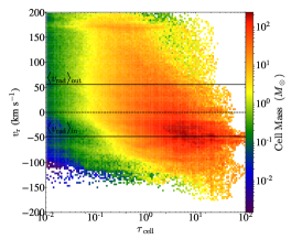
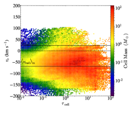
Figure 14: The mass-weighted Eddington ratio (left) and total cell mass (middle and right) shown on the cell optical depth $\tau_{\rm cell}$--radial velocity $v_{\rm rad}$ plane, all at $t=t_{\rm ff}$. The right panel is taken from the HD run. Inhomogeneity-induced matter-radiation anti-correlation is clearly visible on the left and middle panel. Super-Eddington cells accelerated by radiation to high velocities have low optical depths $\tau_{\rm cell}$. Most of the gas mass is undergoing strong gravitational infall subject to weak radiative acceleration.

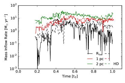
Figure 15: Evolution of the mass accretion rates across spheres of different radii around the center of the most massive cluster. Solid and dashed lines are for the RHD and HD run, respectively. Radiation pressure has minor effect on the overall accretion rates.

To quantify the mass infall, Figure 15 compares mass accretion rates across spheres centered on the most massive cluster. We compute the accretion rates by averaging the mass flux in shells

$$\dot{M}_{\rm acc}\left(R\right)=\frac{1}{N_{\rm cell}(R)}\sum_{j}\rho_{j}v_{{\rm rad},j}4\pi R^{2},$$ (38)

where $\rho_{j}$ and $v_{{\rm rad},j}$ are the density and radial velocity of cell $j$, $N_{\rm cell}(R)$ is the number of cells inside the radial shell $(R-\Delta x_{\rm min}/2,R+\Delta x_{\rm min}/2)$, and the sum is over the cells with centers located in the shell. At $R=2\,\text{pc}$, large-scale gravitational collapse channels mass toward the cluster center at high rates $\gtrsim 10\,M_{\odot}\textrm{yr}^{-1}$. Down to $R\sim\,1\,\text{pc}$, the two runs have comparable accretion rates. At the cluster’s half-mass radius the accretion rate is only slightly lower in the RHD run. These suggest that the overall dynamical influence of radiation pressure on cluster-scale gaseous collapse is minor.

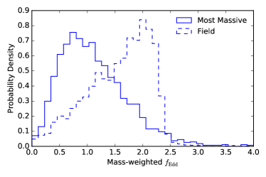
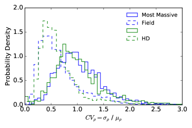
Figure 16: Left panel: Probability distribution functions of the mass-weighted Eddington ratio for isolated sink particles (dashed) and those contained in the most massive cluster (solid). To have reliable statistics, the histograms combine data from 100 time steps before $t=0.5$ $t_{\rm ff}$, which span a duration of about 0.2% $t_{\rm ff}$. It is much more likely for sinks to be under super-Eddington conditions in the field, outside any star clusters. Right panel: Probability density of the $\text{CV}_{\rho}$ for sinks in clusters (solid) and in the field (dashed). Sinks in the field, outside any star clusters, have more homogeneous local density distribution. The level of non-uniformity is independent of the presence of radiation suggesting that the density variation is driven by turbulent collapse.

Turbulent gas is organized in a network of sheets, filaments, and clumps. These structures seed the formation and merging of star clusters with a wide range of masses. Could the effects of radiation be more pronounced in more isolated regions that are forming lower-mass clusters? More homogeneous gas in shallower gravitational potential wells may be more susceptible to radiation pressure. The differential effects of radiation pressure inside and outside the most massive star cluster can be observed in the left panel of Figure 16. It compares histograms of the mass-weighted average Eddington ratio around sink particles inside the most massive cluster (solid) and in the field, both at $t=0.5\,t_{\rm ff}$ when the formation of clusters across the mass spectrum is pervasive. The average ratio is computed from cells within $r_{\rm acc}$ around each individual sink. While 57% of sinks inside the most massive clusters are super-Eddington $f_{\rm Edd}>1$, that is the case for 85% of sinks in the field regions. Next we show this trend is the result of the greater homogeneity of gas around isolated sinks.

We quantify the non-uniformity of gas around sink particles with the ‘coefficient of variation’ of gas density $\text{CV}_{\rho}=\sigma_{\rho}/\mu_{\rho}$, where $\sigma_{\rho}$ and $\mu_{\rho}$ are the standard deviation and mean of gas density within the same $r_{\rm acc}$ spheres used to construct the left panel of Figure 16. Such a local measure of density variation is appropriate because the amount of gas around individual sink is different. Alternately, we could define a coefficient of variation using the line-of-sight gas surface density by tracing rays in various directions. We computed the ray-traced coefficient and found that it correlates tightly with the density-based value.

We plot the distribution of $\text{CV}_{\rho}$ in the right panel of Figure 16. We see that the density variation both around field sinks and inside the most massive cluster is very similar between the runs, and that the density variation in the cluster is significantly higher compared to in the field. Since we expect density variation to be anti-correlated with the strength of the radiation-matter coupling, this explains the lower peak $f_{\rm Edd}$ in the cluster than in the field in the left panel of Figure 16. The result also suggests that density variation inside the cluster is mainly set by the turbulent collapse, not radiation. In the field where sinks are only beginning to form, gravity has not yet had the opportunity to disturb the local gas. Inside clusters, the hierarchical collapse has had ample time to induce inhomogeneity. The weakening of effective radiation pressure is therefore the result of such turbulent gas rearrangement.

6 Prior art and observational implications

We simulated a setup similar to that of Skinner & Ostriker (2015) but with a different radiation transport scheme and slightly different parameters. We reaffirm their main conclusion, that an anti-correlation between radiation flux and gas density reduces the forcing of IR radiation pressure on star forming gas. Our simulations, however, sample a higher total gas mass and surface density regime, one in which it may naively be expected that the radiation would more easily couple to the gas. Our simulations are initialized not from a stochastic velocity field, but are prepared via stochastic forcing. Our total gas mass and the mean surface and volume densities are factors of 10, $\sim 5$, and $\sim 2.7$ higher, respectively, than in the fiducial model of SO15. They performed radiation transport with the M1 closure, a method that does not correctly capture the directional structure of the radiation field close to point sources. Therefore they were forced to smear the point source emissivities over 1 pc spheres. Also, we perform direct gravitational force summation for sink particles, whereas SO15 spatially-smeared sink particles, with an effective softening length of 0.5 pc, onto the finite volume mesh, and solved the Poisson subsystem for the combined gas and particle density. They also used a more conservative threshold density for sink particle creation. Their simulations therefore formed substantially fewer sink particles. From an initial gas mass of $10^{6}\,M_{\odot}$, the cluster in the fiducial model of SO15 attained a final mass of $6\times 10^{5}\,M_{\odot}$ (SFE $\sim$60%) by $t\sim 3\,t_{\rm ff}$. In our simulation, where the turbulent density field reached a statistical steady state by the time gravity was switched on, the stellar mass was much larger $4.6\times 10^{6}\,M_{\odot}$ (SFE $\sim 46$%) already at $t\sim 1\,t_{\rm ff}$ and was continuously increasing.

Raskutti et al. (2016) used the same methods as SO15 but focused instead on the direct UV non-ionizing radiation pressure. They simulated the formation of star clusters at lower cloud masses $\sim 10^{5}\,M_{\odot}$ and densities $\sim 100\,M_{\odot}\,\textrm{pc}^{-2}$. As in the higher mass regime, they found that the presence of radiation pressure does limit the star formation efficiency. Furthermore, they provided an analytical upper limit on the final star formation efficiency based on the successive dispersal of high-surface density gas patches by the intensifying stellar radiation from the growing clusters. Myers et al. (2014) prepared the initial conditions by driving turbulence similar to how we did, with stochastic forcing, but their forcing was with the pure solenoidal mode and the mass of the cluster-forming cloud was much lower, $10^{3}$ $M_{\odot}$. Li et al. (2017) extended Li et al. (2015) to simulate cluster formation in magnetized clouds and with persistent stochastic forcing. They modeled both radiative and outflow feedback and were able to reproduce the local SFE of $\sim 4$%.

In contrast with these multidimensional simulations of massive cluster formation including ours, analytic and semi-analytic models assuming artificial symmetries have typically claimed radiation pressure was dominant and deleterious to star formation (Fall et al., 2010; Murray et al., 2010; Thompson et al., 2015; Kim et al., 2016). It seems clear that these divergent conclusions can be traced to the multi-dimensional nature of the turbulent clouds. Allowing for the matter-radiation anti-correlation that is ubiquitous in the cited multidimensional simulations and ours, the relative strengths of various stellar feedback processes---radiation and ionized gas pressure, stellar wind momentum, supernovae, etc.---becomes undetermined in the presently available models. Not only is the forcing of gas by radiation pressure weaker without symmetry, but the gravitational confinement of ionized gas throws into question the thermalization efficiency of stellar winds and supernovae: the winds and ejecta colliding with dense ionized gas might cool and condense on a dynamical time.

Other simulations of feedback in massive cluster formation can be found in the literature. Vázquez-Semadeni et al. (2017) simulated hierarchical collapse of filamentary structures in the collision of clouds with a total mass $\sim 10^{5}$ $M_{\odot}$ and studied feedback from photoionization heating. Howard et al. (2016, 2017) included both photoionization heating and UV direct radiation pressure to simulate cluster formation in a molecular cloud with mass $10^{6}\,M_{\odot}$, close to ours. They adopted a large initial cloud radius, 33.8 pc, and the mean density was a factor $\sim$100 lower than ours, and found that feedback was ineffective. Dale et al. (2014) included ionization heating and stellar winds and found that the dynamical impact from winds was very modest compared to photoionization. Their highest-density model had a mean density still a factor 4.2 below ours. Gavagnin et al. (2017) focused on ionization feedback and followed the collapse of a turbulent spherical cloud with mean density $\sim$14 times lower than ours. Their accurate direct gravitational force summation enabled them to study dynamical evaporation from the cluster. They found that radiative feedback limited the stellar density and this attenuated dynamical evaporation. In their simulations, the gravitational softening radius was much smaller than ours, at 0.5 $\Delta x_{\rm min}$ compared to our 2.5 $\Delta x_{\rm min}$. The details of force softening can critically influence dynamical evolution and mass segregation (Parker et al., 2015).

Observational estimates of the masses of SSCs outside the Local Group typically rely on comparing photometric colors and luminosities with spectral synthesis models (Whitmore et al., 2010; Westmoquette et al., 2014). SSCs were found to be ubiquitous in starburst and interacting galaxies. However, such estimates are subject to uncertainties in the assumed IMFs and the specific stellar evolutionary tracks. Within the Local Group, spectroscopic measurement of stellar velocity dispersions in SSCs provides a direct constraint on the cluster mass via the virial theorem. For example, in the Antennae, Mengel et al. (2002) measured velocity dispersions of $\sim 10-20\,\textrm{km}\,\textrm{s}^{-1}$ towards five clusters with sizes of 3.6--6 pc from which they deduced cluster masses of $6.5\times 10^{5}\,M_{\odot}$--$4.7\times 10^{6}\,M_{\odot}$. Larsen et al. (2004) studied a young cluster in the nearby spiral galaxy NGC 6946. A velocity dispersion of $8.8\,\textrm{km}\,\textrm{s}^{-1}$ and a radius of 10.2 pc pointed to a virial mass of $1.7\times 10^{6}\,M_{\odot}$. In the nuclear regions of M82, McCrady et al. (2005); McCrady & Graham (2007) found that the range of velocity dispersion in a dozen of SSCs implied a cluster mass range of $2\times 10^{5}\,M_{\odot}$--$4\times 10^{6}\,M_{\odot}$. The final masses of the most massive clusters in our simulations are close to the upper end of the observed range, however, the stellar velocity dispersion ($73\,\textrm{km}\,\textrm{s}^{-1}$) is considerably higher. These estimates are subject to the dependence on the internal mass distribution in the cluster that is poorly constrained in observations.

The age of our clusters 0.3 Myr is much smaller than the typical ages (6--10 Myr) of the systems observed in the optical and near-IR, yet by 6 Myr, the most massive and earliest to form stars are already lost to supernovae. With high-angular-resolution instruments such as ALMA, recently we are able to probe the massive cluster forming gas. Johnson et al. (2015) and Leroy et al. (2015) observed the star-forming clouds in the Antennae and NGC 253, respectively, and identified clouds with masses $10^{7}\,M_{\odot}$ and length scales of 30 pc. The clouds in NGC253 were further observed to have high line widths of $20-40\,\text{km}\,\text{s}^{-1}$. For direct comparison with observations, in Figure 11 we show the one-dimensional velocity dispersion $\langle v_{\rm rms}\rangle$ in the RHD run. After $\sim 0.6\,t_{\rm ff}$, the velocity dispersion becomes $\sim 50\,\text{km}\,\text{s}^{-1}$. In comparison, Turner et al. (2017) measured the CO molecular line width in the super-star-cluster-forming Cloud D1 in the dwarf galaxy NGC 5253 to be $21.7\pm 0.5\,\text{km}\,\text{s}^{-1}$. The dispersion implies a virial mass of $2.5\times 10^{5}\,M_{\odot}$ at the reference radius of 2.8 pc. When our most massive cluster grows to this mass (at $\sim$0.4 $t_{\rm ff}$), its cluster radius is 3.5 pc, and the one-dimensinoal velocity dispersion is 20.6 km s^-1, both consistent with Cloud D1. Similar to our simulations, Turner et al. (2017) also found that the molecular gas only constituted a small fraction of the global dynamical mass. These suggest that Cloud D1 could indeed be a growing massive cluster. The gas dynamics observed in our simulation supports their proposal that the star-forming molecular clumps orbit in a deep gravitational potential containing a high-mass stellar component. Furthermore, the light-to-mass ratio of Cloud D1 was estimated to be $\sim 4000$ erg s^-1 g^-1, providing observational motivation for our optimistic choice.

7 Conclusions

We have extended the IMC radiation transport scheme into a hybrid IMC-DDMC scheme that is efficient enough to permit simulating the radiation-hydrodynamics of super star cluster formation in realistic turbulent molecular clouds. We drove turbulence in $10^{7}\,M_{\odot}$ of gas and then followed gravitational collapse and subgrid star formation. The star particles organized into hierarchically merging clusters to produce a final SSC with mass $\gtrsim 10^{6}\,M_{\odot}$ and radius $\sim 1\,\textrm{pc}$. Our direct gravitational force summation in combination with the accurate hybrid radiation transport scheme we implemented allowed us to resolve gas virialization and radiative forcing in the very nucleus of the SSC.

In the course of the 0.3 Myr simulation we find that radiation pressure reduced the simulation-wide star formation efficiency by 30-35% and star formation rate by 15-50% , both relative to a radiation-free run. In contrast to previous analytical arguments that hinged on idealized geometries, we found that radiation pressure did not truncate gas infall or star formation. At the end of the simulation massive clusters continued growing at rates $\sim 1\,M_{\odot}\,\textrm{yr}^{-1}$.

Similar to Skinner & Ostriker (2015), we attribute the ineffectiveness of radiation pressure relative to 1D models to a radiation-matter anti-correlation in the turbulent cluster-forming gas. The turbulent infall enhances the density inhomogeneity in and around clusters. The gas distribution is more homogeneous around the stellar sources far from massive clusters and there the radiation accelerates gas more effectively.

The simulation produced a final peak stellar density of $\sim 10^{8}\,M_{\odot}\,\textrm{pc}^{-3}$ in an SSC with a one-dimensional stellar velocity dispersion exceeding $70$ km s^-1. These conditions favor stellar collisions and runaway merging that can produce a very massive star. We speculate that this very massive star accretes clouds condensing from the ionized gas that is gravitationally-confined in the SSC potential. If the very massive star avoids severe mass loss, such as it might embedded in the dense gaseous environment of the SSC nucleus, it can collapse directly into a massive black hole.

The hybrid IMC-DDMC particle-based radiation transport scheme is distinct from but competitive with the most advanced existing moment- or characteristics-based methods. The DDMC component of the hybrid scheme accelerates transport at high optical depths and interfaces seamlessly with the IMC scheme at low optical depths. Our implementation exploits the native parallel infrastructure of the flash hydrodynamic code to deliver excellent speedups.

References

- Abdikamalov et al. (2012) Abdikamalov E., Burrows A., Ott C. D., Löffler F., O’Connor E., Dolence J. C., Schnetter E., 2012, ApJ, 755, 111
- Allison et al. (2009) Allison R. J., Goodwin S. P., Parker R. J., Portegies Zwart S. F., de Grijs R., Kouwenhoven M. B. N., 2009, MNRAS, 395, 1449
- Andrews & Thompson (2011) Andrews B. H., Thompson T. A., 2011, ApJ, 727, 97
- Ashman & Zepf (2001) Ashman K. M., Zepf S. E., 2001, AJ, 122, 1888
- Barnes & Hut (1986) Barnes J., Hut P., 1986, Nature, 324, 446
- Bastian et al. (2014) Bastian N., Hollyhead K., Cabrera-Ziri I., 2014, MNRAS, 445, 378
- Blain et al. (2002) Blain A. W., Smail I., Ivison R. J., Kneib J.-P., Frayer D. T., 2002, Phys. Rep., 369, 111
- Casey et al. (2017) Casey C. M., et al., 2017, ApJ, 840, 101
- Chandrasekhar (1961) Chandrasekhar S., 1961, Hydrodynamic and hydromagnetic stability
- Commerçon et al. (2011) Commerçon B., Teyssier R., Audit E., Hennebelle P., Chabrier G., 2011, A&A, 529, A35
- Costa et al. (2017) Costa T., Rosdahl J., Sijacki D., Haehnelt M., 2017, preprint, (arXiv:1703.05766)
- Dale et al. (2014) Dale J. E., Ngoumou J., Ercolano B., Bonnell I. A., 2014, MNRAS, 442, 694
- Davis et al. (2014) Davis S. W., Jiang Y.-F., Stone J. M., Murray N., 2014, ApJ, 796, 107
- Densmore (2006) Densmore J. D., 2006, Annals of Nuclear Energy, 33, 343
- Densmore et al. (2007) Densmore J. D., Urbatsch T. J., Evans T. M., Buksas M. W., 2007, Journal of Computational Physics, 222, 485
- Densmore et al. (2012) Densmore J. D., Thompson K. G., Urbatsch T. J., 2012, Journal of Computational Physics, 231, 6924
- Elmegreen & Efremov (1997) Elmegreen B. G., Efremov Y. N., 1997, ApJ, 480, 235
- Ester et al. (1996) Ester M., Kriegel H.-P., Sander J., Xu X., et al., 1996, in Kdd. pp 226--231
- Fall et al. (2010) Fall S. M., Krumholz M. R., Matzner C. D., 2010, ApJ, 710, L142
- Federrath et al. (2008) Federrath C., Klessen R. S., Schmidt W., 2008, ApJ, 688, L79
- Federrath et al. (2010a) Federrath C., Roman-Duval J., Klessen R. S., Schmidt W., Mac Low M.-M., 2010a, A&A, 512, A81
- Federrath et al. (2010b) Federrath C., Banerjee R., Clark P. C., Klessen R. S., 2010b, ApJ, 713, 269
- Fleck & Canfield (1984) Fleck Jr. J. A., Canfield E. H., 1984, Journal of Computational Physics, 54, 508
- Fleck & Cummings (1971) Fleck Jr. J. A., Cummings J. D., 1971, J. Chem. Phys., 8, 313
- Fryxell et al. (2000) Fryxell B., et al., 2000, ApJS, 131, 273
- Gavagnin et al. (2017) Gavagnin E., Bleuler A., Rosdahl J., Teyssier R., 2017, MNRAS, 472, 4155
- Gentile (2001) Gentile N. A., 2001, Journal of Computational Physics, 172, 543
- Ginsburg et al. (2017) Ginsburg A., et al., 2017, ApJ, 842, 92
- Habetler & Matkowsky (1975) Habetler G. J., Matkowsky B. J., 1975, Journal of Mathematical Physics, 16, 846
- Harries (2011) Harries T. J., 2011, MNRAS, 416, 1500
- Harries (2015) Harries T. J., 2015, MNRAS, 448, 3156
- Harries et al. (2017) Harries T. J., Douglas T. A., Ali A., 2017, MNRAS, 471, 4111
- Herrera & Boulanger (2017) Herrera C. N., Boulanger F., 2017, A&A, 600, A139
- Herrera et al. (2011) Herrera C. N., Boulanger F., Nesvadba N. P. H., 2011, A&A, 534, A138
- Herrera et al. (2012) Herrera C. N., Boulanger F., Nesvadba N. P. H., Falgarone E., 2012, A&A, 538, L9
- Hollyhead et al. (2015) Hollyhead K., Bastian N., Adamo A., Silva-Villa E., Dale J., Ryon J. E., Gazak Z., 2015, MNRAS, 449, 1106
- Hopkins et al. (2010) Hopkins P. F., Murray N., Quataert E., Thompson T. A., 2010, MNRAS, 401, L19
- Howard et al. (2016) Howard C. S., Pudritz R. E., Harris W. E., 2016, MNRAS, 461, 2953
- Howard et al. (2017) Howard C. S., Pudritz R. E., Harris W. E., 2017, MNRAS, 470, 3346
- Hykes & Densmore (2009) Hykes J. M., Densmore J. D., 2009, J. Quant. Spectrosc. Radiative Transfer, 110, 1097
- Jiang et al. (2015) Jiang Y.-F., Cantiello M., Bildsten L., Quataert E., Blaes O., 2015, ApJ, 813, 74
- Johnson & Kobulnicky (2003) Johnson K. E., Kobulnicky H. A., 2003, ApJ, 597, 923
- Johnson et al. (2015) Johnson K. E., Leroy A. K., Indebetouw R., Brogan C. L., Whitmore B. C., Hibbard J., Sheth K., Evans A. S., 2015, ApJ, 806, 35
- Keady & Cleveland (2017) Keady K. P., Cleveland M. A., 2017, Journal of Computational Physics, 328, 160
- Kim et al. (2016) Kim J.-G., Kim W.-T., Ostriker E. C., 2016, ApJ, 819, 137
- Kobulnicky & Johnson (1999) Kobulnicky H. A., Johnson K. E., 1999, ApJ, 527, 154
- Kroupa (2001) Kroupa P., 2001, MNRAS, 322, 231
- Krumholz & Matzner (2009) Krumholz M. R., Matzner C. D., 2009, ApJ, 703, 1352
- Krumholz & Thompson (2012) Krumholz M. R., Thompson T. A., 2012, ApJ, 760, 155
- Krumholz & Thompson (2013) Krumholz M. R., Thompson T. A., 2013, MNRAS, 434, 2329
- Krumholz et al. (2009) Krumholz M. R., Klein R. I., McKee C. F., Offner S. S. R., Cunningham A. J., 2009, Science, 323, 754
- Kuiper et al. (2010) Kuiper R., Klahr H., Beuther H., Henning T., 2010, ApJ, 722, 1556
- Kuiper et al. (2011) Kuiper R., Klahr H., Beuther H., Henning T., 2011, ApJ, 732, 20
- Kuiper et al. (2012) Kuiper R., Klahr H., Beuther H., Henning T., 2012, A&A, 537, A122
- Larsen et al. (2004) Larsen S. S., Brodie J. P., Hunter D. A., 2004, AJ, 128, 2295
- Leitherer et al. (1999) Leitherer C., et al., 1999, ApJS, 123, 3
- Leroy et al. (2015) Leroy A. K., et al., 2015, ApJ, 801, 25
- Li et al. (2015) Li P. S., McKee C. F., Klein R. I., 2015, MNRAS, 452, 2500
- Li et al. (2017) Li P. S., Klein R. I., McKee C. F., 2017, preprint, (arXiv:1708.06770)
- Lucy (1999) Lucy L. B., 1999, A&A, 344, 282
- Maraston et al. (2004) Maraston C., Bastian N., Saglia R. P., Kissler-Patig M., Schweizer F., Goudfrooij P., 2004, A&A, 416, 467
- Maschberger & Clarke (2011) Maschberger T., Clarke C. J., 2011, MNRAS, 416, 541
- McCrady & Graham (2007) McCrady N., Graham J. R., 2007, ApJ, 663, 844
- McCrady et al. (2005) McCrady N., Graham J. R., Vacca W. D., 2005, ApJ, 621, 278
- Mengel et al. (2002) Mengel S., Lehnert M. D., Thatte N., Genzel R., 2002, A&A, 383, 137
- Moeckel & Clarke (2011) Moeckel N., Clarke C. J., 2011, MNRAS, 410, 2799
- Murray et al. (2010) Murray N., Quataert E., Thompson T. A., 2010, ApJ, 709, 191
- Myers et al. (2014) Myers A. T., Klein R. I., Krumholz M. R., McKee C. F., 2014, MNRAS, 439, 3420
- Noebauer et al. (2012) Noebauer U. M., Sim S. A., Kromer M., Röpke F. K., Hillebrandt W., 2012, MNRAS, 425, 1430
- Olczak et al. (2011) Olczak C., Spurzem R., Henning T., 2011, A&A, 532, A119
- Parker & Goodwin (2015) Parker R. J., Goodwin S. P., 2015, MNRAS, 449, 3381
- Parker et al. (2015) Parker R. J., Dale J. E., Ercolano B., 2015, MNRAS, 446, 4278
- Pollack et al. (2007) Pollack L. K., Max C. E., Schneider G., 2007, ApJ, 660, 288
- Portegies Zwart et al. (2010) Portegies Zwart S. F., McMillan S. L. W., Gieles M., 2010, ARA&A, 48, 431
- Raskutti et al. (2016) Raskutti S., Ostriker E. C., Skinner M. A., 2016, ApJ, 829, 130
- Ricker (2008) Ricker P. M., 2008, ApJS, 176, 293
- Rosdahl & Teyssier (2015) Rosdahl J., Teyssier R., 2015, MNRAS, 449, 4380
- Rosen et al. (2016) Rosen A. L., Krumholz M. R., McKee C. F., Klein R. I., 2016, MNRAS, 463, 2553
- Rosen et al. (2017) Rosen A. L., Krumholz M. R., Oishi J. S., Lee A. T., Klein R. I., 2017, Journal of Computational Physics, 330, 924
- Roth & Kasen (2015) Roth N., Kasen D., 2015, ApJS, 217, 9
- Safranek-Shrader et al. (2016) Safranek-Shrader C., Montgomery M. H., Milosavljević M., Bromm V., 2016, MNRAS, 455, 3288
- Schinnerer et al. (2008) Schinnerer E., et al., 2008, ApJ, 689, L5
- Semenov et al. (2003) Semenov D., Henning T., Helling C., Ilgner M., Sedlmayr E., 2003, A&A, 410, 611
- Skinner & Ostriker (2015) Skinner M. A., Ostriker E. C., 2015, ApJ, 809, 187
- Smith et al. (2017a) Smith A., Tsang B. T.-H., Bromm V., Milosavljevic M., 2017a, preprint, (arXiv:1709.10187)
- Smith et al. (2017b) Smith A., Bromm V., Loeb A., 2017b, MNRAS, 464, 2963
- Thompson et al. (2015) Thompson T. A., Fabian A. C., Quataert E., Murray N., 2015, MNRAS, 449, 147
- Truelove et al. (1997) Truelove J. K., Klein R. I., McKee C. F., Holliman II J. H., Howell L. H., Greenough J. A., 1997, ApJ, 489, L179
- Tsang & Milosavljević (2015) Tsang B. T.-H., Milosavljević M., 2015, MNRAS, 453, 1108
- Turk et al. (2011) Turk M. J., Smith B. D., Oishi J. S., Skory S., Skillman S. W., Abel T., Norman M. L., 2011, ApJS, 192, 9
- Turner et al. (2017) Turner J. L., Consiglio S. M., Beck S. C., Goss W. M., Ho P. T. P., Meier D. S., Silich S., Zhao J.-H., 2017, ApJ, 846, 73
- Vázquez-Semadeni et al. (2017) Vázquez-Semadeni E., González-Samaniego A., Colín P., 2017, MNRAS, 467, 1313
- Westmoquette et al. (2014) Westmoquette M. S., et al., 2014, ApJ, 789, 94
- Whitmore et al. (2010) Whitmore B. C., et al., 2010, AJ, 140, 75
- Wollaeger et al. (2013) Wollaeger R. T., van Rossum D. R., Graziani C., Couch S. M., Jordan IV G. C., Lamb D. Q., Moses G. A., 2013, ApJS, 209, 36
- Yu et al. (2017) Yu J., Puzia T. H., Lin C., Zhang Y., 2017, ApJ, 840, 91
- Zhang & Davis (2017) Zhang D., Davis S. W., 2017, ApJ, 839, 54