Primordial perturbations with pre-inflationary bounce

Yong Cai1111caiyong13@mails.ucas.ac.cn    Yu-Tong Wang1222wangyutong12@mails.ucas.ac.cn    Jin-Yun Zhao1333zhaojinyun15@mails.ucas.ac.cn    Yun-Song Piao1,2444yspiao@ucas.ac.cn 1 School of Physics, University of Chinese Academy of Sciences, Beijing 100049, China 2 Institute of Theoretical Physics, Chinese Academy of Sciences, P.O. Box 2735, Beijing 100190, China
Abstract

Based on the effective field theory (EFT) of nonsingular cosmologies, we build a stable model, without the ghost and gradient instabilities, of bounce inflation (inflation is preceded by a cosmological bounce). We perform a full simulation for the evolution of scalar perturbation, and find that the perturbation spectrum has a large-scale suppression (as expected), which is consistent with the power deficit of the cosmic microwave background (CMB) TT-spectrum at low multipoles, but unexpectedly, it also shows itself one marked lower valley, which actually provides a better fit to the dip at multipole l20similar-to𝑙20l\sim 20. The depth of valley is relevant with the physics around the bounce scale, which is model-dependent.

I Introduction

Inflation [1][2][3][4] is the current paradigm of early universe. It predicts nearly scale-invariant scalar perturbation, which is consistent with the cosmic microwave background (CMB) observations [5][6], as well as the gravitational waves (GWs). However, it is not the final story of the early universe. As pointed out by Borde, Vilenkin and Guth [7][8], inflation is past-incomplete, and “inflationary models require physics other than inflation to describe the past boundary of the inflating region of spacetime.[8].

This past-incompletion (singularity) of inflation has inspired radical alternatives to inflation, e.g., [9][10][11][12]. However, how to make the inflation happen in a past-complete scenario is also a noteworthy issue. In certain sense, this actually requires that the pre-inflationary phase should be past-complete. One possibility is that it is slow contracting, so that the infinite past is complete Minkowski spacetime. In such a scenario, a nonsingular bounce preceding inflation must occur (so-called the bounce inflation scenario) [13].

Recently, the Planck collaboration [14][15] have observed the power deficit of CMB TT-spectrum at large scale. This might be a hint of the pre-inflationary physics, which happens around 60similar-toabsent60\sim 60 efolds, e.g., [16]. The idea of bounce inflation accounted for not only the power deficit on large angular scales [13][17][18], but also a large dipole power asymmetry [17][19] in the CMB fluctuation. Thus we conjectured that the physics hinted by the CMB anomalies might be relevant with the pre-inflationary bounce, see also [20][21][22][23][24][25][26][27].

In physical time, the equation of motion of scalar perturbation ζ𝜁\zeta is

ζ¨k+(3H+Q˙sQs)ζ˙k+cs2k2a2ζk=0.subscript¨𝜁𝑘3𝐻subscript˙𝑄𝑠subscript𝑄𝑠subscript˙𝜁𝑘superscriptsubscript𝑐𝑠2superscript𝑘2superscript𝑎2subscript𝜁𝑘0\ddot{\zeta}_{k}+\left(3H+{\dot{Q}_{s}\over Q_{s}}\right)\dot{\zeta}_{k}+c_{s}^{2}{k^{2}\over a^{2}}\zeta_{k}=0\,. (1)

Generally, Qsϵcont=const.1Q_{s}\sim\epsilon_{cont}=const.\gg 1 for the contraction, while Qsϵinf<1similar-tosubscript𝑄𝑠subscriptitalic-ϵ𝑖𝑛𝑓1Q_{s}\sim\epsilon_{inf}<1 for the inflation, where ϵ=H˙/H2italic-ϵ˙𝐻superscript𝐻2\epsilon=-{\dot{H}/H^{2}}. Thus Qssubscript𝑄𝑠Q_{s} inevitably shows itself a jumping around the nonsingular bounce, even if this phase lasts shortly enough. Previous studies neglected the effect of Qssubscript𝑄𝑠Q_{s} on the perturbation spectrum, since this effect is ambiguous without a fully stable (without the ghost and gradient instabilities) nonsingular bounce. Recently, with the effective field theory (EFT) of nonsingular cosmologies [28][29][30], we have been able to stably manipulate the bounce [31][32], see also [33][34]. This impels us to reconsider the relevant issue.

In this paper, inspired by [28][29][31][32], we build a fully stable model of bounce inflation, in which initially the universe is in the ekpyrotic contraction. By numerically solving Eq. (1), we find that the pre-inflationary bounce not only brings the power deficit of the CMB TT-spectrum at low multipoles (as expected in [13][17]), but unexpectedly, also provides a better explanation to the dip at multipole l20similar-to𝑙20l\sim 20 hinted by Planck [6].

II The Lagrangian

Recently, it has been found that the nonsingular cosmological models usually suffer from the ghost or gradient instabilities (cs2<0superscriptsubscript𝑐𝑠20c_{s}^{2}<0) [35][36], see also [37][38]. Based on the EFT of nonsingular cosmologies [28][29][30], this No-go result has been clearly illustrated. The cubic Galileon interaction ϕsimilar-toabsentitalic-ϕ\sim\Box\phi in Horndeski theory [39][40][41] only moves the period of cs2<0superscriptsubscript𝑐𝑠20c_{s}^{2}<0 to the outside of bounce phase, but cannot dispels it completely [42][43]. It has been found first in [28][29] that the operator R(3)δg00superscript𝑅3𝛿superscript𝑔00R^{(3)}\delta g^{00} in EFT could play significant role in curing the gradient instability of scalar perturbation. Recently, we have built fully stable cosmological bounce models in Ref. [31] by applying the covariant LR(3)δg00subscript𝐿superscript𝑅3𝛿superscript𝑔00L_{R^{(3)}\delta g^{00}}.

We follow Ref. [31], and after defining ϕμ=μϕsubscriptitalic-ϕ𝜇subscript𝜇italic-ϕ\phi_{\mu}=\nabla_{\mu}\phi, ϕμ=μϕsuperscriptitalic-ϕ𝜇superscript𝜇italic-ϕ\phi^{\mu}=\nabla^{\mu}\phi, ϕμν=νμϕsubscriptitalic-ϕ𝜇𝜈subscript𝜈subscript𝜇italic-ϕ\phi_{\mu\nu}=\nabla_{\nu}\nabla_{\mu}\phi, X=ϕμϕμ𝑋subscriptitalic-ϕ𝜇superscriptitalic-ϕ𝜇X=\phi_{\mu}\phi^{\mu} and ϕ=ϕμμitalic-ϕsubscriptsuperscriptitalic-ϕ𝜇𝜇\Box\phi=\phi^{\mu}_{~{}\mu}, write the effective Lagrangian of nonsingular bounce inflation as (ϕitalic-ϕ\phi is set dimensionless)

Lsimilar-to𝐿absent\displaystyle L\sim Mp22RMp22XV(ϕ)superscriptsubscript𝑀𝑝22𝑅superscriptsubscript𝑀𝑝22𝑋𝑉italic-ϕ\displaystyle\underbrace{{M_{p}^{2}\over 2}R-{M_{p}^{2}\over 2}X-V(\phi)}
Contraction+InflationContractionInflation\displaystyle\text{Contraction}+\text{Inflation}
+\displaystyle+ P~(ϕ,X)+Lδg00R(3)+LδKδg00,~𝑃italic-ϕ𝑋subscript𝐿𝛿superscript𝑔00superscript𝑅3subscript𝐿𝛿𝐾𝛿superscript𝑔00\displaystyle\quad\quad\underbrace{{\tilde{P}}(\phi,X)}\quad\quad\quad\quad\quad\quad+\underbrace{L_{\delta g^{00}R^{(3)}}}\quad\quad+L_{\delta K\delta g^{00}}\,,
(Ghost free) BounceRemovingcs2<0(Ghost free) BounceRemovingsuperscriptsubscript𝑐𝑠20\displaystyle\text{(Ghost free) Bounce}\quad\quad\,\,\text{Removing}~{}c_{s}^{2}<0

where

Lδg00R(3)subscript𝐿𝛿superscript𝑔00superscript𝑅3\displaystyle L_{\delta g^{00}R^{(3)}} =\displaystyle= f1(ϕ)2δg00R(3)subscript𝑓1italic-ϕ2𝛿superscript𝑔00superscript𝑅3\displaystyle{f_{1}(\phi)\over 2}\delta g^{00}R^{(3)} (3)
=\displaystyle= f2RX2fϕϕdlnX(fϕ+fϕ2dlnX)ϕ𝑓2𝑅𝑋2subscript𝑓italic-ϕitalic-ϕ𝑑𝑋subscript𝑓italic-ϕsubscript𝑓italic-ϕ2𝑑𝑋italic-ϕ\displaystyle{f\over 2}R-{X\over 2}\int f_{\phi\phi}d\ln X-\left(f_{\phi}+\int{f_{\phi}\over 2}d\ln X\right)\Box\phi
+f2X[ϕμνϕμν(ϕ)2]f2XfXX2[ϕμϕμρϕρνϕν(ϕ)ϕμϕμνϕν],𝑓2𝑋delimited-[]subscriptitalic-ϕ𝜇𝜈superscriptitalic-ϕ𝜇𝜈superscriptitalic-ϕ2𝑓2𝑋subscript𝑓𝑋superscript𝑋2delimited-[]superscriptitalic-ϕ𝜇subscriptitalic-ϕ𝜇𝜌superscriptitalic-ϕ𝜌𝜈subscriptitalic-ϕ𝜈italic-ϕsuperscriptitalic-ϕ𝜇subscriptitalic-ϕ𝜇𝜈superscriptitalic-ϕ𝜈\displaystyle+{f\over 2X}\left[\phi_{\mu\nu}\phi^{\mu\nu}-(\Box\phi)^{2}\right]-{f-2Xf_{X}\over X^{2}}\left[\phi^{\mu}\phi_{\mu\rho}\phi^{\rho\nu}\phi_{\nu}-(\Box\phi)\phi^{\mu}\phi_{\mu\nu}\phi^{\nu}\right]\,,
LδKδg00subscript𝐿𝛿𝐾𝛿superscript𝑔00\displaystyle L_{\delta K\delta g^{00}} =\displaystyle= g1(ϕ)2δKδg00subscript𝑔1italic-ϕ2𝛿𝐾𝛿superscript𝑔00\displaystyle{g_{1}(\phi)\over 2}\delta K\delta g^{00} (4)
=\displaystyle= g21X(ϕμϕμνϕνXϕ)32gH,𝑔21𝑋superscriptitalic-ϕ𝜇subscriptitalic-ϕ𝜇𝜈superscriptitalic-ϕ𝜈𝑋italic-ϕ32𝑔𝐻\displaystyle{g\over 2}{1\over\sqrt{-X}}\left({\phi^{\mu}\phi_{\mu\nu}\phi^{\nu}\over X}-\Box\phi\right)-{3\over 2}gH\,,
f𝑓\displaystyle f =\displaystyle= f1(ϕ)[1+Xf2(ϕ)],g=g1(ϕ)[1+Xf2(ϕ)],subscript𝑓1italic-ϕdelimited-[]1𝑋subscript𝑓2italic-ϕ𝑔subscript𝑔1italic-ϕdelimited-[]1𝑋subscript𝑓2italic-ϕ\displaystyle f_{1}(\phi)\left[1+{X\over f_{2}(\phi)}\right],\quad\quad g=g_{1}(\phi)\left[1+{X\over f_{2}(\phi)}\right]\,, (5)

with f2=Xδg001=ϕ˙2(t)subscript𝑓2𝑋𝛿superscript𝑔001superscript˙italic-ϕ2𝑡f_{2}={X\over\delta g^{00}-1}={\dot{\phi}}^{2}(t), R(3)δg00superscript𝑅3𝛿superscript𝑔00R^{(3)}\delta g^{00} and δKδg00𝛿𝐾𝛿superscript𝑔00\delta K\delta g^{00} being the EFT operators (R(3)superscript𝑅3R^{(3)} is the 3-dimensional Ricci scalars on the spacelike hypersurface). We briefly review the EFT of nonsingular cosmologies in Appendix A, see (49) for the definition of δg00𝛿superscript𝑔00\delta g^{00} and δK𝛿𝐾\delta K. Though Lδg00R(3)subscript𝐿𝛿superscript𝑔00superscript𝑅3L_{\delta g^{00}R^{(3)}} has the higher order of the second order derivative of ϕitalic-ϕ\phi, it is Ostrogradski ghost-free [44][45]. Additionally, Lδg00R(3)subscript𝐿𝛿superscript𝑔00superscript𝑅3{L_{\delta g^{00}R^{(3)}}} and LδKδg00subscript𝐿𝛿𝐾𝛿superscript𝑔00L_{\delta K\delta g^{00}} do not affect the cosmological background.

III A stable model of bounce inflation

III.1 Background
Refer to caption
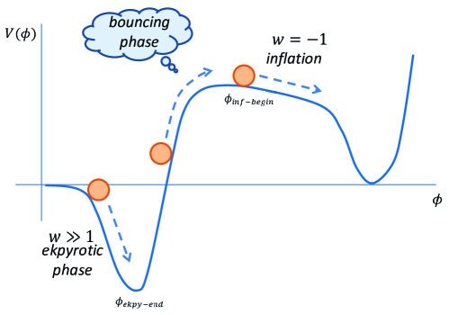
Figure 1:   A sketch of the bounce inflation scenario.

A sketch of the bounce inflation scenario is plotted in Fig. 1. We will show how to build its stable model with the Lagrangian (II).

As a specific model, we set

P~(ϕ,X)=α0(1+(ϕ/λ1)2)2Mp2X/2+β0(1+(ϕ/λ1)2)2X2/4,~𝑃italic-ϕ𝑋subscript𝛼0superscript1superscriptitalic-ϕsubscript𝜆122superscriptsubscript𝑀𝑝2𝑋2subscript𝛽0superscript1superscriptitalic-ϕsubscript𝜆122superscript𝑋24{\tilde{P}}(\phi,X)={\alpha_{0}\over\left(1+(\phi/\lambda_{1})^{2}\right)^{2}}M_{p}^{2}\,X/2+{\beta_{0}\over\left(1+(\phi/\lambda_{1})^{2}\right)^{2}}X^{2}/4, (6)
V(ϕ)=V02e2qϕ[1tanh(ϕλ2)]+Λ2(1(ϕλ3)2)2[1+tanh(ϕλ2)],𝑉italic-ϕsubscript𝑉02superscript𝑒2𝑞italic-ϕdelimited-[]1italic-ϕsubscript𝜆2Λ2superscript1superscriptitalic-ϕsubscript𝜆322delimited-[]1italic-ϕsubscript𝜆2V(\phi)=-{V_{0}\over 2}e^{\sqrt{2\over q}\phi}\left[1-\tanh\left({\phi\over\lambda_{2}}\right)\right]+{\Lambda\over 2}\left(1-\left({\phi\over\lambda_{3}}\right)^{2}\right)^{2}\left[1+\tanh\left({\phi\over\lambda_{2}}\right)\right]\,, (7)

with the positive constants λ1,2,3subscript𝜆123\lambda_{1,2,3} and q,α0,β0𝑞subscript𝛼0subscript𝛽0q,\alpha_{0},\beta_{0} being dimensionless. We have P~(ϕ,X)0~𝑃italic-ϕ𝑋0{\tilde{P}}(\phi,X)\neq 0 only around ϕ0similar-to-or-equalsitalic-ϕ0\phi\simeq 0 [46][47][48], while P~(ϕ,X)=0~𝑃italic-ϕ𝑋0{\tilde{P}}(\phi,X)=0 for |ϕ|λ1much-greater-thanitalic-ϕsubscript𝜆1|\phi|\gg\lambda_{1}.

Thus we have

3H2Mp23superscript𝐻2superscriptsubscript𝑀𝑝2\displaystyle 3H^{2}M_{p}^{2} =\displaystyle= [1α0(1+(ϕ/λ1)2)2]Mp2ϕ˙2/2+3β0(1+(ϕ/λ1)2)2ϕ˙4/4+V(ϕ),delimited-[]1subscript𝛼0superscript1superscriptitalic-ϕsubscript𝜆122superscriptsubscript𝑀𝑝2superscript˙italic-ϕ223subscript𝛽0superscript1superscriptitalic-ϕsubscript𝜆122superscript˙italic-ϕ44𝑉italic-ϕ\displaystyle\left[1-{\alpha_{0}\over\left(1+(\phi/\lambda_{1})^{2}\right)^{2}}\right]M_{p}^{2}\,\dot{\phi}^{2}/2{+{3\beta_{0}\over\left(1+(\phi/\lambda_{1})^{2}\right)^{2}}}\dot{\phi}^{4}/4+V(\phi)\,, (8)
H˙Mp2˙𝐻superscriptsubscript𝑀𝑝2\displaystyle\dot{H}M_{p}^{2} =\displaystyle= [1α0(1+(ϕ/λ1)2)2]Mp2ϕ˙2/2β0(1+(ϕ/λ1)2)2ϕ˙4/2.delimited-[]1subscript𝛼0superscript1superscriptitalic-ϕsubscript𝜆122superscriptsubscript𝑀𝑝2superscript˙italic-ϕ22subscript𝛽0superscript1superscriptitalic-ϕsubscript𝜆122superscript˙italic-ϕ42\displaystyle-\left[1-{\alpha_{0}\over\left(1+(\phi/\lambda_{1})^{2}\right)^{2}}\right]M_{p}^{2}\,\dot{\phi}^{2}/2{-{\beta_{0}\over\left(1+(\phi/\lambda_{1})^{2}\right)^{2}}\dot{\phi}^{4}/2}\,. (9)

In infinite past, the universe is almost Minkowski, which will experiences the ekpyrotic contraction. In the ekpyrotic phase (ϕλ1much-less-thanitalic-ϕsubscript𝜆1\phi\ll-\lambda_{1} and λ2subscript𝜆2-\lambda_{2}), we have P~=0~𝑃0{\tilde{P}}=0 and Vekpy=V0e2qϕsubscript𝑉𝑒𝑘𝑝𝑦subscript𝑉0superscript𝑒2𝑞italic-ϕV_{ekpy}=-V_{0}e^{\sqrt{2\over q}\phi} (q1much-less-than𝑞1q\ll 1). Thus we could write Eqs. (8) and (9) as

3H2=ϕ˙2/2V0Mp2e2qϕ,H˙=ϕ˙2/2.formulae-sequence3superscript𝐻2superscript˙italic-ϕ22subscript𝑉0superscriptsubscript𝑀𝑝2superscript𝑒2𝑞italic-ϕ˙𝐻superscript˙italic-ϕ223H^{2}=\dot{\phi}^{2}/2-{V_{0}\over M_{p}^{2}}e^{\sqrt{2\over q}\phi},\quad\quad\dot{H}=-\dot{\phi}^{2}/2. (10)

By solving (10), we have

a(t)1/ϵ,ϕ˙=2ϵ(t)1,formulae-sequencesimilar-to𝑎superscript𝑡1italic-ϵ˙italic-ϕ2italic-ϵsuperscript𝑡1a\sim(-t)^{1/\epsilon}\,,\quad\quad\dot{\phi}=\sqrt{2\over\epsilon}(-t)^{-1}\,, (11)

and

ϕ(t)=2ϵln[ϵ3ϵV0/Mp(t)1],italic-ϕ𝑡2italic-ϵitalic-ϵ3italic-ϵsubscript𝑉0subscript𝑀𝑝superscript𝑡1\phi(t)=\sqrt{2\over\epsilon}\ln\left[{\sqrt{\epsilon-3}\over\epsilon{\sqrt{V_{0}}/M_{p}}}(-t)^{-1}\right]\,, (12)

where ϵ=H˙/H2=1/q1italic-ϵ˙𝐻superscript𝐻21𝑞much-greater-than1\epsilon=-\dot{H}/H^{2}=1/q\gg 1, which suggests H=ϵ1(t)1𝐻superscriptitalic-ϵ1superscript𝑡1H=-{\epsilon}^{-1}(-t)^{-1}.

When ϕλ1similar-to-or-equalsitalic-ϕsubscript𝜆1\phi\simeq\lambda_{1}, we could have

H˙(α04β0ϕ˙24Mp21)ϕ˙2/2>0,similar-to-or-equals˙𝐻subscript𝛼04subscript𝛽0superscript˙italic-ϕ24superscriptsubscript𝑀𝑝21superscript˙italic-ϕ220\dot{H}\simeq\left({\alpha_{0}\over 4}-{\beta_{0}\dot{\phi}^{2}\over 4M_{p}^{2}}-1\right)\,\dot{\phi}^{2}/2>0\,, (13)

the nonsingular bounce will occur. While after ϕλ1,λ2much-greater-thanitalic-ϕsubscript𝜆1subscript𝜆2\phi\gg\lambda_{1},\lambda_{2}, the field ϕitalic-ϕ\phi will be canonical (P~=0~𝑃0{\tilde{P}}=0) again. We have

3H2=ϕ˙2/2+ΛMp2(1(ϕλ3)2)2,H˙=ϕ˙2/2.formulae-sequence3superscript𝐻2superscript˙italic-ϕ22Λsuperscriptsubscript𝑀𝑝2superscript1superscriptitalic-ϕsubscript𝜆322˙𝐻superscript˙italic-ϕ223H^{2}=\dot{\phi}^{2}/2+{\Lambda\over M_{p}^{2}}\left(1-\left({\phi\over\lambda_{3}}\right)^{2}\right)^{2},\quad\quad\dot{H}=-\dot{\phi}^{2}/2. (14)

Thus the slow-roll inflation will occur. Actually, after the nonsingular bounce, the Lagrangian (II) will reduce to LMp2R/2Mp2X/2Vinfsimilar-to𝐿superscriptsubscript𝑀𝑝2𝑅2superscriptsubscript𝑀𝑝2𝑋2subscript𝑉𝑖𝑛𝑓L\sim{M_{p}^{2}}R/2-{M_{p}^{2}}X/2-V_{inf} with Vinfsubscript𝑉𝑖𝑛𝑓V_{inf} being the potential of slow-roll inflation.

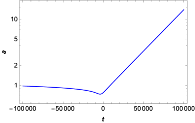
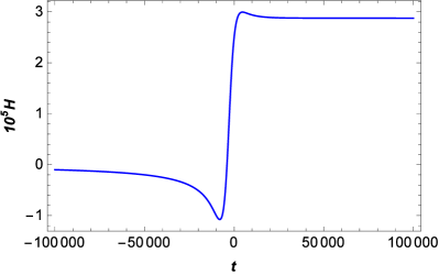
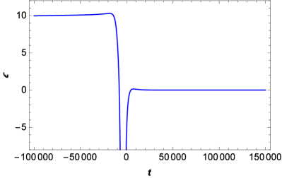
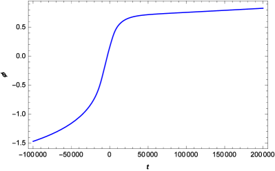
We plot the background evolution in Fig. 2 with α0=20subscript𝛼020\alpha_{0}=20, β0=5×10⁹subscript𝛽05superscript109\beta_{0}=5\times 10^{9}, λ1=0.224subscript𝜆10.224\lambda_{1}=0.224, λ2=0.0667subscript𝜆20.0667\lambda_{2}=0.0667, λ3=12subscript𝜆312\lambda_{3}=12, V0=5×10⁹Mp4subscript𝑉05superscript109superscriptsubscript𝑀𝑝4V_{0}=5\times 10^{-9}M_{p}^{4}, q=0.1𝑞0.1q=0.1, Λ=2.5×10⁹Mp4Λ2.5superscript109superscriptsubscript𝑀𝑝4\Lambda=2.5\times 10^{-9}M_{p}^{4}. The initial values are set by (11) and (12).
Refer to caption
(a)   ϕitalic-ϕ\phi
Refer to caption
(b)   a𝑎a
Refer to caption
(c)   105H/Mpsuperscript105𝐻subscript𝑀𝑝10^{5}\cdot H/M_{p}
Refer to caption
(d)   ϵ=H˙/H2italic-ϵ˙𝐻superscript𝐻2\epsilon=-\dot{H}/H^{2}
Figure 2: The background evolution of our model with α0=20subscript𝛼020\alpha_{0}=20, β0=5×10⁹subscript𝛽05superscript109\beta_{0}=5\times 10^{9}, λ1=0.224subscript𝜆10.224\lambda_{1}=0.224, λ2=0.0667subscript𝜆20.0667\lambda_{2}=0.0667, λ3=12subscript𝜆312\lambda_{3}=12, V0=5×10⁹Mp4subscript𝑉05superscript109superscriptsubscript𝑀𝑝4V_{0}=5\times 10^{-9}M_{p}^{4}, q=0.1𝑞0.1q=0.1, Λ=2.5×10⁹Mp4Λ2.5superscript109superscriptsubscript𝑀𝑝4\Lambda=2.5\times 10^{-9}M_{p}^{4}.

III.2 Simulation for the scalar perturbation spectrum

In unitary gauge δϕ=0𝛿italic-ϕ0\delta\phi=0, the quadratic action of scalar perturbation ζ𝜁\zeta for (II) is (see Appendix A and also our [28])

Sζ(2)=a3Qs(ζ˙2cs2(ζ)2a2)d4x,superscriptsubscript𝑆𝜁2superscript𝑎3subscript𝑄𝑠superscript˙𝜁2superscriptsubscript𝑐𝑠2superscript𝜁2superscript𝑎2superscript𝑑4𝑥S_{\zeta}^{(2)}=\int a^{3}Q_{s}\left(\dot{\zeta}^{2}-c_{s}^{2}{(\partial\zeta)^{2}\over a^{2}}\right)d^{4}x\,, (15)

in which

Qs=2ϕ˙4P~XXMp2H˙γ2+3(g12γMp)2,subscript𝑄𝑠2superscript˙italic-ϕ4subscript~𝑃𝑋𝑋superscriptsubscript𝑀𝑝2˙𝐻superscript𝛾23superscriptsubscript𝑔12𝛾subscript𝑀𝑝2Q_{s}={2{\dot{\phi}}^{4}{\tilde{P}}_{XX}-M_{p}^{2}{\dot{H}}\over\gamma^{2}}+{3}\left({g_{1}\over 2\gamma M_{p}}\right)^{2}, (16)
cs2Qs=c˙3aMp2,c3=aMp2γ(1+2f1Mp2),formulae-sequencesuperscriptsubscript𝑐𝑠2subscript𝑄𝑠subscript˙𝑐3𝑎superscriptsubscript𝑀𝑝2subscript𝑐3𝑎superscriptsubscript𝑀𝑝2𝛾12subscript𝑓1superscriptsubscript𝑀𝑝2c_{s}^{2}Q_{s}={{\dot{c}}_{3}\over a}-M_{p}^{2},\quad\quad c_{3}={a{M_{p}^{2}}\over\gamma}\left(1+{2f_{1}\over M_{p}^{2}}\right), (17)

with γ=H+g12Mp2𝛾𝐻subscript𝑔12superscriptsubscript𝑀𝑝2\gamma=H+{g_{1}\over 2M_{p}^{2}}.

The stabilities require Qs>0subscript𝑄𝑠0Q_{s}>0 and cs2>0superscriptsubscript𝑐𝑠20c_{s}^{2}>0. Generally, Qs>0subscript𝑄𝑠0Q_{s}>0 can be obtained by applying P~(ϕ,X)~𝑃italic-ϕ𝑋{\tilde{P}}(\phi,X). While around the bounce point H0similar-to-or-equals𝐻0H\simeq 0,

cs2γ˙(1+2f1Mp2)+2f˙1γMP2γ2.similar-tosuperscriptsubscript𝑐𝑠2˙𝛾12subscript𝑓1superscriptsubscript𝑀𝑝22subscript˙𝑓1𝛾superscriptsubscript𝑀𝑃2superscript𝛾2c_{s}^{2}\sim-{\dot{\gamma}}\left(1+{2f_{1}\over M_{p}^{2}}\right){+{2{\dot{f}}_{1}\gamma\over M_{P}^{2}}-\gamma^{2}}. (18)

We will have cs2>0superscriptsubscript𝑐𝑠20c_{s}^{2}>0 only for 2f1<Mp22subscript𝑓1superscriptsubscript𝑀𝑝22f_{1}<-{M_{p}^{2}}, as has been clarified in Refs. [28][30]. Thus the gradient instability (cs2<0superscriptsubscript𝑐𝑠20c_{s}^{2}<0) is cured by Lδg00R(3)subscript𝐿𝛿superscript𝑔00superscript𝑅3L_{\delta g^{00}R^{(3)}}, since if f10subscript𝑓10f_{1}\equiv 0, we have cs2γ˙γ2<0similar-tosuperscriptsubscript𝑐𝑠2˙𝛾superscript𝛾20c_{s}^{2}\sim-{\dot{\gamma}}-\gamma^{2}<0 around the bounce point. Here, we always could set cs2𝒪(1)similar-tosuperscriptsubscript𝑐𝑠2𝒪1c_{s}^{2}\sim{\cal O}(1) with a suitable f1(ϕ)subscript𝑓1italic-ϕf_{1}(\phi) (see also [30]) satisfying

2f1(ϕ)=γaa(Qscs2+Mp2)𝑑tMp2.2subscript𝑓1italic-ϕ𝛾𝑎𝑎subscript𝑄𝑠superscriptsubscript𝑐𝑠2superscriptsubscript𝑀𝑝2differential-d𝑡superscriptsubscript𝑀𝑝2{2f_{1}(\phi)}={\gamma\over a}\int a\left(Q_{s}c_{s}^{2}+M_{p}^{2}\right)dt-M_{p}^{2}. (19)

In conformal time η=𝑑t/a𝜂differential-d𝑡𝑎\eta=\int dt/a, the motion equation of ζ𝜁\zeta is

u′′+(cs2k2zs′′zs)u=0,superscript𝑢′′superscriptsubscript𝑐𝑠2superscript𝑘2superscriptsubscript𝑧𝑠′′subscript𝑧𝑠𝑢0\displaystyle u^{\prime\prime}+\left({c}_{s}^{2}k^{2}-{z_{s}^{\prime\prime}\over z_{s}}\right)u=0\,, (20)

where u=zsζ𝑢subscript𝑧𝑠𝜁u=z_{s}\zeta and zs=2a2Qssubscript𝑧𝑠2superscript𝑎2subscript𝑄𝑠z_{s}=\sqrt{2a^{2}Q_{s}}. In infinite past, the universe is almost Minkowski, and will come through the ekpyrotic phase. The perturbation modes have the wavelength λ1/kzs/zs′′similar-to-or-equals𝜆1𝑘much-less-thansubscript𝑧𝑠superscriptsubscript𝑧𝑠′′\lambda\simeq 1/k\ll\sqrt{z_{s}/z_{s}^{\prime\prime}} and cs2=1superscriptsubscript𝑐𝑠21c_{s}^{2}=1. Thus the initial state of the perturbation is

u12keikη.similar-to-or-equals𝑢12𝑘superscript𝑒𝑖𝑘𝜂u\simeq{1\over\sqrt{2k}}e^{-ik\eta}\,. (21)

The perturbation modes will pass through the ekpyrotic phase, the bounce phase and the inflation phase, sequentially. The resulting spectrum Pζsubscript𝑃𝜁P_{\zeta} of ζ𝜁\zeta (at kη1much-less-than𝑘𝜂1-k\eta\ll 1) is

Pζ=k32π2|ζ|2.subscript𝑃𝜁superscript𝑘32superscript𝜋2superscript𝜁2P_{\zeta}={k^{3}\over 2\pi^{2}}|\zeta|^{2}\,. (22)

In physical time, the motion equation of ζ𝜁\zeta is (1). In the ekpyrotic phase, zsa(η)1ϵekpy1similar-tosubscript𝑧𝑠𝑎similar-tosuperscript𝜂1subscriptitalic-ϵ𝑒𝑘𝑝𝑦1z_{s}\sim a\sim(-\eta)^{1\over\epsilon_{ekpy}-1}, since Qsϵekpy=const.1Q_{s}\sim\epsilon_{ekpy}=const.\gg 1. While in the inflationary phase, ϵinf<1subscriptitalic-ϵ𝑖𝑛𝑓1\epsilon_{inf}<1. This suggests that Qssubscript𝑄𝑠Q_{s} (or zsaQssimilar-tosubscript𝑧𝑠𝑎subscript𝑄𝑠z_{s}\sim a\sqrt{Q_{s}}) will show itself a jumping around the nonsingular bounce, which will inevitably affect Pζsubscript𝑃𝜁P_{\zeta}. Whether the jumping of Qssubscript𝑄𝑠Q_{s} is gentle or not is model-dependent. We will simulate its effect on Pζsubscript𝑃𝜁P_{\zeta} by numerically solving Eq. (1), with cs2=1superscriptsubscript𝑐𝑠21c_{s}^{2}=1 set by Eq.(19).

It should be mentioned that if g1=0subscript𝑔10g_{1}=0 (LδKδg00subscript𝐿𝛿𝐾𝛿superscript𝑔00L_{\delta K\delta g^{00}} is absent), we will have γ=H=0𝛾𝐻0\gamma=H=0 at the bounce point and Qs1/γ2similar-tosubscript𝑄𝑠1superscript𝛾2Q_{s}\sim 1/\gamma^{2} is divergent, see (17), so that Eq. (1) is singular. Here, in order to avoid it, we apply g1(ϕ)subscript𝑔1italic-ϕg_{1}(\phi), see also [30].

Without loss of generality, we set

Qs=𝒜Q[tanh(tt)],subscript𝑄𝑠subscript𝒜𝑄delimited-[]𝑡subscript𝑡Q_{s}={\cal A}_{Q}\left[{\cal B}-\tanh\left({t\over t_{*}}\right)\right]\,, (23)

which requires

g1(ϕ(t))=2HMp2Qs23H2Mp6Qs+Mp4(3Mp2Qs)(H˙Mp22ϕ˙4P~XX)Qs3Mp2subscript𝑔1italic-ϕ𝑡2𝐻superscriptsubscript𝑀𝑝2subscript𝑄𝑠23superscript𝐻2superscriptsubscript𝑀𝑝6subscript𝑄𝑠superscriptsubscript𝑀𝑝43superscriptsubscript𝑀𝑝2subscript𝑄𝑠˙𝐻superscriptsubscript𝑀𝑝22superscript˙italic-ϕ4subscript~𝑃𝑋𝑋subscript𝑄𝑠3superscriptsubscript𝑀𝑝2g_{1}(\phi(t))=-\frac{2HM_{p}^{2}Q_{s}-2\sqrt{3H^{2}M_{p}^{6}Q_{s}+M_{p}^{4}\left(3M_{p}^{2}-Q_{s}\right)\left(\dot{H}M_{p}^{2}-2\dot{\phi}^{4}{\tilde{P}}_{XX}\right)}}{Q_{s}-3M_{p}^{2}}\, (24)

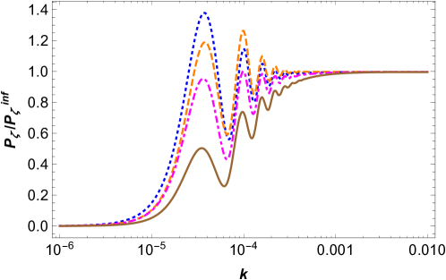
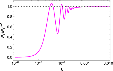
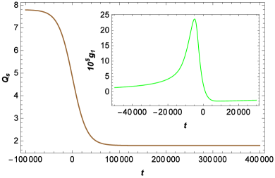
in Lagrangian (II), see (17). We plot the spectrum Pζsubscript𝑃𝜁P_{\zeta} of scalar perturbation in Fig. 3 for the background in Fig. 2 and the different values of {\cal B} and tsubscript𝑡t_{*}, where Pζinf=Hinf28Qsinfπ2Mp2(kinf)ns1superscriptsubscript𝑃𝜁𝑖𝑛𝑓superscriptsubscript𝐻𝑖𝑛𝑓28superscriptsubscript𝑄𝑠𝑖𝑛𝑓superscript𝜋2superscriptsubscript𝑀𝑝2superscript𝑘subscript𝑖𝑛𝑓subscript𝑛𝑠1P_{\zeta}^{inf}={H_{inf}^{2}\over 8Q_{s}^{inf}\pi^{2}M_{p}^{2}}\left({k\over{\cal H}_{inf}}\right)^{n_{s}-1} is that of the inflation, with Qsinfsuperscriptsubscript𝑄𝑠𝑖𝑛𝑓Q_{s}^{inf} being the value of Qssubscript𝑄𝑠Q_{s} during inflation, ns10similar-to-or-equalssubscript𝑛𝑠10n_{s}-1\simeq 0 (but is slightly red). The evolutions of Qssubscript𝑄𝑠Q_{s}, g1subscript𝑔1g_{1} and |ζ|𝜁|\zeta| with respect to t𝑡t, respectively, are plotted in Figs. 7 and 8 of Appendix B.

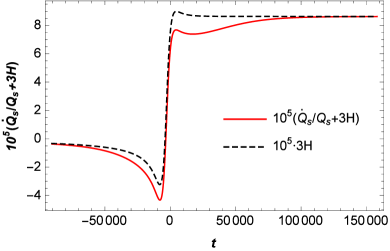
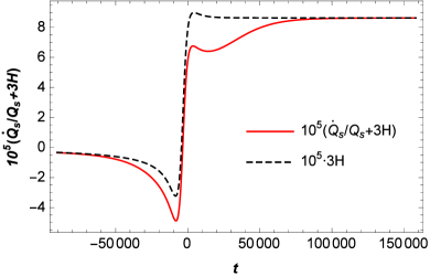
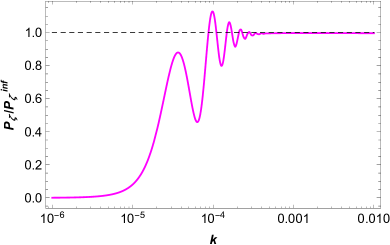
As expected in [13], Pζsubscript𝑃𝜁P_{\zeta} shows itself a large-scale cutoff, but is flat (with a damped oscillation) at small scale. However, due to the step-like evolution of Qssubscript𝑄𝑠Q_{s}, the peaks and valleys of the oscillations are obviously pulled lower. Actually, after the nonsingular bounce, with Eq. (1), we shortly have the effective Hubble parameter

Hinfeff=Hinf+Q˙s3Qs<Hinf,superscriptsubscript𝐻𝑖𝑛𝑓𝑒𝑓𝑓subscript𝐻𝑖𝑛𝑓subscript˙𝑄𝑠3subscript𝑄𝑠subscript𝐻𝑖𝑛𝑓H_{inf}^{eff}=H_{inf}+{{\dot{Q}}_{s}\over 3Q_{s}}<H_{inf}, (25)

since Q˙s<0subscript˙𝑄𝑠0{\dot{Q}}_{s}<0, see Figs. 7(b) and 8(b) in Appendix B. Thus Pζsubscript𝑃𝜁P_{\zeta} is pulled lower at the corresponding scale, since Pζ(Hinfeff)2similar-tosubscript𝑃𝜁superscriptsuperscriptsubscript𝐻𝑖𝑛𝑓𝑒𝑓𝑓2P_{\zeta}\sim(H_{inf}^{eff})^{2}. The change rate of Qssubscript𝑄𝑠Q_{s} is relevant to the physics of nonsingular bounce, as showed in Eq. (23), so the depth of valley pulled lower is actually model-dependent.

In Sec. IV.2, we will show that such a marked lower valley at corresponding scale helps to explain the dip around l20similar-to-or-equals𝑙20l\simeq 20 hinted by Planck [6].

Refer to caption
Figure 3:   Pζ/Pζinfsubscript𝑃𝜁superscriptsubscript𝑃𝜁𝑖𝑛𝑓P_{\zeta}/P_{\zeta}^{inf} with background set by Fig. 2, where the {solid brown, dotdashed magenta, dashed orange, blue dotted} curves correspond to 𝒜Q={3, 3, 3, 3}subscript𝒜𝑄3333{\cal A}_{Q}=\{3,\,3,\,3,\,3\}, ={1.3, 1.8, 2, 3}1.31.823{\cal B}=\{1.3,\,1.8,\,2,\,3\}, t={4, 4, 2.5, 4}×104subscript𝑡442.54superscript104t_{*}=\{4,\,4,\,2.5,\,4\}\times 10^{4}, respectively.

IV More on the spectrum

IV.1 Analytical estimation

We will attempt to analytically estimate Pζsubscript𝑃𝜁P_{\zeta}. The equation of motion for ζ𝜁\zeta is (20). In [26], the spectrum of primordial GWs has been calculated. Here, if the effect of Qssubscript𝑄𝑠Q_{s} is neglected, the calculation will be similar.

The bounce phase is the evolution with H˙>0˙𝐻0{\dot{H}}>0. We define that it begins and ends at ηBsubscript𝜂limit-from𝐵\eta_{B-} and ηB+subscript𝜂limit-from𝐵\eta_{B+}, respectively, at which H˙=0˙𝐻0{\dot{H}}=0. We set that H=0𝐻0H=0 at ηBsubscript𝜂𝐵\eta_{B}, which corresponds to the bounce point. Generally, ΔηB=ηB+ηB1/B+Δsubscript𝜂𝐵subscript𝜂limit-from𝐵subscript𝜂limit-from𝐵less-than-or-similar-to1subscriptlimit-from𝐵\Delta\eta_{B}=\eta_{B+}-\eta_{B-}\lesssim 1/{{\cal H}}_{B+}.

In our model (Sec. III), the contracting phase (η<ηB𝜂subscript𝜂limit-from𝐵\eta<\eta_{B-}) is ekpyrotic-like, a𝑎a is almost constant for ϵekpy1much-greater-thansubscriptitalic-ϵ𝑒𝑘𝑝𝑦1\epsilon_{ekpy}\gg 1. Considering the continuities of a𝑎a and H𝐻H at ηBsubscript𝜂limit-from𝐵\eta_{B-}, we have

a(η)=aB[x(ϵekpy1)1B1]1ϵekpy1,𝑎𝜂subscript𝑎limit-from𝐵superscriptdelimited-[]𝑥superscriptsubscriptitalic-ϵ𝑒𝑘𝑝𝑦11superscriptsubscriptlimit-from𝐵11subscriptitalic-ϵ𝑒𝑘𝑝𝑦1a(\eta)=a_{B-}\left[{x\over(\epsilon_{ekpy}-1)^{-1}{\cal H}_{B-}^{-1}}\right]^{1\over\epsilon_{ekpy}-1}, (26)

see [26] for the details, where Bsubscriptlimit-from𝐵{\cal H}_{B-} is the comoving Hubble parameter at ηBsubscript𝜂limit-from𝐵\eta_{B-} and x=ηηB+(ϵekpy1)1B1𝑥𝜂subscript𝜂limit-from𝐵superscriptsubscriptitalic-ϵ𝑒𝑘𝑝𝑦11superscriptsubscriptlimit-from𝐵1x=\eta-\eta_{B-}+(\epsilon_{ekpy}-1)^{-1}{\cal H}_{B-}^{-1}. We have zs′′/zs=a′′/asubscriptsuperscript𝑧′′𝑠subscript𝑧𝑠superscript𝑎′′𝑎z^{\prime\prime}_{s}/z_{s}=a^{\prime\prime}/a, since Qssubscript𝑄𝑠Q_{s} is constant. Thus the solution of (20) is

uk=π|x|2c1,1Hν1(1)(kx)subscript𝑢𝑘𝜋𝑥2subscript𝑐11subscriptsuperscript𝐻1subscript𝜈1𝑘𝑥u_{k}={\sqrt{\pi|x|}\over 2}c_{1,1}H^{(1)}_{\nu_{1}}(-kx) (27)

where ν1=1/2subscript𝜈112\nu_{1}=1/2 for ϵekpy1much-greater-thansubscriptitalic-ϵ𝑒𝑘𝑝𝑦1\epsilon_{ekpy}\gg 1, and the initial condition (21) has been used.

In the nonsingular bounce phase (ηB<η<ηB+subscript𝜂limit-from𝐵𝜂subscript𝜂limit-from𝐵\eta_{B-}<\eta<\eta_{B+}), H𝐻H should cross 0. We parameterize it as H=α(ttB)𝐻𝛼𝑡subscript𝑡𝐵H={\alpha}(t-t_{B}) [49] with αMP21much-less-than𝛼superscriptsubscript𝑀𝑃21{\alpha}M_{P}^{2}\ll 1. We have

aaBe12α(ttB)2aB[1+α2(ttB)2],similar-to-or-equals𝑎subscript𝑎𝐵superscript𝑒12𝛼superscript𝑡subscript𝑡𝐵2similar-to-or-equalssubscript𝑎𝐵delimited-[]1𝛼2superscript𝑡subscript𝑡𝐵2{a}\simeq{a}_{B}e^{{1\over 2}{\alpha}(t-t_{B})^{2}}\simeq{a}_{B}\left[1+{{\alpha}\over 2}(t-t_{B})^{2}\right], (28)

where a=aB𝑎subscript𝑎𝐵{a}={a}_{B} at the bouncing point t=tB𝑡subscript𝑡𝐵t=t_{B}. The continuities of a𝑎a and {\cal H} at ηBsubscript𝜂limit-from𝐵\eta_{B-} and ηB+subscript𝜂limit-from𝐵\eta_{B+} suggest B+=B+αaB2(ηB+ηB)subscriptlimit-from𝐵subscriptlimit-from𝐵𝛼superscriptsubscript𝑎𝐵2subscript𝜂limit-from𝐵subscript𝜂limit-from𝐵{{\cal H}}_{B+}={{\cal H}}_{B-}+{\alpha}{a}_{B}^{2}\left(\eta_{B+}-\eta_{B-}\right). In our models, |B|B+/4less-than-or-similar-tosubscriptlimit-from𝐵subscriptlimit-from𝐵4|{{\cal H}}_{B-}|\lesssim{{\cal H}}_{B+}/4, see Figs. 7 and 8 in Appendix B, so that we approximately have

B+αaB2ΔηB.similar-to-or-equalssubscriptlimit-from𝐵𝛼superscriptsubscript𝑎𝐵2Δsubscript𝜂𝐵{{\cal H}}_{B+}\simeq{\alpha}{a}_{B}^{2}\Delta\eta_{B}. (29)

Thus in this phase the equation (20) is

uk′′+(k2αaB2)uk=0.superscriptsubscript𝑢𝑘′′superscript𝑘2𝛼superscriptsubscript𝑎𝐵2subscript𝑢𝑘0u_{k}^{\prime\prime}+(k^{2}-{\alpha}a_{B}^{2})u_{k}=0. (30)

Its solution is

uk(η)=c2,1el(ηηB)+c2,2el(ηηB),subscript𝑢𝑘𝜂subscript𝑐21superscript𝑒𝑙𝜂subscript𝜂𝐵subscript𝑐22superscript𝑒𝑙𝜂subscript𝜂𝐵u_{k}(\eta)=c_{2,1}e^{l(\eta-\eta_{B})}+c_{2,2}e^{-l(\eta-\eta_{B})}, (31)

where l=αaB2k2𝑙𝛼superscriptsubscript𝑎𝐵2superscript𝑘2l=\sqrt{{\alpha}{a}_{B}^{2}-k^{2}}. Here, we have neglected the effect of Qssubscript𝑄𝑠Q_{s}, or it is difficult to solve Eq. (20).

In inflationary phase (ηηB+𝜂subscript𝜂limit-from𝐵\eta\geqslant\eta_{B+}), Qsinfsuperscriptsubscript𝑄𝑠𝑖𝑛𝑓Q_{s}^{inf} is almost constant. Considering the continuities of a𝑎a and \cal H at ηB+subscript𝜂limit-from𝐵\eta_{B+}, we have

ainf(η)=aB+(yB+)1ϵinf1,subscript𝑎𝑖𝑛𝑓𝜂subscript𝑎limit-from𝐵superscript𝑦subscriptlimit-from𝐵1subscriptitalic-ϵ𝑖𝑛𝑓1a_{inf}(\eta)=a_{B+}\left(-y{\cal H}_{B+}\right)^{1\over\epsilon_{inf}-1}, (32)

where y=ηηB++1/B+𝑦𝜂subscript𝜂limit-from𝐵1subscriptlimit-from𝐵y=\eta-\eta_{B+}+1/{\cal H}_{B+}, and HB+=B+/asubscript𝐻limit-from𝐵subscriptlimit-from𝐵𝑎H_{B+}={\cal H}_{B+}/a, HinfHB+less-than-or-similar-tosubscript𝐻𝑖𝑛𝑓subscript𝐻limit-from𝐵H_{inf}\lesssim H_{B+}. The solution of (20) is

uk=π|y|2[c3,1Hν2(1)(ky)+c3,2Hν2(2)(ky)]subscript𝑢𝑘𝜋𝑦2delimited-[]subscript𝑐31subscriptsuperscript𝐻1subscript𝜈2𝑘𝑦subscript𝑐32subscriptsuperscript𝐻2subscript𝜈2𝑘𝑦u_{k}={\sqrt{\pi|y|}\over 2}\left[c_{3,1}H^{(1)}_{\nu_{2}}(-ky)+c_{3,2}H^{(2)}_{\nu_{2}}(-ky)\right] (33)

where ν2=ϵinf32(ϵinf1)subscript𝜈2subscriptitalic-ϵ𝑖𝑛𝑓32subscriptitalic-ϵ𝑖𝑛𝑓1\nu_{2}={\epsilon_{inf}-3\over 2(\epsilon_{inf}-1)}.

We have Pζsubscript𝑃𝜁P_{\zeta} as

Pζ(k,B+,B,Δη)Hinf28π2QsinfMp2|c31c32|2=Pζinf|c31c32|2,subscript𝑃𝜁𝑘subscriptlimit-from𝐵subscriptlimit-from𝐵Δ𝜂superscriptsubscript𝐻𝑖𝑛𝑓28superscript𝜋2superscriptsubscript𝑄𝑠𝑖𝑛𝑓superscriptsubscript𝑀𝑝2superscriptsubscript𝑐31subscript𝑐322superscriptsubscript𝑃𝜁𝑖𝑛𝑓superscriptsubscript𝑐31subscript𝑐322P_{\zeta}(k,{\cal H}_{B+},{\cal H}_{B-},\Delta\eta)\approx\frac{H_{inf}^{2}}{8\pi^{2}Q_{s}^{inf}M_{p}^{2}}|c_{31}-c_{32}|^{2}=P_{\zeta}^{inf}|c_{31}-c_{32}|^{2}~{}, (34)

where Pζinf=Hinf28π2QsinfMp2superscriptsubscript𝑃𝜁𝑖𝑛𝑓superscriptsubscript𝐻𝑖𝑛𝑓28superscript𝜋2superscriptsubscript𝑄𝑠𝑖𝑛𝑓superscriptsubscript𝑀𝑝2P_{\zeta}^{inf}=\frac{H_{inf}^{2}}{8\pi^{2}Q_{s}^{inf}M_{p}^{2}} is that of the slow-roll inflation. Requiring the continuities of ζ𝜁\zeta and ζ˙˙𝜁\dot{\zeta}, we could write the coefficients as

(c3,1c3,2)=(3,2)×(2,1)×(c1,1c1,2),subscript𝑐31missing-subexpressionmissing-subexpressionsubscript𝑐32missing-subexpressionmissing-subexpressionsuperscript32superscript21subscript𝑐11missing-subexpressionmissing-subexpressionsubscript𝑐12missing-subexpressionmissing-subexpression\left(\begin{array}[]{ccc}c_{3,1}\\ c_{3,2}\\ \end{array}\right)={\cal{M}}^{(3,2)}\times{\cal{M}}^{(2,1)}\times\left(\begin{array}[]{ccc}c_{1,1}\\ c_{1,2}\\ \end{array}\right), (35)

see Appendix C for the matrices (2,1)superscript21{\cal{M}}^{(2,1)} and (3,2)superscript32{\cal M}^{(3,2)}.

The effects of bounce has been encoded in (3,2)superscript32{\cal M}^{(3,2)} and (2,1)superscript21{\cal M}^{(2,1)} (or |c3,1c3,2|2superscriptsubscript𝑐31subscript𝑐322|c_{3,1}-c_{3,2}|^{2}). We approximately have

|c3,1c3,2|21𝒜sin(2kB+)𝒜sin(2kB++2kΔηB)superscriptsubscript𝑐31subscript𝑐3221𝒜2𝑘subscriptlimit-from𝐵𝒜2𝑘subscriptlimit-from𝐵2𝑘Δsubscript𝜂𝐵|c_{3,1}-c_{3,2}|^{2}\approx 1-{\cal A}\sin\left({2k\over{\cal{H}}_{B+}}\right)-{\cal A}\sin\left({2k\over{\cal{H}}_{B+}}+2k\Delta\eta_{B}\right) (36)

for kB+much-greater-than𝑘subscriptlimit-from𝐵k\gg{\cal H}_{B+}, where

𝒜=B+k(1αaB22B+ΔηB)B+2k𝒜subscriptlimit-from𝐵𝑘1𝛼superscriptsubscript𝑎𝐵22subscriptlimit-from𝐵Δsubscript𝜂𝐵similar-to-or-equalssubscriptlimit-from𝐵2𝑘{\cal A}={{\cal{H}}_{B+}\over k}\left(1-{{\alpha}{a}_{B}^{2}\over 2{\cal{H}}_{B+}}\Delta\eta_{B}\right)\simeq{{\cal{H}}_{B+}\over 2k} (37)

and (29) is used, which suggests that on small scale kB+much-greater-than𝑘subscriptlimit-from𝐵k\gg{\cal H}_{B+}, Pζsubscript𝑃𝜁P_{\zeta} is flat with a rapidly damped oscillation, its maximal oscillating amplitude is around kB+similar-to-or-equals𝑘subscriptlimit-from𝐵k\simeq{\cal H}_{B+}. However, if the bounce phase lasts shortly enough, ΔηB1/B+much-less-thanΔsubscript𝜂𝐵1subscriptlimit-from𝐵\Delta\eta_{B}\ll 1/{\cal H}_{B+}, (36) will be

|c3,1c3,2|21B+ksin(2kB+).superscriptsubscript𝑐31subscript𝑐3221subscriptlimit-from𝐵𝑘2𝑘subscriptlimit-from𝐵|c_{3,1}-c_{3,2}|^{2}\approx 1-{{\cal{H}}_{B+}\over k}\sin\left({2k\over{\cal{H}}_{B+}}\right). (38)

While on large scale kB+much-less-than𝑘subscriptlimit-from𝐵k\ll{\cal H}_{B+}, Pζk2similar-tosubscript𝑃𝜁superscript𝑘2P_{\zeta}\sim k^{2} will have a strongly blue tilt, since

|c3,1c3,2|2w(ΔηB)(kB+)2superscriptsubscript𝑐31subscript𝑐322𝑤Δsubscript𝜂𝐵superscript𝑘subscriptlimit-from𝐵2|c_{3,1}-c_{3,2}|^{2}\approx w(\Delta\eta_{B})\left({k\over{\cal{H}}_{B+}}\right)^{2} (39)

where

w(ΔηB)=[(1l2ΔηB2B+)cosh(lΔηB)+l2(1B+ΔηB+l24B+ΔηB2)sinh(lΔηB)]2,𝑤Δsubscript𝜂𝐵superscriptdelimited-[]1superscript𝑙2Δsubscript𝜂𝐵2subscriptlimit-from𝐵𝑙Δsubscript𝜂𝐵𝑙21subscriptlimit-from𝐵Δsubscript𝜂𝐵superscript𝑙24subscriptlimit-from𝐵Δsuperscriptsubscript𝜂𝐵2𝑙Δsubscript𝜂𝐵2w(\Delta\eta_{B})=\left[(1-{l^{2}\Delta\eta_{B}\over 2{\cal{H}}_{B+}})\cosh(l\Delta\eta_{B})+{l\over 2}({1\over{\cal{H}}_{B+}}-\Delta\eta_{B}+{l^{2}\over 4{\cal{H}}_{B+}}\Delta\eta_{B}^{2})\sinh(l\Delta\eta_{B})\right]^{2}, (40)

which is w(ΔηB)1similar-to-or-equals𝑤Δsubscript𝜂𝐵1w(\Delta\eta_{B})\simeq 1 for ΔηB0similar-to-or-equalsΔsubscript𝜂𝐵0\Delta\eta_{B}\simeq 0.

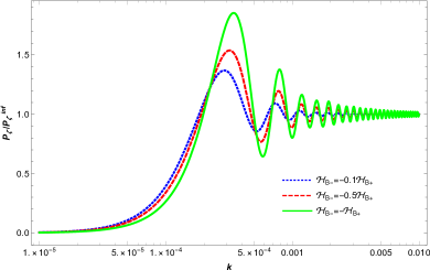
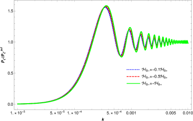
We plot Pζsubscript𝑃𝜁P_{\zeta} for (34) in Figs. 4 for the different values of ΔηΔ𝜂\Delta\eta and Bsubscriptlimit-from𝐵{\cal H}_{B-}. We see that for k>B+𝑘subscriptlimit-from𝐵k>{\cal H}_{B+}, Pζk0similar-tosubscript𝑃𝜁superscript𝑘0P_{\zeta}\sim k^{0} but has a damped oscillation, while for k<B+𝑘subscriptlimit-from𝐵k<{\cal H}_{B+}, Pζk2similar-tosubscript𝑃𝜁superscript𝑘2P_{\zeta}\sim k^{2} shows itself a large-scale cutoff. Thus (34) is consistent with our simulation result (see Fig. 7 in Sec. III) well at large and small scales, respectively.

However, since we have neglected the step-like evolution of Qssubscript𝑄𝑠Q_{s}, the pull-lower around kB+similar-to-or-equals𝑘subscriptlimit-from𝐵k\simeq{\cal H}_{B+} in Fig. 7(d) cannot be reflected in (34).
Refer to caption
(a)   Δη=0.1/B+Δ𝜂0.1subscriptlimit-from𝐵\Delta\eta=0.1/{{\cal{H}}_{B+}}
Refer to caption
(b)   Δη=0.5/B+Δ𝜂0.5subscriptlimit-from𝐵\Delta\eta=0.5/{{\cal{H}}_{B+}}
Figure 4: The power spectrum with different ΔηΔ𝜂\Delta\eta and different B/B+subscriptlimit-from𝐵subscriptlimit-from𝐵{{\cal H}_{B-}/{\cal H}_{B+}}.

IV.2 Template

To conveniently fit the observation data, a simple “Template” capturing the essential shape of Pζsubscript𝑃𝜁P_{\zeta} is indispensable. Based on the simulation in Sec. III and the analytical estimate in Sec. IV.1, we write it as

Pζ=F(k,B+,Ad,ωd)Pζinf,subscript𝑃𝜁𝐹𝑘subscriptlimit-from𝐵subscript𝐴𝑑subscript𝜔𝑑subscriptsuperscript𝑃𝑖𝑛𝑓𝜁P_{\zeta}=F(k,{\cal H}_{B+},A_{d},\omega_{d})\cdot P^{inf}_{\zeta}\,, (41)

where Pζinf=Ainf(kk)ninf1superscriptsubscript𝑃𝜁𝑖𝑛𝑓subscript𝐴𝑖𝑛𝑓superscript𝑘subscript𝑘subscript𝑛𝑖𝑛𝑓1P_{\zeta}^{inf}=A_{inf}({k\over k_{*}})^{n_{inf}-1} is the spectrum predicted by slow-roll inflation, and Ainfsubscript𝐴𝑖𝑛𝑓A_{inf} is the amplitude at the pivot scale ksubscript𝑘k_{*}, ninfsubscript𝑛𝑖𝑛𝑓n_{inf} is its tilt, and

F(k,B+,Ad,ωd)𝐹𝑘subscriptlimit-from𝐵subscript𝐴𝑑subscript𝜔𝑑\displaystyle F(k,{\cal H}_{B+},A_{d},\omega_{d}) =\displaystyle= {1+e(k/B+)2(kB+)2\displaystyle\Big{\{}1+e^{-(k/{\cal H}_{B+})^{2}}\left({k\over{\cal H}_{B+}}\right)^{2} (42)
+e(k/B+)2sin(2k/B+)k/B+}[1Adeωd(kB+π)2].\displaystyle+e^{-(k/{\cal H}_{B+})^{2}}-{\sin(2k/{\cal H}_{B+})\over k/{\cal H}_{B+}}\Big{\}}\cdot\left[1-A_{d}\cdot e^{-\omega_{d}({k\over{\cal H}_{B+}}-\pi)^{2}}\right]\,.

Here, the parameters set (B+,Ad,ωd)subscriptlimit-from𝐵subscript𝐴𝑑subscript𝜔𝑑({\cal H}_{B+},A_{d},\omega_{d}) reflects the effect of pre-inflationary bounce on the spectrum. Around kB+greater-than-or-equivalent-to𝑘subscriptlimit-from𝐵{k\gtrsim{\cal H}_{B+}}, we have

F(k,B+,Ad,ωd)1Ade𝒪(1)ωd,similar-to-or-equals𝐹𝑘subscriptlimit-from𝐵subscript𝐴𝑑subscript𝜔𝑑1subscript𝐴𝑑superscript𝑒𝒪1subscript𝜔𝑑F(k,{\cal H}_{B+},A_{d},\omega_{d})\simeq 1-A_{d}\,e^{-{\cal O}(1)\omega_{d}}, (43)

so Adsubscript𝐴𝑑A_{d} and ωdsubscript𝜔𝑑\omega_{d} (related with the parameter Δη<1/B+Δ𝜂1subscriptlimit-from𝐵\Delta\eta<1/{\cal H}_{B+} in Sec. IV.1) depict the width and depth of valley around kHB+greater-than-or-equivalent-to𝑘subscript𝐻limit-from𝐵k\gtrsim H_{B+}, respectively. Here, Adsubscript𝐴𝑑A_{d} is related with the change rate of Qssubscript𝑄𝑠Q_{s} (neglected in Sec. IV.1). With Eq. (25), we have approximately

Ad2|Q˙s|max3HinfQssimilar-to-or-equalssubscript𝐴𝑑2subscriptsubscript˙𝑄𝑠𝑚𝑎𝑥3subscript𝐻𝑖𝑛𝑓subscript𝑄𝑠A_{d}\simeq{2\left|{\dot{Q}}_{s}\right|_{max}\over 3H_{inf}Q_{s}} (44)

noting Q˙s<0subscript˙𝑄𝑠0{\dot{Q}}_{s}<0. In (42), we have

F(k,B+,Ad,ωd)1sin(2k/B+)k/B+similar-to𝐹𝑘subscriptlimit-from𝐵subscript𝐴𝑑subscript𝜔𝑑12𝑘subscriptlimit-from𝐵𝑘subscriptlimit-from𝐵F(k,{\cal H}_{B+},A_{d},\omega_{d})\sim 1-{\sin(2k/{\cal H}_{B+})\over k/{\cal H}_{B+}} (45)

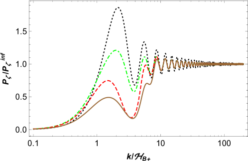
for kB+much-greater-than𝑘subscriptlimit-from𝐵k\gg{\cal H}_{B+}, which equals to (38), while for kB+much-less-than𝑘subscriptlimit-from𝐵k\ll{\cal H}_{B+}, we approximately have F(k,B+,Ad,ωd)(kB+)2similar-to-or-equals𝐹𝑘subscriptlimit-from𝐵subscript𝐴𝑑subscript𝜔𝑑superscript𝑘subscriptlimit-from𝐵2F(k,{\cal H}_{B+},A_{d},\omega_{d})\simeq({k\over{\cal H}_{B+}})^{2}, which is consistent with (39). Pζsubscript𝑃𝜁P_{\zeta} for the “Template” (42) is plotted in Fig. 5. We see that (42) has effectively captured the essential shape of Pζsubscript𝑃𝜁P_{\zeta} showed in Fig. 3.

IV.3 Data fitting

We modified the CAMB and CosmoMC code package and perform a global fitting with Planck2015 data. The parameter set of the lensed-ΛΛ\LambdaCDM model is {Ωbh2,Ωch2,100θMC,τ,ln(1010Ainf),ninf}subscriptΩ𝑏superscript2subscriptΩ𝑐superscript2100subscript𝜃MC𝜏superscript1010subscript𝐴𝑖𝑛𝑓subscript𝑛𝑖𝑛𝑓\{\Omega_{b}h^{2},\Omega_{c}h^{2},100\theta_{\mathrm{MC}},\tau,\ln(10^{10}A_{inf}),n_{inf}\}, with Ωbh2subscriptΩ𝑏superscript2\Omega_{b}h^{2} the baryon density, Ωch2subscriptΩ𝑐superscript2\Omega_{c}h^{2} the cold dark matter density, θMCsubscript𝜃MC\theta_{\mathrm{MC}} the angular size of the sound horizon at decoupling, and τ𝜏\tau the reionization optical depth. We also include the parameters set {B+,Ad,ωd}subscriptlimit-from𝐵subscript𝐴𝑑subscript𝜔𝑑\{{\cal H}_{B+},A_{d},\omega_{d}\} (so-called the bounce 3-parameters) defined in (42), which captures the physics of pre-inflationary bounce, as has been argued. We set the pivot scale k=0.05Mpc1subscript𝑘0.05𝑀𝑝superscript𝑐1k_{*}=0.05Mpc^{-1}, roughly in the middle of the logarithmic range of scales probed by Planck.

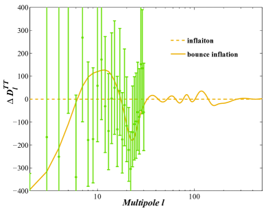
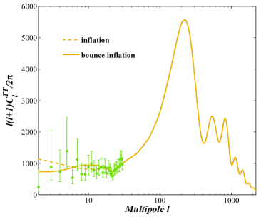
With (42), we plot the CMB TT-spectrum DlTTl(l+1)ClTT/2πsuperscriptsubscript𝐷𝑙𝑇𝑇𝑙𝑙1superscriptsubscript𝐶𝑙𝑇𝑇2𝜋D_{l}^{TT}\equiv l(l+1)C_{l}^{TT}/2\pi and ΔDlTTΔsuperscriptsubscript𝐷𝑙𝑇𝑇\Delta D_{l}^{TT} in Fig. 6 with the best-fit parameters set {Ωbh2,Ωch2,100θMC,τ,ln(1010Ainf),ninf,B+,Ad,ωd}subscriptΩ𝑏superscript2subscriptΩ𝑐superscript2100subscript𝜃MC𝜏superscript1010subscript𝐴𝑖𝑛𝑓subscript𝑛𝑖𝑛𝑓subscriptlimit-from𝐵subscript𝐴𝑑subscript𝜔𝑑\{\Omega_{b}h^{2},\Omega_{c}h^{2},100\theta_{\mathrm{MC}},\tau,\ln(10^{10}A_{inf}),n_{inf},{\cal H}_{B+},A_{d},\omega_{d}\}. Since WMAP and Planck, some models attempting to explain the anomalies of CMB at large scale (but not solving the initial singularity) have been proposed [50][51][52][53][54][55]. We see that the spectrum (42) of scalar perturbation predicted by our model could fit better not only the power deficit of the CMB TT-spectrum at low multipoles, but also the dip at l20similar-to𝑙20l\sim 20. Actually, after we add the bounce 3-parameters {B+,Ad,ωd}subscriptlimit-from𝐵subscript𝐴𝑑subscript𝜔𝑑\{{\cal H}_{B+},A_{d},\omega_{d}\} into the parameter set of the ΛΛ\LambdaCDM model, the corresponding Δχ2Δsuperscript𝜒2\Delta\chi^{2} value can be greatly improved. The details will be presented in upcoming work.

V Conclusion

In bounce inflation scenario, the inflation is singularity-free (past-complete). However, its pathology-free model has been still lacking. Here, we showed such a model. The nonsingular bounce is implemented by applying P~(ϕ,X)~𝑃italic-ϕ𝑋{\tilde{P}}(\phi,X), see (6), which is ghost-free, while cs2<0superscriptsubscript𝑐𝑠20c_{s}^{2}<0 is dispelled by Lδg00R(3)subscript𝐿𝛿superscript𝑔00superscript𝑅3L_{\delta g^{00}R^{(3)}} [31].

We perform a full simulation for the evolution of scalar perturbation, and find that the spectrum Pζsubscript𝑃𝜁P_{\zeta} has a suppression at large scale kB+much-less-than𝑘subscriptlimit-from𝐵k\ll{\cal H}_{B+} but is flat (with a damped oscillation) at small scale kB+much-greater-than𝑘subscriptlimit-from𝐵k\gg{\cal H}_{B+}, which confirms the earlier results showed in [13][17] and is consistent with the power deficit of the CMB TT-spectrum at low multipoles l30less-than-or-similar-to𝑙30l\lesssim 30; but unexpectedly, Pζsubscript𝑃𝜁P_{\zeta} also shows itself one marked lower valley at kB+greater-than-or-equivalent-to𝑘subscriptlimit-from𝐵k\gtrsim{\cal H}_{B+}, though the depth is model-dependent. We show that this lower valley actually provides a better fit to the dip at l20similar-to𝑙20l\sim 20 hinted by Planck [6]. Based on the simulation and the analytical estimation for the perturbation spectrum, we also offer a “Template” of Pζsubscript𝑃𝜁P_{\zeta} (effectively capturing the physics of bounce) to fit data.

The equation of motion of GWs mode γijsubscript𝛾𝑖𝑗\gamma_{ij} for (II) is

γ¨k+(3H+Q˙TQT)γ˙k+cT2k2a2γk=0,subscript¨𝛾𝑘3𝐻subscript˙𝑄𝑇subscript𝑄𝑇subscript˙𝛾𝑘superscriptsubscript𝑐𝑇2superscript𝑘2superscript𝑎2subscript𝛾𝑘0\ddot{\gamma}_{k}+\left(3H+{{\dot{Q}}_{T}\over Q_{T}}\right)\dot{\gamma}_{k}+c_{T}^{2}{k^{2}\over a^{2}}\gamma_{k}=0\,, (46)

which is unaffected by the operators R(3)δg00superscript𝑅3𝛿superscript𝑔00R^{(3)}\delta g^{00} and δKδg00𝛿𝐾𝛿superscript𝑔00\delta K\delta g^{00}, where QT=Mp2subscript𝑄𝑇superscriptsubscript𝑀𝑝2Q_{T}=M_{p}^{2}. We plot the primordial GWs spectrum PTsubscript𝑃𝑇P_{T} in Fig. 5 (the black dot curve) with PTinf=2Hinf2π2Mp2superscriptsubscript𝑃𝑇𝑖𝑛𝑓2superscriptsubscript𝐻𝑖𝑛𝑓2superscript𝜋2superscriptsubscript𝑀𝑝2P_{T}^{inf}={2H_{inf}^{2}\over\pi^{2}M_{p}^{2}}, see also [26]. It should be mentioned that if QTMp2subscript𝑄𝑇superscriptsubscript𝑀𝑝2Q_{T}\neq M_{p}^{2} around the nonsingular bounce (the gravity is modified completely), PTsubscript𝑃𝑇P_{T} will be different. It is also possible that the corresponding gravity has a large parity violation [56], which might be imprinted in CMB.

Our work highlight the conjecture again that the physics hinted by the large-scale anomalies of CMB is related with the pre-inflationary bounce. The nonsingular cosmological bounce also has been implemented in some models of modified gravity [57, 58, 59, 60, 61, 62, 63, 64, 65, 66, 67, 68], see also [69][70] for reviews. Confronting the corresponding models with the CMB data will be interesting.
Refer to caption
Figure 5: The black dotted curve is the spectrum PT/PTinfsubscript𝑃𝑇superscriptsubscript𝑃𝑇𝑖𝑛𝑓P_{T}/P_{T}^{inf} of the primordial GWs in bounce inflation scenario, see [26], while the {green dotdashed, red dashed, brown solid} curves are those of the primordial scalar perturbation based on the results of “Template” (42) with Ad={0.25, 0.8, 0.8}subscript𝐴𝑑0.250.80.8A_{d}=\{0.25,\,0.8,\,0.8\}, d={π,π,π}𝑑𝜋𝜋𝜋d=\{\pi,\,\pi,\,\pi\} and ωd={0.25, 0.25, 0.1}subscript𝜔𝑑0.250.250.1\omega_{d}=\{0.25,\,0.25,\,0.1\}, which are consistent with those in Fig. 3.
Refer to caption
(a)   l(l+1)ClTT/2π𝑙𝑙1superscriptsubscript𝐶𝑙𝑇𝑇2𝜋l(l+1)C_{l}^{TT}/2\pi
Refer to caption
(b)   ΔDlTTΔsuperscriptsubscript𝐷𝑙𝑇𝑇\Delta D_{l}^{TT}
Figure 6: The green points show the Planck2015 data with 1σ1𝜎1\sigma errors. The best-fit values of parameters are ln(1010Ainf)superscript1010subscript𝐴𝑖𝑛𝑓\ln(10^{10}A_{inf}) = 3.091, ninfsubscript𝑛𝑖𝑛𝑓n_{inf} = 0.966, ln(B+)=7.51subscriptlimit-from𝐵7.51\ln({\cal H}_{B+})=-7.51, Ad=0.87subscript𝐴𝑑0.87A_{d}=0.87, ωd=5.47subscript𝜔𝑑5.47\omega_{d}=5.47.

Acknowledgments

YC would like to thank Youping Wan and Yi-Fu Cai for discussions and hospitalities during his visit at University of Science and Technology of China. YSP thanks Mingzhe Li for helpful suggestions in USTC-ICTS seminar. We acknowledge the use of CAMB and CosmoMC. This work is supported by NSFC, No. 11575188, 11690021, and also supported by the Strategic Priority Research Program of CAS, No. XDA04075000, XDB23010100.

Appendix A The EFT of nonsingular cosmologies

In this Appendix, we briefly review the EFT of nonsingular cosmologies, see [28] for the details.

With the ADM 3+1313+1 decomposition, we have

gμν=(NkNkN2NjNihij),gμν=(N2NjN2NiN2hijNiNjN2),formulae-sequencesubscript𝑔𝜇𝜈subscript𝑁𝑘superscript𝑁𝑘superscript𝑁2subscript𝑁𝑗subscript𝑁𝑖subscript𝑖𝑗superscript𝑔𝜇𝜈superscript𝑁2superscript𝑁𝑗superscript𝑁2superscript𝑁𝑖superscript𝑁2superscript𝑖𝑗superscript𝑁𝑖superscript𝑁𝑗superscript𝑁2g_{\mu\nu}=\left(\begin{array}[]{cc}N_{k}N^{k}-N^{2}&N_{j}\\ N_{i}&h_{ij}\\ \end{array}\right)\,,\qquad g^{\mu\nu}=\left(\begin{array}[]{cc}-N^{-2}&{N^{j}\over N^{2}}\\ {N^{i}\over N^{2}}&h^{ij}-{N^{i}N^{j}\over N^{2}}\\ \end{array}\right)\,,\qquad (47)

and g=Nh𝑔𝑁\sqrt{-g}=N\sqrt{h}, where Ni=hijNjsubscript𝑁𝑖subscript𝑖𝑗superscript𝑁𝑗N_{i}=h_{ij}N^{j}. The induced metric on 3-dimensional hypersurface is hμν=gμν+nμnνsubscript𝜇𝜈subscript𝑔𝜇𝜈subscript𝑛𝜇subscript𝑛𝜈h_{\mu\nu}=g_{\mu\nu}+n_{\mu}n_{\nu}, where nμ=n0(dt/dxμ)=(N,0,0,0)subscript𝑛𝜇subscript𝑛0𝑑𝑡𝑑superscript𝑥𝜇𝑁000n_{\mu}=n_{0}(dt/dx^{\mu})=(-N,0,0,0), nν=gμνnμ=(1/N,Ni/N)superscript𝑛𝜈superscript𝑔𝜇𝜈subscript𝑛𝜇1𝑁superscript𝑁𝑖𝑁n^{\nu}=g^{\mu\nu}n_{\mu}=({1/N},-{N^{i}/N}) is orthogonal to the spacelike hypersurface, and nμnμ=1subscript𝑛𝜇superscript𝑛𝜇1n_{\mu}n^{\mu}=-1. Thus

hμν=(NkNkNjNihij),hμν=(000hij).formulae-sequencesubscript𝜇𝜈subscript𝑁𝑘superscript𝑁𝑘subscript𝑁𝑗subscript𝑁𝑖subscript𝑖𝑗superscript𝜇𝜈000superscript𝑖𝑗h_{\mu\nu}=\left(\begin{array}[]{cc}N_{k}N^{k}&N_{j}\\ N_{i}&h_{ij}\\ \end{array}\right)\,,\qquad h^{\mu\nu}=\left(\begin{array}[]{cc}0&0\\ 0&h^{ij}\\ \end{array}\right)\,.\qquad (48)

The EFT is [28]

S𝑆\displaystyle S =\displaystyle= d4xg[Mp22f(t)RΛ(t)c(t)g00\displaystyle\int d^{4}x\sqrt{-g}\Big{[}{M_{p}^{2}\over 2}f(t)R-\Lambda(t)-c(t)g^{00} (49)
+M24(t)2(δg00)2m33(t)2δKδg00m42(t)(δK2δKμνδKμν)+m~42(t)2R(3)δg00superscriptsubscript𝑀24𝑡2superscript𝛿superscript𝑔002superscriptsubscript𝑚33𝑡2𝛿𝐾𝛿superscript𝑔00superscriptsubscript𝑚42𝑡𝛿superscript𝐾2𝛿subscript𝐾𝜇𝜈𝛿superscript𝐾𝜇𝜈superscriptsubscript~𝑚42𝑡2superscript𝑅3𝛿superscript𝑔00\displaystyle+{M_{2}^{4}(t)\over 2}(\delta g^{00})^{2}-{m_{3}^{3}(t)\over 2}\delta K\delta g^{00}-m_{4}^{2}(t)\left(\delta K^{2}-\delta K_{\mu\nu}\delta K^{\mu\nu}\right)+{\tilde{m}_{4}^{2}(t)\over 2}R^{(3)}\delta g^{00}
m¯42(t)δK2+m¯5(t)2R(3)δK+λ¯(t)2(R(3))2+superscriptsubscript¯𝑚42𝑡𝛿superscript𝐾2subscript¯𝑚5𝑡2superscript𝑅3𝛿𝐾¯𝜆𝑡2superscriptsuperscript𝑅32\displaystyle-\bar{m}_{4}^{2}(t)\delta K^{2}+{\bar{m}_{5}(t)\over 2}R^{(3)}\delta K+{\bar{\lambda}(t)\over 2}(R^{(3)})^{2}+...
λ~(t)Mp2iR(3)iR(3)+],\displaystyle-{\tilde{\lambda}(t)\over M_{p}^{2}}\nabla_{i}R^{(3)}\nabla^{i}R^{(3)}+...\Big{]}\,,

where δg00=g00+1𝛿superscript𝑔00superscript𝑔001\delta g^{00}=g^{00}+1, R(3)superscript𝑅3R^{(3)} is the 3-dimensional Ricci scalar, Kμν=hμσσnνsubscript𝐾𝜇𝜈superscriptsubscript𝜇𝜎subscript𝜎subscript𝑛𝜈K_{\mu\nu}=h_{\mu}^{\sigma}\nabla_{\sigma}n_{\nu} is the extrinsic curvature, δKμν=KμνhμνH𝛿subscript𝐾𝜇𝜈subscript𝐾𝜇𝜈subscript𝜇𝜈𝐻\delta K_{\mu\nu}=K_{\mu\nu}-h_{\mu\nu}H.

Here, we focus on building a stable model of bounce inflation. We only consider the coefficients set (f,c,Λ,M2,m3,m~4)𝑓𝑐Λsubscript𝑀2subscript𝑚3subscript~𝑚4(f,c,\Lambda,M_{2},m_{3},{\tilde{m}}_{4}), and set other coefficients in (49) equal to 0. We always could set f=1𝑓1f=1, which suggests c(t)=Mp2H˙𝑐𝑡superscriptsubscript𝑀𝑝2˙𝐻c(t)=-M_{p}^{2}{\dot{H}} and c(t)+Λ(t)=3Mp2H2𝑐𝑡Λ𝑡3superscriptsubscript𝑀𝑝2superscript𝐻2c(t)+\Lambda(t)=3M_{p}^{2}H^{2}.

As pointed out in Ref. [33], the R(3)δKsuperscript𝑅3𝛿𝐾R^{(3)}\delta K operator in EFT could play similar role as R(3)δg00superscript𝑅3𝛿superscript𝑔00R^{(3)}\delta g^{00}, which we will consider elsewhere. Mapping (II) into the EFT (49), we have M24(t)=X2P~XXsuperscriptsubscript𝑀24𝑡superscript𝑋2subscript~𝑃𝑋𝑋M_{2}^{4}(t)=X^{2}{\tilde{P}}_{XX}, m33(t)=g1(ϕ)superscriptsubscript𝑚33𝑡subscript𝑔1italic-ϕm_{3}^{3}(t)=-g_{1}(\phi) and m~42=f1(ϕ)superscriptsubscript~𝑚42subscript𝑓1italic-ϕ\tilde{m}_{4}^{2}=f_{1}(\phi). Only with (M2,m3,m~4)0subscript𝑀2subscript𝑚3subscript~𝑚40(M_{2},m_{3},{\tilde{m}}_{4})\neq 0, the quadratic action of scalar perturbation ζ𝜁\zeta is (see, e.g., our [28])

Sζ(2)=d4xa3Qs(ζ˙2cs2(ζ)2a2),subscriptsuperscript𝑆2𝜁superscript𝑑4𝑥superscript𝑎3subscript𝑄𝑠superscript˙𝜁2superscriptsubscript𝑐𝑠2superscript𝜁2superscript𝑎2\displaystyle S^{(2)}_{\zeta}=\int d^{4}x\,a^{3}Q_{s}\left(\dot{\zeta}^{2}-c_{s}^{2}{(\partial\zeta)^{2}\over a^{2}}\right)\,, (50)

where

Qs=2M24γ2+3m364Mp2γ2H˙Mp2γ2,subscript𝑄𝑠2superscriptsubscript𝑀24superscript𝛾23superscriptsubscript𝑚364superscriptsubscript𝑀𝑝2superscript𝛾2˙𝐻superscriptsubscript𝑀𝑝2superscript𝛾2\displaystyle Q_{s}=\frac{2M_{2}^{4}}{\gamma^{2}}+\frac{3m_{3}^{6}}{4M_{p}^{2}{\gamma^{2}}}-\frac{\dot{H}M_{p}^{2}}{\gamma^{2}}\,, (51)
cs2Qs=c˙3aMp2subscriptsuperscript𝑐2𝑠subscript𝑄𝑠subscript˙𝑐3𝑎superscriptsubscript𝑀𝑝2\displaystyle c^{2}_{s}Q_{s}={\dot{c}_{3}\over a}-M_{p}^{2}\, (52)
c3=aMp2γ(1+2m~42Mp2),subscript𝑐3𝑎superscriptsubscript𝑀𝑝2𝛾12superscriptsubscript~𝑚42superscriptsubscript𝑀𝑝2\displaystyle c_{3}=\frac{aM_{p}^{2}}{\gamma}\left(1+{2{\tilde{m}}_{4}^{2}\over M_{p}^{2}}\right)\,, (53)

where γ=Hm33/(2Mp2)𝛾𝐻superscriptsubscript𝑚332superscriptsubscript𝑀𝑝2\gamma=H-{m_{3}^{3}/(2M_{p}^{2})}. Only if Qs>0subscript𝑄𝑠0Q_{s}>0 and cs2>0superscriptsubscript𝑐𝑠20c_{s}^{2}>0, the nonsingular cosmological model is healthy. In models with the operator (δg00)2superscript𝛿superscript𝑔002(\delta g^{00})^{2}, Qs>0subscript𝑄𝑠0Q_{s}>0 always can be obtained, since (δg00)2superscript𝛿superscript𝑔002(\delta g^{00})^{2} contributes ζ˙2superscript˙𝜁2{\dot{\zeta}}^{2}. While cs2>0superscriptsubscript𝑐𝑠20c_{s}^{2}>0 requires c˙3>aMp2subscript˙𝑐3𝑎superscriptsubscript𝑀𝑝2{\dot{c}_{3}}>aM_{p}^{2}, which is

c3|tfc3|ti>Mp2titfa𝑑t.evaluated-atsubscript𝑐3subscript𝑡𝑓evaluated-atsubscript𝑐3subscript𝑡𝑖superscriptsubscript𝑀𝑝2superscriptsubscriptsubscript𝑡𝑖subscript𝑡𝑓𝑎differential-d𝑡c_{3}|_{t_{f}}-c_{3}|_{t_{i}}>M_{p}^{2}\int_{t_{i}}^{t_{f}}\,adt\,. (54)

The inequality (54) suggests that c3subscript𝑐3c_{3} must cross 0 (m~42=Mp2/2superscriptsubscript~𝑚42superscriptsubscript𝑀𝑝22{\tilde{m}}_{4}^{2}=-M_{p}^{2}/2 or γ𝛾\gamma is divergent), since the integral a𝑑t𝑎differential-d𝑡\int adt is infinite. Thus if the R(3)δg00superscript𝑅3𝛿superscript𝑔00R^{(3)}\delta g^{00} operator is absent, cs2>0superscriptsubscript𝑐𝑠20c_{s}^{2}>0 throughout is impossible. We can set cs21similar-to-or-equalssuperscriptsubscript𝑐𝑠21c_{s}^{2}\simeq 1 by

2m42=γaa(Qscs2+Mp2)𝑑tMp2.2superscriptsubscript𝑚42𝛾𝑎𝑎subscript𝑄𝑠superscriptsubscript𝑐𝑠2superscriptsubscript𝑀𝑝2differential-d𝑡superscriptsubscript𝑀𝑝22{m}_{4}^{2}={\gamma\over a}\int a\left(Q_{s}c_{s}^{2}+M_{p}^{2}\right)dt-{M_{p}^{2}}\,. (55)

Appendix B More on the simulation

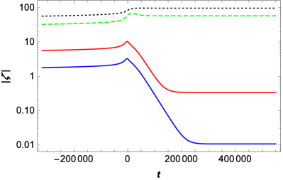
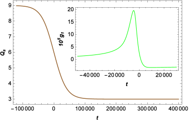
We plot the evolutions of Qssubscript𝑄𝑠Q_{s}, g1subscript𝑔1g_{1}, |ζ|𝜁|\zeta| with respect to t𝑡t, and also Pζ(k)subscript𝑃𝜁𝑘P_{\zeta}(k) for the background in Fig. 2, with different values of {\cal B} and tsubscript𝑡t_{*} in this Appendix.

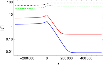
We see how |ζ|𝜁|\zeta| evolves with a𝑎a in different phases. Theoretically, ζ1/asimilar-to𝜁1𝑎\zeta\sim 1/a for the perturbation modes with kzs′′/zsmuch-greater-than𝑘superscriptsubscript𝑧𝑠′′subscript𝑧𝑠k\gg\sqrt{z_{s}^{\prime\prime}/z_{s}}, while ζconst.similar-to𝜁𝑐𝑜𝑛𝑠𝑡\zeta\sim const. for the perturbation modes with kzs′′/zsmuch-less-than𝑘superscriptsubscript𝑧𝑠′′subscript𝑧𝑠k\ll\sqrt{z_{s}^{\prime\prime}/z_{s}}, which is consistent with our Figs. 7(c) and 8(c).
Refer to caption
(a)   Qssubscript𝑄𝑠Q_{s}
Refer to caption
(b)   105×(3H+Q˙s/Qs)superscript1053𝐻subscript˙𝑄𝑠subscript𝑄𝑠10^{5}\times(3H+\dot{Q}_{s}/Q_{s})
Refer to caption
(c)   |ζ|𝜁|\zeta| for k={105,3×105,103,102}𝑘superscript1053superscript105superscript103superscript102k=\{10^{-5},3\times 10^{-5},10^{-3},10^{-2}\} from top to bottom
Refer to caption
(d)   Pζ/Pζinfsubscript𝑃𝜁superscriptsubscript𝑃𝜁𝑖𝑛𝑓P_{\zeta}/P_{\zeta}^{inf}
Figure 7: We set 𝒜Q=3subscript𝒜𝑄3{\cal A}_{Q}=3, =22{\cal B}=2, t=4×10⁴subscript𝑡4superscript104t_{*}=4\times 10^{4} and the background is given by Fig. 2.
Refer to caption
(a)   Qssubscript𝑄𝑠Q_{s}
Refer to caption
(b)   105×(3H+Q˙s/Qs)superscript1053𝐻subscript˙𝑄𝑠subscript𝑄𝑠10^{5}\times(3H+\dot{Q}_{s}/Q_{s})
Refer to caption
(c)   |ζ|𝜁|\zeta| for k={105,3×105,103,102}𝑘superscript1053superscript105superscript103superscript102k=\{10^{-5},3\times 10^{-5},10^{-3},10^{-2}\} from top to bottom
Refer to caption
(d)   Pζ/Pζinfsubscript𝑃𝜁superscriptsubscript𝑃𝜁𝑖𝑛𝑓P_{\zeta}/P_{\zeta}^{inf}
Figure 8: We set 𝒜Q=3subscript𝒜𝑄3{\cal A}_{Q}=3, =1.61.6{\cal B}=1.6, t=3×10⁴subscript𝑡3superscript104t_{*}=3\times 10^{4} and the background is given by Fig. 2.

Appendix C The matrices elements of (2,1)superscript21{\cal{M}}^{(2,1)} and (3,2)superscript32{\cal M}^{(3,2)}

We define l=αaB2k2𝑙𝛼superscriptsubscript𝑎𝐵2superscript𝑘2l=\sqrt{{\alpha}{a}_{B}^{2}-k^{2}}, x1=1/|B|subscript𝑥11subscriptlimit-from𝐵x_{1}=1/|{\cal H}_{B-}|, x2=B+subscript𝑥2subscriptlimit-from𝐵x_{2}={\cal H}_{B+}, y1,2=(ηBηB)subscript𝑦12subscript𝜂limit-from𝐵minus-or-plussubscript𝜂𝐵y_{1,2}=(\eta_{B{\mp}}-\eta_{B}), and have

11(2,1)subscriptsuperscript2111\displaystyle{\cal{M}}^{(2,1)}_{11} =\displaystyle= πx14l[(l+αaB2y1)Hν1(1)(kx1)kHν11(1)(kx1)]ely1,𝜋subscript𝑥14𝑙delimited-[]𝑙𝛼superscriptsubscript𝑎𝐵2subscript𝑦1subscriptsuperscript𝐻1subscript𝜈1𝑘subscript𝑥1𝑘subscriptsuperscript𝐻1subscript𝜈11𝑘subscript𝑥1superscript𝑒𝑙subscript𝑦1\displaystyle{\sqrt{\pi x_{1}}\over 4l}\left[(l+{\alpha}{a}_{B}^{2}y_{1})H^{(1)}_{\nu_{1}}(kx_{1})-kH^{(1)}_{\nu_{1}-1}(kx_{1})\right]e^{-ly_{1}}, (56)
12(2,1)subscriptsuperscript2112\displaystyle{\cal{M}}^{(2,1)}_{12} =\displaystyle= πx14l[(l+αaB2y1)Hν1(2)(kx1)kHν11(2)(kx1)]ely1,𝜋subscript𝑥14𝑙delimited-[]𝑙𝛼superscriptsubscript𝑎𝐵2subscript𝑦1subscriptsuperscript𝐻2subscript𝜈1𝑘subscript𝑥1𝑘subscriptsuperscript𝐻2subscript𝜈11𝑘subscript𝑥1superscript𝑒𝑙subscript𝑦1\displaystyle{\sqrt{\pi x_{1}}\over 4l}\left[(l+{\alpha}{a}_{B}^{2}y_{1})H^{(2)}_{\nu_{1}}(kx_{1})-kH^{(2)}_{\nu_{1}-1}(kx_{1})\right]e^{-ly_{1}}, (57)
21(2,1)subscriptsuperscript2121\displaystyle{\cal{M}}^{(2,1)}_{21} =\displaystyle= πx14l[(lαaB2y1)Hν1(1)(kx1)kHν11(1)(kx1)]ely1,𝜋subscript𝑥14𝑙delimited-[]𝑙𝛼superscriptsubscript𝑎𝐵2subscript𝑦1subscriptsuperscript𝐻1subscript𝜈1𝑘subscript𝑥1𝑘subscriptsuperscript𝐻1subscript𝜈11𝑘subscript𝑥1superscript𝑒𝑙subscript𝑦1\displaystyle{\sqrt{\pi x_{1}}\over 4l}\left[(l-{\alpha}{a}_{B}^{2}y_{1})H^{(1)}_{\nu_{1}}(kx_{1})-kH^{(1)}_{\nu_{1}-1}(kx_{1})\right]e^{ly_{1}}, (58)
22(2,1)subscriptsuperscript2122\displaystyle{\cal{M}}^{(2,1)}_{22} =\displaystyle= πx14l[(lαaB2y1)Hν1(2)(kx1)kHν11(2)(kx1)]ely1,𝜋subscript𝑥14𝑙delimited-[]𝑙𝛼superscriptsubscript𝑎𝐵2subscript𝑦1subscriptsuperscript𝐻2subscript𝜈1𝑘subscript𝑥1𝑘subscriptsuperscript𝐻2subscript𝜈11𝑘subscript𝑥1superscript𝑒𝑙subscript𝑦1\displaystyle{\sqrt{\pi x_{1}}\over 4l}\left[(l-{\alpha}{a}_{B}^{2}y_{1})H^{(2)}_{\nu_{1}}(kx_{1})-kH^{(2)}_{\nu_{1}-1}(kx_{1})\right]e^{ly_{1}}, (59)
11(3,2)subscriptsuperscript3211\displaystyle{\cal{M}}^{(3,2)}_{11} =\displaystyle= iπx22[(lαaB2y2)Hν2(2)(kx2)+kHν21(2)(kx2)]ely2,𝑖𝜋subscript𝑥22delimited-[]𝑙𝛼superscriptsubscript𝑎𝐵2subscript𝑦2subscriptsuperscript𝐻2subscript𝜈2𝑘subscript𝑥2𝑘subscriptsuperscript𝐻2subscript𝜈21𝑘subscript𝑥2superscript𝑒𝑙subscript𝑦2\displaystyle{i\sqrt{\pi x_{2}}\over 2}\left[(l-{\alpha}{a}_{B}^{2}y_{2})H^{(2)}_{\nu_{2}}(kx_{2})+kH^{(2)}_{\nu_{2}-1}(kx_{2})\right]e^{ly_{2}}, (60)
12(3,2)subscriptsuperscript3212\displaystyle{\cal{M}}^{(3,2)}_{12} =\displaystyle= iπx22[(l+αaB2y2)Hν2(2)(kx2)+kHν21(2)(kx2)]ely2,𝑖𝜋subscript𝑥22delimited-[]𝑙𝛼superscriptsubscript𝑎𝐵2subscript𝑦2subscriptsuperscript𝐻2subscript𝜈2𝑘subscript𝑥2𝑘subscriptsuperscript𝐻2subscript𝜈21𝑘subscript𝑥2superscript𝑒𝑙subscript𝑦2\displaystyle{i\sqrt{\pi x_{2}}\over 2}\left[-(l+{\alpha}{a}_{B}^{2}y_{2})H^{(2)}_{\nu_{2}}(kx_{2})+kH^{(2)}_{\nu_{2}-1}(kx_{2})\right]e^{-ly_{2}}, (61)
21(3,2)subscriptsuperscript3221\displaystyle-{\cal{M}}^{(3,2)}_{21} =\displaystyle= iπx22[(lαaB2y2)Hν2(1)(kx2)+kHν21(1)(kx2)]ely2,𝑖𝜋subscript𝑥22delimited-[]𝑙𝛼superscriptsubscript𝑎𝐵2subscript𝑦2subscriptsuperscript𝐻1subscript𝜈2𝑘subscript𝑥2𝑘subscriptsuperscript𝐻1subscript𝜈21𝑘subscript𝑥2superscript𝑒𝑙subscript𝑦2\displaystyle{i\sqrt{\pi x_{2}}\over 2}\left[(l-{\alpha}{a}_{B}^{2}y_{2})H^{(1)}_{\nu_{2}}(kx_{2})+kH^{(1)}_{\nu_{2}-1}(kx_{2})\right]e^{ly_{2}}, (62)
22(3,2)subscriptsuperscript3222\displaystyle-{\cal{M}}^{(3,2)}_{22} =\displaystyle= iπx22[(l+αaB2y2)Hν2(1)(kx2)+kHν21(1)(kx2)]ely2.𝑖𝜋subscript𝑥22delimited-[]𝑙𝛼superscriptsubscript𝑎𝐵2subscript𝑦2subscriptsuperscript𝐻1subscript𝜈2𝑘subscript𝑥2𝑘subscriptsuperscript𝐻1subscript𝜈21𝑘subscript𝑥2superscript𝑒𝑙subscript𝑦2\displaystyle{i\sqrt{\pi x_{2}}\over 2}\left[-(l+{\alpha}{a}_{B}^{2}y_{2})H^{(1)}_{\nu_{2}}(kx_{2})+kH^{(1)}_{\nu_{2}-1}(kx_{2})\right]e^{-ly_{2}}. (63)

References

  • [1] A. H. Guth, Phys. Rev. D 23, 347 (1981).
  • [2] A. D. Linde, Phys. Lett.  108B, 389 (1982).
  • [3] A. Albrecht and P. J. Steinhardt, Phys. Rev. Lett.  48, 1220 (1982).
  • [4] A. A. Starobinsky, Phys. Lett.  91B, 99 (1980).
  • [5] P. A. R. Ade et al. [Planck Collaboration], Astron. Astrophys.  594, A13 (2016) [arXiv:1502.01589 [astro-ph.CO]].
  • [6] P. A. R. Ade et al. [Planck Collaboration], Astron. Astrophys.  594, A20 (2016) [arXiv:1502.02114 [astro-ph.CO]].
  • [7] A. Borde and A. Vilenkin, Phys. Rev. Lett.  72, 3305 (1994) [gr-qc/9312022].
  • [8] A. Borde, A. H. Guth and A. Vilenkin, Phys. Rev. Lett.  90, 151301 (2003) [gr-qc/0110012].
  • [9] J. Khoury, B. A. Ovrut, P. J. Steinhardt and N. Turok, Phys. Rev. D 64, 123522 (2001) [hep-th/0103239].
  • [10] Y. F. Cai, T. Qiu, Y. S. Piao, M. Li and X. Zhang, JHEP 0710, 071 (2007) [arXiv:0704.1090 [gr-qc]].
  • [11] Y. S. Piao and E. Zhou, Phys. Rev. D 68, 083515 (2003) [hep-th/0308080]; Z. G. Liu, J. Zhang and Y. S. Piao, Phys. Rev. D 84, 063508 (2011) [arXiv:1105.5713].
  • [12] P. Creminelli, A. Nicolis and E. Trincherini, JCAP 1011, 021 (2010) [arXiv:1007.0027 [hep-th]].
  • [13] Y. S. Piao, B. Feng and X. m. Zhang, Phys. Rev. D 69, 103520 (2004) [hep-th/0310206]; Y. S. Piao, Phys. Rev. D 71, 087301 (2005) [astro-ph/0502343]; Y. S. Piao, S. Tsujikawa and X. m. Zhang, Class. Quant. Grav.  21, 4455 (2004) [hep-th/0312139].
  • [14] P. A. R. Ade et al. [Planck Collaboration], Astron. Astrophys.  571, A1 (2014) [arXiv:1303.5062 [astro-ph.CO]].
  • [15] P. A. R. Ade et al. [Planck Collaboration], Astron. Astrophys.  594, A16 (2016) [arXiv:1506.07135 [astro-ph.CO]].
  • [16] Y. Cai, Y. T. Wang and Y. S. Piao, Phys. Rev. D 92, 2, 023518 (2015) [arXiv:1501.01730 [astro-ph.CO]].
  • [17] Z. G. Liu, Z. K. Guo and Y. S. Piao, Phys. Rev. D 88, 063539 (2013) [arXiv:1304.6527 [astro-ph.CO]].
  • [18] T. Biswas and A. Mazumdar, Class. Quant. Grav.  31, 025019 (2014) [arXiv:1304.3648 [hep-th]].
  • [19] Z. G. Liu, Z. K. Guo and Y. S. Piao, Eur. Phys. J. C 74, no. 8, 3006 (2014) [arXiv:1311.1599 [astro-ph.CO]].
  • [20] F. T. Falciano, M. Lilley and P. Peter, Phys. Rev. D 77, 083513 (2008) [arXiv:0802.1196 [gr-qc]]; M. Lilley, L. Lorenz and S. Clesse, JCAP 1106, 004 (2011) [arXiv:1104.3494 [gr-qc]].
  • [21] J. Mielczarek, JCAP 0811, 011 (2008) [arXiv:0807.0712 [gr-qc]].
  • [22] J. Q. Xia, Y. F. Cai, H. Li and X. Zhang, Phys. Rev. Lett.  112, 251301 (2014) [arXiv:1403.7623 [astro-ph.CO]].
  • [23] Z. G. Liu, H. Li and Y. S. Piao, Phys. Rev. D 90, no. 8, 083521 (2014) [arXiv:1405.1188 [astro-ph.CO]].
  • [24] T. Qiu and Y. T. Wang, JHEP 1504, 130 (2015) [arXiv:1501.03568 [astro-ph.CO]].
  • [25] Y. Wan, T. Qiu, F. P. Huang, Y. F. Cai, H. Li and X. Zhang, JCAP 1512, no. 12, 019 (2015) [arXiv:1509.08772 [gr-qc]].
  • [26] H. G. Li, Y. Cai and Y. S. Piao, Eur. Phys. J. C 76, no. 12, 699 (2016) [arXiv:1605.09586 [gr-qc]].
  • [27] S. Ni, H. Li, T. Qiu, W. Zheng and X. Zhang, arXiv:1707.05570 [astro-ph.CO].
  • [28] Y. Cai, Y. Wan, H. G. Li, T. Qiu and Y. S. Piao, JHEP 1701, 090 (2017) [arXiv:1610.03400 [gr-qc]].
  • [29] P. Creminelli, D. Pirtskhalava, L. Santoni and E. Trincherini, JCAP 1611, no. 11, 047 (2016) [arXiv:1610.04207 [hep-th]].
  • [30] Y. Cai, H. G. Li, T. Qiu and Y. S. Piao, Eur. Phys. J. C 77, no. 6, 369 (2017) [arXiv:1701.04330 [gr-qc]].
  • [31] Y. Cai and Y. S. Piao, JHEP 1709, 027 (2017) [arXiv:1705.03401 [gr-qc]].
  • [32] R. Kolevatov, S. Mironov, N. Sukhov and V. Volkova, JCAP 1708, no. 08, 038 (2017) [arXiv:1705.06626 [hep-th]].
  • [33] Y. Cai and Y. S. Piao, arXiv:1707.01017 [gr-qc].
  • [34] A. Ijjas and P. J. Steinhardt, Phys. Lett. B 764, 289 (2017) [arXiv:1609.01253 [gr-qc]].
  • [35] M. Libanov, S. Mironov and V. Rubakov, JCAP 1608, no. 08, 037 (2016) [arXiv:1605.05992 [hep-th]].
  • [36] T. Kobayashi, Phys. Rev. D 94, no. 4, 043511 (2016) [arXiv:1606.05831 [hep-th]].
  • [37] R. Kolevatov and S. Mironov, Phys. Rev. D 94, no. 12, 123516 (2016) [arXiv:1607.04099 [hep-th]].
  • [38] S. Akama and T. Kobayashi, Phys. Rev. D 95, no. 6, 064011 (2017) [arXiv:1701.02926 [hep-th]].
  • [39] G. W. Horndeski, Int. J. Theor. Phys.  10, 363 (1974).
  • [40] C. Deffayet, X. Gao, D. A. Steer and G. Zahariade, Phys. Rev. D 84, 064039 (2011) [arXiv:1103.3260 [hep-th]].
  • [41] T. Kobayashi, M. Yamaguchi and J. Yokoyama, Prog. Theor. Phys.  126, 511 (2011) [arXiv:1105.5723 [hep-th]].
  • [42] A. Ijjas and P. J. Steinhardt, Phys. Rev. Lett.  117, no. 12, 121304 (2016) [arXiv:1606.08880 [gr-qc]].
  • [43] D. A. Easson, I. Sawicki and A. Vikman, JCAP 1111, 021 (2011) [arXiv:1109.1047 [hep-th]].
  • [44] D. Langlois and K. Noui, JCAP 1602, no. 02, 034 (2016) [arXiv:1510.06930 [gr-qc]].
  • [45] D. Langlois and K. Noui, JCAP 1607, no. 07, 016 (2016) [arXiv:1512.06820 [gr-qc]].
  • [46] E. I. Buchbinder, J. Khoury and B. A. Ovrut, Phys. Rev. D 76, 123503 (2007) [hep-th/0702154].
  • [47] L. Battarra, M. Koehn, J. L. Lehners and B. A. Ovrut, JCAP 1407, 007 (2014) [arXiv:1404.5067 [hep-th]].
  • [48] M. Koehn, J. L. Lehners and B. Ovrut, Phys. Rev. D 93, 10, 103501 (2016) [arXiv:1512.03807 [hep-th]].
  • [49] Y. F. Cai et.al, JCAP 0803, 013 (2008) [arXiv:0711.2187 [hep-th]].
  • [50] C. R. Contaldi, M. Peloso, L. Kofman and A. D. Linde, JCAP 0307, 002 (2003) [astro-ph/0303636].
  • [51] E. Dudas, N. Kitazawa, S. P. Patil and A. Sagnotti, JCAP 1205, 012 (2012) [arXiv:1202.6630 [hep-th]].
  • [52] S. Das, G. Goswami, J. Prasad and R. Rangarajan, JCAP 1506, no. 06, 001 (2015) [arXiv:1412.7093 [astro-ph.CO]].
  • [53] Y. F. Cai, E. G. M. Ferreira, B. Hu and J. Quintin, Phys. Rev. D 92, no. 12, 121303 (2015) [arXiv:1507.05619 [astro-ph.CO]].
  • [54] K. Wang, L. Santos, J. Q. Xia and W. Zhao, JCAP 1701, no. 01, 053 (2017) [arXiv:1608.04189 [astro-ph.CO]].
  • [55] E. A. Kontou, J. J. Blanco-Pillado, M. P. Hertzberg and A. Masoumi, JCAP 1704, no. 04, 034 (2017) [arXiv:1701.01706 [hep-th]].
  • [56] Y. T. Wang and Y. S. Piao, Phys. Lett. B 741, 55 (2015) [arXiv:1409.7153 [gr-qc]].
  • [57] D. Yoshida, J. Quintin, M. Yamaguchi and R. H. Brandenberger, Phys. Rev. D 96, no. 4, 043502 (2017) [arXiv:1704.04184 [hep-th]].
  • [58] Y. Misonoh, M. Fukushima and S. Miyashita, Phys. Rev. D 95, 4, 044044 (2017) [arXiv:1612.09077 [gr-qc]].
  • [59] M. Giovannini, Phys. Rev. D 95, 8, 083506 (2017) [arXiv:1612.00346 [hep-th]].
  • [60] S. Banerjee and E. N. Saridakis, Phys. Rev. D 95, 6, 063523 (2017) [arXiv:1604.06932 [gr-qc]].
  • [61] T. Biswas, E. Gerwick, T. Koivisto and A. Mazumdar, Phys. Rev. Lett.  108, 031101 (2012) [arXiv:1110.5249 [gr-qc]]; T. Biswas, A. S. Koshelev, A. Mazumdar and S. Y. Vernov, JCAP 1208, 024 (2012) [arXiv:1206.6374 [astro-ph.CO]].
  • [62] M. Vasilic, Phys. Rev. D 95, 12, 123506 (2017) [arXiv:1704.02589 [gr-qc]].
  • [63] Y. B. Li, J. Quintin, D. G. Wang and Y. F. Cai, JCAP 1703, 03, 031 (2017) [arXiv:1612.02036 [hep-th]].
  • [64] S. D. Odintsov and V. K. Oikonomou, Phys. Rev. D 92 (2015) 2, 024016 [arXiv:1504.06866 [gr-qc]]; S. D. Odintsov and V. K. Oikonomou, Phys. Rev. D 91 (2015) 6, 064036 [arXiv:1502.06125 [gr-qc]]; S. D. Odintsov and V. K. Oikonomou, Phys. Rev. D 90 (2014) 12, 124083 [arXiv:1410.8183 [gr-qc]].
  • [65] S. H. Hendi, M. Momennia, B. Eslam Panah and M. Faizal, Astrophys. J.  827, 2, 153 (2016) [arXiv:1703.00480 [gr-qc]]; S. H. Hendi, M. Momennia, B. Eslam Panah and S. Panahiyan, Universe 16, 26 (2017) [arXiv:1705.01099 [gr-qc]].
  • [66] S. Chinaglia, A. Colleaux and S. Zerbini, arXiv:1708.08667 [gr-qc].
  • [67] M. Giovannini, arXiv:1708.08713 [hep-th].
  • [68] S. Farnsworth, J. L. Lehners and T. Qiu, arXiv:1709.03171 [gr-qc].
  • [69] S. Nojiri, S. D. Odintsov and V. K. Oikonomou, Phys. Rept.  692, 1 (2017) [arXiv:1705.11098 [gr-qc]].
  • [70] D. Battefeld and P. Peter, Phys. Rept.  571, 1 (2015) [arXiv:1406.2790 [astro-ph.CO]].