Abstract

We investigate the short distance fate of distinct classes of not asymptotically free supersymmetric gauge theories. Examples include super QCD with two adjoint fields and generalised superpotentials, gauge theories without superpotentials and with two types of matter representation and semi-simple gauge theories such as quivers. We show that for the aforementioned theories asymptotic safety is nonperturbatively compatible with all known constraints.

1 Introduction

The discovery of asymptotic freedom [1, 2] has played an important role in particle physics. According to Wilson [3, 4] these theories are fundamental since they are valid at arbitrary short and long distance scales. Another class of fundamental theories a lá Wilson are the ones featuring an ultraviolet interacting fixed point, and known as asymptotically safe theories. The first proof of existence of asymptotically safe gauge-Yukawa theories in four dimensions appeared in [5]. These type of theories constitute now an important alternative to asymptotic freedom. One can now imagine new extensions of the Standard Model [6, 7, 8, 9, 10] and novel ways to achieve radiative symmetry breaking [6, 7].

In the original construction [5] elementary scalars and their induced Yukawa interactions play a crucial role in helping make the overall gauge-Yukawa theory safe. Quite surprisingly supersymmetric cousins of the original model, such as super QCD (SQCD) with(out) a meson and Yukawa-like superpotentials, do not support asymptotic safety [11]. An alleged UV fixed point, when asymptotic freedom is lost, would typically violate the $a$-theorem [12, 13, 14] inequality [11]. It is possible to go around this constraint, as we shall see in much detail below, by considering theories with multiple fields in distinct matter representations with(out) superpotentials.

The first such example was SQCD with two adjoints, featuring a large enough number of quark superfields [15] and a superpotential. This mechanism has been recently generalized in [16] for phenomenologically motivated SO(10) gauge theories with $3\times 16+10+210+126+\overline{126}$ [17, 18, 19] matter representations. The latter is dictated by the requirement that the $R$-parity [20, 21, 22] is present at all scales [23, 24, 25]. These theories have all $R$-charges uniquely determined because of the presence of the superpotential and the vanishing of the all-order NSVZ beta function [26]. One can consider vanishing superpotentials but then one has to resort to $a$-maximization [27] to determine the $R$-charges. Explicit examples of this type appeared first in [16].

Here we greatly enlarge these families of UV safe supersymmetric examples, and in the process we gain further insight on how to construct nonperturbatively safe supersymmetric QFTs. We also investigate quiver theories in which an interacting UV fixed point flows towards an interacting IR one.

The paper is constructed as follows: In section 2 we investigate SQCD with two adjoint fields and different superpotentials. Section 3 contains a study of SO(10) and SU(5) gauge theories with different types of vector and chiral like matter without superpotential. Quiver theories are studied in Section 4, and we offer our conclusions in section 5.

2 Safe SQCD with two adjoints and superpotential

In [15] Martin and Wells proposed a theory for which the nonperturbative existence of an interacting UV fixed point is not excluded by any known constraints. The model features the following superpotential:

$$W=\mbox{Tr}\,[\tilde{Q}XQ]+\mbox{Tr}\,[X^{3}]\ ,$$ (2.1)

and its field content is summarised in Table [1]. We arrange the number of colours and flavours such that asymptotic freedom is lost and define the quantity $x=N_{c}/N_{f}$. The vanishing of the $\beta$-function for the gauge and holomorphic coupling provides enough constraints to uniquely determine all the $R$-charges of the theory at the would be UV fixed point. Moreover, the anomalous dimensions of the gauge singlet operators do not violate the unitarity bound. The $\Delta a$ between the non trivial fixed point and the IR gaussian turns out to be:

$$\Delta a=a_{FP}-a_{FREE}=\frac{1}{9x}(1-4x)(x-1)^{2}.$$ (2.2)

The non trivial UV fixed point can occur when $x<1/4$.

$$\begin{array}[]{|c|c|c c c c|}\hline\cr{\rm Fields}&\left[SU(N_{c})\right]&SU_{L}(N_{f})&SU_{R}(N_{f})&U_{V}(1)&U(1)_{R}\\ \hline\cr\hline\cr W_{\alpha}&{\rm Adj}&1&1&0&1\\ Q&\raisebox{-0.5pt}{\hbox{\rule{0.4pt}{6.5pt}\hskip-0.4pt\rule{6.5pt}{0.4pt}\hskip-6.5pt\rule[6.5pt]{6.5pt}{0.4pt}}\rule[6.5pt]{0.4pt}{0.4pt}\hskip-0.4pt\rule{0.4pt}{6.5pt}}&\overline{\raisebox{-0.5pt}{\hbox{\rule{0.4pt}{6.5pt}\hskip-0.4pt\rule{6.5pt}{0.4pt}\hskip-6.5pt\rule[6.5pt]{6.5pt}{0.4pt}}\rule[6.5pt]{0.4pt}{0.4pt}\hskip-0.4pt\rule{0.4pt}{6.5pt}}}&1&1&2/3\\ \widetilde{Q}&\overline{\raisebox{-0.5pt}{\hbox{\rule{0.4pt}{6.5pt}\hskip-0.4pt\rule{6.5pt}{0.4pt}\hskip-6.5pt\rule[6.5pt]{6.5pt}{0.4pt}}\rule[6.5pt]{0.4pt}{0.4pt}\hskip-0.4pt\rule{0.4pt}{6.5pt}}}&1&{\raisebox{-0.5pt}{\hbox{\rule{0.4pt}{6.5pt}\hskip-0.4pt\rule{6.5pt}{0.4pt}\hskip-6.5pt\rule[6.5pt]{6.5pt}{0.4pt}}\rule[6.5pt]{0.4pt}{0.4pt}\hskip-0.4pt\rule{0.4pt}{6.5pt}}}&-1&2/3\\ X&{\rm Adj}&1&1&0&2/3\\ Y&{\rm Adj}&1&1&0&\frac{1}{3}\left(1+\frac{N_{f}}{N_{c}}\right)\\ \hline\cr\end{array}$$

Table 1: The ${\cal N}=1$ superfield content with the addition of two gauge adjoint chiral superfield $X,Y$ in the model by Martin and Wells.

It can be shown that this example is part of a larger class of theories defined by the superpotential:

$$W\sim\mbox{Tr}\,[(\tilde{Q}Q)^{n}X^{k_{1}}Y^{k_{2}}]+\mbox{Tr}\,[(\tilde{Q}Q)^{m}X^{l_{1}}Y^{l_{2}}]\ .$$ (2.3)

For some specific choices of $n,k_{1},k_{2},m,l_{1},l_{2}$. The symbol $\sim$ means that we identify all the superpotentials obtained rearranging the fields in different ways that yield the same $R$-charge constraints. The latter together with the vanishing of the NSVZ beta function gives:

$$\begin{split}2nR_{Q}+k_{1}R_{X}+k_{2}R_{Y}=2\ .\\ 2mR_{Q}+l_{1}R_{X}+l_{2}R_{Y}=2\ ,\\ x(R_{X}+R_{Y}-1)+(R_{Q}-1)=\ 0\ .\end{split}$$ (2.4)

To avoid the emergence of free gauge invariants operators we impose:

$$n=0\wedge 2\leq k_{1}+k_{2}\leq 6\quad\vee\quad k_{1}=k_{2}=0\wedge 1\leq n\leq 3.$$ (2.5)

We can find a total of 104 potentials providing UV fixed point satisfying all constraints. Every fixed point satisfies the constraints only in a finite $x$-interval. For example, for $x=0.46$ which is the highest possible value of $x$ allowing an UV interacting fixed point connected to the IR free one, we have seven relevant operators. These potentials read:

$$\begin{split}&W_{1}\sim\mbox{Tr}\,[X^{6}]+\mbox{Tr}\,[\tilde{Q}QX^{4}]\ ,\\ &W_{2}\sim\mbox{Tr}\,[X^{6}]+\mbox{Tr}\,[(\tilde{Q}Q)^{2}X^{2}]\ ,\\ &W_{3}\sim\mbox{Tr}\,[X^{6}]+\mbox{Tr}\,[(\tilde{Q}Q)^{3}]\ ,\\ &W_{4}\sim\mbox{Tr}\,[\tilde{Q}QX^{4}]+\mbox{Tr}\,[(\tilde{Q}Q)^{2}X^{2}]\ ,\\ &W_{5}\sim\mbox{Tr}\,[\tilde{Q}QX^{4}]+\mbox{Tr}\,[(\tilde{Q}Q)^{3}]\ ,\\ &W_{6}\sim\mbox{Tr}\,[(\tilde{Q}Q)^{2}X^{2}]+\mbox{Tr}\,[(\tilde{Q}Q)^{3}]\ ,\\ &W_{7}\sim\mbox{Tr}\,[X^{5}]+\mbox{Tr}\,[(\tilde{Q}Q)^{3}]\ .\\ \end{split}$$ (2.6)

Notice that, at the fixed point, the $R$-charges are the same for the first six potentials implying that the UV value of the $a$-function is the same. Furthermore the $a$-theorem variation in between any of these UV fixed point and the trivial IR one is positive for small $x$.

3 Safety without superpotentials: the SO(10) and SU(5) templates

We had already noticed in [16] that all the known bounds for the possible existence of nonperturbative fixed points

$$\Delta a > 0$$ (3.1)

$$c > 0$$ (3.2)

$$1/6 \leq (a/c)\leq 1/2\ ,$$ (3.3)

are abided with no gauge invariant operators (GIO) with $R<2/3$ by, for example, for an SO(10) theory featuring a very large number of generations respectively in the 10 and 126 representation and with vanishing superpotentials. It is therefore timely to generalise these results.

In the following, the choice of gauge groups SO(10) or SU(5) and their representations is partially inspired by the fundamental role they play in grand unified extensions of the the Standard Model [28, 29, 30]. Supersymmetry is a natural playground for the unification scenario since it almost automatically predicts the correct low energy spectrum that allows for one step-unification of the 3 gauge couplings [31, 32, 33, 34]. As discussed in [16], however, asymptotic freedom is never respected in supersymmetric GUTs such as the ones that predict exact R-parity conservation [20, 21, 22] at low energy [23, 24, 25]. The reason being that one needs large matter representations [18, 17, 35, 19] under SO(10), making our current investigation potentially interesting for this line of research.

3.1 The SO(10) template

We start by considering susy SO(10) theories with $n_{1}$ generations in the representation $r_{1}$ and $n_{2}$ in the representation $r_{2}$ with vanishing superpotential.

We scan for $r_{1}$ and $r_{2}>r_{1}$ over the representations

$$10,16,45,54,120,126,144,210\ .$$ (3.4)

The constraint of no GIO with $R<2/3$ is satisfied by imposing $R>1/3$ for real representations and $R>1/6$ for complex representations and we discover that the only solutions satisfying (3.1)-(3.3) above occur for

$$(r_{1},r_{2})=(10,126),\;(16,126)\ .$$ (3.5)

The number of generations involved is large. The reason being that to abide all the constraints one needs at least $n_{10}\geq 554$, while in the second case $n_{16}\geq 418$. In fact, we now argue that there is an infinite number of such solutions for integer number of generations in the 126 representation. To prove this we note that for $n_{10}\geq 8490$ in the first case and for $n_{16}\geq 6191$ in the second case there is at least one integer value of $n_{2}$ for which all constraints (3.1)-(3.3) are satisfied. Since there is no upper bound on $n_{10}$ or $n_{16}$, there is no upper bound on the number of solutions. We now turn our attention to the possibility of having a smaller number of matter fields, but clearly still above the critical number needed to abide the constraints. We find that the most minimal among these solutions contains $n_{1}=478$ generations of 16 and $n_{2}=19$ generations of 126. For this example we analyze the flow via the Lagrange multiplier technique [36] which for two type of chiral matter reduces to

$$a=2G+n_{1}r_{1}a_{1}(R_{1})+n_{2}r_{2}a_{1}(R_{2})+\lambda_{G}\left(T_{G}+n_{1}T_{1}(R_{1}-1)+n_{2}T_{2}(R_{2}-1)\right)$$ (3.6)

Extremization over $R_{i}$, $i=1,2$, gives

$$R_{i}(\lambda_{G})=1-\frac{\epsilon_{i}}{3}\sqrt{1-\frac{\lambda_{G}T_{i}}{r_{i}}}\;\;\;,\;\;\;\epsilon_{i}^{2}=1$$ (3.7)

In the IR ($\lambda_{G}=0$) the theory is free, so we are in the $\epsilon_{1,2}=+1$ branch. The flow goes from the IR towards positive $\lambda_{G}$ (that it must be positive here we know from perturbative calculations which are applicable for small enough $\lambda_{G}\sim g^{2}$) until it reaches

$$\lambda_{G}^{max}\equiv Min(r_{i}/T_{i})$$ (3.8)

which is, in the two cases (3.5), always given by $126$:

$$\lambda_{G}^{max}=\frac{126}{35}=\frac{18}{5}=3.6$$ (3.9)

At this point $\epsilon_{126}$ changes sign. $\lambda_{G}$ can now only decrease (increasing above $\lambda_{G}^{max}$ would lead to complex value for $R_{126}$), but now in the branch $\epsilon_{16}=+1$, $\epsilon_{126}=-1$. We pass through $\lambda_{G}=0$ (which is no more a free theory, because of the different branch) towards negative values of $\lambda_{G}$, all the way to the fixed point value of

$$\lambda_{G}^{*}=-41.63$$ (3.10)

for which (having $a(0)=20894/9$):

$$(R_{16},R_{126})(\lambda_{G}^{*}) = (0.1697,2.1816)$$ (3.11)

$$a(\lambda_{G}^{*}) = 2326.5$$ (3.12)

$$\Delta a(\lambda_{G}^{*}) = 4.955$$ (3.13)

$$c(\lambda_{G}^{*}) = 13932.1$$ (3.14)

$$(a/c)(\lambda_{G}^{*})-1/6 = 3.2\times 10^{-4}$$ (3.15)

Notice that $4R_{16}>2/3$ but in order to avoid a free field with $R=2R_{16}<2/3$ we need to have only $16$ or only $\overline{16}$ but not both. This is not necessary for the $126$ for which the $R_{126}$ is safely large. The flows of the different quantities are shown in Fig. [1].

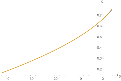
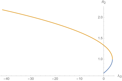
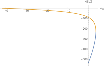
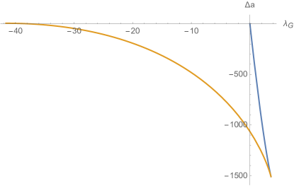
Figure 1: Flows of $R_{1}$ (upper left), $R_{2}$ (upper right), the $NSVZ$ function (lower left) and $\Delta a$ (lower right) as functions of the Lagrange multiplier $\lambda_{G}$. The blue (orange) curves show the direction of the flow towards increasing (decreasing) $\lambda_{G}$. The starting points of the blue curves at $\lambda_{G}=0$ are at the free IR theory.

We have therefore found an entire family of solutions that can be asymptotically safe. Furthermore, the fact that there is a critical number of matter field value above which the asymptotically safe theory emerges within infrared gauge-matter free theories can be viewed as the supersymmetric analogue of the large $N_{f}$ solutions of non-supersymmetric safe non-abelian gauge-fermion theories recently discussed in [37].

3.2 The SU(5) template

One can repeat the above analysis for SU(5). Considering only fields up to representation 75, i.e. over

$$5,10,15,24,35,40,45,50,70,70^{\prime},75$$ (3.16)

(and their conjugates) only the following pairs can lead to consistent UV fixed point and free IR limits (to be on the safe side we impose here $R_{i}\geq 1/3$ for all, real or complex representations; also, we assume that the $R$ charges of a field in representation $r$ is the same as the $R$ charge of an eventual field in the conjugate representation $\bar{r}$):

$$(r_{1},r_{2})=(5,35),(5,40),(5,70),(5,70^{\prime}),(5,75),(10,70^{\prime}),(24,70^{\prime})$$ (3.17)

Differently from SO(10), these SU(5) examples are not automatically anomaly free. To be so they must satisfy

$$(n_{1}-n_{\bar{1}})A_{1}+(n_{2}-n_{\bar{2}})A_{2}=0$$ (3.18)

where $n_{a}(n_{\bar{a}})$ is the number of generations of representation $r_{a}(\bar{r}_{a})$, $a=1,2$, and the anomaly coefficients $A_{i}$ are given for representations $r_{i}$ on Table [2].

$r_{i}$	5	10	15	24	35	40	45	50	70	$70^{\prime}$	75
$A_{i}$	1	1	9	0	-44	-16	-6	-15	29	-156	0

Table 2: The anomaly coefficients for representations smaller or equal to 75.

There are infinite number of solutions, let s present those with the minimal number of generations, taking into account only solutions with

$$n_{1}+n_{\bar{1}}\leq 1000\;\;\;,\;\;\;n_{2}+n_{\bar{2}}\leq 5$$ (3.19)

We summarise them in Table [3]. Some of them are chiral, some are vectorlike. Other solutions with the same number of fields are also possible. For example the second row can also have a vectorlike possibility with $(61+119)/2=90$ copies of $5+\bar{5}$ and one generation of $70+\overline{70}$. The opposite is not necessarily true, see the model in the last row where a chiral possibility is not present. Notice that in order to have the precision in $\Delta a$ as specified in Table [3] we had to specify $R_{1,2}$ with higher precision, since cancellations are at work.

$r_{1}$	$n_{1}$	$n_{\bar{1}}$	$R_{1}=R_{\bar{1}}$	$r_{2}$	$n_{2}$	$n_{\bar{2}}$	$R_{2}=R_{\bar{2}}$	$\Delta a$	$c_{UV}$	$(a/c)_{UV}$
5	15	147	0.43695	35	0	3	1.96684	2.15	1422.	0.178
5	61	119	0.36651	70	2	0	2.06152	6.38	1652.	0.173
5	9	165	0.54917	70’	0	1	1.81481	0.75	1395.	0.185
5	90	90	0.35869	75	2	-	2.05436	0.99	1637.	0.172
10	51	51	0.43853	70’	1	1	1.96316	13.70	1786.	0.179

Table 3: The candidates for UV fixed points with the minimal number of generations.

These new families of solutions show that supersymmetric gauge theories with(out) chiral matter and without superpotential can be asymptotically safe above a critical number of matter fields. Our results complement the investigation for non supersymmetric chiral gauge theories performed first in [38]. Our analysis, can be straightforwardly extended to other gauge groups with similar matter content. One can also relax the constraints on the absence of GIO operators but this will be explored elsewhere.

4 Semi-simple gauge groups

Here we will analyse examples of semi-simple gauge groups starting with the quivers of [27, 39].

4.1 The SU(N)⁴ quiver

The field content of the theory along with the gauge and SU(2) flavor symmetries and charges are shown in Table [4]. In the $N\to\infty$ limit one recovers the U(N)⁴ case. We consider a superpotential that respects all the symmetries:

$$W = y_{1}{\cal O}_{1}+y_{2}{\cal O}_{2}+y_{3}{\cal O}_{3}$$ (4.1)

$$= {\rm Tr}\left[y_{1}\epsilon_{ab}X_{21}^{a}X_{14}^{b}X_{42}+y_{2}\epsilon_{ab}X_{21}^{a}X_{13}X_{32}^{b}+y_{3}\epsilon_{ab}X_{21}^{3}X_{14}^{a}X_{43}X_{32}^{b}\right].$$

$$\begin{array}[]{|c|c c c c c|}\hline\cr{\rm Fields}&\left[SU(N)_{1}\right]&\left[SU(N)_{2}\right]&\left[SU(N)_{3}\right]&\left[SU(N)_{4}\right]&SU(2)_{F}\\ \hline\cr\hline\cr X_{21}^{a}&\overline{\raisebox{-0.5pt}{\hbox{\rule{0.4pt}{6.5pt}\hskip-0.4pt\rule{6.5pt}{0.4pt}\hskip-6.5pt\rule[6.5pt]{6.5pt}{0.4pt}}\rule[6.5pt]{0.4pt}{0.4pt}\hskip-0.4pt\rule{0.4pt}{6.5pt}}}&\raisebox{-0.5pt}{\hbox{\rule{0.4pt}{6.5pt}\hskip-0.4pt\rule{6.5pt}{0.4pt}\hskip-6.5pt\rule[6.5pt]{6.5pt}{0.4pt}}\rule[6.5pt]{0.4pt}{0.4pt}\hskip-0.4pt\rule{0.4pt}{6.5pt}}&1&1&\raisebox{-0.5pt}{\hbox{\rule{0.4pt}{6.5pt}\hskip-0.4pt\rule{6.5pt}{0.4pt}\hskip-6.5pt\rule[6.5pt]{6.5pt}{0.4pt}}\rule[6.5pt]{0.4pt}{0.4pt}\hskip-0.4pt\rule{0.4pt}{6.5pt}}\\ X_{21}^{3}&\overline{\raisebox{-0.5pt}{\hbox{\rule{0.4pt}{6.5pt}\hskip-0.4pt\rule{6.5pt}{0.4pt}\hskip-6.5pt\rule[6.5pt]{6.5pt}{0.4pt}}\rule[6.5pt]{0.4pt}{0.4pt}\hskip-0.4pt\rule{0.4pt}{6.5pt}}}&\raisebox{-0.5pt}{\hbox{\rule{0.4pt}{6.5pt}\hskip-0.4pt\rule{6.5pt}{0.4pt}\hskip-6.5pt\rule[6.5pt]{6.5pt}{0.4pt}}\rule[6.5pt]{0.4pt}{0.4pt}\hskip-0.4pt\rule{0.4pt}{6.5pt}}&1&1&1\\ X_{14}^{a}&\raisebox{-0.5pt}{\hbox{\rule{0.4pt}{6.5pt}\hskip-0.4pt\rule{6.5pt}{0.4pt}\hskip-6.5pt\rule[6.5pt]{6.5pt}{0.4pt}}\rule[6.5pt]{0.4pt}{0.4pt}\hskip-0.4pt\rule{0.4pt}{6.5pt}}&1&1&\overline{\raisebox{-0.5pt}{\hbox{\rule{0.4pt}{6.5pt}\hskip-0.4pt\rule{6.5pt}{0.4pt}\hskip-6.5pt\rule[6.5pt]{6.5pt}{0.4pt}}\rule[6.5pt]{0.4pt}{0.4pt}\hskip-0.4pt\rule{0.4pt}{6.5pt}}}&\raisebox{-0.5pt}{\hbox{\rule{0.4pt}{6.5pt}\hskip-0.4pt\rule{6.5pt}{0.4pt}\hskip-6.5pt\rule[6.5pt]{6.5pt}{0.4pt}}\rule[6.5pt]{0.4pt}{0.4pt}\hskip-0.4pt\rule{0.4pt}{6.5pt}}\\ X_{43}&1&1&\overline{\raisebox{-0.5pt}{\hbox{\rule{0.4pt}{6.5pt}\hskip-0.4pt\rule{6.5pt}{0.4pt}\hskip-6.5pt\rule[6.5pt]{6.5pt}{0.4pt}}\rule[6.5pt]{0.4pt}{0.4pt}\hskip-0.4pt\rule{0.4pt}{6.5pt}}}&\raisebox{-0.5pt}{\hbox{\rule{0.4pt}{6.5pt}\hskip-0.4pt\rule{6.5pt}{0.4pt}\hskip-6.5pt\rule[6.5pt]{6.5pt}{0.4pt}}\rule[6.5pt]{0.4pt}{0.4pt}\hskip-0.4pt\rule{0.4pt}{6.5pt}}&1\\ X_{32}^{a}&1&\overline{\raisebox{-0.5pt}{\hbox{\rule{0.4pt}{6.5pt}\hskip-0.4pt\rule{6.5pt}{0.4pt}\hskip-6.5pt\rule[6.5pt]{6.5pt}{0.4pt}}\rule[6.5pt]{0.4pt}{0.4pt}\hskip-0.4pt\rule{0.4pt}{6.5pt}}}&\raisebox{-0.5pt}{\hbox{\rule{0.4pt}{6.5pt}\hskip-0.4pt\rule{6.5pt}{0.4pt}\hskip-6.5pt\rule[6.5pt]{6.5pt}{0.4pt}}\rule[6.5pt]{0.4pt}{0.4pt}\hskip-0.4pt\rule{0.4pt}{6.5pt}}&1&\raisebox{-0.5pt}{\hbox{\rule{0.4pt}{6.5pt}\hskip-0.4pt\rule{6.5pt}{0.4pt}\hskip-6.5pt\rule[6.5pt]{6.5pt}{0.4pt}}\rule[6.5pt]{0.4pt}{0.4pt}\hskip-0.4pt\rule{0.4pt}{6.5pt}}\\ X_{13}&\raisebox{-0.5pt}{\hbox{\rule{0.4pt}{6.5pt}\hskip-0.4pt\rule{6.5pt}{0.4pt}\hskip-6.5pt\rule[6.5pt]{6.5pt}{0.4pt}}\rule[6.5pt]{0.4pt}{0.4pt}\hskip-0.4pt\rule{0.4pt}{6.5pt}}&1&\overline{\raisebox{-0.5pt}{\hbox{\rule{0.4pt}{6.5pt}\hskip-0.4pt\rule{6.5pt}{0.4pt}\hskip-6.5pt\rule[6.5pt]{6.5pt}{0.4pt}}\rule[6.5pt]{0.4pt}{0.4pt}\hskip-0.4pt\rule{0.4pt}{6.5pt}}}&1&1\\ X_{42}&1&\overline{\raisebox{-0.5pt}{\hbox{\rule{0.4pt}{6.5pt}\hskip-0.4pt\rule{6.5pt}{0.4pt}\hskip-6.5pt\rule[6.5pt]{6.5pt}{0.4pt}}\rule[6.5pt]{0.4pt}{0.4pt}\hskip-0.4pt\rule{0.4pt}{6.5pt}}}&1&\raisebox{-0.5pt}{\hbox{\rule{0.4pt}{6.5pt}\hskip-0.4pt\rule{6.5pt}{0.4pt}\hskip-6.5pt\rule[6.5pt]{6.5pt}{0.4pt}}\rule[6.5pt]{0.4pt}{0.4pt}\hskip-0.4pt\rule{0.4pt}{6.5pt}}&1\\ \hline\cr\end{array}$$

Table 4: The quantum numbers of the field content in the quiver example.

We study the following cases:

1. if $y_{3}=0$ there is a free field solution, with all $R_{i}=2/3$ and

   $$\frac{a}{N^{2}} = \frac{92}{9}-\frac{8}{N^{2}}\xrightarrow{N\to\infty}10.2$$ (4.2)

   $$\frac{a}{c} = \frac{23-18/N^{2}}{66-36/N^{2}}\xrightarrow{N\to\infty}0.348$$ (4.3)

2. if $y_{1}=y_{2}=y_{3}=0$ (i.e. $W=0$) we have [27]

   $$\frac{a}{N^{2}} = \frac{2}{3}\left(3+5\sqrt{5}\right)-\frac{8}{N^{2}}\xrightarrow{N\to\infty}9.45$$ (4.4)

   $$\frac{a}{c} = \frac{\frac{2}{3}\left(3+5\sqrt{5}\right)-\frac{8}{N^{2}}}{2\left(3+5\sqrt{5}\right)-\frac{16}{N^{2}}}\xrightarrow{N\to\infty}\frac{1}{3}$$ (4.5)

   The $R$-charges of the operators defined in (4.1) are independent on $N$ and equal to

   $$R({\cal O}_{1})=1.87\;\;\;,\;\;\;R({\cal O}_{2})=1.87\;\;\;,\;\;\;R({\cal O}_{3})=2.25$$ (4.6)

3. finally, if any of the $y_{i}\neq 0$ (i.e. if $W\neq 0$), we get [39]

   $$\frac{a}{N^{2}} = \frac{32}{3}\left(-46+13\sqrt{13}\right)-\frac{8}{N^{2}}\xrightarrow{N\to\infty}9.30$$ (4.7)

   $$\ \frac{a}{c} = \frac{\frac{32}{3}\left(-46+13\sqrt{13}\right)-\frac{8}{N^{2}}}{32\left(-46+13\sqrt{13}\right)-\frac{16}{N^{2}}}\xrightarrow{N\to\infty}\frac{1}{3}$$ (4.8)

   The $R$-charges of the operators defined in (4.1) are

   $$R({\cal O}_{1})=2\;\;\;,\;\;\;R({\cal O}_{2})=2\;\;\;,\;\;\;R({\cal O}_{3})=2$$ (4.9)

In the limit $N\to\infty$, the ratio $a/c$ approaches $1/3$ for the case of point 2 and 3, in agreement with the large $N$ expectation for superconformal quivers [40, 41] .

Requiring

(a) $\Delta a\equiv a_{UV}-a_{IR}>0$,

(b) if $y_{i}\neq 0$ then $R({\cal O}_{i})\geq 2$ in the IR and $R({\cal O}_{i})\leq 2$ in the UV,

we find that the only UV safe flow is for a vanishing superpotential $W=0$ in the UV (case 2) and for an interacting $W\neq 0$ but with $y_{3}=0$ in the IR (case 3); in this scenario we have both an IR and an UV interacting fixed point.

4.2 An SU(N₁)$\otimes$SU(N₂) example

Theories with safe trajectories for semisimple gauge groups were first analysed and discovered in [42]. For these theories it is possible to achieve RG trajectories connecting UV and IR interacting fixed points. A supersymmetric model of this type was considered in [43] which can be also viewed as a variant of the $SU(N)^{4}$ quiver in which one gauges two of the previous non-abelian flavour symmetries. We summarise in Table [5] the field content.

$$\begin{array}[]{|c|c c c c|}\hline\cr{\rm Fields}&\left[SU(N_{1})\right]&\left[SU(N_{2})\right]&SU(N_{f})&SU(N_{q})\\ \hline\cr\hline\cr{\psi}&\raisebox{-0.5pt}{\hbox{\rule{0.4pt}{6.5pt}\hskip-0.4pt\rule{6.5pt}{0.4pt}\hskip-6.5pt\rule[6.5pt]{6.5pt}{0.4pt}}\rule[6.5pt]{0.4pt}{0.4pt}\hskip-0.4pt\rule{0.4pt}{6.5pt}}&1&\overline{\raisebox{-0.5pt}{\hbox{\rule{0.4pt}{6.5pt}\hskip-0.4pt\rule{6.5pt}{0.4pt}\hskip-6.5pt\rule[6.5pt]{6.5pt}{0.4pt}}\rule[6.5pt]{0.4pt}{0.4pt}\hskip-0.4pt\rule{0.4pt}{6.5pt}}}&1\\ \widetilde{\psi}&\overline{\raisebox{-0.5pt}{\hbox{\rule{0.4pt}{6.5pt}\hskip-0.4pt\rule{6.5pt}{0.4pt}\hskip-6.5pt\rule[6.5pt]{6.5pt}{0.4pt}}\rule[6.5pt]{0.4pt}{0.4pt}\hskip-0.4pt\rule{0.4pt}{6.5pt}}}&1&\raisebox{-0.5pt}{\hbox{\rule{0.4pt}{6.5pt}\hskip-0.4pt\rule{6.5pt}{0.4pt}\hskip-6.5pt\rule[6.5pt]{6.5pt}{0.4pt}}\rule[6.5pt]{0.4pt}{0.4pt}\hskip-0.4pt\rule{0.4pt}{6.5pt}}&1\\ \Psi&\raisebox{-0.5pt}{\hbox{\rule{0.4pt}{6.5pt}\hskip-0.4pt\rule{6.5pt}{0.4pt}\hskip-6.5pt\rule[6.5pt]{6.5pt}{0.4pt}}\rule[6.5pt]{0.4pt}{0.4pt}\hskip-0.4pt\rule{0.4pt}{6.5pt}}&\raisebox{-0.5pt}{\hbox{\rule{0.4pt}{6.5pt}\hskip-0.4pt\rule{6.5pt}{0.4pt}\hskip-6.5pt\rule[6.5pt]{6.5pt}{0.4pt}}\rule[6.5pt]{0.4pt}{0.4pt}\hskip-0.4pt\rule{0.4pt}{6.5pt}}&1&1\\ \widetilde{\Psi}&\overline{\raisebox{-0.5pt}{\hbox{\rule{0.4pt}{6.5pt}\hskip-0.4pt\rule{6.5pt}{0.4pt}\hskip-6.5pt\rule[6.5pt]{6.5pt}{0.4pt}}\rule[6.5pt]{0.4pt}{0.4pt}\hskip-0.4pt\rule{0.4pt}{6.5pt}}}&\overline{\raisebox{-0.5pt}{\hbox{\rule{0.4pt}{6.5pt}\hskip-0.4pt\rule{6.5pt}{0.4pt}\hskip-6.5pt\rule[6.5pt]{6.5pt}{0.4pt}}\rule[6.5pt]{0.4pt}{0.4pt}\hskip-0.4pt\rule{0.4pt}{6.5pt}}}&1&1\\ \widetilde{\chi}&1&\overline{\raisebox{-0.5pt}{\hbox{\rule{0.4pt}{6.5pt}\hskip-0.4pt\rule{6.5pt}{0.4pt}\hskip-6.5pt\rule[6.5pt]{6.5pt}{0.4pt}}\rule[6.5pt]{0.4pt}{0.4pt}\hskip-0.4pt\rule{0.4pt}{6.5pt}}}&\raisebox{-0.5pt}{\hbox{\rule{0.4pt}{6.5pt}\hskip-0.4pt\rule{6.5pt}{0.4pt}\hskip-6.5pt\rule[6.5pt]{6.5pt}{0.4pt}}\rule[6.5pt]{0.4pt}{0.4pt}\hskip-0.4pt\rule{0.4pt}{6.5pt}}&1\\ {\chi}&1&\raisebox{-0.5pt}{\hbox{\rule{0.4pt}{6.5pt}\hskip-0.4pt\rule{6.5pt}{0.4pt}\hskip-6.5pt\rule[6.5pt]{6.5pt}{0.4pt}}\rule[6.5pt]{0.4pt}{0.4pt}\hskip-0.4pt\rule{0.4pt}{6.5pt}}&\overline{\raisebox{-0.5pt}{\hbox{\rule{0.4pt}{6.5pt}\hskip-0.4pt\rule{6.5pt}{0.4pt}\hskip-6.5pt\rule[6.5pt]{6.5pt}{0.4pt}}\rule[6.5pt]{0.4pt}{0.4pt}\hskip-0.4pt\rule{0.4pt}{6.5pt}}}&1\\ \widetilde{Q}&1&\overline{\raisebox{-0.5pt}{\hbox{\rule{0.4pt}{6.5pt}\hskip-0.4pt\rule{6.5pt}{0.4pt}\hskip-6.5pt\rule[6.5pt]{6.5pt}{0.4pt}}\rule[6.5pt]{0.4pt}{0.4pt}\hskip-0.4pt\rule{0.4pt}{6.5pt}}}&1&\raisebox{-0.5pt}{\hbox{\rule{0.4pt}{6.5pt}\hskip-0.4pt\rule{6.5pt}{0.4pt}\hskip-6.5pt\rule[6.5pt]{6.5pt}{0.4pt}}\rule[6.5pt]{0.4pt}{0.4pt}\hskip-0.4pt\rule{0.4pt}{6.5pt}}\\ {Q}&1&\raisebox{-0.5pt}{\hbox{\rule{0.4pt}{6.5pt}\hskip-0.4pt\rule{6.5pt}{0.4pt}\hskip-6.5pt\rule[6.5pt]{6.5pt}{0.4pt}}\rule[6.5pt]{0.4pt}{0.4pt}\hskip-0.4pt\rule{0.4pt}{6.5pt}}&1&\overline{\raisebox{-0.5pt}{\hbox{\rule{0.4pt}{6.5pt}\hskip-0.4pt\rule{6.5pt}{0.4pt}\hskip-6.5pt\rule[6.5pt]{6.5pt}{0.4pt}}\rule[6.5pt]{0.4pt}{0.4pt}\hskip-0.4pt\rule{0.4pt}{6.5pt}}}\\ \hline\cr\end{array}$$

Table 5: Field content of the model introduced in [43]

The model features in addition a Yukawa-type superpotential of the form:

$$W=y\left(\mbox{Tr}\,[\psi\widetilde{\Psi}\chi]+\mbox{Tr}\,[\widetilde{\psi}{\Psi}\widetilde{\chi}]\right)\ .$$ (4.10)

We will consider the model in the Veneziano limit keeping the following ratios fixed:

$$x_{1}=\frac{N_{1}}{N_{f}}\ ,\quad x_{2}=\frac{N_{2}}{N_{f}}\ ,\quad x_{q}=\frac{N_{q}}{N_{f}}\ .$$ (4.11)

The $\beta$ function for the gauge and superpotential couplings are:

$$\begin{split}&\beta_{y}=\frac{3}{2}y(R_{\psi}+R_{\Psi}+R_{\chi}-2)\\ &\beta_{1}=-\frac{3g_{1}^{3}}{16\pi^{2}}f(g_{1}^{2})[x_{1}+(R_{\psi}-1)-x_{2}(R_{\Psi}-1)]\\ &\beta_{2}=-\frac{3g_{2}^{3}}{16\pi^{2}}f(g_{2}^{2})[x_{2}-(R_{\chi}-1)+x_{1}(R_{\Psi}-1)+x_{q}(R_{Q}-1)]\\ \end{split}$$ (4.12)

where $f(g^{2})\sim 1+O(g^{2})$ is a scheme dependent function of the couplings. The properly normalized $a$-function reads:

$$\begin{split}&a/N_{f}^{2}=2(x_{1}^{2}+x_{2}^{2})+2x_{1}a_{1}(R_{\psi})+2x_{2}a_{1}(R_{\chi})+2x_{1}x_{2}a_{1}(R_{\Psi})+2x_{q}x_{2}a_{1}(R_{Q}).\end{split}$$ (4.13)

We can now find the nonperturbative fixed points of the theory by setting to zero the beta functions together with a-maximisation. We also allow for partially interacting fixed points, following [42], meaning that some of the beta functions vanish trivially at the origin of their respective couplings. To compare our nonperturbative results with the perturbative ones given in [43] we introduce the further quantities:

$$P_{1}=\frac{x_{2}}{x_{1}}\ ,\quad P_{2}=\frac{x_{2}}{x_{1}}\frac{x_{q}+x_{1}-3x_{2}+1}{x_{2}-3x_{1}+1}\ ,\quad\epsilon=\frac{x_{2}-3x_{1}+1}{x_{1}}\ ,$$ (4.14)

and assume $P_{1}=3/2$ and $P_{2}=-5$ while, differently from [43], our $\epsilon$ can take any positive value in the range $]0,0.16776]$ for which no free GIO can emerge. We find seven distinct potential fixed points including the fully non-interacting one in all couplings that pass all the known nonperturbative tests. Of these fixed points three are the physical ones that go over the perturbative analysis. Ordering in the descending value assumed by the central charge $a$ these are the gaussian fixed point at the origin $G$ of all couplings, the interacting (FP_2y) in all couplings except $\alpha_{1}$ and the fully interacting one (FP_12y). We report in Fig. 2 the nonperturbative $R$ charges for the (semi)interacting fixed points as functions of $\epsilon$.

With these charges we plot in Fig. [3] the value of $a$ and $a/c$ as functions of $\epsilon$.

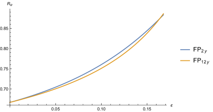
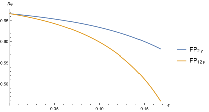
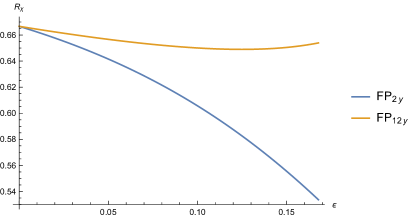
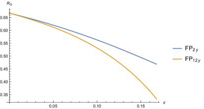
Figure 2: Here we draw the $R$-charges as function of the parameter $\epsilon$ for fixed $P_{1}=3/2$ and $P_{2}=-5$.

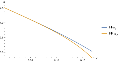
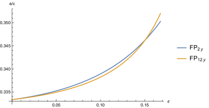
Figure 3: $a$ and $a/c$ as a functions of $\epsilon$ for the (semi)interacting fixed points.

It is clear from the figure that all bounds are respected and that furthermore the highest value of $a$ is for FP_2y suggesting that if a flow exists between this and the fully interacting fixed point, it can be seen as an ultraviolet safe fixed point along this trajectory. This is the susy equivalent of the phenomenon discovered in [42]. In addition we also notice that the fully gaussian fixed point has the highest possible value of $a$ establishing an hierarchy of UV fixed points according to which, de facto, any phenomenological interesting field theory of this type would eventually flow to the fully gaussian one. This is substantially different from the case of [5] in which, at least perturbatively, the only UV fixed point has the maximum $a$. In addition we expect no separatrix directly connecting FP_12y with the gaussian fixed point but a separatrix along the $\alpha_{2}$ coupling direction connecting it to FP_2y because the linearised flow around the gaussian fixed point must necessarely coincide with the perturbative analysis.

5 Conclusions

We studied the short distance behaviour of several distinct classes of not asymptotically free supersymmetric gauge theories. In particular we investigated super QCD with two adjoint fields and generalised superpotentials. Here we showed that nonperturbative asymptotic safety can be achieved without violating the known constraints provided the superpotentials assume specific forms.

We also investigated the emergence of asymptotic safety within supersymmetric field theories featuring only gauge interactions. We discovered that asymptotic safety can be achieved at the cost of introducing a large enough number of matter fields in distinct representations of the gauge groups. In addition we investigated also semi-simple gauge theories with superpotentials such as quiver theories, and demonstrated that asymptotic safety can be achieved as well. Here the mechanism at play requires connecting the UV safe theory to an interacting IR one.

Our results integrate and extend the initial work of Ref. [11] by introducing new mechanisms to achieve supersymmetric safety.

Acknowledgments

BB acknowledges the financial support from the Slovenian Research Agency (research core funding No. P1-0035). The work of ND and FS is partially supported by the Danish National Research Foundation under the grant DNRF:90. BB thanks the CERN theoretical physics division for the hospitality.

References

- [1] D. J. Gross and F. Wilczek, Phys. Rev. D 8, 3633 (1973).
- [2] H. D. Politzer, Phys. Rev. Lett. 30, 1346 (1973).
- [3] K. G. Wilson, Phys. Rev. B 4, 3174 (1971).
- [4] K. G. Wilson, Phys. Rev. B 4, 3184 (1971).
- [5] D. F. Litim and F. Sannino, JHEP 1412, 178 (2014) [arXiv:1406.2337 [hep-th]].
- [6] S. Abel and F. Sannino, Published in Phys. Rev. D. arXiv:1704.00700 [hep-ph].
- [7] S. Abel and F. Sannino, Phys. Rev. D 96, no. 5, 055021 (2017) [arXiv:1707.06638 [hep-ph]].
- [8] G. M. Pelaggi, F. Sannino, A. Strumia and E. Vigiani, arXiv:1701.01453 [hep-ph].
- [9] R. Mann, J. Meffe, F. Sannino, T. Steele, Z. W. Wang and C. Zhang, arXiv:1707.02942 [hep-ph].
- [10] G. M. Pelaggi, A. D. Plascencia, A. Salvio, F. Sannino, J. Smirnov and A. Strumia, arXiv:1708.00437 [hep-ph].
- [11] K. Intriligator and F. Sannino, JHEP 1511, 023 (2015) [arXiv:1508.07411 [hep-th]].
- [12] J. L. Cardy, Phys. Lett. B 215, 749 (1988).
- [13] Z. Komargodski and A. Schwimmer, JHEP 1112, 099 (2011) [arXiv:1107.3987 [hep-th]].
- [14] Z. Komargodski, JHEP 1207, 069 (2012) [arXiv:1112.4538 [hep-th]].
- [15] S. P. Martin and J. D. Wells, Phys. Rev. D 64, 036010 (2001) [hep-ph/0011382].
- [16] B. Bajc and F. Sannino, JHEP 1612, 141 (2016) [arXiv:1610.09681 [hep-th]].
- [17] T. E. Clark, T. K. Kuo and N. Nakagawa, Phys. Lett. 115B, 26 (1982).
- [18] C. S. Aulakh and R. N. Mohapatra, Phys. Rev. D 28, 217 (1983).
- [19] C. S. Aulakh, B. Bajc, A. Melfo, G. Senjanovic and F. Vissani, Phys. Lett. B 588, 196 (2004) [hep-ph/0306242].
- [20] R. N. Mohapatra, Phys. Rev. D 34, 3457 (1986).
- [21] A. Font, L. E. Ibanez and F. Quevedo, Phys. Lett. B 228, 79 (1989).
- [22] S. P. Martin, Phys. Rev. D 46, R2769 (1992) [hep-ph/9207218].
- [23] C. S. Aulakh, K. Benakli and G. Senjanovic, Phys. Rev. Lett. 79, 2188 (1997) [hep-ph/9703434].
- [24] C. S. Aulakh, A. Melfo and G. Senjanovic, Phys. Rev. D 57, 4174 (1998) [hep-ph/9707256].
- [25] C. S. Aulakh, A. Melfo, A. Rasin and G. Senjanovic, Phys. Lett. B 459, 557 (1999) [hep-ph/9902409].
- [26] V. A. Novikov, M. A. Shifman, A. I. Vainshtein and V. I. Zakharov, Nucl. Phys. B 229, 381 (1983).
- [27] K. A. Intriligator and B. Wecht, Nucl. Phys. B 667, 183 (2003) [hep-th/0304128].
- [28] J. C. Pati and A. Salam, Phys. Rev. D 10, 275 (1974) Erratum: [Phys. Rev. D 11, 703 (1975)].
- [29] H. Georgi and S. L. Glashow, Phys. Rev. Lett. 32, 438 (1974).
- [30] H. Georgi, H. R. Quinn and S. Weinberg, Phys. Rev. Lett. 33, 451 (1974).
- [31] S. Dimopoulos, S. Raby and F. Wilczek, Phys. Rev. D 24, 1681 (1981).
- [32] L. E. Ibanez and G. G. Ross, Phys. Lett. 105B, 439 (1981).
- [33] M. B. Einhorn and D. R. T. Jones, Nucl. Phys. B 196, 475 (1982).
- [34] W. J. Marciano and G. Senjanovic, Phys. Rev. D 25, 3092 (1982).
- [35] K. S. Babu and R. N. Mohapatra, Phys. Rev. Lett. 70, 2845 (1993) [hep-ph/9209215].
- [36] D. Kutasov, hep-th/0312098.
- [37] O. Antipin and F. Sannino, arXiv:1709.02354 [hep-ph].
- [38] E. Mølgaard and F. Sannino, Phys. Rev. D 96, no. 5, 056004 (2017) [arXiv:1610.03130 [hep-ph]].
- [39] M. Bertolini, F. Bigazzi and A. L. Cotrone, JHEP 0412, 024 (2004) [hep-th/0411249].
- [40] M. Henningson and K. Skenderis, JHEP 9807, 023 (1998) [hep-th/9806087].
- [41] S. Benvenuti and A. Hanany, JHEP 0604, 032 (2006) [hep-th/0411262].
- [42] J. K. Esbensen, T. A. Ryttov and F. Sannino, Phys. Rev. D 93 (2016) no.4, 045009 [arXiv:1512.04402 [hep-th]].
- [43] A. D. Bond and D. F. Litim, arXiv:1709.06953 [hep-th].