Dynamic density functional theories for inhomogeneous polymer systems compared to Brownian dynamics simulations

Abstract

Dynamic density functionals (DDFs) are popular tools for studying the dynamical evolution of inhomogeneous polymer systems. Here, we present a systematic evaluation of a set of diffusive DDF theories by comparing their predictions with data from particle-based Brownian dynamics (BD) simulations for two selected problems: Interface broadening in compressible A/B homopolymer blends after a sudden change of the incompatibility parameter, and microphase separation in compressible A:B diblock copolymer melts. Specifically, we examine (i) a local dynamics model, where monomers are taken to move independently from each other, (ii) a nonlocal “chain dynamics” model, where monomers move jointly with correlation matrix given by the local chain correlator, and (iii,iv) two popular approximations to (ii), namely (iii) the Debye dynamics model, where the chain correlator is approximated by its value in a homogeneous system, and (iv) the computationally efficient “external potential dynamics” (EPD) model. With the exception of EPD, the value of the compressibility parameter has little influence on the results. In the interface broadening problem, the chain dynamics model reproduces the BD data best. However, the closely related EPD model produces large spurious artefacts. These artefacts disappear when the blend system becomes incompressible. In the microphase separation problem, the predictions of the nonlocal models (ii-iv) agree with each other and significantly overestimate the ordering time, whereas the local model (i) underestimates it. We attribute this to the multiscale character of the ordering process, which involves both local and global chain rearrangements. To account for this, we propose a mixed local/nonlocal DDF scheme which quantitatively reproduces all BD simulation data considered here.

I Introduction

The dynamics of phase transitions and morphology formation in inhomogeneous polymeric systems is of fundamental as well as great practical interest multiphase_book ; morphology_book ; scattering_spinodal_decomposition ; neutron_interface_formation ; optoelectronics_review ; micelle_fusion . Due to the large length and time scales on which these processes take place, simulation studies usually rely on coarse-grained models. Among these, polymer density functional based models have proven to be particularly useful tools for studying structure formation on mesoscopic scales Kawasaki1 ; Kawasaki2 ; Harden ; dynamic_MF ; EPD1997 ; Doi_adsorption ; Kawakatsu ; Shi_interface ; Shima ; fluctuation_dynamics ; EPD_vesicle ; DFT_vesicle ; spinodal_critical . Compared to phase field models book_cmp ; dynamic_review ; ohta_kawasaki ; gomez_15 ; abate_16 ; simon_16 , they have the advantage that they retain some information on the molecular architecture, while still treating the system at the level of a continuum theory.

The static polymer density functional theory is equivalent to the “self-consistent field theory” for polymers, which can formally be “derived” from a particle-based model helfand_75 ; freed_95 ; review_scf and is one of the most successful theories of inhomogeneous polymer systems at equilibrium matsen_review ; review2_scf . Unfortunately, a similarly systematic construction of dynamic density functional theories is far from trivial. For fluids made of simpler units, dynamical evolution equations for the densities have been derived Dean1996 ; SDFT ; DFT_fluid ; DFT_spinodal ; DFT_freezing ; DDFT_SD ; power_functional ; power_functional2 and validated by comparison with molecular dynamics simulations DFT_fluid ; DFT_JPCM . In polymer systems, the situation is complicated by the chain connectivity. Systematic attempts to derive dynamic mean field theories at least for the Rouse regime dynamics_PI_SCMF ; dynamics_path_integral have typically resulted in approaches that are very similar to the popular “single chain in mean field” schemes (SCMF) ganesan1 ; interface_SCFBD ; scmf1 ; scmf2 ; hybrid_MD , where one considers the time evolution of the probability distribution of whole chains in (time-dependent) external fields. Using such schemes to further derive explicit equations for the time evolution of the density is a formidable challenge. Due to the wide range of time scales involved in chain dynamics, one would expect such equations to contain memory kernels Zwanzig ; projection1 ; projection2 , which are difficult to handle in practice.

A popular pragmatic alternative is to construct a heuristic dynamic density functional (DDF) Ansatz of the form Kawasaki1 ; Kawasaki2 ; Harden ; dynamic_MF ; EPD1997 ; Doi_adsorption ; Kawakatsu ; Shi_interface ; Shima ; fluctuation_dynamics

$$\partial_{t}\rho_{\alpha}({\mathbf{r}},t)=\nabla\int{\mathrm{d}}{\mathbf{r}}^{\prime}\Lambda_{\alpha\beta}({\mathbf{r}},{\mathbf{r}}^{\prime},t)\nabla^{\prime}\mu_{\beta}({\mathbf{r}}^{\prime},t).$$ (1)

Here $\rho_{\alpha}$ is the number density field of the ${\alpha}$th component, ($-\nabla\mu_{\beta}$) is the thermodynamic driving force acting on component ${\beta}$ which is derived from a Helmholtz free energy functional ${\mathcal{F}}[\{\rho\}]$ via $\mu_{\alpha}({\mathbf{r}})=\delta{\mathcal{F}}/\delta\rho_{\alpha}({\mathbf{r}})$, and $\Lambda_{\alpha\beta}({\mathbf{r}},{\mathbf{r}}^{\prime})$ is a mobility matrix which relates the density current of monomers ${\alpha}$ at position ${\mathbf{r}}$ to the thermodynamic force acting on monomers $\beta$ at position ${\mathbf{r}}^{\prime}$. We note that Eq. (1) describes a diffusive (overdamped) evolution of locally conserved density fields $\rho_{\alpha}$, therefore it belongs to the class of model B systems dynamic_review ; book_cmp .

In the framework of the dynamical models of type Eq. (1), the simplest approach is to postulate local coupling dynamic_MF ; Doi_adsorption ; Shi_interface , i.e., to assume that monomers move independently from each other with a diffusion constant $D_{\mathrm{o}}$:

$$\Lambda_{\alpha\beta}({\mathbf{r}},{\mathbf{r}}^{\prime})=D_{\mathrm{o}}\>\rho_{\alpha}({\mathbf{r}})\>\delta_{\alpha\beta}\>\delta({\mathbf{r}}-{\mathbf{r}}^{\prime})=:\Lambda^{\mbox{\tiny local}}_{\alpha\beta}$$ (2)

We will refer to this Ansatz as “local dynamics”.

Alternatively, based on Rouse dynamics and a local equilibrium assumption, Maurits et al. EPD1997 proposed a nonlocal coupling Ansatz

$$\Lambda_{\alpha\beta}({\mathbf{r}},{\mathbf{r}}^{\prime})=D_{\mathrm{c}}\>P_{\alpha\beta}({\mathbf{r}},{\mathbf{r}}^{\prime})=:\Lambda^{\mbox{\tiny chain}}_{\alpha\beta},$$ (3)

where $P_{\alpha\beta}({\mathbf{r}},{\mathbf{r}}^{\prime})$ is the pair density of monomers ${\alpha},{\beta}$ from the same chain at positions ${\mathbf{r}}$ and ${\mathbf{r}}^{\prime}$, and $D_{\mathrm{c}}$ the diffusion constant of whole chains. Hence, chains are assumed to move as a whole. We will refer to this scheme as “chain dynamics”.

In practice, the numerical integration of the DDF equation Eq. (1) with the exact chain correlator Eq. (3) is not straightforward, and therefore, further approximations are usually made. For example, the two body correlator is sometimes approximated by the corresponding correlator in the homogeneous melt EPD1997 , i.e., the Debye correlation function $g^{D}({\mathbf{r}},{\mathbf{r}}^{\prime})$. We will refer to this Ansatz as “Debye dynamics”.

Maurits et al. EPD1997 proposed a particularly smart approximation to Eq. (3). They assumed that $\Lambda_{\alpha\beta}({\mathbf{r}},{\mathbf{r}}^{\prime})$ is translationally symmetric (more specifically, they postulated $\nabla\Lambda_{\alpha\beta}({\mathbf{r}},{\mathbf{r}}^{\prime})\simeq-\nabla^{\prime}\Lambda_{\alpha\beta}({\mathbf{r}},{\mathbf{r}}^{\prime})$). In this approximation, the dynamical evolution equation (1) can be rewritten as a local evolution equation for “external potentials” $\omega_{\alpha}$ that are conjugate to the density fields. Therefore, the resulting scheme is commonly referred to as “external potential dynamics” (EPD). EPD calculations are very efficient and run much faster than calculations based on other DDF schemes. Reister et al. EPD_layer ; EPD_spinodal have compared EPD studies of spinodal decomposition and layer formation with dynamic Monte Carlo (MC) simulations of a coarse-grained particle-based model, and found EPD to be superior to the corresponding local dynamcis scheme. EPD calculations have been used to study structure formation in blends and solutions EPD1997 ; EPD_vesicle ; spinodal_critical ; EPD_spinodal ; EPD_layer ; EPD_micelle ; interface_poly ; EPD_fields ; spinodal_critical ; EPD_composites ; EPD_T , and the approach has also been extended to include hydrodynamics heuser .

Other DDF schemes have focussed on strongly entangled polymer systems, where polymers basically reptate along a tube EPD1997 ; Kawasaki1 ; Kawasaki2 ; Harden ; Shima . In the present work, we will focus on the Rouse regime.

All DDF models quoted above have been constructed heuristically, and apart from the work by Reister et al. EPD_layer ; EPD_spinodal , validations against more fine-grained simulations are scarce. A systematic comparison with particle-based models is therefore clearly desirable. The purpose of the present work is to carry out such a comparison, using as a reference “fine-grained” system a closely related particle-based model essentially the same monomer interactions and Rouse-type dynamics. To this end, we have performed diffusive Brownian dynamics (BD) simulations of two classes of inhomogeneous polymer systems: Phase separating AB polymer blends, and melts of microphase separating A:B diblock copolymers. The Hamiltonian is expressed in terms of local monomer densities, such that it can be directly related to a density functional. In previous work brush_switch , we have compared the static properties of such particle-based models with those obtained from static density functional theory (or self-consistent field theory, SCF) and established the conditions under which interaction parameters can be transferred from one model to the other without further renormalization. Therefore, a direct comparison becomes possible.

Methods to numerically integrate the DDF Eq. (1) with local dynamics Eq. (2), Debye dynamics or EPD are well-established and relatively straightforward fluctuation_dynamics . However, the implementation of DDF calculations with the full chain dynamics mobility matrix $\Lambda^{\mbox{\tiny chain}}$ Eq. (3) is not trivial. One contribution of the present work is to present an algorithm that allows us to integrate Eq. (1) with Eq. (3) directly, without further approximations. DDF calculations based on this method can then be used as reference to evaluate the effect of the Debye and EPD approximation.

Specifically, we find that the EPD approximation may produce significant artefacts in the interface broadening problem if the interfaces are sharp. Furthermore, we find that neither the local nor the nonlocal DDF models discussed above can capture the kinetics of microphase separation at a quantitative level. This is most likely due to the fact that the ordering process is driven both by local chain rearrangements, and global chain displacements. To account for this situation, we propose a mixed local/nonlocal coupling model, which combines global diffusion on large length scales with local monomer motion on small length scales, inside the chain. With this mixed scheme, reasonable agreement between the BD simulations and the DDF calculations can be achieved.

The remainder of the paper is organized as follows: We first describe the BD simulation model and method (Sec. II) and then introduce the different DDF schemes in more detail (Sec. III). Additional information is given in the appendices A and B. Furthermore, we develop in Appendix B our new scheme to integrate the chain dynamic equations. For completeness in Appendix C we briefly describe the fluctuating DDFT schemes. The comparison of DDF calculations with BD simulations is presented in Sec. IV. We summarize and conclude in Sec. V.

II Brownian dynamic simulations

We first briefly describe the BD simulation model which we use in the reference “fine-grained” simulations. To facilitate a systematic comparison of dynamic properties with DDF calculations, we choose a type of model whose static equilibrium properties are known to be well reproduced by density functional theory without much parameter adjustments. Specifically, we use Edwards-type models where the interactions are expressed in terms of local densities Edwards ; brush1994 ; hybrid_solution .

We consider $n_{\mathrm{c}}$ Rouse polymers of length $N$ with mobility $D_{\mathrm{c}}=D_{\mathrm{o}}/N$ in a box of volume $V=L_{\mathrm{x}}\cdot L_{\mathrm{y}}\cdot L_{\mathrm{z}}$ with periodic boundary conditions. In the following and throughout this paper, lengths will be given in units of the radius of gyration, $R_{g}$, energies in units of the thermal energy, $k_{{}_{B}}T$, and times in units of $t_{0}=R^{2}_{\mathrm{g}}/D_{\mathrm{c}}$.

The Hamiltonian of the system is composed of two parts, $H=H_{0}+H_{\mathrm{I}}$, where $H_{0}$ represents the contribution from the chain connectivity

$$H_{0}=\frac{N}{4}\sum_{\mathrm{m=1}}^{n_{c}}\sum_{\mathrm{j=1}}^{N}\Big{(}\mathbf{R}_{\mathrm{m,j}}-\mathbf{R}_{\mathrm{m,j-1}}\Big{)}^{2}$$ (4)

($\mathbf{R}_{\mathrm{m,j}}$ is the position of the j-th bead of m-th chain) , and the interaction part $H_{\mathrm{I}}$ is written as

$$H_{\mathrm{I}}=\frac{n_{\mathrm{c}}\chi N}{V}\int d\mathbf{r}\hat{\phi}_{\mathrm{A}}\hat{\phi}_{\mathrm{B}}+\frac{n_{\mathrm{c}}\kappa N}{V}\int d\mathbf{r}(\hat{\phi}_{\mathrm{A}}+\hat{\phi}_{\mathrm{B}}-1)^{2}$$ (5)

with the Flory-Huggins interaction parameter $\chi$ and the compressibility (Helfand) parameter $\kappa$. Here $\hat{\phi}_{\alpha}=\frac{1}{\rho_{0}}\sum_{\mathrm{mj}}\delta({\mathbf{r}}-\mathbf{R}_{\mathrm{mj}})\delta_{\tau_{\mathrm{mj}}{\alpha}}$ is the normalized microscopic density of species ${\alpha}=A,B$, which depends on the sequence $\tau_{\mathrm{mj}}$ of monomers $A,B$ on the mth chain ($\tau_{\mathrm{mj}}=A,B$). It is normalized with respect to the mean monomer density $\rho_{0}=n_{\mathrm{c}}N/V$. The equation of motion for a BD bead is controlled by a deterministic conservative force derived from the Hamiltonian and a random force,

$$\frac{{\mathrm{d}}\mathbf{R}_{\mathrm{m,j}}}{{\mathrm{d}}t}=-D_{\mathrm{o}}\frac{\partial H}{\partial\mathbf{R}_{\mathrm{m,j}}}+\sqrt{2D_{\mathrm{o}}}\>\mathbf{f}_{\mathrm{m,j}}$$ (6)

with $D_{\mathrm{o}}=\frac{1}{N}$ (in units of $R_{g}^{2}/t_{0}$). The random force $\mathbf{f}_{\mathrm{mj}}$ is Gaussian distributed with zero mean and variance $\langle f_{\mathrm{mjI}}(t)f_{\mathrm{nkJ}}(t^{\prime})\rangle=\delta_{\mathrm{mn}}\delta_{\mathrm{jk}}\delta_{\mathrm{IJ}}\delta(t-t^{\prime})$ where I,J denote the Cartesian components. The derivative of the Hamiltonian with respect to the bead position can be evaluated directly, giving

$$\frac{\partial H}{\partial\mathbf{R}_{\mathrm{m,j}}}=\frac{N}{2}\big{(}2\mathbf{R}_{\mathrm{m,j}}-\mathbf{R}_{\mathrm{m,j+1}}-\mathbf{R}_{\mathrm{m,j-1}}\big{)}+\frac{1}{N}\frac{\partial u_{\tau_{\mathrm{mj}}}}{\partial\mathbf{R}_{\mathrm{m,j}}}$$ (7)

where $u_{\alpha}$ is given by

$$u_{\alpha}=\chi N\sum_{\beta}\hat{\phi}_{\beta}(1-\delta_{\alpha\beta})+\kappa N\big{[}\hat{\phi}_{\mathrm{A}}+\hat{\phi}_{\mathrm{B}}-1\big{]}.$$ (8)

In practice, the microscopic densities are evaluated on a grid using an assignment scheme, which assigns densities to mesh points based on the bead positions. Here we use a first order CIC scheme CIC , where beads contribute to the densities of the eight closest mesh points. Details are given in Appendix A. The BD equation is a stochastic differential equation, and it is integrated using the explicit Euler-Maruyama method. Other schemes with higher order accuracy are conceivable stochastic_numerical .

The present BD scheme has similarities to the “hybrid particle-field” BD scheme proposed by Ganesan and coworkers ganesan1 ; interface_SCFBD . However, we wish to stress that our simulations here do not involve a mean-field approximation. We carry out “true” BD simulations of a particle system with the well-defined Hamiltonian $H$. In the particle-field scheme of Ganesan et al, and in related schemes such as the SCMF scheme by Müller and coworkers scmf1 ; scmf2 and “hybrid particle-field molecular dynamics” by Milano and coworkers hybrid_MD ; Sevink , monomers move in “mean potentials fields” $\omega_{\alpha}$. These are separate variables that evolve according to their own dynamics, which is deliberately chosen slower than the bead dynamics. In our simulations, these “mean potentials” are replaced by the actual instantaneous interactions $u_{\alpha}$ determined from the Hamiltonian $H_{\mathrm{I}}$.

Since the interactions are defined in terms of densities, which are evaluated on a grid, the size of the grid cells is an important component of Edwards-type models. In fact, it determines the range of nonbonded interactions. The system can only undergo (micro)phase separation if the number of interacting particles in a cell is sufficiently high. In the present simulations, we use grid sizes in the range of 0.2–0.25 $R_{g}$ (see below), and the number of particles in a cell is about 50. With these parameters, lattice artefacts were found to be negligibly small. For a detailed analysis of discretization effects, we refer to the references particle_mesh ; brush_switch .

The BD scheme presented above can be viewed as an approximate dynamic Monte Carlo (MC) scheme for studying systems with Edwards-type density-based interactions $H_{\mathrm{I}}$. The idea to use such Hamiltonians in MC simulations was first put forward by Laradji et al brush1994 , and later applied in studies of a variety of inhomogeneous polymer systemsEdwardsType2 ; scmf2 ; particle_mesh ; hybrid ; hybrid_solution ; brush_switch . They have the advantage of being computationally efficient, since the explicit evaluation of the pair interaction, which is often the most time consuming part in a simulation, is circumvented. The main reason why we choose this class of systems as BD reference systems is that monomer interactions in the BD model and the field-based dynamic models are described by the same expression, the Hamiltonian $H_{\mathrm{I}}$, hence the results can be compared directly. In fact, Hamiltonians such as $H_{\mathrm{I}}$ are typically taken as a starting point to derive field theoretic descriptions of polymer systems and DDF theories such as those described in the next section. Therefore, a comparison of DDF predictions with explicit simulations of the same model should be particularly meaningful.

III Dynamic density functional approaches

Within density functional theory or (equivalently) self-consistent field theory, the model systems introduced in the previous section are described by a free energy functional of the form review_scf $\mathcal{F}[\{\rho_{\alpha}\}]=\frac{n_{\mathrm{c}}}{V}F[\{\phi_{\alpha}\}]$ with

$$F = \int{\mathrm{d}}{\mathbf{r}}\Big{[}\chi N\phi_{A}\phi_{B}+\kappa N(\phi_{A}+\phi_{B}-1)^{2}\Big{]}$$ (9)

$$-\>\sum_{{\alpha}=A,B}\int{\mathrm{d}}{\mathbf{r}}\>\phi_{\alpha}\omega_{\alpha}-V\sum_{\gamma}\frac{n_{\gamma}}{n_{\mathrm{c}}}\ln\mathcal{Q}_{\gamma}.$$

Here $\phi_{\alpha}({\mathbf{r}})$ are the mean normalized density fields ($\phi_{\alpha}({\mathbf{r}})=\rho_{\alpha}({\mathbf{r}})/\rho_{0}$ with $\rho_{0}=n_{\mathrm{c}}N/V$), $\omega_{\alpha}({\mathbf{r}})$ are conjugated “potential” fields, $n_{\gamma}$ is the number of chains of type $\gamma$ and $\mathcal{Q}_{\gamma}$ the corresponding single chain partition function. In homopolymer blends, we have two chain types corresponding to chains $A$ and $B$, whereas copolymer melts contain only one type of chain.

The density fields $\{\phi_{\alpha}({\mathbf{r}})\}$ and the $\mathcal{Q}_{\gamma}$ can be calculated from the potential fields $\omega_{\alpha}({\mathbf{r}})$ via the following explicit procedure: One parametrizes the contour of chains with a continuous variable $s\in[0:1]$, such that the mth monomer corresponds to $s=\mathrm{m}/N$, and describe the monomer sequence on chains of type $\gamma$ by a function $\tau_{\gamma}(s)$ ($\tau=A,B$). Furthermore, we introduce partial partition functions $q_{\gamma}({\mathbf{r}},s)$ and $q^{\prime}_{\gamma}({\mathbf{r}},s)$ that satisfy the diffusion equation

$$\partial_{s}q_{\gamma}({\mathbf{r}},s) = \Delta q_{\gamma}-\omega_{\tau_{\gamma}(s)}({\mathbf{r}})q_{\gamma}$$

$$\partial_{s}q^{\prime}_{\gamma}({\mathbf{r}},s) = \Delta q^{\prime}_{\gamma}-\omega_{\tau_{\gamma}(1-s)}({\mathbf{r}})q^{\prime}_{\gamma}$$ (10)

with initial condition $q_{\gamma}({\mathbf{r}},0)=q^{\prime}_{\gamma}({\mathbf{r}},0)\equiv 1$. Then, the single chain partition functions are given by $\mathcal{Q}_{\gamma}=\int{\mathrm{d}}{\mathbf{r}}\>q_{\gamma}({\mathbf{r}},1)$, and the density fields $\phi_{\alpha}({\mathbf{r}})$ can be calculated via

$$\phi_{\alpha}({\mathbf{r}})=\frac{1}{\rho_{0}}\sum_{\gamma}\frac{n_{\gamma}N}{\mathcal{Q}_{\gamma}}\int_{0}^{1}{\mathrm{d}}s\>q_{\gamma}({\mathbf{r}},s)\>q^{\prime}_{\gamma}({\mathbf{r}},1-s)\delta_{{\alpha},\tau_{\gamma}(s)}.$$ (11)

The inverse determination of $\{\phi_{\alpha}\}$ as a function of $\{\omega_{\alpha}\}$ cannot be done explicitly, it requires the use of iteration techniques. More details and the derivations of Eqs. (9-11) can be found, e.g., in Ref. fluctuation_dynamics ; review_scf ; review2_scf .

The free energy functional, Eq. (9), enters the DDF equation (1) through the “local chemical potential”, $\mu_{\alpha}=\delta\mathcal{F}/\delta\rho_{\alpha}$. Rewriting (1) in terms of renormalized densities $\phi_{\alpha}$ and using $D_{\mathrm{o}}=N^{-1}$, we obtain

$$\partial_{t}\phi_{\alpha}=\nabla\int{\mathrm{d}}{\mathbf{r}}^{\prime}\tilde{\Lambda}_{\alpha\beta}({\mathbf{r}},{\mathbf{r}}^{\prime})\>\nabla^{\prime}\tilde{\mu}_{\beta}({\mathbf{r}}^{\prime})$$ (12)

with $\tilde{\mu}_{\alpha}=N\mu_{\alpha}=\delta F[\{\phi\}]/\delta\phi_{\alpha}$ and $\tilde{\Lambda}_{\alpha\beta}=(\rho_{0}N)^{-1}\Lambda_{\alpha\beta}$. Specifically, one gets

$$\tilde{\mu}_{\alpha}=\chi N\sum_{\beta}\phi_{\beta}(1-\delta_{\alpha\beta})+2\kappa N(\phi_{A}+\phi_{B}-1)-\omega_{\alpha},$$ (13)

and the dynamic coupling types discussed in the introduction correspond to the rescaled Onsager matrices

$$\mbox{Local dynamics:}\;\tilde{\Lambda}^{\mbox{\tiny local}}_{\alpha\beta}({\mathbf{r}},{\mathbf{r}}^{\prime}) = \phi_{\alpha}({\mathbf{r}})\>\delta_{\alpha\beta}\>\delta({\mathbf{r}}-{\mathbf{r}}^{\prime})$$ (14)

$$\mbox{Chain dynamics:}\;\tilde{\Lambda}^{\mbox{\tiny chain}}_{\alpha\beta}({\mathbf{r}},{\mathbf{r}}^{\prime}) = -\delta\phi_{\alpha}({\mathbf{r}})/\delta\omega_{\beta}({\mathbf{r}}^{\prime})$$ (15)

$$\mbox{Debye dynamics:}\;\tilde{\Lambda}^{\mbox{\tiny Debye}}_{\alpha\beta}({\mathbf{r}},{\mathbf{r}}^{\prime}) = \sum_{\gamma}\bar{\phi}_{\gamma}g_{\alpha\beta}^{D,\gamma}({\mathbf{r}}-{\mathbf{r}}^{\prime})$$ (16)

(in simulation units), where $\bar{\phi}_{\gamma}$ is the (normalized) mean density of monomers in chains of type $\gamma$, and $g_{\alpha\beta}^{D,\gamma}({\mathbf{r}}-{\mathbf{r}}^{\prime})$ the Debye correlation function of these chains Doi_book . Specific expressions for $g^{D}_{\alpha\beta}$ for the chains considered in the applications in this work are given in Appendix B. Finally, the EPD dynamical equation can be written as

$$\mbox{EPD dynamics:}\quad\partial_{t}\omega_{\alpha}=-\nabla^{2}\tilde{\mu}_{\alpha}.$$ (17)

The dynamical equations (14-17) are discussed in more detail in Appendix B. Furthermore, we present our new numerical scheme that allows us to integrate the DDF equations with the Onsager matrix $\tilde{\Lambda}^{\mbox{\tiny chain}}_{\alpha\beta}$ without further approximations.

As we will see below in Sec. IV.2, neither the local coupling scheme Eq. (14) nor the nonlocal schemes Eqs. (15 - 17) provide a satisfactory description of the kinetics of microphase separation. This is because the local dynamics scheme disregards chain connectivity, whereas the chain dynamics scheme overemphasizes it. In reality, monomers of a chain move together on larger scales, but they are free to rearrange locally on shorter scales below $R_{g}$.

To account for this situation at least at an approximate level, we propose a heuristic scheme that combines local dynamics on small scales with nonolcal dynamics on large scales: The idea is to interpolate the Onsager functions such that they assume the form of local dynamics on scales below $R_{g}$ and the form of nonlocal dynamics on large scales of order $R_{g}$ and larger. To this end, we introduce a filter function

$$\Gamma({\mathbf{r}})=(2\pi\sigma^{2})^{-3/2}\>\exp(-r^{2}/2\sigma^{2}),$$ (18)

where $\sigma<R_{g}$ is a tunable parameter which determines the length scale of crossover between local and nonlocal dynamics. The filter function is used to separate the (rescaled) thermodynamic force acting on monomers ${\alpha}$, ${\tilde{\mathbf{F}}}_{\alpha}=-\nabla\tilde{\mu}_{\alpha}({\mathbf{r}})$, into a “coarse-grained” part that governs the global behavior,

$${\tilde{\mathbf{F}}}^{CG}_{\alpha}({\mathbf{r}})=\int{\mathrm{d}}{\mathbf{r}}^{\prime}\Gamma({\mathbf{r}}-{\mathbf{r}}^{\prime})\>{\tilde{\mathbf{F}}}_{\alpha}({\mathbf{r}}^{\prime}),$$ (19)

and a remaining “fine-grained” part that drives local rearrangements

$${\tilde{\mathbf{F}}}_{\alpha}^{FG}({\mathbf{r}})={\tilde{\mathbf{F}}}_{\alpha}({\mathbf{r}})-{\tilde{\mathbf{F}}}^{CG}_{\alpha}({\mathbf{r}})=\int{\mathrm{d}}{\mathbf{r}}^{\prime}\Big{[}\delta({\mathbf{r}}-{\mathbf{r}}^{\prime})-\Gamma({\mathbf{r}}-{\mathbf{r}}^{\prime})\Big{]}{\tilde{\mathbf{F}}}_{\alpha}({\mathbf{r}}^{\prime}).$$ (20)

The interpolated DDF equation for $\phi_{\alpha}$ is then given by

$$\partial_{t}\phi_{\alpha} = -\nabla\sum_{\beta}\int{\mathrm{d}}{\mathbf{r}}^{\prime}\Big{[}\tilde{\Lambda}^{\mbox{\tiny nonlocal}}_{\alpha\beta}({\mathbf{r}},{\mathbf{r}}^{\prime}){\tilde{\mathbf{F}}}^{CG}_{\beta}({\mathbf{r}}^{\prime})$$ (21)

$$\quad+\>\tilde{\Lambda}^{\mbox{\tiny local}}_{\alpha\beta}({\mathbf{r}},{\mathbf{r}}^{\prime}){\tilde{\mathbf{F}}}^{FG}_{\beta}({\mathbf{r}}^{\prime})\Big{]},$$

where $\tilde{\Lambda}^{\mbox{\tiny nonlocal}}$ refers to one of the nonlocal Onsager matrices discussed above (Eq. (15-17)). In the present work, we use Debye coupling (16).

We close this section with a remark on thermal fluctuations. In the present study, they are disregarded, i.e., we compare the BD simulation results with mean-field DDF calculations. A measure for the fluctuation effect is the so called Ginzburg parameter $C^{-1}$ polymer_book , i.e. the amplitude of thermal noise scales with the inverse Ginzburg parameter $C^{-1}=k_{B}T\>V/n_{\mathrm{c}}R_{g}^{3}$. (Here we have reinserted the energy and length units). In the BD simulations described below, this parameter is of order $C^{-1}\sim 0.01$ or less, hence fluctuations are not expected to be important. However, for dilute system, where $C^{-1}$ is large, fluctuation effect should be taken into account. In Appendix C we briefly describe how to incorporate fluctuations into the DDFT equations.

All these DDFT equations are integrated numerically. Spatial derivatives are always evaluated in Fourier space using fast Fourier transformations. Apart from that, the local dynamics, chain dynamics and mixed dynamics equations are integrated in real space using the explicit Euler scheme with time steps as specified below in sec. IV. Simulations with different time steps were also performed in selected cases to ensure that the results do not depend on the time step. The Debye dynamics and EPD equations are integrated in Fourier space using a semi-implicit scheme proposed by Fredrickson and coworkers polymer_book ; semi_implicit . Here, we also checked explicit schemes and different time steps, and found that the results were the same.

IV Results and discussion

We will now test the DDF schemes described in the previous section by comparing their predictions with explicit BD simulations (see Sec. II). We begin with studying the time evolution of an AB interface in a blend of incompatible A/B homopolymers after a sudden drop of the interaction parameter $\chi$. Then, we study the dynamics of microphase separation in initially disordered A:B diblock copolymer melts.

IV.1 Interface evolution in an A/B polymer blend

To study the chain interdiffusion, we consider a compressible polymer blend composed of $n_{\mathrm{A}}$ A homopolymer and $n_{\mathrm{B}}$ B homopolymers. All chains have the same length $N$. The reference density is defined as $\rho_{0}=nN/V$, where $n=n_{\mathrm{A}}+n_{\mathrm{B}}$ is the total number of chains, and in the present study we set $n_{\mathrm{A}}=n_{\mathrm{B}}$.

We restrict ourselves to systems where polymers are uniformly distributed along the $x$ and $y$ directions, and interfaces appear only along the $z$ direction. Due to the periodic boundary conditions, the system then contains two interfaces. In the BD scheme, we perform three-dimensional simulations, and calculate the one-dimensional density profiles by averaging the three-dimensional density over the $x$ and $y$ coordinates. In the field-based DDF schemes, we perform one-dimensional calculations. The two type of polymers in the system are completely symmetric, i.e., they have the same properties. In the following discussion, we therefore only focus on the A chains.

We should note that the interface in the three dimensional BD system is subject to capillary wave fluctuations and broadening, which are neglected in our mean-field DDF calculations. In three dimensions, the capillary wave broadening grows logarithmically on the lateral system size. Previous work Werner has shown that SCF predictions for interfaces in polymer blends are in good agreement with simulation results on length scales comparable to the interfacial width. In the BD simulations, we therefore use simulation boxes which are small in the ($x,y$) direction, $L_{\mathrm{x}}=L_{\mathrm{y}}=2$. The system size in the $z$ direction is chosen $L_{\mathrm{z}}=16$ both in the BD simulations and in the DDF calculations, and the number of grid points is $n_{\mathrm{z}}=64,n_{\mathrm{x}}=n_{\mathrm{y}}=8$. The systems contain 10.000 chains of length $N=20$. Thus the average number of beads in each cell is about 50. The compressibility parameter is set to $\kappa N=10$.

The time steps depend on the method. In the BD simulations and the DDF calculations based on local dynamics, chain dynamics, and Debye dynamics, we use $\Delta t=10^{-4}t_{0}$, and in EPD dynamics, we use $\Delta t=10^{-3}t_{0}$. We verified in all cases that the results do not depend on the time step. In EPD, one could choose even larger time steps. In the other DDF schemes, densities sometimes became negative if the time steps were too large. The spatial discretization in the DDF calculations is $\Delta z=0.25R_{g}$.

We first study the process of interfacial broadening. The initial density is constructed as a sharp “physical” density profile which is obtained by equilibrating the interfaces at $\chi N=8$. At time $t=0$, $\chi N$ suddenly drops to a smaller value. As a result, the interfaces broaden, the density profiles become more diffuse, until they finally reach a new equilibrium state. We monitor the density profiles at the interface as a function of time. The width of the interface is simply defined as the inverse of the maximum slope of the density profiles. We do not renormalize this quantity with respect to the “bulk densities” (as is usually done), because the latter also change in response to the change of $\chi N$ and are not always well-defined during the interdiffusion process.

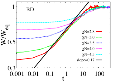
Figure 1: Evolution of the rescaled width $W$ of A/B interfaces in incompatible homopolymer blends as a function of time $t$ (in units of $t_{0}$) in double logarithmic representation, as obtained from BD simulations for different final incompatibility parameters $\chi N$ as indicated. The inital state is an equilibrated interface at $\chi N=8$. The data for $W$ are rescaled with the equilibrium width of the final state. The solid black line indicates an apparent power law $W(t)\propto t^{a}$ with $a\approx 0.17$. The magnitude of the errorbars here is comparable to that shown in Fig.(2).

Fig. 1 shows the evolution of the interfacial width $W$ as a function of time after such a sudden jump from $\chi N=8$ to different smaller values of $\chi N$, as obtained in the BD simulations. The data for $W$ are rescaled by the corresponding final, equilibrated value. Except for early times, the curves for different $\chi N$ parameters collapse onto a single master curve, which follows an apparent scaling relation $W(t)\propto t^{a}$ at intermediate times interface_FH with exponent $a\approx 0.17$.

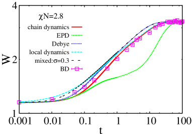
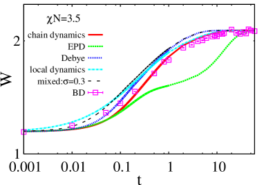
Figure 2: Interfacial width (in units of $R_{g}$) as a function of time (in units of $t_{0}$) in double logarithmic representation, as obtained by different DDF models as indicated (chain dynamics, EPD, Debye dynamics, local dynamics, and mixed dynamics with $\sigma=0.3$), compared to the BD simulation results (symbols), for $\chi N=2.8$ (a) and $\chi N=3.5$ (b). The initial configuration corresponds to an equilibrated interface at $\chi N=8$. The magnitude of errorbars is smaller than the size of the symbols.

Figure 2 compares the predictions for the broadening of the interfacial width from the different DDF models discussed in Sec. III with the BD results for two examples of $\chi N$ jumps. The predictions of the chain dynamics model agree well with the BD simulation results over almost the whole time interval under consideration (except for very early times $t<0.2t_{0}$). The predictions from local dynamics calculations differ slightly, but noticeably from the BD results at early times, and approach them at $t\simeq 4t_{0}$. These results indicate that interfacial broadening is mainly driven by chain diffusion, while the effect of segmental dynamics is minor.

The Debye dynamics calculations reproduce the BD results well at early times, but show small deviations at later times. This is presumably due to the underlying weak inhomogeneity assumption, which is clearly questionable in the presence of sharp interfaces. The mixed model, which is partly based on the Debye model, does not improve on this problem. Overall, however, all DDF predictions discussed so far are acceptable compared to the reference BD simulations; the deviations are quite small. When plotting the DDF predictions for different final $\chi N$ in a similar fashion as in Fig. 1, the data collapse onto a master curve and exhibit the same apparent power law behavior at intermediate times than the BD data, $W(t)\propto t^{a}$ with $a\approx 0.17$ (data not shown).

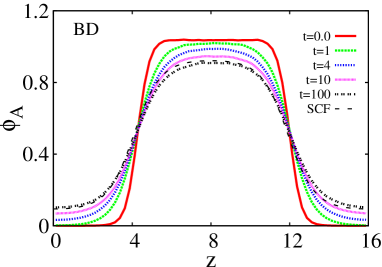
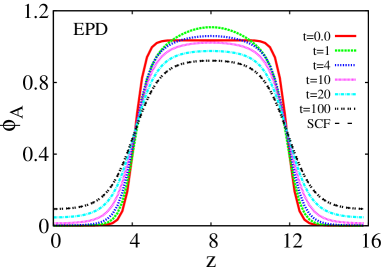
Figure 3: Density profiles of component A obtained in BD simulations (a), and EPD calculations (b) for different times $t$ (in units of $t_{0}$) as indicated. The system is initialized at $\chi N=8$ and then suddenly set to $\chi N=2.8$. The dashed line shows the equilibrium density profile at $\chi N=2.8$ as obtained from self-consistent field (SCF) theory.

This is different for the EPD model. The EPD predictions for the evolution of the interfacial width in Fig. 2 differ strongly from the BD reference data over a wide time window, $0.5t_{0}<t<40t_{0}$. The values for the width are much too small, i.e., the interface broadening is slowed down significantly, and the shape of the curves is very different. To further analyze this problem, we compare in Fig. 3a) and b) the evolution of the A-density profiles obtained from the EPD model with the profiles in the reference BD system. According to the BD simulations (Fig. 3a), A-polymer chains gradually diffuse from the A-polymer rich region to the A-polymer poor region. The amount of A-polymers in the A polymer rich region decreases monotonically with time. The corresponding curves obtained from chain dynamics, local dynamics, Debye, and mixed dynamics calculations are very similar (data not shown). In contrast, the EPD calculation produces a highly unusual, nonmonotonic behavior (Fig. 3b). At intermediate times, A-chains accumulate in the middle of the A-polymer rich slab, such that the A-density there even exceeds the initial value. A shallow peak forms in the middle of the A-slab, which reaches a maximum and then decreases again. The slowdown of interfacial broadening in Fig. 2 is observed precisely in the time range where the peak is highest.

This spurious behavior is only found in the EPD model, and not in the closely related chain dynamics model. It must thus be an artefact of the EPD approximation. If the EPD assumption, $\nabla\Lambda_{\alpha\beta}({\mathbf{r}},{\mathbf{r}}^{\prime})\simeq-\nabla^{\prime}\Lambda_{\alpha\beta}({\mathbf{r}},{\mathbf{r}}^{\prime})$), is not valid, the EPD equations violate local mass conservation, since they no longer have the form of a continuity equation for the densities $\phi_{\alpha}$. Instead, the auxiliary potentials $\omega_{\alpha}$ are locally conserved. Large-scale chain redistributions become possible, which are presumably responsible for the observed artefacts.

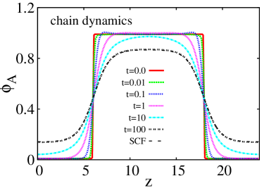
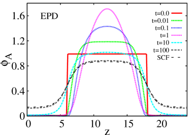
Figure 4: Density profiles of component A obtained from chain dynamics calculations (a), and EPD calculations (b) for different times $t$ (in units of $t_{0}$) as indicated. The system is initialized with two sharp interfaces and then further propagated with $\chi N=2.5$. The dashed line indicates the equilibrium density profile at $\chi N=2.5$ according to the SCF theory.

To further illustrate this problem, we now consider an extreme case where the initial density profile has an almost steplike configuration,

$$\phi_{\mathrm{A}}^{\mathrm{ini}}=\frac{\phi_{\mathrm{min}}+\phi_{\mathrm{max}}}{2}+\frac{\phi_{\mathrm{min}}-\phi_{\mathrm{max}}}{2\tanh(\eta)}\tanh\Big{[}\eta\cos\frac{2\pi}{L_{\mathrm{z}}}z\Big{]}$$ (22)

with $\phi_{\mathrm{min}}=0.01,\phi_{\mathrm{max}}=0.99$, and $\eta=100$. The initial interfacial width is roughly $W\simeq 0.19$. Such unphysical sharp density profiles were also adopted in some other theoretical studies Shi_interface ; interface_poly . Since they cannot easily be generated in particle simulations, we study the evolution of the density profile by DDF methods only. The system size was chosen $L_{\mathrm{z}}=24$ with spatial discretization $\Delta z=0.09R_{g}$ ($n_{\mathrm{z}}=256$ grid points).

Fig. 4 illustrates that the EPD artefacts become even more prominent for such sharp interfaces. The results from the chain dynamics calculations, shown in Fig. 4a, seem quite reasonable. At early times, weak maxima of A-monomer density appear in the A-polymer rich side right next to the interface, which then gradually move away and shrink. A similar phenomenon was reported from DDF studies of interfacial broadening in incompressible polymer blends Shi_interface ; interface_poly . Apart from this overshooting, the evolution of the interfacial density profiles is similar to that shown in Fig. 3a). In contrast, the results from EPD calculations (Fig. 4a) are obviously erroneous. The density of A-chains at the center of the A-slab grows by a factor of almost 2 within a time span of less than $1t_{0}$, which is not compatible with a regular chain diffusion process.

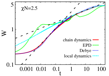
Figure 5: Interfacial broadening with time according to different DDF models as indicated. The initial density profile is a sharp tanh function with width $0.19R_{g}$, and the interaction parameter is $\chi N=2.5$. Dashed lines indicate power laws $W(t)\propto t^{a}$ with exponents $a=0.45$ and $a=0.17$.

Fig. (5) shows the evolution of the interfacial width obtained with different DDF methods for systems that were initialized with the sharp tanh function (22). The results obtained from chain dynamics and Debye dynamics calculations are in good agreement with each other. The curve corresponding to local dynamics differs significantly from the nonlocal schemes at early times and approaches it at later times. Since chain diffusion is a dominant mechanism in interfacial broadening, we expect that the nonlocal schemes reflect the true dynamics more accurately than the local dynamics scheme. The curve produced by the EPD dynamics is rather erratic and has no resemblance to the other curves.

In contrast to Fig. 1, the curves $W(t)$ obtained with the nonlocal schemes (chain dynamics / Debye dynamics) cannot by described by a single scaling law $W(t)\propto t^{a}$. We therefore extract two power law exponents, characterizing the interface broadening at early and later times. At early times, we get $a\approx 0.45$, and at late times $a\approx 0.17$. Experimental studies have also indicated a power law growth of the interfacial width before saturating to the final equilibrium width. The power law exponent reported in the experiments falls between $0.25\sim 0.5$ depending mainly on the annealing temperature blend_E1 ; blend_E2 . Our predicted power law exponent for early times (see Fig 5 matches well with these experimental results. On the other hand, the smaller apparent exponent $a\approx 0.17$ at later times is compatible with the apparent exponent $a\approx 0.17$ extracted from Fig. 1. This is not surprising, as the initial interfaces in Fig. 1 are much wider, and the broadening starts to saturate much earlier.

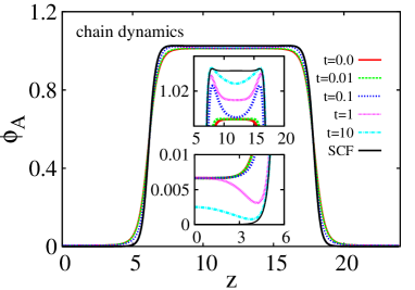
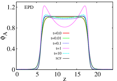
Figure 6: Evolution of A-density profile during interfacial sharpening from an interface corresponding to $\chi N=5$ to an interface corresponding to $\chi N=10$, as obtained by chain dynamics DDF calculations (a) and EPD calculations (b). The Two insets in (a) show blowups of some parts of the curves. “SCF” denotes the equilibrium density profile according to self-consistent field theory at $\chi N=10$.

Now we briefly consider the inverse problem, i.e. interface sharpening after a sudden increase of $\chi N$. We choose as initial density profile the equilibrium density distribution corresponding to $\chi N=5$, then instantaneously quench the system to $\chi N=10$, and monitor the evolution of the density profiles. As in the previous study (Figs. 4, 5), the system has the size $L_{\mathrm{z}}=24$ and is studied with a spatial discretization corresponding to $n_{\mathrm{z}}=256$ grid points. Fig. 6a) shows the density profiles at different times obtained from chain dynamics calculations. In the A-polymer-rich region, the A-density gradually decreases to the final equilibrium value, and in the A-polymer poor region, it gradually increases. Small transient peaks appear close to the interface, but no “overshooting” with respect to the final equilibrium profile is observed. On the other hand, the EPD calculations (Fig. 6b) predict large density overshoots at times around $t\sim 1t_{0}$ and a dramatic transient density reduction at the center of the A-rich slab. These phenomena are obviously again artefacts of the EPD approximation.

We should note that the EPD method has been used to study interfacial broadening in previous work, e.g., by one of us in Ref. interface_poly , and no artefacts were observed. The reason is most likely that these studies considered incompressible blends, where transient large density variations as reported here were not possible. To further analyze the EPD artefacts, we thus systematically study the effect of the Helfand compressibility parameter $\kappa$ on the EPD prediction for the interfacial broadening problem. The parameters and initial conditions are chosen as in Fig.5, i.e., with a sharp initial interface. The Helfand parameter is increased from $\kappa N=10$ to $\kappa N=10.000$. The time step in these simulations has to be reduced with increasing $\kappa N$. Whereas $\Delta t=10^{-3}t_{0}$ is found to be sufficient at $\kappa N=10$ as explained above, we had to use $\Delta t=10^{-6}t_{0}$ at $\kappa N=10.000$.

Figure 7 shows the maximum local density of A-monomers observed during the whole course of a simulation, $\phi_{A}^{\mathrm{max}}$, as a function of the compressibility parameter $\kappa N$. For EPD at $\kappa N=10$, it is almost twice as large as the mean total density $\bar{\phi}=1$ (rescaled), which consistent with the density profile shown in Figure 4 (at $t=1t_{0}$). With increasing $\kappa N$, the maximum density $\phi^{\mathrm{max}}_{\mathrm{A}}$ gradually decreases to reach $\bar{\phi}$ in the infinite large $\kappa N$ limit. As $\kappa N$ approaches infinity, the EPD dynamics becomes similar to that of other DDFT models, i.e., the polymer density in the polymer rich region decreases almost monotonically until it reaches the equilibrium value.

Figure 7 compares the EPD results for the time evolution of the interfacial width for different Helfand parameters $\kappa N$. At $\kappa N=10$, the curve exhibits several oscillations. For larger $\kappa N$, it becomes smoother, but remains nonmonotonic with a spurious peak at early times. With increasing $\kappa N$, the peak becomes smaller and moves to earlier times. For comparison, we also study the strictly incompressible limit $\kappa N\to\infty$ as in Ref.interface_poly (denoted IEPD). As expected, the peak disappears. However, even in this limit, the EPD predictions do not coincide with the results from Debye dynamics or local dynamics calculations (the latter two are found to hardly depend on the compressibility parameter at all). Considering the earlier finding that Debye dynamics calculations reproduce the data from BD simulations nicely in Figure 2 (at $\kappa N=10$), we conclude that the EPD results should probably not be trusted even in the incompressible limit, at least from a quantitative point of view.

We have studied interfacial sharpening (Figure 6) for larger $\kappa N$ (data not shown). Here again, the EPD artefacts disappear at $\kappa N\to\infty$. With increasing $\kappa N$, the spurious maxima in $\phi_{\mathrm{A}}$ gradually decrease and vanish when $\kappa N$ approaches infinity.

We close this subsection with a general remark on the Helfand parameter $\kappa$. It can be seen as a numerical convenience to replace a strictly incompressible system. This is useful in continuum theories where the incompressibility constraint makes the equations very stiff, and it is necessary in particle-based simulations, where maintaining strict incompressibility is close to impossible. In fact, strictly incompressible systems do not exist in nature, even though typical values for the compressibility parameter are of course much higher than $\kappa N=10$. In our DDF calculations, we found the effect of compressibility on the interface broadening dynamics to be negligible in all cases except EPD. Therefore, the popular approach to approximate nearly incompressible blends by compressible blends seems reasonable.

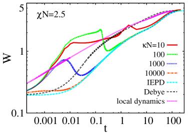
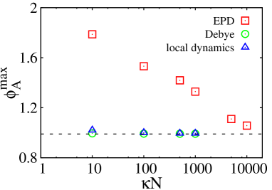
Figure 7: (a) Interfacial broadening with respect to time according to different DDF models and for EPD at different values of the Helfand compressibility parameter $\kappa N$. IEPD refers to EPD in the incompressible limit, $\kappa N\to\infty$. The results for Debye dynamics and local dynamics for different $\kappa\in[10:1000]$ coincide; here we show the curves for $\kappa N=1000$. (b) Maximum density observed during the interfacial broadening process for different DDF models as a function of compressibility parameter $\kappa N$. The dashed line denotes the initial maximum density $\phi_{A}^{\mathrm{initial}}=0.99$. The initial state is chosen as a sharp tanh function as in Figure 5

.

IV.2 Lamellar ordering in a diblock copolymer melt

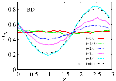
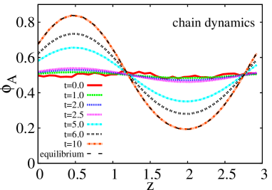
Figure 8: Evolution of density profiles for the A monomers in A:B diblock copolymer melts as obtained from BD simulations (a) and chain dynamics calculations (b). The parameters are chosen $\chi N=12$, $\kappa N=10$, $N_{\mathrm{A}}=N_{\mathrm{B}}$. They start with the same initial conditions. The time is measured in units of $R^{2}_{g}/D_{c}$

Last, we consider the dynamics of microphase separation in initially disordered copolymer melts. Experimentally, this has been studied, e.g., by Floudas and coworkers lamellar_ordering_1 ; lamellar_ordering_2 and by Sakamoto and Hashimoto lamellar_ordering_3 with small angle neutron and X-ray scattering and other methods. These studies focussed on slow processes (time scales of seconds) related to the nucleation and reordering of domains, and fluctuation effects in the vicinity of the order-disorder transition lamellar_ordering_2 . Here we examine the kinetics of local spontaneous ordering after a sudden deep quench into the ordered regime, on time scales of submicroseconds that are hard to resolve experimentally. (For typical polymers, the time scale $t_{0}$ is roughly of the order $10^{-5}$ seconds.)

We consider systems of $n_{\mathrm{c}}$ identical A:B diblock copolymers made of $N$ monomers, where the A block and B block have the same length, i.e. $N_{\mathrm{A}}=N_{\mathrm{B}}$. In all calculations, we set $\chi N=12$, $\kappa N=10$, which lead to a lamellar morphology at equilibrium. We initialize the system by imposing weakly inhomogeneous density distributions, and monitor the evolution of the A-density profile until it is equilibrated. In particular, we consider the evolution of the A-density at the location where it assumes its maximum value (which we denote $\phi_{A}^{\mathrm{max}}$) at the end of the run. The BD simulations are implemented in three dimensional space in systems of size $L_{\mathrm{x}}=L_{\mathrm{y}}=1$, and $L_{\mathrm{z}}=3$ with $n_{\mathrm{x}}\cdot n_{\mathrm{y}}\cdot n_{\mathrm{z}}=10\cdot 10\cdot 40$ uniform cubic cells. The resulting density profiles are homogeneous along the $x$ and $y$ directions and exhibit a lamellar structure with one period in the $z$ direction. We should note that the system is slightly frustrated at equilibrium, as the bulk lamellar spacing is roughly 3.4 $R_{g}$, which is not fully commensurable with the box length $L_{\mathrm{z}}$. Since we are using the same box dimensions in the BD simulations and the DDF calculations, quantitative comparisons are still possible.

Specifically, we studied systems of 5000 chains of length $N=40$. For comparison, we have also considered systems with chain length $N=20$ and $N=60$ at the same mean monomer density (i.e., 10.000 chains and 3000 chains), and obtained similar results (data not shown). The average number of monomers per cell is about 50. The time step in the BD simulations is chosen $\Delta t=0.0003/N$ (i.e., $\Delta t=0.75\cdot 10^{-5}t_{0}$ at $N=40$). The DDF calculations are carried out in one dimension with time step $\Delta t=10^{-4}t_{0}$ in the EPD and Debye dynamics models, $\Delta t=10^{-5}t_{0}$ in the chain dynamics model, and $\Delta t=10^{-6}t_{0}$ in the local dynamics model. We found that such small time steps were necessary in the chain dynamics and local dynamics schemes, otherwise the iterative reconstruction of the auxiliary fields $\omega_{\alpha}$ from the density fields $\phi_{\alpha}$ did not always converge. Adaptive time steps would probably partly relieve these problems.

Fig. 8 shows the density profiles of A-monomers at different times. In the BD simulations, the initial polymer configurations are generated as free Gaussian chains which creates a random density distribution. This distribution, averaged over the $x$ and $y$ directions, is imposed as initial density profile in all DDF schemes. Indeed, we can see from Fig.8a and b that $\phi_{A}(z)$ are the same at $t=0$. As time passes, the system microphase separates into A-rich and B-rich regions and reaches equilibrium at large $t$. The shapes of the equilibrium densities can almost be superimposed after performing a proper translational shift along the abscissa, they therefore represent the same equilibrium state. However, the phase ordering proceeds at different speeds. For example, focussing on the maximum density $\phi_{\mathrm{A}}^{\mathrm{max}}$ at $t=2$, we can see that the BD simulations give $\phi_{\mathrm{A}}^{\mathrm{max}}\simeq 0.59$ at this time (Fig. 8a), while the chain dynamics calculation predicts $\phi_{\mathrm{A}}^{\mathrm{max}}\simeq 0.51$ (Fig. 8b). Hence the ordering in the chain dynamics model is too slow. The curves obtained from other DDF models (including EPD) are qualitatively similar to the BD curves, but the density evolves at different speeds (data not shown).

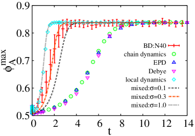
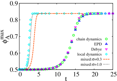
Figure 9: Evolution of $\phi_{A}^{\mathrm{max}}$ with time as obtained from BD simulations and the field-based DDF schemes discussed in this work. In (a), the DDF profiles are initialized to precisely match the initial density distribution in the BD simulations for $N=40$, while in (b), they are initialized by imposing a very small random noise to the initial auxiliary potentials $\omega_{\alpha}({\mathbf{r}})$. (see text for explanation

To further quantify this observation, we now focus on $\phi_{A}^{\mathrm{max}}$. Fig. (9a) compares the evolution of $\phi_{A}^{\mathrm{max}}$ with respect to time obtained from BD simulations with the results of the different DDF models, choosing as initial DDF condition the BD monomer distribution profile at $t=0$. For such “realistic” initial condition, $\phi^{\mathrm{max}}_{\mathrm{A}}\simeq 0.53$ at time $t=0$, indicating that the inhomogeneities in the initial (fully disordered) system are already very high. As time progresses, $\phi^{\mathrm{max}}_{\mathrm{A}}$ first decreases slightly, and then increases continuously until it saturates at the equilibrium value. The predictions from nonlocal chain dynamics models (chain dynamics, Debye dynamics, and EPD) are in good agreement with each other, but they underestimate the rate of ordering. In contrast, the local dynamics model overestimates the ordering velocity. At early times ($t\leq 1$), the local dynamics prediction almost matches the results from the reference BD simulations. Thus the ordering of monomers seems to dominate the dynamics on time scales smaller than the characteristic relaxation time of a chain. At later times, however, the diffusion of the whole chain becomes significant, and large scale correlations begin to play a role. It is then necessary to account for the nonlocal correlations that slow down the dynamics. The density evolution predicted by the pure local dynamics scheme therefore overestimates the rate of ordering at late times.

This problem is addressed by the mixed DDF scheme introduced in Sec. III, Eq. (21). In this scheme, a tunable parameter $\sigma$ is used to control the crossover between local and nonolocal dynamics. On small length scales below $\sigma$, the dynamics is mostly local, whereas on larger scales, it becomes nonlocal. The effect can be seen in Fig. 9a). For $\sigma=1$, the curves calculated with the mixed dynamics reproduce the local dynamics curves. For $\sigma=0.1$, the evolution of $\phi^{\mathrm{max}}_{A}$ is slow and stays on the side of nonlocal dynamics. However, at $\sigma=0.3$, the mixed dynamics approximately reproduces the BD simulation data: If one propagates the motion according to local dynamics on length scales smaller than $0.3R_{g}$, and according to nonlocal dynamics on length scales larger than $0.3R_{g}$, one obtains a dynamical scheme that is quite close to describing the true dynamics. This mixed dynamics scheme accounts for the fact that in the phase ordering process, both the small-scale motion and the large-scale motion are important. The parameter $\sigma$ roughly specifies the weight of these two types of dynamics.

The results of the DDF calculations depend sensitively on the choice of the initial conditions. This is demonstrated in Fig. 9b), which shows that the DDF results if one starts with an almost homogeneous initial density profile decorated with a very weak unphysical noise does not have the correct spatial correlations of a disordered copolymer melt. Specifically, the initial conditions are defined through the initial auxiliary potential fields, which are chosen $\omega_{\alpha\beta}({\mathbf{r}})=0.01\>\xi({\mathbf{r}})$, where $\xi$ are uniformly distributed random numbers in the interval $\xi\in[0:1]$. This results in an initial maximum A-density of $\phi^{\mathrm{max}}_{\mathrm{A}}\approx 0.5002$. The subsequent time evolution of the density profiles is qualitatively similar to that obtained with realistic initial conditions (Fig. 9a): The ordering is much slower in the nonlocal DDF schemes than in the local DDF scheme. The large difference again reflects the multiscale character of the phase ordering process. Most importantly, the comparison with Fig. 9a) shows that the onset of ordering can be delayed significantly if the initial conditions are not chosen appropriately. The problem can presumably be reduced by including thermal noise as described at the end of Sec. III. This has not been done here.

We have also examined the effect of compressibility on the ordering kinetics. We found that increasing $\kappa N$ affects the final density distributions slightly, but it has a negligible effect on the ordering kinetics (data not shown). For example, when examining the maximum density of A monomers, $\phi^{\mathrm{max}}_{\mathrm{A}}$, as a function of time $t$, the curves for different $\kappa N$ (using the same DDF theory) overlap almost completely during the ordering process, but they saturate to different equilibrium values.

V Conclusion and Outlook

The main results of the present work can be summarized as follows: We have compared the predictions of different DDF theories with BD simulations of interface broadening in compressible homopolymer blends and microphase separation in copolymer melts.

• Interface broadening in blends is best described by the nonlocal “chain dynamics” DDF theory.

• DDF calculations based on the Debye approximation do not differ significantly from the full chain dynamics calculations in all situations considered here. In contrast, when looking at interface broadening or sharpening, EPD calculations produce spurious artefacts at intermediate times. The problem becomes worse if the interfaces are sharper. The artefacts disappear in the incompressible limit, however, the EPD results still differ noticeably from those of other DDF theories. This must be attributed to the EPD approximation and is most likely a consequence of the fact that the EPD model does not strictly guarantee local mass conservation.

• Neither local dynamics nor chain dynamics can capture the kinetics of microphase separation in block copolymer melts. Compared to the reference BD simulations, local dynamics calculations underestimate the ordering time, and chain dynamics calculations overestimate it. This most likely reflects the multiscale character of the ordering process, which involves both local chain rearrangements and global chain motions. To address this problem, we have proposed a mixed local/nonlocal DDF scheme, which combines local monomer motion on small scales below $R_{g}$ with global cooperative diffusion on large length scales. This scheme can reproduce the BD simulation results at an almost quantitative level for all situations considered in the present work.

Our mixed DDF approach has some similarity to DDF approaches that have been proposed in the 90s for studying reptation dynamics in strongly entangled polymer systems Kawasaki2 ; Harden . Here, an effective nonlocal Onsager matrix is also constructed such that monomers move differently from whole chains. In the reptation models, the mobility of single monomers is assumed to be reduced compared to whole chains due to their confinement to a tube. Our results here indicate, for the Rouse regime, that it is rather enhanced.

All these DDF schemes have been postulated more or less heuristically. However, our mixed scheme contains one free parameter (the “filter” parameter $\sigma$), which can be used to adjust the DDF calculations to the BD simulations. On the one hand, this reduces the “predictive power” of the approach. On the other hand, it offers a way to incorporate information from more detailed fine-grained models for polymer dynamics in a DDF model in a coarse-grained sense. The parameter $\sigma$ can then be seen as an effective parameter in a dynamic field theory for polymers, which might have to be determined from fine-grained simulations and experiments. In future work, we thus plan to systematically construct mixed schemes from fine-grained simulations, e.g., based on dynamic correlation functions in reference particle simulations. We hope that this approach will help to obtain a more accurate description of polymer dynamics at the field-based level, without the need of explicitly accounting for the multiple time scales involved in polymer relaxation and the corresponding memory effects. Ideally, it should not be restricted to polymers in the Rouse regime, but could also be applied to entangled polymer systems or other complex fluids, and possibly even to nonequilibrium systems under shear stress where polymers are deformed Mueller_Tang .

To summarize, in the present work, we have evaluated different dynamic density functional (DDF) theories for the description of kinetic processes in inhomogeneous polymer systems. As mentioned in the introduction, static density functional theories have proven to be very successful and powerful tools for predicting self-assembled polymeric nanostructures at equilibrium. However, in practice, self-assembly is a nonequilibrium process which often does not run to completion. Polymeric nanostructures are usually not fully equilibrated, and their morphologies and even characteristic length scales may strongly depend on the history of the self-assembly selfassembly ; Simon . This is in fact an advantage, because process design can be used as an additional design principle. However, it also implies that the resulting structures cannot be predicted by static density functional theory alone. We believe that systematic assessments of DDFs such as the one presented here are necessary steps towards an improved theoretical description of nonequilibrium dynamic processes and the resulting nonequilibrium structures.

ACKNOWLEDGMENTS

Financial support from the German Science Foundation (DFG) within project C1 in SFB TRR 146 is gratefully acknowledged. Simulations have been carried out on the computer cluster Mogon at JGU Mainz.

Appendix A Force calculation in BD simulations

In this appendix, we give the explicit expression of the potential force acting on each bead, using the polymer A/B blend as the model system. The simulation box is uniformly divided into $n_{\mathrm{x}}\cdot n_{\mathrm{y}}\cdot n_{\mathrm{z}}$ cells, and densities are defined on the vertexes (mesh points) of these cells. Each cell has a volume of $l_{x}\cdot l_{y}\cdot l_{z}$ (with $l_{I}=L_{I}/n_{I}$). Fractions of a bead are assigned to its neighbouring mesh points according to predefined assignment functions $h(r)$ that depend only on the distance between the particle and the mesh point. Any small displacement of a bead causes a density change, and hence a change of the Hamiltonian. Therefore, the bead experiences a force. In the following, we focus on the (non-bonded) interaction part of the Hamiltonian, and rewrite this part in a discretized form as

$$H_{\mathrm{I}} = \frac{n\chi N}{V}\sum_{g}\Delta V\hat{\phi}_{A}(\mathbf{r}_{g})\hat{\phi}_{B}(\mathbf{r}_{g})$$ (23)

$$+ \frac{n\kappa N}{2V}\sum_{g}\Delta V\big{[}\hat{\phi}_{A}(\mathbf{r}_{g})+\hat{\phi}_{B}(\mathbf{r}_{g})-1\big{]}^{2},$$

where $g$ denotes the index of the mesh point on which the densities are defined, and $\Delta V=l_{x}l_{y}l_{z}$ is the volume of a cell. The densities are calculated using an assignment function, i.e., $\hat{\phi}_{\alpha}(\mathbf{r}_{g})=\frac{1}{\Delta V\rho_{0}}\sum_{j}h(|\mathbf{R}_{j}-\mathbf{r}_{g}|)$ where $\mathbf{R}_{j}$ is the position of the j-th bead, and j runs over all beads of type $\alpha$. We consider the force acting on an A bead at position $\mathbf{R}=(x,y,z)$. The derivative of $H^{(1)}$ with respect to $\mathbf{R}$ can be written as

$$\frac{\partial H_{\mathrm{I}}}{\partial\mathbf{R}} = \frac{\partial h(|\mathbf{R}-\mathbf{r}_{g}|)}{\partial\mathbf{R}}\Big{[}\chi\sum_{g}\hat{\phi}_{B}(\mathbf{r}_{g})$$ (24)

$$+\kappa\sum_{g}\Big{(}\hat{\phi}_{A}(\mathbf{r}_{g}).+\hat{\phi}_{B}(\mathbf{r}_{g})-1\Big{)}\Big{]}$$

In order to proceed, we need to give an explicit expression for the assignment function. For this purpose, we consider the cell where $\mathbf{R}$ is located. The cell has eight vortices at the corners, which we label by indices $i,j,k$ along $x,y,z$ directions, such that the set of indices $i=0,j=0,k=0$ marks the vertex number 0 with coordinate $(0,0,0)$, $i=0,j=0,k=1$ marks the vertex number 1 with coordinate $(0,0,l_{z})$, $i=0,j=1,k=0$ marks the vertex number 2 with coordinate $(0,l_{y},0)$, and so on until $i=1,j=1,k=1$ marks the the vertex number 7 with coordinate $(l_{x},l_{y},l_{z})$. Several choices for the assignment function are conceivable. In the lowest order scheme – the so-called nearest-grid scheme – each bead is fully assigned to its nearest mesh point. Here we use a higher order scheme, which assigns fractions of each bead to its eight nearest mesh points. The fraction assigned to a given vertex is proportional to the volume of a rectangle whose diagonal is the line connecting the particle position and the mesh point on the opposite side of the mesh cell. With the precise arrangement of vortices, the assignment function for each vertex can be written as

$$h(|\mathbf{R}-\mathbf{r}_{g}|)=\frac{(l_{x}-|r_{gx}-x|)(l_{y}-|r_{gy}-y|)(l_{z}-|r_{gz}-z|)}{l_{x}l_{y}l_{z}},$$ (25)

where $g$ ranges from 0 to 7, and $r_{g\alpha}$ is the $\alpha$ component of $\mathbf{r}_{g}$. With these assignment functions, the force from non-bonded interactions acting on an A bead along the $x$ direction is given by

$$-F_{x} = \frac{\partial H_{\mathrm{I}}}{\partial R_{x}}=\frac{1}{N}\frac{\partial u_{A}}{\partial R_{x}}=\frac{u_{A}(\mathbf{r}_{5})-u_{A}(\mathbf{r}_{1})}{Nl_{x}}\frac{(l_{y}-y)z}{l_{y}l_{z}}$$ (26)

$$+ \frac{u_{A}(\mathbf{r}_{6})-u_{A}(\mathbf{r}_{2})}{Nl_{x}}\frac{y(l_{z}-z)}{l_{y}l_{z}}+\frac{u_{A}(\mathbf{r}_{7})-u_{A}(\mathbf{r}_{3})}{Nl_{x}}\frac{yz}{l_{y}l_{z}}$$

$$+ \frac{u_{A}(\mathbf{r}_{4})-u_{A}(\mathbf{r}_{0})}{Nl_{x}}\frac{(l_{y}-y)(l_{z}-z)}{l_{y}l_{z}},$$

the non-bonded force in $y$ direction is

$$-F_{y} = \frac{\partial H_{\mathrm{I}}}{\partial R_{y}}=\frac{1}{N}\frac{\partial u_{A}}{\partial R_{y}}=\frac{u_{A}(\mathbf{r}_{6})-u_{A}(\mathbf{r}_{4})}{Nl_{y}}\frac{x(l_{z}-z)}{l_{z}l_{x}}$$ (27)

$$+ \frac{u_{A}(\mathbf{r}_{3})-u_{A}(\mathbf{r}_{1})}{Nl_{y}}\frac{(l_{x}-x)z}{l_{x}l_{z}}+\frac{u_{A}(\mathbf{r}_{7})-u_{A}(\mathbf{r}_{5})}{Nl_{y}}\frac{zx}{l_{x}l_{z}}$$

$$+ \frac{u_{A}(\mathbf{r}_{2})-u_{A}(\mathbf{r}_{0})}{Nl_{y}}\frac{(l_{x}-x)(l_{z}-z)}{l_{x}l_{z}}$$

and the non-bonded force in $z$ direction is

$$-F_{z} = \frac{\partial H_{\mathrm{I}}}{\partial R_{z}}=\frac{1}{N}\frac{\partial u_{A}}{\partial R_{z}}=\frac{u_{A}(\mathbf{r}_{5})-u_{A}(\mathbf{r}_{4})}{Nl_{z}}\frac{x(l_{y}-y)}{l_{x}l_{y}}$$ (28)

$$+ \frac{u_{A}(\mathbf{r}_{3})-u_{A}(\mathbf{r}_{2})}{Nl_{z}}\frac{(l_{x}-x)y}{l_{x}l_{y}}+\frac{u_{A}(\mathbf{r}_{7})-u_{A}(\mathbf{r}_{6})}{Nl_{z}}\frac{xy}{l_{x}l_{y}}$$

$$+ \frac{u_{A}(\mathbf{r}_{1})-u_{A}(\mathbf{r}_{0})}{Nl_{z}}\frac{(l_{x}-x)(l_{y}-y)}{l_{x}l_{y}}.$$

Here $R_{\mathrm{I}}$ denotes the I-component of $\mathbf{R}$, while $F_{\mathrm{I}}$ is the Ith component of the force $\mathbf{F}$. Similar expressions are obtained for the non-bonded interaction forces acting on B beads.

Appendix B Discussion and Integration of nonlocal DDF equations

In the following, we briefly sketch the derivation of the DDF models introduced in Sec. III and present the numerical method which we use to integrate the chain dynamics equation. We derive the DDF equations of the non-local chain dynamics DDF model following Maurits et al. EPD1997 , at the example of A:B diblock copolymer melts. The extension to other polymer systems is straightforward.

Our system contains $n_{\mathrm{c}}$ diblock copolymers in a volume $V$. Each chain has the length $N=N_{\mathrm{A}}+N_{\mathrm{B}}$, where $N_{\mathrm{A}}$ is the length of block $A$ and $N_{\mathrm{B}}$ the length of block $B$. For convenience, we choose the continuous chain model, where the chain length is scaled to 1, i.e., $1=N_{\mathrm{A}}/N+N_{\mathrm{B}}/N\equiv h_{\mathrm{A}}+h_{\mathrm{B}}$, and we define the sequence function $\tau(s)=A$ for $s<h_{A}$ and $\tau(s)=B$ for $h_{A}<s<1$. The units of length, energy, and time are chosen as in the main text, i.e., we set $k_{B}T\equiv 1$ as the energy unit, and the radius of gyration of a free ideal chain $R_{\mathrm{g}}=a\sqrt{N/6}$ as the length unit ($a$ is the statistical Kuhn length), and measure time in units of the relaxation time of the whole chain, $\tau=R_{g}^{2}/D_{\mathrm{c}}$, where $D_{\mathrm{c}}$ is the diffusion constant of a whole chain.

In the Rouse regime, the internal structure of chains relaxes faster than the coarse-grained collective motion, therefore whole chains are taken to drift with uniform velocity, according to the following equation of motion:

$$\frac{{\mathrm{d}}\mathbf{R}(s,t)}{{\mathrm{d}}t}=N\int_{0}^{1}{\mathrm{d}}s\sum_{{\beta}=A,B}f_{\beta}[\mathbf{R}(s,t)]\>\delta_{\beta,\tau(s)}.$$ (29)

Here $f_{\beta}=-\nabla\tilde{\mu}_{\beta}$ is the thermodynamic force acting on a monomer of type ${\beta}$ (which is determined from the Helmholtz free energy functional (9) via $\tilde{\mu}_{\beta}=\delta F/\delta\phi_{\beta}$), $s$ is the contour variable, and $\mathbf{R}(s,t)$ denotes the conformation of the chain at time $t$. The conformation dependent rescaled density is given by $\hat{\phi}_{\alpha}=\rho^{-1}_{0}N\sum_{m}\int_{0}^{1}{\mathrm{d}}s\delta(\mathbf{r}-\mathbf{R}_{m}(s,t))\delta_{{\alpha},\tau(s)}$, where the index $m$ runs over all $n_{\mathrm{c}}$ copolymers, and $\rho_{0}=n_{\mathrm{c}}N/V$ is the reference density. The evolution equation for the rescaled density can be obtained by taking directly its derivative with respect to time. After taking the ensemble average at both sides, we obtain the dynamical equation

$$\partial_{t}\phi_{\alpha}=\nabla\cdot\int d\mathbf{r}^{\prime}\sum_{\beta}\Big{[}\tilde{\Lambda}^{\mbox{\tiny chain}}_{\alpha\beta}({\mathbf{r}},{\mathbf{r}}^{\prime},t)\nabla^{\prime}\tilde{\mu}_{\beta}({\mathbf{r}}^{\prime})\Big{]}$$ (30)

with $\phi_{\alpha}=\langle\hat{\phi}_{\alpha}\rangle$, where $\langle\cdots\rangle$ refers to the ensemble average. This is exactly Eq. (12), with Onsager coefficients (the correlators) defined as

$$\tilde{\Lambda}^{\mbox{\tiny chain}}_{\alpha\beta}({\mathbf{r}},{\mathbf{r}}^{\prime},t)\equiv\rho_{0}^{-1}n_{\mathrm{c}}N$$ (31)

$$\times\>\int_{0}^{1}{\mathrm{d}}s\int_{0}^{1}{\mathrm{d}}s^{\prime}\Big{\langle}\delta({\mathbf{r}}-\mathbf{R}(s,t))\delta({\mathbf{r}}^{\prime}-\mathbf{R}_{\beta}(s^{\prime},t))\Big{\rangle}$$

$$= -\frac{\delta\phi_{\alpha}({\mathbf{r}},t)}{\delta\omega_{\beta}({\mathbf{r}}^{\prime},t)}.$$

Eq. (30) is used to derive a set of approximate dynamic schemes including the EPD scheme and the Debye scheme. The approximation involved in EPD is translational symmetry, i.e., one assumes $\nabla\tilde{\Lambda}_{\alpha\beta}({\mathbf{r}},{\mathbf{r}}^{\prime})\simeq-\nabla^{\prime}\tilde{\Lambda}_{\alpha\beta}({\mathbf{r}},{\mathbf{r}}^{\prime})$. Employing this assumption and using the chain rule, $\partial_{t}\phi_{\alpha}=\int{\mathrm{d}}{\mathbf{r}}^{\prime}\sum_{\beta}\frac{\delta\phi_{\alpha}}{\delta\omega_{\beta}({\mathbf{r}}^{\prime})}\partial_{t}\omega_{\beta}({\mathbf{r}}^{\prime})$, one can transform the density evolution equation into an equation propagating the “potential fields”

$$\partial_{t}\omega_{\alpha}=-\nabla^{2}\mu_{\alpha}.$$ (32)

Thus the dynamic equations are simplified considerably. They can be integrated conveniently in Fourier space using fast Fourier transform (FFT). One big advantage of the EPD scheme is that the computationally cumbersome inverse determinations of potential fields $\{\omega_{\alpha}\}$ from density fields $\{\phi_{\alpha}\}$ are avoided, since the $\omega_{\alpha}$ are propagated directly.

The Debye scheme is obtained by applying a weak inhomogeneity expansion (random phase approximation, RPA) polymer_book , where the true correlations are replaced by the correlation functions of ideal Gaussian chains, i.e.,

$$\tilde{\Lambda}^{\mbox{\tiny Debye}}_{\alpha\beta}({\mathbf{r}},{\mathbf{r}}^{\prime},t)\simeq g_{\alpha\beta}^{D}({\mathbf{r}}-{\mathbf{r}}^{\prime}),$$ (33)

where $g_{\alpha\beta}^{D}$ is best given in Fourier space ${\mathbf{q}}$ with

$$g_{{\alpha}{\alpha}}^{D}({\mathbf{q}}) = g_{D}(h_{\alpha},x)$$ (34)

$$g_{AB}^{D}({\mathbf{q}}) = \frac{1}{2}\Big{(}g_{D}(1,x)-g_{D}(h_{A},x)-g_{D}(h_{B},x)\Big{)},$$ (35)

with $x=q^{2}R_{g}^{2}$ and the Debye function $g_{D}(h,x)=\frac{2}{x}(hx+{\rm e}^{-hx}-1)$. In the case of A/B homopolymer blends made of $n_{\alpha}$ homopolymers ${\alpha}$, Eqs. (33-35) are replaced by

$$\tilde{\Lambda}^{\mbox{\tiny Debye}}_{{\alpha}{\alpha}}=\frac{n_{\alpha}}{n_{\mathrm{A}}+n_{\mathrm{B}}}\>g_{D}(1,q^{2}R_{g}^{2}),\quad\tilde{\Lambda}^{\mbox{\tiny Debye}}_{AB}\equiv 0.$$ (36)

In the Debye approximation, the DDF equation for the $\alpha$-component can be written in Fourier space as

$$\partial_{t}\phi_{\alpha}=-q^{2}\sum_{\beta}\tilde{\Lambda}^{\mbox{\tiny Debye}}_{\alpha\beta}({\mathbf{q}})\>\tilde{\mu}_{\beta}({\mathbf{q}}),$$ (37)

Finally in this appendix, we will now present our numerical method for propagating the densities according to the full chain dynamics DDF equations, (30) with (31), without further approximations. We first define the auxiliary vector valued field

$${\mathbf{V}}_{\alpha}({\mathbf{r}})=-\int{\mathrm{d}}{\mathbf{r}}^{\prime}\sum_{\beta}\tilde{\Lambda}^{\mbox{\tiny chain}}_{\alpha\beta}({\mathbf{r}},{\mathbf{r}}^{\prime})\nabla^{\prime}_{\beta}\tilde{\mu}_{\beta}({\mathbf{r}}^{\prime}).$$ (38)

Using this intermediate variable, we can rewrite the DDF equation as

$$\partial_{t}\phi_{\alpha}({\mathbf{r}},t)=-\nabla{\mathbf{V}}_{\alpha}({\mathbf{r}},t).$$ (39)

Provided that ${\mathbf{V}}_{\alpha}$ is known, the integration of this equation is straightforward. Thus we are left with the task to evaluate the intermediate field ${\mathbf{V}}_{\alpha}({\mathbf{r}},t)$. To this end, we make use of the relation $\tilde{\Lambda}^{\mbox{\tiny chain}}_{\alpha\beta}({\mathbf{r}},{\mathbf{r}}^{\prime})=-\delta\phi_{\alpha}({\mathbf{r}})/\delta\omega_{\beta}({\mathbf{r}}^{\prime})$ and rewrite Eq. (38) as

$${\mathbf{V}}_{\alpha}({\mathbf{r}}) = \int{\mathrm{d}}{\mathbf{r}}^{\prime}\sum_{\beta}\delta\phi_{\alpha}({\mathbf{r}})/\delta\omega_{\beta}({\mathbf{r}}^{\prime})\nabla^{\prime}_{\beta}\tilde{\mu}_{\beta}({\mathbf{r}}^{\prime})$$ (40)

$$= \nabla_{\mathbf{u}}\phi_{\alpha}[\{\omega_{\beta}+{\mathbf{u}}\cdot\nabla\tilde{\mu}_{\beta}\}]_{{\mathbf{u}}=0},$$

where $\nabla_{\mathbf{u}}$ denotes the gradient operator with respect to ${\mathbf{u}}$. Eqs. (39) and (40) suggest the following Euler forward algorithm for integrating the chain dynamics DDF equations:

1. Find the initial potential $\omega_{\alpha}^{(0)}$ corresponding to the initial density $\phi_{\alpha}^{(0)}$. This is done by numerical iteration methods.

2. Choose a small parameter $\epsilon$, and calculate the components $I=x,y,z$ of ${\mathbf{V}}_{\alpha}$ according to

   $$V_{{\alpha},I}=\frac{1}{\epsilon}\phi_{\alpha}[\{\omega_{\beta}^{(0)}+\epsilon\partial_{I}\tilde{\mu}^{(0)}_{\beta}\}]-\phi_{\alpha}[\{\omega_{\beta}^{(0)}\}],$$ (41)

   where $\tilde{\mu}^{(0)}_{\alpha}$ is an explicit function of $\{\omega_{\beta}^{(0)}\}$ and $\{\phi_{\beta}^{(0)}\}$.

3. Propagate the density over one time step, i.e., evaluate the density at time $t+\Delta t$ using the explicit Euler scheme

   $$\phi_{\alpha}^{(1)}(t+\Delta t)=\phi_{\alpha}^{(0)}(t)-\Delta t\>\nabla\cdot{\mathbf{V}}_{\alpha}.$$ (42)

The above procedure is repeated to obtain the time evolution of the densities as well as the auxiliary potentials. The same idea can be used to construct more sophisticated integration schemes (beyond explicit Euler). Compared to the EPD scheme, the present scheme is more accurate, since it does not rely on the EPD assumption of translational symmetry. However, it requires much more computing time, since it involves the evaluation of all spatial components of ${\mathbf{V}}$ and the iterative reconstruction of the auxiliary potentials from the densities in each time step.

Appendix C Dynamic density functional theory with fluctuations

On the basis of DDFT, fluctuations can be included in Eq. (12) by adding a thermal noise term,

$$\partial_{t}\phi_{\alpha}=\nabla\int{\mathrm{d}}{\mathbf{r}}^{\prime}\tilde{\Lambda}_{\alpha\beta}({\mathbf{r}},{\mathbf{r}}^{\prime})\>\nabla^{\prime}\tilde{\mu}_{\beta}({\mathbf{r}}^{\prime})+\zeta_{\alpha}({\mathbf{r}},t),$$ (43)

i.e., a stochastic Gaussian distributed field $\zeta_{\alpha}({\mathbf{r}},t)$ with zero mean ($\langle\zeta_{\alpha}({\mathbf{r}},t)\rangle=0$), which is correlated according to the fluctuation-dissipation theorem:

$$\langle\zeta_{\alpha}({\mathbf{r}},t)\zeta_{\beta}({\mathbf{r}}^{\prime},t^{\prime})\rangle=-2\frac{V}{n_{\mathrm{c}}}\>\delta(t-t^{\prime})\>\nabla\tilde{\Lambda}_{\alpha\beta}({\mathbf{r}},{\mathbf{r}}^{\prime})\nabla^{\prime}$$ (44)

Equivalently, one can add a fluctuating current,

$$\partial_{t}\phi_{\alpha}=\nabla\Big{(}\int{\mathrm{d}}{\mathbf{r}}^{\prime}\tilde{\Lambda}_{\alpha\beta}({\mathbf{r}},{\mathbf{r}}^{\prime})\>\nabla^{\prime}\tilde{\mu}_{\beta}({\mathbf{r}}^{\prime})+{\mathbf{j}}_{\alpha}\Big{)},$$ (45)

with $\langle{\mathbf{j}}({\mathbf{r}},t)\rangle=0$ and

$$\langle j_{{\alpha}I}({\mathbf{r}},t)j_{{\beta}J}({\mathbf{r}}^{\prime},t^{\prime})\rangle=2\>\frac{V}{n_{\mathrm{c}}}\>\delta(t-t^{\prime})\>\delta_{IJ}\>\tilde{\Lambda}_{\alpha\beta}({\mathbf{r}},{\mathbf{r}}^{\prime}),$$ (46)

where $I,J$ denote Cartesian coordinates. The amplitude of thermal noise is measured by the inverse Ginzburg parameter polymer_book $C^{-1}=k_{B}T\>V/n_{\mathrm{c}}R_{g}^{3}$. If $C^{-1}$ is large (e.g. $C^{-1}\gg 1$), fluctuations are important, and stochastic DDFT descriptions are required.

References

Guo, Q. Polymer Morphology: Principles, Charcterization, and Processing, Wiley, 2016.

Boudenne, A.; Ibos, L., Candau, Y.; Thomas, S. Eds., Handbook of multiphase polymer systems, Wiley, 2011.

Bailey, A. E.; Poon, W. C. K.; Christianson, R. J.; Schofield, A. B.; Gasser, U.; Prasad, V.; Manley, S.; Segre, P. N.; Cipelletti, L.; Meyer, W. V.; Doherty, M. P.; Sankaran, S.; Jankovsky, A. L.; Shiley, W. L.; Bowen, J. P.; Eggers, J. C.; Kurta, C.; Jr. Lorik, T.; Pusey, P. N.; Weitz, D. A. Spinodal decomposition in a model colloid-polymer mixture in microgravity. Phys. Rev. Lett. 2007, 99, 205701.

Béziel, W.; Fragneto, G.; Cousin, F.; Sferrazza, M. Neutron reflectivity study of the kinetics of polymer-polymer interface formation. Phys. Rev. E 2008, 78, 022801.

Pearson, A. J.; Wang, T.; Lidzey, D. G. The role of dynamic measurements in correlating structure with optoelectronic properties in polymer:fullerene bulk-heterojunction solar cells. Rep. Progr. Phys. 2013, 76, 022501.

Zhang, C.; Fan, Y.; Zhang, Y.; Yu, C.; Li, H.; Chen, Y.; Hamley, I. W.; Jiang, S. Self-assembly kinetics of amphiphilic dendritic copolymers. Macromolecules 2017, 50, 1657-1665.

Kawasaki, K.; Sekimoto, K. Dynamical theory of polymer melt morphology. Physica A 1987, 143, 349–413.

Kawasaki, K.; Sekimoto, K. Morphology dynamics of block copolymer systems. Physica A 1988, 148, 361–413.

Harden, J. Kinetics of interface formation between weakly incompatible polymer blends. J. Physique 1990, 51, 1777–1784.

Fraaije, J. G. E. M.; van Vlimmeren, B. A. C.; Maurits, N. M.; Postma, M.; Evers, O. A.; Hoffmann, C.; Altevogt, P.; Goldbeck-Wood, G. The dynamic mean-field density functional method and its application to the mesoscopic dynamics of quenched block copolymer melts. J. Chem. Phys. 1997, 106, 4260-4269.

Maurits, N. M.; Fraaije, J. G. E. M. Mesoscopic dynamics of copolymer melts: from density dynamics to external potential dynamics using nonlocal kinetic coupling. J. Chem. Phys. 1997, 107, 5879-5889

Hasegawa, R.; Doi, M. Adsorption dynamics. Extension of self-consistent field theory to dynamic problems. Macromolecules 1997, 30, 3086-3089.

Kawakatsu, T. Effects of changes in the chain conformations on the kinetics of order-disorder transitions in block copolymer melts. Phys. Rev. E 1997, 56, 3240-3246.

Yeung, C.; Shi, A.-C. Formation of interfaces in incompatible polymer blends: a dynamical mean field study. Macromolecules 1999, 32, 3637-3642.

Shima, T.; Kuni, H.; Okabe, Y.; Doi, M.; Yuan, X.-F.; Kawakatsu, T. Self-consistent field theory of viscoelastic behavior of inhomogeneous dense polymer systems. Macromolecules 2003, 36, 9199–9204.

Müller, M.; Schmid, F. Incorporating fluctuations and dynamics in self-consistent field theory for polymer blends. Adv. Polym. Sci. 2005, 185, 1-58.

He, X.; Schmid, F. Dynamics of spontaneous vesicle formation in dilute solutions of amphiphilic diblock copolymers. Macromolecules 2006, 39, 2654-2662.

Uneyama, T. Density functional simulation of spontaneous formation of vesicle in block copolymer solutions. J. Chem. Phys. 2007, 126, 114902.

Zhang, X.; Qi, S.; Yan, D. Spinodal assisted growing dynamics of critical nucleus in polymer blends. J. Chem. Phys. 2012, 137, 184903.

Chaikin, P. M.; Lubensky, T. C. Principles of condensed matter physics, Cambridge University Press: 1995.

Hohenberg, P. C.; Halperin, B. I. Theory of dynamic critical phenomena. Rev. Mod. Phys. 1977, 49, 436-479.

Ohta, T.; Kawasaki, K. Equilibrium morphology of block copolymer melts. Macromolecules 1986, 19, 2621–2632.

Gomez, L. R.; Garica, N. A.; Vitelli, V.; Lorenzana, J.; Vega, D. Phase nucleation in curved space. Nature Communications 2015, 6, 6856.

Abate, A.; Vu, G.; Pezzutti, A.; Garcia, N.; Davis, R.; Schmid, F.; Register, R.; Vega, D. Shear-aligned block copolymer monolayers as seeds to control the orientational order in cylinder forming block copolymer thin films. Macromolecule 2016, 49, 7588.

Kessler, S.; Schmid, F.; Drese, K. Modeling size controlled nanoparticle precipitation with the co-solvency method by spinodal decomposition. Soft Matter 2016, 12, 7231–7240.

Helfand, E. Theory of inhomogeneous polymers – fundamentals of Gaussian random-walk model. J. Chem. Phys. 1975, 62, 999–1005.

Freed, K.F. Interrelation between density-functional and self-consistent-field formulations for inhomogeneous polymer systems. J. Chem. Phys. 1995, 103, 3230–3239.

Schmid, F. Self-consistent field theories for complex fluids. J. Phys.: Cond. Matter 1998, 10, 8105–8138.

Matsen, M.W. The standard Gaussian model for block copolymer melts. J. Phys.: Cond. Matter 2002, 14, R21-R47.

Schmid, F. Theory and simulation of multiphase polymer systems. in Handbook of multiphase polymer systems Boudenne, A.; Ibos, L., Candau, Y.; Thomas, S. Eds., chapter 3, 31–80, Wiley 2011.

Dean, D. S. Langevin equation for the density of a system of interacting Langevin processes. J. Phys. A: Math. Gen. 1996, 29, L613-L617.

Frusawa, H; Hayakawa, R. On the controversy over the stochastic density functional equations. J. Phys. A: Math. Gen. 2000, 33, L155-L160.

Marconi, U. M. B.; Tarazona, P. Dynamic density functional theory of fluids. J. Chem. Phys. 1999, 110, 8032-8044.

Evans; R, Archer, A. J. Dynamic density functional theory and its application to spinodal decomposition. J. Chem. Phys. 2004, 121, 4246-4254.

Bagchi, B. Stability of supercooled liquid to periodic density waves and dynamics of freezing. Physica A, 1987, 145, 273-289.

Archer, A. J.; Rauscher, M. Dynamic density functional theory for interacting Brownian particles: stochastic or deterministic. J. Phys. A: Math. Gen. 2004, 37, 9325.

Brader, J. M.; Schmidt. M. Power functional theory for the dynamic test particle limit. J. Phys.: Cond. Matter 2015, 27, 194106.

Schmidt, M.; Brader, J. M. Power functional theory for Brownian dynamics. J. Chem. Phys. 2013, 138, 214101.

Marconi, U. M. B.; Tarazona, P. Dynamic density functional theory of fluids. J. Phys.: Condens. Matter 2000, 12, A413-A418.

Fredrickson, G. H.; Orland, H. Dynamics of polymers: a mean-field theory. J. Chem. Phys. 2014, 140, 084902

Grzetic, D. J.; Wickham, R. A.; Shi, A.-C. Statistical dynamics of classical systems: a self-consistent field approach. J. Chem. Phys. 2014, 140, 244907.

Ganesan, V.; Pryamitsyn, V. A. Dynamical mean-field theory for inhomogeneous polymeric systems. J. Chem. Phys. 2003, 118, 4345-4348.

Narayanan, B.; Pryamitsyn, V. A.; Ganesan, V. Interfacial phenomena in polymer blends: a self-consistent Brownian dynamics study. Macromolecules 2004, 37, 10180-10194.

Müller, M.; Smith, G. D. Phase separation in binary mixtures containing polymers: A quantitative comparison of single-chain-in-mean-field simualtions and computer simulations of the corresponding multichain system. J. Polym. Sci., Part B 2005, 43, 934–958.

Daoulas, K. Ch.; Müller, M. Single-chain in mean field simulations: Quasi-instantaneous field approximation and quantitative comparison with Monte Carlo simulations. J. Chem. Phys. 2006, 125, 184904.

Milano, G.; Kawakatsu, T. Hybrid particle-field molecular dynamics simulations for dense polymer systems. J. Chem. Phys. 2009, 130, 214106.

Zwanzig, R. Nonequilibrium statistical mechanics, Oxford University Press, 2001.

Kinjo, T.; Hyodo, S.-A. Equation of motion for coarse-grained simulation base on microscopic description. Phys. Rev. E 2007, 75, 051109.

Hijón, C.; Español, P.; Vanden-Eijnden, E.; Delgado-Buscalioni, R. Mori-Zwanzig formalism as a practical computational tool. Faraday Discuss. 2010, 144, 301-322.

Reister, E.; Müller, M.; Binder, K. Spinodal decomposition in a binary polymer mixture: dynamic self-consistent-field theory and Monte Carlo simulations. Phys. Rev. E 2001, 64, 041804.

Reister, E.; Müller, M. Formation of enrichment layers in thin polymer films: the influence of single chain dynamics. J. Chem. Phys. 2003, 118, 8476-8488

He, X. H.; Schmid, F. Spontaneous formation of complex micelles from homogeneous solution. Phys. Rev. Lett. 2008, 100, 137802.

Qi, S.; Zhang, X.; Yan, D. External potential dynamic studies on the formation of interface in polydisperse polymer blends. J. Chem. Phys. 2010, 132, 064903

Fan, J.J.; Li, W.; Pan, D.; Shi, M. F. External potential dynamics simulations of morphological transitions in diblock copolymer melt under an electric field. Adv. Mater. Res. 2014, 915-916, 545–548.

Raman, V.; Hatton, T. A.; Olsen, B. D. Kinetics of magnetic field-induced orientational ordering in block copolymer / superparamagnetic nanoparticle composites. Macromolecular Rapid Communications 2014, 35, 2005–2011.

Li, W.; Jiang, W. External potential dynamics simulation of the compatibility of T-shaped graft copolymer compatibilizing two immiscible homopolymers. E-polymers 2010, 055

Heuser, J. ; Sevink, G.J.A.; Schmid, F. Self-assembly of polymeric particles in Poiseuille flow: A hybrid Lattice Boltzmann/External Potential Dynamics simulation study. Macromolecules 2017, doi:10.1021/acs.macromol.6b02684.

Qi, S.; Klushin, L. I.; Skvortsov, A. M.; Polotsky, A. A.; Schmid, F. Stimuli-responsive brushes with active minority components: Monte Carlo study an analytical theory. Macromolecules 2015, 48, 3775-3787.

Edwards, S. F. The statistical mechanics of polymers with excluded volume. Proc. Phys. Soc. 1965, 85, 613-624.

Laradji, M.; Guo, H.; Zuckerman, M. J. Off-lattice Monte Carlo simulation of polymer brushes in good solvents. Phys. Rev. E 1994, 49, 3199-3209.

Qi, S.; Behringer, H.; Raasch, T.; Schmid, F. A hybrid particle-continuum resolution method and its application to a homogeneous solution. Eur. Phys. J. Special Topics 2016, 225, 1527-1549.

Birdsall, C. K.; Fuss, D. Clouds-in-Clouds, Clouds-in-Cell Physics for Many-Body Plasma Simulations. J. Comput. Phys. 1997, 135, 141–148.

Leimkuhler, B.; Matthews, C. Robust and efficient configurational molecular sampling via Langevin dynamics. J. Chem. Phys. 2013, 138, 174102.

Besold, G.; Guo, H.; Zuckermann, M. J. Off-lattice Monte Carlo simulation of discrete Edwards model. J. Polym. Sci., Part B: Polym. Phys. 2000, 38, 1053-1068

Detcheverry, F. A.; Kang, H.; Daoulas, K. Ch.; Müller, M.; Nealey, P. F.; de Pablo, J. J. Monte Carlo simulations of a coarse grain model for block copolymers and nanocomposites. Macromolecules 2008, 41, 4989-5001.

Qi, S.; Behringer, H.; Schmid, F. Using field theory to construct hybrid particle-continuum simulation schemes with adaptive resolution for soft matter systems. New. J. Phys. 2013, 15, 125009.

Sevink, G.J.A.; Schmid, F.; Kawakatsu, T.; Milano, G. Combining cell-based hydrodynamics with hybrid particle-field simulations: Efficient and realistic simulation of structuring dynamics. Soft Matter 2017, 13, 1594-1623.

Doi, M.; Edwards, S. F. The theory of polymer dynamics, Clarendon Press, 1988.

Fredrickson, G. H. The equilibrium theory of inhomogeneous polymers, Oxford University Press: 2006.

Ceniceros, H. D.; Fredrickson, G. H. Numerical solution of polymer self-consistent field theory. Multiscale Model. Simul. 2004, 2, 452-474.

Werner, A.; Schmid, F.; Müller, M.; Binder, K. “Intrinsic” profiles and capillary waves at homopolymer interfaces: A Monte Carlo study. Phys. Rev. E 1999, 59, 728-738.

Wang, S.-Q; Shi, Q. Interdiffusion in binary polymer mixtures. Macromolecules 1993, 26, 1091-1096

Chaturvedi, U. K.; Steiner, U.; Zak, O.; Krausch, G.; Klein, J. Interfacial structure in polymer mixtures below the critical point. Phys. Rev. Lett. 1989, 63, 616-619.

Steiner, U.; Krausch, G.; Schatz, G.; Klein, J. Dynamics of mixing between partially miscible polymers. Phys. Rev. Lett. 1990, 64, 1119-1121.

Floudas, G.; Pakula, T.; Fischer, E. W.; Hadjichristidis, N.; Pispas, S. Ordering kinetics in a symmetric diblock copolymer. Acta Polymer. 1994, 45, 176-181.

Floudas, G.; Vlassopoulos, D.; Pitsikalis, M.; Hadjichristidis, N.; Stamm, M. Order-disorder transition and ordering kinetics in binary diblock copolymer mixtures of styrene and isoprene. J. Chem. Phys. 1996, 104, 2083-2088.

Sakamoto, N.; Hashimoto, T. Ordering dynamics of a symmetric Polystyrene-block-polyisoprene. 2. Real-Space Analysis on the Formation of Lamellar Microdomain. Macromolecules 1998, 31, 3815-3823.

Grzybowski, B.A.; Wilmer, C.E.: Kim, J.: Browne, K.P.; Bishop, K.J.M. Self-assembly: From crystals to cells. Soft Matter 2009, 5, 1110-1128.

Keßler, S; Drese, K; Schmid, F. Simulating copolymeric nanoparticle assembly in the co-solvent method: How mixing rates control final particle sizes and morphologies. Polymer 2017, 126, 9-18.

Müller, M.; Tang, J. Alignment of copolymer morphology by planar step elongation during spinodal self-assembly. Phys. Rev. Lett 2015, 115, 228301.