Observation of a Large-scale Anisotropy in the Arrival Directions of Cosmic Rays above 8×10¹⁸ eV
Abstract
Cosmic rays are atomic nuclei arriving from outer space that reach the highest energies observed in nature. Clues to their origin come from studying the distribution of their arrival directions. Using cosmic rays above electron volts, recorded with the Pierre Auger Observatory from a total exposure of 76,800 square kilometers steradian year, we report an anisotropy in the arrival directions. The anisotropy, detected at more than the 5.2 level of significance, can be described by a dipole with an amplitude of % towards right ascension degrees and declination degrees. That direction indicates an extragalactic origin for these ultra-high energy particles.
7(0,-4) Published in Science as DOI: 10.1126/science.aan4338
Particles with energies ranging from below eV up to beyond eV, known as cosmic rays, constantly hit the Earth’s atmosphere. The flux of these particles steeply decreases as their energy increases; for energies above 10 EeV ( eV), the flux is about one particle per km2 per year. The existence of cosmic rays with such ultra-high energies has been known for more than 50 years [1, 2], but the sites and mechanisms of their production remain a mystery. Information about their origin can be obtained from the study of the energy spectrum and the mass composition of cosmic rays. However, the most direct evidence of the location of the progenitors is expected to come from studies of the distribution of their arrival directions. Indications of possible hot spots in arrival directions for cosmic rays with energy above 50 EeV have been reported by the Pierre Auger and Telescope Array Collaborations [3, 4], but the statistical significance of these results is low. We report the observation, significant at a level of more than 5.2, of a large-scale anisotropy in arrival directions of cosmic rays above 8 EeV.
Above eV, cosmic rays entering the atmosphere create cascades of particles (called extensive air-showers) that are sufficiently large to reach the ground. At 10 EeV, an extensive air-shower (hereafter shower) contains particles spread over an area of km2 in a thin disc moving close to the speed of light. The showers contain an electromagnetic component (electrons, positrons and photons) and a muonic component that can be sampled using arrays of particle detectors. Charged particles in the shower also excite nitrogen molecules in the air, producing fluorescence light that can be observed with telescopes during clear nights.
The Pierre Auger Observatory, located near the city of Malargüe, Argentina, at latitude S, is designed to detect showers produced by primary cosmic rays above 0.1 EeV. It is a hybrid system, a combination of an array of particle detectors and a set of telescopes used to detect the fluorescence light. Our analysis is based on data gathered from 1600 water-Cherenkov detectors deployed over an area of 3000 km2 on a hexagonal grid with 1500-m spacing. Each detector contains 12 tonnes of ultrapure water in a cylindrical container, 1.2 m deep and 10 m2 in area, viewed by three 9-inch photomultipliers. A full description of the observatory, together with details of the methods used to reconstruct the arrival directions and energies of events, has been published [5].
It is difficult to locate the sources of cosmic rays, as they are charged particles and thus interact with the magnetic fields in our galaxy and the intergalactic medium that lies between the sources and Earth. They undergo angular deflections with amplitude proportional to their atomic number , to the integral along the trajectory of the magnetic field (orthogonal to the direction of propagation), and to the inverse of their energy . At EeV, the best estimates for the mass of the particles [6] lead to a mean value for between 1.7 and 5. The exact number derived is dependent on extrapolations of hadronic physics, which are poorly understood because they lie well beyond the observations made at the Large Hadron Collider. Magnetic fields are not well constrained by data, but if we adopt recent models of the Galactic magnetic field [7, 8], typical values of the deflections of particles crossing the Galaxy are a few tens of degrees for EeV, depending on the direction considered [9]. Extragalactic magnetic fields may also be relevant for cosmic rays propagating through intergalactic space [10]. However, even if particles from individual sources are strongly deflected, it remains possible that anisotropies in the distribution of their arrival directions will be detectable on large angular scales, provided the sources have a nonuniform spatial distribution or, in the case of a single dominant source, if the cosmic-ray propagation is diffusive [11, 12, 13, 14].
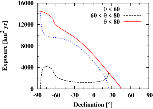
Searches for large-scale anisotropies are conventionally made by looking for nonuniformities in the distribution of events in right ascension [15, 16] because, for arrays of detectors that operate with close to 100% efficiency, the total exposure as a function of this angle is almost constant. The nonuniformity of the detected cosmic-ray flux in declination (fig. S1) imprints a characteristic nonuniformity in the distribution of azimuth angles in the local coordinate system of the array. From this distribution it becomes possible to obtain information on the three components of a dipolar model.
Event observations, selection, and calibration
We analyzed data recorded at the Pierre Auger Observatory between 1 January 2004 and 31 August 2016, from a total exposure of about 76,800 km2 sr year. The 1.2-m depth of the water-Cherenkov detectors enabled us to record events at a useful rate out to large values of the zenith angle, . We selected events with enabling the declination range to be explored, thus covering 85% of the sky. We adopted 4 EeV as the threshold for selection; above that energy, showers falling anywhere on the array are detected with 100% efficiency [17]. The arrival directions of cosmic rays were determined from the relative arrival times of the shower front at each of the triggered detectors; the angular resolution was better than at the energies considered here [5].
Two methods of reconstruction have been used for showers with zenith angles above and below [18, 17]. These have to account for the effects of the geomagnetic field [19, 17] and, in the case of showers with , also for atmospheric effects [20] because systematic modulations to the rates could otherwise be induced (see supplementary materials). The energy estimators for both data sets were calibrated using events detected simultaneously by the water-Cherenkov detectors and the fluorescence telescopes, with a quasi-calorimetric determination of the energy coming from the fluorescence measurements. The statistical uncertainty in the energy determination is 16% above 4 EeV and 12% above 10 EeV, whereas the systematic uncertainty on the absolute energy scale, common to both data sets, is 14% [21]. Evidence that the analyses of the events with and of those with are consistent with each other comes from the energy spectra determined for the two angular bands. The spectra agree within the statistical uncertainties over the energy range of interest [22].
We consider events in two energy ranges, EeV and EeV, as adopted in previous analyses (e.g., [23, 24, 25]). The bin limits follow those chosen previously in [26, 27]. The median energies for these bins are 5.0 EeV and 11.5 EeV, respectively. In earlier work [23, 24, 25], the event selection required that the station with the highest signal be surrounded by six operational detectors—a demanding condition. The number of triggered stations is greater than four for 99.2% of all events above 4 EeV and for 99.9% of events above 8 EeV, making it possible to use events with only five active detectors around the one with the largest signal. With this more relaxed condition, the effective exposure is increased by 18.5%, and the total number of events increases correspondingly from 95,917 to 113,888. The reconstruction accuracy for the additional events is sufficient for our analysis (see supplementary materials and fig. S4).
Rayleigh analysis in right ascension
A standard approach for studying the large-scale anisotropies in the arrival directions of cosmic rays is to perform a harmonic analysis in right ascension, . The first-harmonic Fourier components are given by
| (1) |
The sums run over all detected events, each with right ascension , with the normalization factor . The weights, , are introduced to account for small nonuniformities in the exposure of the array in right ascension and for the effects of a tilt of the array towards the southeast (see supplementary materials). The average tilt between vertical and the normal to the plane on which the detectors are deployed is , so that the effective area of the array is slightly larger for showers arriving from the downhill direction. This introduces a harmonic dependence in azimuth of amplitude to the exposure. The effective aperture of the array is determined every minute. Because the exposure has been accumulated over more than 12 years, the total aperture is modulated by less than as the zenith of the observatory moves in right ascension. Events are weighted by the inverse of the relative exposure to correct these effects (fig. S2).
The amplitude and phase of the first harmonic of the modulation are obtained from
| (2) |
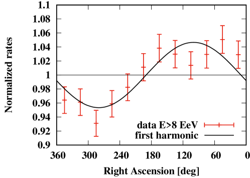
Table 1 shows the harmonic amplitudes and phases for both energy ranges. The statistical uncertainties in the Fourier amplitudes are ; the uncertainties in the amplitude and phase correspond to the 68% confidence level of the marginalized probability distribution functions. The rightmost column shows the probabilities that amplitudes larger than those observed could arise by chance from fluctuations in an isotropic distribution. These probabilities are calculated as [28]. For the lower energy bin ( EeV), the result is consistent with isotropy, with a bound on the harmonic amplitude of at the 95% confidence level. For the events with EeV, the amplitude of the first harmonic is , which has a probability of arising by chance of , equivalent to a two-sided Gaussian significance of 5.6. The evolution of the significance of this signal with time is shown in fig. S3; the dipole became more significant as the exposure increased. Allowing for a penalization factor of 2 to account for the fact that two energy bins were explored, the significance is reduced to 5.4. Further penalization for the four additional lower energy bins examined in [23] has a similarly mild impact on the significance, which falls to 5.2. The maximum of the modulation is at right ascension of . The maximum of the modulation for the EeV bin, at , is compatible with the one determined in the higher-energy bin, although it has high uncertainty and the amplitude is not statistically significant. Table S1 shows that results obtained under the stricter trigger condition and for the additional events gained after relaxing the trigger are entirely consistent with each other.
| Energy [EeV] | Number of events | Fourier coefficient | Fourier coefficient | Amplitude | Phase [∘] | Probability |
| 4 to 8 | 81,701 | 0.60 | ||||
| 32,187 |
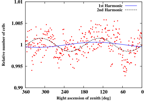
Figure 1 shows the distribution of the normalized rate of events above 8 EeV as a function of right ascension. The sinusoidal function corresponds to the first harmonic; the distribution is compatible with a dipolar modulation: for the first-harmonic curve and for a constant function (where is the number of degrees of freedom, equal to the number of points in the plot minus the number of parameters of the fit).
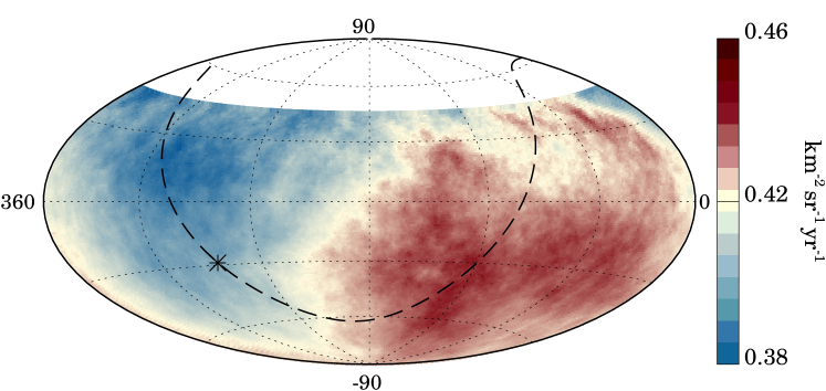
The distribution of events in equatorial coordinates, smoothed with a radius top-hat function to better display the large-scale features, is shown in Fig. 2.
Reconstruction of the three-dimensional dipole
In the presence of a three-dimensional dipole, the Rayleigh analysis in right ascension is sensitive only to its component orthogonal to the rotation axis of Earth, . A dipole component in the direction of the rotation axis of Earth, , induces no modulation of the flux in right ascension, but does so in the azimuthal distribution of the directions of arrival at the array. A non-vanishing value of leads to a sinusoidal modulation in azimuth with a maximum toward the northern or the southern direction.
To recover the three-dimensional dipole, we combine the first-harmonic analysis in right ascension with a similar one in the azimuthal angle , measured counterclockwise from the east. The relevant component, , is given by an expression analogous to that in Eq. 1, but in terms of the azimuth of the arrival direction of the shower rather than in terms of the right ascension. The results are in the EeV bin and in the EeV bin. The probabilities that larger or equal absolute values for arise from an isotropic distribution are 0.8% and 8%, respectively.
Under the assumption that the dominant cosmic-ray anisotropy is dipolar, based on previous studies that found that the effects of higher-order multipoles are not significant in this energy range [25, 29, 30], the dipole components and its direction in equatorial coordinates can be estimated from
| (3) |
[25], where is the mean cosine of the declinations of the events, is the mean sine of the zenith angles of the events, and is the average latitude of the Observatory. For our data set, we find and .
The parameters describing the direction of the three-dimensional dipole are summarized in Table 2. For EeV, the dipole amplitude is , pointing close to the celestial south pole, at , although the amplitude is not statistically significant. For energies above 8 EeV, the total dipole amplitude is , pointing toward . In Galactic coordinates, the direction of this dipole is . This dipolar pattern is clearly seen in the flux map in Fig. 2. To establish whether the departures from a perfect dipole are just statistical fluctuations or indicate the presence of additional structures at smaller angular scales would require at least twice as many events.
| Energy [EeV] | Dipole component | Dipole component | Dipole amplitude | Dipole declination [∘] | Dipole right ascension [∘] |
| 4 to 8 | |||||
| 8 |
Implications for the origin of high-energy cosmic rays
The anisotropy we have found should be seen in the context of related results at lower energies. Above a few PeV, the steepening of the cosmic ray energy spectrum has been interpreted as being due to efficient escape of particles from the Galaxy and/or because of the inability of the sources to accelerate cosmic rays beyond a maximum value of . The origin of the particles remains unknown. Although supernova remnants are often discussed as sources, evidence has been reported for a source in the Galactic center capable of accelerating particles to PeV energies [31]. Diffusive escape from the Galaxy is expected to lead to a dipolar component with a maximum near the Galactic center direction [32]. This is compatible with results obtained in the to eV range [15, 16, 23, 24, 33], which provide values for the phase in right ascension close to that of the Galactic center, .
Models proposing a Galactic origin up to the highest observed energies [34, 35] are in increasing tension with observations. If the Galactic sources postulated to accelerate cosmic rays above EeV energies, such as short gamma-ray bursts or hypernovae, were distributed in the disk of the Galaxy, a dipolar component of anisotropy is predicted with an amplitude that exceeds existing bounds at EeV energies [24, 33]. In this sense, the constraint obtained here on the dipole amplitude (Table 2) for EeV further disfavors a predominantly Galactic origin. This tension could be alleviated if cosmic rays at a few EeV were dominated by heavy nuclei such as iron, but this would be in disagreement with the lighter composition inferred observationally at these energies [6]. The maximum of the flux might be expected to lie close to the Galactic center region, whereas the direction of the three-dimensional dipole determined above 8 EeV lies from the Galactic center. This suggests that the anisotropy observed above 8 EeV is better explained in terms of an extragalactic origin. Above 40 EeV, where the propagation should become less diffusive, there are no indications of anisotropies associated with either the Galactic center or the Galactic plane [36].
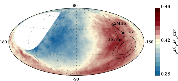
There have been many efforts to interpret the properties of ultrahigh-energy cosmic rays in terms of extragalactic sources. Because of Liouville’s theorem, the distribution of cosmic rays must be anisotropic outside of the Galaxy for an anisotropy to be observed at Earth. An anisotropy cannot arise through deflections of an originally isotropic flux by a magnetic field. One prediction of anisotropy comes from the Compton-Getting effect [37], which results from the proper motion of the Earth in the rest frame of cosmic-ray sources, but the amplitude is expected to be only 0.6% [38], well below what has been observed. Other studies have predicted larger anisotropies. These assume that ultrahigh-energy cosmic rays originate from an inhomogeneous distribution of sources [13, 14, 39], or that they arise from a dominant source and then diffuse through intergalactic magnetic fields [11, 12, 13, 14]. The resulting dipole amplitudes are predicted to grow with energy, reaching 5 to 20% at 10 EeV. These amplitudes depend on the cosmic-ray composition as well as the details of the source distribution. On average, the predictions are smaller for larger source densities or for more isotropically distributed sources. If the sources were distributed like galaxies, the distribution of which has a significant dipolar component [40], a dipolar cosmic-ray anisotropy would be expected in a direction similar to that of the dipole associated with the galaxies. This effect would be due to the excess of cosmic-ray sources in this direction and is different from the Compton-Getting effect due to the Earth’s motion with respect to the rest frame of cosmic rays. For the infrared-detected galaxies in the 2MRS catalogue [40], the flux-weighted dipole points in Galactic coordinates in the direction . In this coordinate system, the dipole we detect for cosmic rays above 8 EeV is in the direction , about away from that of the 2MRS dipole.
For an extragalactic origin, the Galactic magnetic fields modify the direction of the dipole observed at Earth relative to its direction outside the Galaxy. For illustration, Fig. 3 shows a map of the flux above 8 EeV in which the direction of the cosmic-ray dipole is shown along with the direction towards the 2MRS dipole. The arrows in the plot indicate how a dipolar distribution of cosmic rays, in the same direction as the 2MRS dipole outside the Galaxy, would be affected by the Galactic magnetic field [8]. The tips of the arrows indicate the direction of the dipole of the flux arriving at Earth, assuming common values of EeV or 2 EeV. Given the inferred average values for to 5 at 10 EeV, these represent typical values of for the cosmic rays contributing to the observed dipole. The agreement between the directions of the dipoles is improved by adopting these assumptions about the charge composition and the deflections in the Galactic magnetic field. For these directions, the deflections within the Galaxy will also lead to a lowering of the amplitude of the dipole to about 90% and 70% of the original value, for EeV and 2 EeV, respectively. The lower amplitude in the EeV bin might also be the result of stronger magnetic deflections at lower energies.
Our findings constitute the observation of an anisotropy in the arrival direction of cosmic rays with energies above 8 EeV. The anisotropy can be well represented by a dipole with an amplitude of in the direction of right ascension and declination . By comparing our results with phenomenological predictions, we find that the magnitude and direction of the anisotropy support the hypothesis of an extragalactic origin for the highest-energy cosmic rays, rather than sources within the Galaxy.
References and Notes:
- [1] J. Linsley, L. Scarsi, B. Rossi, Phys. Rev. Lett. 6, 485–487 (1961).
- [2] J. Linsley, Phys. Rev. Lett. 10, 146–148 (1963).
- [3] P. Abreu et al., Astropart. Phys. 34, 314–326 (2010).
- [4] Telescope Array Collaboration, Astrophys. J. 790, L21 (2014).
- [5] Pierre Auger Collaboration, Nucl. Instrum. Meth. A 798, 172–213 (2015).
- [6] Pierre Auger Collaboration, Phys. Rev. D 90, 122006 (2014).
- [7] M.S. Pshirkov, P.G. Tinyakov, P.P. Kronberg, K.J. Newton-McGee, Astrophys. J. 738, 192 (2011).
- [8] R. Jansson, G.R. Farrar, Astrophys. J. 757, 14 (2012).
- [9] G.R. Farrar, C. R. Phys. 15, 339–348 (2014).
- [10] R. Durrer, A. Neronov, Astron. Astrophys. Rev. 21, 62 (2013).
- [11] M. Giler, J. Wdowczyk, A.W. Wolfendale, J. Phys. G 6, 1561–1573 (1980).
- [12] V. Berezinsky, S.I. Grigorieva, V.A. Dogiel, Astron. Astrophys. 232, 582 (1990).
- [13] D. Harari, S. Mollerach, E. Roulet, Phys. Rev. D 89, 123001 (2014).
- [14] D. Harari, S. Mollerach, E. Roulet, Phys. Rev. D 92, 063014 (2015).
- [15] IceCube Collaboration, Astrophys. J. 866, 220 (2016).
- [16] KASCADE Collaboration, Nucl. Part. Phys. Proc. 279–281, 56–62 (2016).
- [17] Pierre Auger Collaboration, J. Cosm. Astropart. Phys. 08, 019 (2014).
- [18] Pierre Auger Collaboration, in Proceedings of the 30th International Cosmic Ray Conference, Mérida, Mexico (2007), p. 307.
- [19] Pierre Auger Collaboration, J. Cosm. Astropart. Phys. 11, 022 (2011).
- [20] Pierre Auger Collaboration, J. Instrum. 12, P02006 (2017).
- [21] Pierre Auger Collaboration, in Proceedings, 33rd International Cosmic Ray Conference, Rio de Janeiro (2013), p. 0928.
- [22] Pierre Auger Collaboration, in Proceedings, 34th International Cosmic Ray Conference, The Hague (2015), p. 271.
- [23] Pierre Auger Collaboration, Astropart. Phys. 34, 627–639 (2011).
- [24] Pierre Auger Collaboration, Astrophys. J. 203 (suppl.), 34 (2012).
- [25] Pierre Auger Collaboration, Astrophys. J. 802, 111 (2015).
- [26] N. Hayashida et al., Astropart. Phys. 10, 303–311 (1999).
- [27] D.M. Edge, A.M.T. Pollock, R.J.0. Reid, A.A. Watson, J.G. Wilson, J. Phys. G 4, 133–157 (1978).
- [28] J. Linsley, Phys. Rev. Lett. 34, 1530–1533 (1975).
- [29] Pierre Auger Collaboration, J. Cosm. Astropart. Phys. 06, 026 (2017).
- [30] Pierre Auger and Telescope Array Collaborations, Astrophys. J. 794, 172 (2014).
- [31] HESS collaboration, Nature 531, 476-479 (2016).
- [32] R. Kumar, D. Eichler, Astrophys. J. 781, 47 (2014).
- [33] Pierre Auger Collaboration, Astrophys. J. 762, L13 (2013).
- [34] A. Calvez, A. Kusenko, S. Nagataki, Phys. Rev. Lett. 105, 091101 (2010).
- [35] D. Eichler, N. Globus, R. Kumar, E. Gavish, Astrophys. J. 821, L24 (2016).
- [36] Pierre Auger Collaboration, Astrophys. J. 805, 15 (2015).
- [37] A.H. Compton, I.A. Getting, Phys. Rev. 47, 817–821 (1935).
- [38] M. Kachelrieß, P.D. Serpico, Phys. Lett. B 640, 225–229 (2006).
- [39] P.G. Tinyakov, F.R. Urban, J. Exp. Theor. Phys. 120, 533–540 (2015).
- [40] P. Erdogdu et al., Month. Not. Roy. Astron. Soc. 368, 1515–1526 (2006).
Acknowledgments
The successful installation, commissioning, and operation of the Pierre Auger Observatory would not have been possible without the strong commitment from the technical and administrative staff in Malargüe, and the financial support from a number of funding agencies in the participating countries. The full acknowledgments are in the Supplementary Materials. The Pierre Auger Collaboration will make public the data reproduced in the Figures of this paper on the Auger website on the link to this publication: www.auger.org/data/science2017.tar.gz
Full author list and affiliations
![[Uncaptioned image]](/html/1709.07321/assets/x4.png)
A. Aab63, P. Abreu70, M. Aglietta48,47, I. Al Samarai30, I.F.M. Albuquerque17, I. Allekotte1, A. Almela8,11, J. Alvarez Castillo62, J. Alvarez-Muñiz78, G.A. Anastasi39,41, L. Anchordoqui81, B. Andrada8, S. Andringa70, C. Aramo45, F. Arqueros76, N. Arsene72, H. Asorey1,25, P. Assis70, J. Aublin30, G. Avila9,10, A.M. Badescu73, A. Balaceanu71, F. Barbato54, R.J. Barreira Luz70, J.J. Beatty86, K.H. Becker32, J.A. Bellido12, C. Berat31, M.E. Bertaina56,47, X. Bertou1, P.L. Biermannb, P. Billoir30, J. Biteau29, S.G. Blaess12, A. Blanco70, J. Blazek27, C. Bleve50,43, M. Boháčová27, D. Boncioli41,d, C. Bonifazi23, N. Borodai67, A.M. Botti8,34, J. Brackh, I. Brancus71, T. Bretz36, A. Bridgeman34, F.L. Briechle36, P. Buchholz38, A. Bueno77, S. Buitink63, M. Buscemi52,42, K.S. Caballero-Mora60, L. Caccianiga53, A. Cancio11,8, F. Canfora63, L. Caramete72, R. Caruso52,42, A. Castellina48,47, G. Cataldi43, L. Cazon70, A.G. Chavez61, J.A. Chinellato18, J. Chudoba27, R.W. Clay12, A. Cobos8, R. Colalillo54,45, A. Coleman87, L. Collica47, M.R. Coluccia50,43, R. Conceição70, G. Consolati53, F. Contreras9,10, M.J. Cooper12, S. Coutu87, C.E. Covault79, J. Cronin88, S. D’Amico49,43, B. Daniel18, S. Dasso5,3, K. Daumiller34, B.R. Dawson12, R.M. de Almeida24, S.J. de Jong63,65, G. De Mauro63, J.R.T. de Mello Neto23, I. De Mitri50,43, J. de Oliveira24, V. de Souza16, J. Debatin34, O. Deligny29, C. Di Giulio55,46, A. Di Matteo51,k,41, M.L. Díaz Castro18, F. Diogo70, C. Dobrigkeit18, J.C. D’Olivo62, Q. Dorosti38, R.C. dos Anjos22, M.T. Dova4, A. Dundovic37, J. Ebr27, R. Engel34, M. Erdmann36, M. Erfani38, C.O. Escobarf, J. Espadanal70, A. Etchegoyen8,11, H. Falcke63,66,65, G. Farrar84, A.C. Fauth18, N. Fazzinif, F. Fenu56, B. Fick83, J.M. Figueira8, A. Filipčič74,75, O. Fratu73, M.M. Freire6, T. Fujii88, A. Fuster8,11, R. Gaior30, B. García7, D. Garcia-Pinto76, F. Gatée, H. Gemmeke35, A. Gherghel-Lascu71, P.L. Ghia29, U. Giaccari23, M. Giammarchi44, M. Giller68, D. Głas69, C. Glaser36, G. Golup1, M. Gómez Berisso1, P.F. Gómez Vitale9,10, N. González8,34, A. Gorgi48,47, P. Gorhami, A.F. Grillo41, T.D. Grubb12, F. Guarino54,45, G.P. Guedes19, M.R. Hampel8, P. Hansen4, D. Harari1, T.A. Harrison12, J.L. Hartonh, A. Haungs34, T. Hebbeker36, D. Heck34, P. Heimann38, A.E. Herve33, G.C. Hill12, C. Hojvatf, E. Holt34,8, P. Homola67, J.R. Hörandel63,65, P. Horvath28, M. Hrabovský28, T. Huege34, J. Hulsman8,34, A. Insolia52,42, P.G. Isar72, I. Jandt32, S. Jansen63,65, J.A. Johnsen80, M. Josebachuili8, J. Jurysek27, A. Kääpä32, O. Kambeitz33, K.H. Kampert32, I. Katkov33, B. Keilhauer34, N. Kemmerich17, E. Kemp18, J. Kemp36, R.M. Kieckhafer83, H.O. Klages34, M. Kleifges35, J. Kleinfeller9, R. Krause36, N. Krohm32, D. Kuempel36,32, G. Kukec Mezek75, N. Kunka35, A. Kuotb Awad34, D. LaHurd79, M. Lauscher36, R. Legumina68, M.A. Leigui de Oliveira21, A. Letessier-Selvon30, I. Lhenry-Yvon29, K. Link33, D. Lo Presti52, L. Lopes70, R. López57, A. López Casado78, Q. Luce29, A. Lucero8,11, M. Malacari88, M. Mallamaci53,44, D. Mandat27, P. Mantschf, A.G. Mariazzi4, I.C. Mariş13, G. Marsella50,43, D. Martello50,43, H. Martinez58, O. Martínez Bravo57, J.J. Masías Meza3, H.J. Mathes34, S. Mathys32, J. Matthews82, J.A.J. Matthewsj, G. Matthiae55,46, E. Mayotte32, P.O. Mazurf, C. Medina80, G. Medina-Tanco62, D. Melo8, A. Menshikov35, K.-D. Merenda80, S. Michal28, M.I. Micheletti6, L. Middendorf36, L. Miramonti53,44, B. Mitrica71, D. Mockler33, S. Mollerach1, F. Montanet31, C. Morello48,47, M. Mostafá87, A.L. Müller8,34, G. Müller36, M.A. Muller18,20, S. Müller34,8, R. Mussa47, I. Naranjo1, L. Nellen62, P.H. Nguyen12, M. Niculescu-Oglinzanu71, M. Niechciol38, L. Niemietz32, T. Niggemann36, D. Nitz83, D. Nosek26, V. Novotny26, L. Nožka28, L.A. Núñez25, L. Ochilo38, F. Oikonomou87, A. Olinto88, M. Palatka27, J. Pallotta2, P. Papenbreer32, G. Parente78, A. Parra57, T. Paul85,81, M. Pech27, F. Pedreira78, J. Pȩkala67, R. Pelayo59, J. Peña-Rodriguez25, L. A. S. Pereira18, M. Perlín8, L. Perrone50,43, C. Peters36, S. Petrera39,41, J. Phuntsok87, R. Piegaia3, T. Pierog34, P. Pieroni3, M. Pimenta70, V. Pirronello52,42, M. Platino8, M. Plum36, C. Porowski67, R.R. Prado16, P. Privitera88, M. Prouza27, E.J. Quel2, S. Querchfeld32, S. Quinn79, R. Ramos-Pollan25, J. Rautenberg32, D. Ravignani8, B. Revenue, J. Ridky27, F. Riehn70, M. Risse38, P. Ristori2, V. Rizi51,41, W. Rodrigues de Carvalho17, G. Rodriguez Fernandez55,46, J. Rodriguez Rojo9, D. Rogozin34, M.J. Roncoroni8, M. Roth34, E. Roulet1, A.C. Rovero5, P. Ruehl38, S.J. Saffi12, A. Saftoiu71, F. Salamida51, H. Salazar57, A. Saleh75, F. Salesa Greus87, G. Salina46, F. Sánchez8, P. Sanchez-Lucas77, E.M. Santos17, E. Santos8, F. Sarazin80, R. Sarmento70, C.A. Sarmiento8, R. Sato9, M. Schauer32, V. Scherini43, H. Schieler34, M. Schimp32, D. Schmidt34,8, O. Scholten64,c, P. Schovánek27, F.G. Schröder34, A. Schulz33, J. Schumacher36, S.J. Sciutto4, A. Segreto40,42, M. Settimo30, A. Shadkam82, R.C. Shellard14, G. Sigl37, G. Silli8,34, O. Simag, A. Śmiałkowski68, R. Šmída34, G.R. Snow89, P. Sommers87, S. Sonntag38, J. Sorokin12, R. Squartini9, D. Stanca71, S. Stanič75, J. Stasielak67, P. Stassi31, F. Strafella50,43, F. Suarez8,11, M. Suarez Durán25, T. Sudholz12, T. Suomijärvi29, A.D. Supanitsky5, J. Šupík28, J. Swain85, Z. Szadkowski69, A. Taboada33, O.A. Taborda1, A. Tapia8, V.M. Theodoro18, C. Timmermans65,63, C.J. Todero Peixoto15, L. Tomankova34, B. Tomé70, G. Torralba Elipe78, P. Travnicek27, M. Trini75, R. Ulrich34, M. Unger34, M. Urban36, J.F. Valdés Galicia62, I. Valiño78, L. Valore54,45, G. van Aar63, P. van Bodegom12, A.M. van den Berg64, A. van Vliet63, E. Varela57, B. Vargas Cárdenas62, G. Varneri, R.A. Vázquez78, D. Veberič34, C. Ventura23, I.D. Vergara Quispe4, V. Verzi46, J. Vicha27, L. Villaseñor61, S. Vorobiov75, H. Wahlberg4, O. Wainberg8,11, D. Walz36, A.A. Watsona, M. Weber35, A. Weindl34, L. Wiencke80, H. Wilczyński67, M. Wirtz36, D. Wittkowski32, B. Wundheiler8, L. Yang75, A. Yushkov8, E. Zas78, D. Zavrtanik75,74, M. Zavrtanik74,75, A. Zepeda58, B. Zimmermann35, M. Ziolkowski38, Z. Zong29, F. Zuccarello52,42
- 1
-
Centro Atómico Bariloche and Instituto Balseiro (CNEA-UNCuyo-CONICET), San Carlos de Bariloche, Argentina
- 2
-
Centro de Investigaciones en Láseres y Aplicaciones, CITEDEF and CONICET, Villa Martelli, Argentina
- 3
-
Departamento de Física and Departamento de Ciencias de la Atmósfera y los Océanos, FCEyN, Universidad de Buenos Aires and CONICET, Buenos Aires, Argentina
- 4
-
IFLP, Universidad Nacional de La Plata and CONICET, La Plata, Argentina
- 5
-
Instituto de Astronomía y Física del Espacio (IAFE, CONICET-UBA), Buenos Aires, Argentina
- 6
-
Instituto de Física de Rosario (IFIR) – CONICET/U.N.R. and Facultad de Ciencias Bioquímicas y Farmacéuticas U.N.R., Rosario, Argentina
- 7
-
Instituto de Tecnologías en Detección y Astropartículas (CNEA, CONICET, UNSAM), and Universidad Tecnológica Nacional – Facultad Regional Mendoza (CONICET/CNEA), Mendoza, Argentina
- 8
-
Instituto de Tecnologías en Detección y Astropartículas (CNEA, CONICET, UNSAM), Buenos Aires, Argentina
- 9
-
Observatorio Pierre Auger, Malargüe, Argentina
- 10
-
Observatorio Pierre Auger and Comisión Nacional de Energía Atómica, Malargüe, Argentina
- 11
-
Universidad Tecnológica Nacional – Facultad Regional Buenos Aires, Buenos Aires, Argentina
- 12
-
University of Adelaide, Adelaide, S.A., Australia
- 13
-
Université Libre de Bruxelles (ULB), Brussels, Belgium
- 14
-
Centro Brasileiro de Pesquisas Fisicas, Rio de Janeiro, RJ, Brazil
- 15
-
Universidade de São Paulo, Escola de Engenharia de Lorena, Lorena, SP, Brazil
- 16
-
Universidade de São Paulo, Instituto de Física de São Carlos, São Carlos, SP, Brazil
- 17
-
Universidade de São Paulo, Instituto de Física, São Paulo, SP, Brazil
- 18
-
Universidade Estadual de Campinas, IFGW, Campinas, SP, Brazil
- 19
-
Universidade Estadual de Feira de Santana, Feira de Santana, Brazil
- 20
-
Universidade Federal de Pelotas, Pelotas, RS, Brazil
- 21
-
Universidade Federal do ABC, Santo André, SP, Brazil
- 22
-
Universidade Federal do Paraná, Setor Palotina, Palotina, Brazil
- 23
-
Universidade Federal do Rio de Janeiro, Instituto de Física, Rio de Janeiro, RJ, Brazil
- 24
-
Universidade Federal Fluminense, EEIMVR, Volta Redonda, RJ, Brazil
- 25
-
Universidad Industrial de Santander, Bucaramanga, Colombia
- 26
-
Charles University, Faculty of Mathematics and Physics, Institute of Particle and Nuclear Physics, Prague, Czech Republic
- 27
-
Institute of Physics of the Czech Academy of Sciences, Prague, Czech Republic
- 28
-
Palacky University, RCPTM, Olomouc, Czech Republic
- 29
-
Institut de Physique Nucléaire d’Orsay (IPNO), Université Paris-Sud, Univ. Paris/Saclay, CNRS-IN2P3, Orsay, France
- 30
-
Laboratoire de Physique Nucléaire et de Hautes Energies (LPNHE), Universités Paris 6 et Paris 7, CNRS-IN2P3, Paris, France
- 31
-
Laboratoire de Physique Subatomique et de Cosmologie (LPSC), Université Grenoble-Alpes, CNRS/IN2P3, Grenoble, France
- 32
-
Bergische Universität Wuppertal, Department of Physics, Wuppertal, Germany
- 33
-
Karlsruhe Institute of Technology, Institut für Experimentelle Kernphysik (IEKP), Karlsruhe, Germany
- 34
-
Karlsruhe Institute of Technology, Institut für Kernphysik, Karlsruhe, Germany
- 35
-
Karlsruhe Institute of Technology, Institut für Prozessdatenverarbeitung und Elektronik, Karlsruhe, Germany
- 36
-
RWTH Aachen University, III. Physikalisches Institut A, Aachen, Germany
- 37
-
Universität Hamburg, II. Institut für Theoretische Physik, Hamburg, Germany
- 38
-
Universität Siegen, Fachbereich 7 Physik – Experimentelle Teilchenphysik, Siegen, Germany
- 39
-
Gran Sasso Science Institute (INFN), L’Aquila, Italy
- 40
-
INAF – Istituto di Astrofisica Spaziale e Fisica Cosmica di Palermo, Palermo, Italy
- 41
-
INFN Laboratori Nazionali del Gran Sasso, Assergi (L’Aquila), Italy
- 42
-
INFN, Sezione di Catania, Catania, Italy
- 43
-
INFN, Sezione di Lecce, Lecce, Italy
- 44
-
INFN, Sezione di Milano, Milano, Italy
- 45
-
INFN, Sezione di Napoli, Napoli, Italy
- 46
-
INFN, Sezione di Roma ”Tor Vergata”, Roma, Italy
- 47
-
INFN, Sezione di Torino, Torino, Italy
- 48
-
Osservatorio Astrofisico di Torino (INAF), Torino, Italy
- 49
-
Università del Salento, Dipartimento di Ingegneria, Lecce, Italy
- 50
-
Università del Salento, Dipartimento di Matematica e Fisica “E. De Giorgi”, Lecce, Italy
- 51
-
Università dell’Aquila, Dipartimento di Scienze Fisiche e Chimiche, L’Aquila, Italy
- 52
-
Università di Catania, Dipartimento di Fisica e Astronomia, Catania, Italy
- 53
-
Università di Milano, Dipartimento di Fisica, Milano, Italy
- 54
-
Università di Napoli ”Federico II”, Dipartimento di Fisica “Ettore Pancini“, Napoli, Italy
- 55
-
Università di Roma “Tor Vergata”, Dipartimento di Fisica, Roma, Italy
- 56
-
Università Torino, Dipartimento di Fisica, Torino, Italy
- 57
-
Benemérita Universidad Autónoma de Puebla, Puebla, México
- 58
-
Centro de Investigación y de Estudios Avanzados del IPN (CINVESTAV), México, D.F., México
- 59
-
Unidad Profesional Interdisciplinaria en Ingeniería y Tecnologías Avanzadas del Instituto Politécnico Nacional (UPIITA-IPN), México, D.F., México
- 60
-
Universidad Autónoma de Chiapas, Tuxtla Gutiérrez, Chiapas, México
- 61
-
Universidad Michoacana de San Nicolás de Hidalgo, Morelia, Michoacán, México
- 62
-
Universidad Nacional Autónoma de México, México, D.F., México
- 63
-
IMAPP, Radboud University Nijmegen, Nijmegen, The Netherlands
- 64
-
KVI – Center for Advanced Radiation Technology, University of Groningen, Groningen, The Netherlands
- 65
-
Nationaal Instituut voor Kernfysica en Hoge Energie Fysica (NIKHEF), Science Park, Amsterdam, The Netherlands
- 66
-
Stichting Astronomisch Onderzoek in Nederland (ASTRON), Dwingeloo, The Netherlands
- 67
-
Institute of Nuclear Physics PAN, Krakow, Poland
- 68
-
University of Łódź, Faculty of Astrophysics, Łódź, Poland
- 69
-
University of Łódź, Faculty of High-Energy Astrophysics,Łódź, Poland
- 70
-
Laboratório de Instrumentação e Física Experimental de Partículas – LIP and Instituto Superior Técnico – IST, Universidade de Lisboa – UL, Lisboa, Portugal
- 71
-
“Horia Hulubei” National Institute for Physics and Nuclear Engineering, Bucharest-Magurele, Romania
- 72
-
Institute of Space Science, Bucharest-Magurele, Romania
- 73
-
University Politehnica of Bucharest, Bucharest, Romania
- 74
-
Experimental Particle Physics Department, J. Stefan Institute, Ljubljana, Slovenia
- 75
-
Laboratory for Astroparticle Physics, University of Nova Gorica, Nova Gorica, Slovenia
- 76
-
Universidad Complutense de Madrid, Madrid, Spain
- 77
-
Universidad de Granada and C.A.F.P.E., Granada, Spain
- 78
-
Universidad de Santiago de Compostela, Santiago de Compostela, Spain
- 79
-
Case Western Reserve University, Cleveland, OH, USA
- 80
-
Colorado School of Mines, Golden, CO, USA
- 81
-
Department of Physics and Astronomy, Lehman College, City University of New York, Bronx, NY, USA
- 82
-
Louisiana State University, Baton Rouge, LA, USA
- 83
-
Michigan Technological University, Houghton, MI, USA
- 84
-
New York University, New York, NY, USA
- 85
-
Northeastern University, Boston, MA, USA
- 86
-
Ohio State University, Columbus, OH, USA
- 87
-
Pennsylvania State University, University Park, PA, USA
- 88
-
University of Chicago, Enrico Fermi Institute, Chicago, IL, USA
- 89
-
University of Nebraska, Lincoln, NE, USA
-
—–
- a
-
School of Physics and Astronomy, University of Leeds, Leeds, United Kingdom
- b
-
Max-Planck-Institut für Radioastronomie, Bonn, Germany
- c
-
also at Vrije Universiteit Brussels, Brussels, Belgium
- d
-
now at Deutsches Elektronen-Synchrotron (DESY), Zeuthen, Germany
- e
-
SUBATECH, École des Mines de Nantes, CNRS-IN2P3, Université de Nantes, France
- f
-
Fermi National Accelerator Laboratory, USA
- g
-
University of Bucharest, Physics Department, Bucharest, Romania
- h
-
Colorado State University, Fort Collins, CO
- i
-
University of Hawaii, Honolulu, HI, USA
- j
-
University of New Mexico, Albuquerque, NM, USA
- k
-
now at Université Libre de Bruxelles (ULB), Brussels, Belgium
Acknowledgments
The successful installation, commissioning, and operation of the Pierre Auger Observatory would not have been possible without the strong commitment and effort from the technical and administrative staff in Malargüe.
We are very grateful to the following agencies and organizations for financial support: Argentina – Comisión Nacional de Energía Atómica; Agencia Nacional de Promoción Científica y Tecnológica (ANPCyT); Consejo Nacional de Investigaciones Científicas y Técnicas (CONICET); Gobierno de la Provincia de Mendoza; Municipalidad de Malargüe; NDM Holdings and Valle Las Leñas; in gratitude for their continuing cooperation over land access; Australia – the Australian Research Council; Brazil – Conselho Nacional de Desenvolvimento Científico e Tecnológico (CNPq); Financiadora de Estudos e Projetos (FINEP); Fundação de Amparo à Pesquisa do Estado de Rio de Janeiro (FAPERJ); São Paulo Research Foundation (FAPESP) Grants No. 2010/07359-6 and No. 1999/05404-3; Ministério de Ciência e Tecnologia (MCT); Czech Republic – Grant No. MSMT CR LG15014, LO1305, LM2015038 and CZ.02.1.01/0.0/0.0/16_013/0001402; France – Centre de Calcul IN2P3/CNRS; Centre National de la Recherche Scientifique (CNRS); Conseil Régional Ile-de-France; Département Physique Nucléaire et Corpusculaire (PNC-IN2P3/CNRS); Département Sciences de l’Univers (SDU-INSU/CNRS); Institut Lagrange de Paris (ILP) Grant No. LABEX ANR-10-LABX-63 within the Investissements d’Avenir Programme Grant No. ANR-11-IDEX-0004-02; Germany – Bundesministerium für Bildung und Forschung (BMBF); Deutsche Forschungsgemeinschaft (DFG); Finanzministerium Baden-Württemberg; Helmholtz Alliance for Astroparticle Physics (HAP); Helmholtz-Gemeinschaft Deutscher Forschungszentren (HGF); Ministerium für Innovation, Wissenschaft und Forschung des Landes Nordrhein-Westfalen; Ministerium für Wissenschaft, Forschung und Kunst des Landes Baden-Württemberg; Italy – Istituto Nazionale di Fisica Nucleare (INFN); Istituto Nazionale di Astrofisica (INAF); Ministero dell’Istruzione, dell’Universitá e della Ricerca (MIUR); CETEMPS Center of Excellence; Ministero degli Affari Esteri (MAE); Mexico – Consejo Nacional de Ciencia y Tecnología (CONACYT) No. 167733; Universidad Nacional Autónoma de México (UNAM); PAPIIT DGAPA-UNAM; The Netherlands – Ministerie van Onderwijs, Cultuur en Wetenschap; Nederlandse Organisatie voor Wetenschappelijk Onderzoek (NWO); Stichting voor Fundamenteel Onderzoek der Materie (FOM); Poland – National Centre for Research and Development, Grants No. ERA-NET-ASPERA/01/11 and No. ERA-NET-ASPERA/02/11; National Science Centre, Grants No. 2013/08/M/ST9/00322, No. 2013/08/M/ST9/00728 and No. HARMONIA 5–2013/10/M/ST9/00062, UMO-2016/22/M/ST9/00198; Portugal – Portuguese national funds and FEDER funds within Programa Operacional Factores de Competitividade through Fundação para a Ciência e a Tecnologia (COMPETE); Romania – Romanian Authority for Scientific Research ANCS; CNDI-UEFISCDI partnership projects Grants No. 20/2012 and No.194/2012 and PN 16 42 01 02; Slovenia – Slovenian Research Agency; Spain – Comunidad de Madrid; Fondo Europeo de Desarrollo Regional (FEDER) funds; Ministerio de Economía y Competitividad; Xunta de Galicia; European Community 7th Framework Program Grant No. FP7-PEOPLE-2012-IEF-328826; USA – Department of Energy, Contracts No. DE-AC02-07CH11359, No. DE-FR02-04ER41300, No. DE-FG02-99ER41107 and No. DE-SC0011689; National Science Foundation, Grant No. 0450696; The Grainger Foundation; Marie Curie-IRSES/EPLANET; European Particle Physics Latin American Network; European Union 7th Framework Program, Grant No. PIRSES-2009-GA-246806; European Union’s Horizon 2020 research and innovation programme (Grant No. 646623); and UNESCO.
Supplementary Material
Materials and Methods
Event weights
The Fourier harmonic analysis we perform accounts for modulations in the exposure (of instrumental origin) as well as the effects due to the tilt of the surface detector array. To achieve this each event is weighted by a factor
| (S1) |
where and are the zenith and azimuth angles of the events and is the right ascension directly above the array at the time the -th event was detected. The term enclosed by the round brackets accounts for the effects of the slight tilt of the array. The average inclination from the vertical is , in the direction , i.e. South of the Easterly direction. The tilt term affects only the Fourier analysis in azimuth, and thus the dipole component . The second term in Eq. (S1), , allows for the fact that the effective aperture of the observatory is not uniform in sidereal time. This factor corresponds to the relative number of detector cells, i.e. the active detectors surrounded by at least five other active detectors, present when the right ascension of the zenith of the observatory equals within binning accuracy. It is obtained by adding the number of cells over the whole period of observations, with dead times due to power failures or to communication or acquisition problems discarded. The total number of cells within each bin is normalized to the average value [22]. is plotted in Fig. S2 with a bin width of . This term affects only the Fourier analysis in right ascension, and thus the dipole component . After more than 12 years of continuous operation of the observatory the normalized number of cells shows variations that are smaller than . If the effects of the modulation in the number of cells were not taken into account through the weights, a spurious contribution to of amplitude 0.05% in the direction would be induced. This contribution is an order of magnitude smaller than the statistical uncertainty in the determination of this dipole component, having then a marginal effect. If the effects of the tilt were not taken into account, a spurious contribution to of would be induced. Had we not introduced weighting to the Fourier analysis we would have obtained: for EeV, a total dipole amplitude at with corresponding values for EeV of at .
Energy reconstruction
Two methods of reconstruction have been used for showers with zenith angles above and below [16, 17]. The energy estimator used for showers with is the signal reconstructed at 1000 m from the shower core. This signal is corrected for atmospheric effects [18] that would otherwise introduce systematic modulations to the rates as a function of time of day or season. This could result in spurious influences on the distribution in sidereal time (a time scale that is based on the Earth’s rate of rotation measured relative to the fixed stars rather than the Sun, corresponding to 366.25 cycles/year) and hence could be a source of systematic effects for the anisotropies inferred. The atmospheric effects arise from the dependences of the longitudinal and lateral attenuation of the electromagnetic component of air showers on atmospheric conditions, in particular temperature and pressure. If not corrected, these could cause a modulation of the rates of up to in solar time. The energy estimator is also corrected for geomagnetic effects [19] as otherwise a systematic modulation of amplitude would be induced in the azimuthal distributions.
The particles arriving at the ground in showers with are predominantly muons. As the atmospheric thickness traversed by a shower is proportional to , at those zenith angles the electromagnetic component is almost completely absorbed so that atmospheric effects are negligible. For these large angles the energy estimator is based on the muon content relative to that in a simulated proton-shower of 10 EeV, with the geomagnetic deflections of muons accounted for in the reconstruction of these events [17].
After applying the corrections to those events with , the amplitude of modulation in solar time (365.25 cycles/year) for the whole data set (with and EeV) is reduced to . This is obtained from the first harmonic Fourier analysis of the arrival times as a function of the hour of the day. The residual effect in right ascension, after averaging over more than 12 years, is less than one part in a thousand. As a further check, the amplitude of modulation at the anti-sidereal frequency (364.25 cycles/year) is , consistent with the absence of residual systematic effects. The results of the solar and anti-sidereal amplitudes in the two separate energy bins are also consistent with the absence of systematic effects, being, for EeV of in solar and of in anti-sidereal, while for EeV they are in solar and of in anti-sidereal.
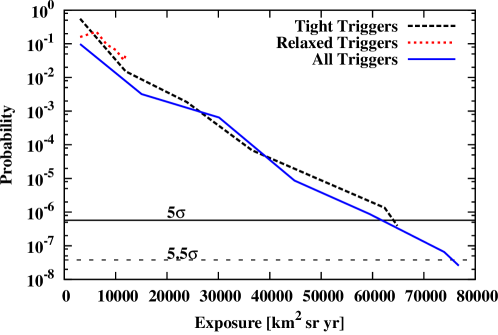
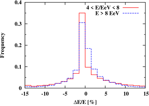
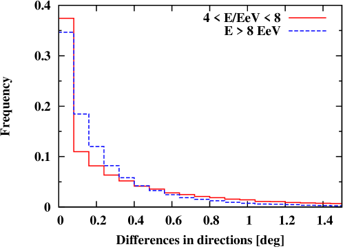
Accuracy of the reconstruction of events obtained with relaxed trigger
Taking events passing the stricter cuts (with six active detectors surrounding the one with the highest signal) and re-analyzing them after removing one of the six detectors, we find that for EeV ( EeV) the difference between the reconstructed directions has an average of (), with 90% of the events having an angular difference smaller than (). The energy estimates differ on average by only 0.2% (0.3%), with a dispersion of (8%). These differences are well below the experimental uncertainties of these two parameters. The distribution of the differences in arrival directions and reconstructed energies between the original event satisfying the strict trigger and those with a missing detector around the one with the highest signal are shown in fig. S4. Events passing the stricter cut from two years of data (2013 and 2014) were analyzed, leading to a total of artificial events passing the relaxed trigger of 65,000 for EeV and 27,000 for ,EeV.
| Dataset | Energy [EeV] | Number of events | Fourier coefficient | Fourier coefficient | Amplitude | Phase [∘] | Probability |
| Tight Triggers | 4 to 8 | 68,775 | 0.007 | 0.44 | |||
| 27,142 | 0.047 | ||||||
| Relaxed Triggers | 4 to 8 | 12,926 | 0.019 | 0.28 | |||
| 5,045 | 0.049 | 0.047 | |||||
| All Triggers | 4 to 8 | 81,701 | 0.005 | 0.60 | |||
| 32,187 | 0.047 |