Predicting Positive and Negative Links with Noisy Queries:
Theory & Practice

Abstract

Social networks involve both positive and negative relationships, which can be captured in signed graphs. The edge sign prediction problem aims to predict whether an interaction between a pair of nodes will be positive or negative. We provide theoretical results for this problem that motivate natural improvements to recent heuristics.

The edge sign prediction problem is related to correlation clustering; a positive relationship means being in the same cluster. We consider the following model for two clusters: we are allowed to query any pair of nodes whether they belong to the same cluster or not, but the answer to the query is corrupted with some probability $0<q<\frac{1}{2}$. Let $\delta=1-2q$ be the bias. We provide an algorithm that recovers all signs correctly with high probability in the presence of noise with $O(\frac{n\log n}{\delta^{2}}+\frac{\log^{2}n}{\delta^{6}})$ queries. This is the best known result for this problem for all but tiny $\delta$, improving on the recent work of Mazumdar and Saha [27]. We also provide an algorithm that performs $O(\frac{n\log n}{\delta^{4}})$ queries, and uses breadth first search as its main algorithmic primitive. While both the running time and the number of queries for this algorithm are sub-optimal, our result relies on novel theoretical techniques, and naturally suggests the use of edge-disjoint paths as a feature for predicting signs in online social networks. Correspondingly, we experiment with using edge disjoint $s-t$ paths of short length as a feature for predicting the sign of edge $(s,t)$ in real-world signed networks. Empirical findings suggest that the use of such paths improves the classification accuracy, especially for pairs of nodes with no common neighbors.

1 Introduction

With the rise of social media, where both positive and negative interactions take place, signed graphs, whose study was initiated by Heider, Cartwright, and Harary [8, 19, 18], have become prevalent in graph mining. A key graph mining problem is the edge sign prediction problem, that aims to predict whether an interaction between a pair of nodes will be positive or negative [22, 23]. Recent works have developed numerous heuristics for this task that perform relatively well in practice [22, 23].

In this work we propose a theoretical model for the edge sign prediction problem that is inspired by active learning [34], and the famous balance theory: “the friend of my enemy is my enemy”, or “the enemy of my enemy is my friend” [8, 15, 19, 36]. Specifically, we model the edge sign prediction problem as a noisy correlation clustering problem [5, 25, 24], where we are able to query a pair of nodes $(u,v)$ to test whether they belong to the same cluster (edge sign $+1$) or not (edge sign $-1$). The query fails to return the correct answer with some probability $0<q<\frac{1}{2}$. Correlation clustering is a basic data mining primitive with a large number of applications ranging from social network analysis [18, 22] to computational biology [20]. The details of our model follow.

Model. Let $V=[n]$ be the set of $n$ items that belong to two clusters. Set $\sigma:V\rightarrow\{-1,+1\}$, and let $R=\{v\in V(G):\sigma(v)=-1\}$ and $B=\{v\in V(G):\sigma(v)=+1\}$ be the sets/groups of red and blue nodes respectively, where $0\leq|R|\leq n$. For any pair of nodes $\{u,v\}$ define $\tau(u,v)=\sigma(u)\sigma(v)\in\{\pm 1\}$ (i.e., $\tau(u,v)=-1$, if $u$ is reported to be in the different cluster than $v$). The coloring function $\sigma$ is unknown and we wish to recover the two sets $R,B$ by querying pairs of items. (We need not recover the labels, just the clusters.) Let $\eta_{u,v}\in\{\pm 1\}$ be iid noise in the edge observations, with ${\mathbb{E}}\left[{\eta_{u,v}}\right]=\delta$ for all pairs $u,v\in V$. The oracle returns

$$\tilde{\tau}(u,v)=\sigma(u)\sigma(v)\eta_{u,v}.$$

Equivalently, for each query we receive the correct answer with probability $1-q=\frac{1}{2}+\frac{\delta}{2}$, where $q>0$ is the corruption probability. Our goal is answer the following question.

The constraint of querying a pair of nodes only once in the presence of noise appears not only in settings where a repeated query is constrained to give the same answer but naturally in more complex settings. For example, in crowd-sourcing applications repeated querying does not help much in reducing errors [26, 27, 38], and in biology testing for one out of several millions of potential interactions in the human protein-protein interaction network involves both experimental noise, and a high cost.

Main results. Our two theoretical results show that we can recover the clusters $(R,B)$ with high probability in polynomial time. Our first result is stated as the next theorem.

Theorem 1.

There exists a polynomial algorithm with query complexity $O(\frac{n\log n}{\delta^{2}}+\frac{\log^{2}n}{\delta^{6}})$ that returns both clusters of $V$ whp.

Our algorithm improves the current state-of-the-art due to Mazumdar and Saha [27]. Specifically, their information theoretical optimal algorithm that performs $O(\frac{n\log n}{\delta^{2}})$ queries requires quasi-polynomial runtime and is unlikely to be improved assuming the planted clique conjecture. On the other hand, their efficient poly-time algorithms require $O(\frac{n\log n}{\delta^{4}})$ queries. Our algorithm is optimal for all but tiny $\delta$, i.e., as long as the first term $\frac{n\log n}{\delta^{2}}$ dominates (asymptotically) the second term $\frac{\log^{2}n}{\delta^{6}}$.

We also provide an additional algorithm that is sub-optimal with respect to both the number of queries and the runtime. Nonetheless, we believe that our algorithm is of independent interest (i) for the novelty of the techniques we develop, and (ii) for the insights that suggest the use of signed edge-disjoint paths as features for predicting whether an interaction between two agents in an online social network will be positive or negative. Our second algorithm is non-adaptive, i.e., it performs all queries upfront, in contrast to our first algorithm. Also, the algorithm itself is simple, using breadth first search as its main algorithmic primitive. Our result is stated as Theorem 2.

Theorem 2.

Let $\Delta=O(\mathrm{max}\{\frac{1}{\delta^{4}}\log n,(\frac{1}{\delta})^{4+\frac{2+2\epsilon}{\epsilon}}\})$, and $\epsilon=\frac{1}{\sqrt{\log\log n}}$. There exists a polynomial time algorithm that performs $\Theta(n\Delta)$ edge queries and recovers the clustering $(R,B)$ whp for any bias $0<\delta=1-2q<1$.

Notice that when $\delta$ is constant, asymptotically $O(\frac{n\log n}{\delta^{4}})$ queries suffice to recover the clustering whp. Our algorithm is path based, i.e., in order to predict the sign of an edge $(s,t)$, it carefully creates sufficiently many paths between $s,t$. While our algorithm (see Section 3 for the details) is intuitive, its analysis involves mathematical arguments that may be of independent interest. Our analysis improves significantly a previous result by the first two authors [29].

Inspired by our path-based algorithm, we use edge-disjoint $s-t$ paths of short length in a heuristic way to predict the sign of an edge $(s,t)$ in a given signed network. Specifically, we perform logistic regression using edge-disjoint $s-t$ paths of short length as a class of features in addition to the features introduced in [22] to predict positive and negative links in online social networks. Our experimental findings across a wide variety of real-world signed networks suggest that such paths provide additional useful information to the classifier, with paths of length three being most informative. The improvement we observe is significantly pronounced for edges with no common neighbors.

2 Related Work

Clustering with Noisy Queries. Closest to our work lies the recent work of Mazumdar and Saha [27]. Specifically, the authors study Problem 1 in [27] as well, as well as the more general version where the number of clusters is $k\geq 3$. Each oracle query provides a noisy answer on whether two nodes belong to the same cluster or not. They provide an algorithm that performs $O(\frac{nk\log n}{\delta^{2}})$ queries, recovers all clusters of size $\Omega(\frac{\log n}{\delta^{2}})$ where $k$ is the number of clusters, but whose runtime is quasi-polynomial hence impractical, and unlikely to be improved under the planted clique hardness assumption. They also design a computationally efficient algorithm that runs in $O(n\log n+k^{6})$ time and performs $O(\frac{nk^{2}\log n}{\delta^{4}})$ queries. Finally, for $k=2$ they provide a non-adaptive algorithm that performs $O(\frac{n\log n}{\delta^{4}})$ and runs in $O(n\log n)$ time.

Signed graphs. Fritz Heider introduced the notion of a signed graph in the context of balance theory [19]. The key subgraph in balance theory is the triangle: any set of three fully interconnected nodes whose product of edge signs is negative is not balanced. The complete graph is balanced if every one of its triangles is balanced. Early work on signed graphs focused on graph theoretic properties of balanced graphs [8]. Harary proved the famous balance theorem which characterizes balanced graphs as graphs with two groups of nodes [18].

Predicting signed edges. Since the rise of social media, there has been a surging interest in understanding how users interact among each other. Leskovec, Huttenlocher, and Kleinberg [22] formulate the edge sign prediction problem as follows: given a social network $G(V,E)$ with signs on all its edges except for the sign $sgn(x,y)$ on the edge from node $x$ to node $y$, how reliably can we infer $sgn(x,y)$ from the rest of the network? In their original work, Leskovec et al. proposed a machine learning framework to solve the edge sign prediction problem. They trained a logistic regression classifier using 23 features in total. Specifically, the first seven features are the following: positive and negative out-degrees $d^{+}_{out}(x),d^{-}_{out}(x)$ of node $x$, positive and negative in-degrees $d^{+}_{in}(y),d^{-}_{in}(y)$ of node $y$, the total out- and in-degrees $d_{out}(x),d_{in}(y)$ of nodes $x,y$ respectively, and the number of common neighbors (forgetting directions of edges) $C(x,y)$ between $x,y$. The quantity $C(x,y)$ was referred to as the embeddedness of the edge $x\rightarrow y$ in [22], and we will follow the same terminology. In addition to these seven features, Leskovec et al. used a 16-dimensional count vector, with one coordinate for each possible triad configuration between $x,y$. Given a directed edge $(x,y)$ and a third neighbor $v$ connected to both, there are two directions for the edge between $v$ and $x$ and two possible signs for this edge, and similarly for $v$ and $y$, giving 16 possible triads. The 16 possible triads are shown in Table 1.

Type	Triad	Type	Triad
1	$x\xrightarrow[]{+}v,v\xrightarrow[]{+}y$	9	$x\xrightarrow[]{+}v,v\xleftarrow[]{+}y$
2	$x\xrightarrow[]{+}v,v\xrightarrow[]{-}y$	10	$x\xrightarrow[]{+}v,v\xleftarrow[]{-}y$
3	$x\xrightarrow[]{-}v,v\xrightarrow[]{+}y$	11	$x\xrightarrow[]{-}v,v\xleftarrow[]{+}y$
4	$x\xrightarrow[]{-}v,v\xrightarrow[]{-}y$	12	$x\xrightarrow[]{-}v,v\xleftarrow[]{-}y$
5	$x\xleftarrow[]{+}v,v\xrightarrow[]{+}y$	13	$x\xleftarrow[]{+}v,v\xleftarrow[]{+}y$
6	$x\xleftarrow[]{+}v,v\xrightarrow[]{-}y$	14	$x\xleftarrow[]{+}v,v\xleftarrow[]{-}y$
7	$x\xleftarrow[]{-}v,v\xrightarrow[]{+}y$	15	$x\xleftarrow[]{-}v,v\xleftarrow[]{+}y$
8	$x\xleftarrow[]{-}v,v\xrightarrow[]{-}y$	16	$x\xleftarrow[]{-}v,v\xleftarrow[]{-}y$

Table 1: The 16 triads of edge $(x\rightarrow y)$.

In the original work of Leskovec et al. [22] the classifier’s evaluation is only evaluated on edges whose endpoints have embeddedness at least 25. However, these kind of thresholds on the embeddedness discard a non-negligible fraction of edges in a graph. For instance, the fraction of edges with zero embeddedness is 29.83%, and 6.23% in the Slashdot and Wikipedia online social networks (see Table 2) respectively. Edges with small embeddedness are “hard” to classify, because triads tend to be a significant feature for sign prediction [22]. The lack of common neighbors, and therefore of triads, raises the importance of degree-based features for these edges, and these features are known to introduce some damaging bias, see [13] for an explanation.

We will see in Section 4 –perhaps against intuition– that edge-disjoint paths of length three, may be even more informative than triads. For example, in the Wikipedia social network, if we train a classifier using only triads we obtain 57% accuracy, and if we train a classifier using only paths of length 3, we obtain 74.06% accuracy.

Correlation Clustering. Bansal et al. [3] studied Correlation Clustering: given an undirected signed graph partition the nodes into clusters so that the total number of disagreements is minimized. This problem is NP-hard [3, 35]. Here, a disagreement can be either a positive edge between vertices in two clusters or a negative edge between two vertices in the same cluster. Note that in Correlation Clustering the number of clusters is not specified as part of the input. The case when the number of clusters is constrained to be at most two is known as 2-Correlation-Clustering.

We remark that the notion of imbalance studied by Harary is the 2-Correlation-Clustering cost of the signed graph. Mathieu and Schudy initiated the study of noisy correlation clustering [25]. They develop various algorithms when the graph is complete, both for the cases of a random and a semi-random model. Later, Makarychev, Makarychev, and Vijayaraghavan proposed an algorithm for graphs with $O(n\text{poly}\log n)$ edges under a semi-random model [24]. For more information on Correlation Clustering see the recent survey by Bonchi et al. [5].

Planted bisection model. The following well-studied bisection model is closely connected to our model. Suppose that there are two groups (clusters) of nodes. A graph is generated as follows: the edge probabilities are $p$ within each cluster, and $q<p$ across the clusters. The goal is to recover the two clusters given such a graph. If the two clusters are balanced, i.e., each cluster has $O(n)$ nodes, then one can recover the clusters whp, see [28, 39, 2]. Hajek, Wu, and Xu proved that when each cluster has $n/2$ nodes (perfect balance), the average degree has to scale as $\frac{\log n}{(\sqrt{1-q}-\sqrt{q})^{2}}$ for exact recovery [17]. Also, they showed that using semidefinite programming (SDP) exact recovery is achievable at this threshold [17].

Notice that if (i) we have two balanced clusters, and (ii) we remove all negative edges from a signed graph generated according to our model, then one can apply such techniques to recover the clusters. We observe that when $\delta\rightarrow 0$ the lower bound of Hajek et al. scales as $O(\frac{\log n}{\delta^{2}})$. The techniques we develop in Section 3 work independently of cluster size constraints.

Other Techniques. Chen et al. [10, 11] consider also Model i@ and provide a method that can reconstruct the clustering for random binomial graphs with $O(n\text{poly}\log n)$ edges. Their method exploits low rank properties of the cluster matrix, and requires certain conditions, including conditions on the imbalance between clusters, see [11, Theorem 1, Table 1]. Their method is based on a convex relaxation of a low rank problem. Mazumdar and Saha similarly study clustering with an oracle in the presence of side information, such as a Jaccard similarity matrix [26]. Cesa-Bianchi et al. [9] take a learning-theoretic perspective on the problem of predicting signs. They use the correlation clustering objective as their learning bias, and show that the risk of the empirical risk minimizer is controlled by the correlation clustering objective. Chiang et al. point out that the work of Candès and Tao [7] can be used to predict signs of edges, and also provide various other methods, including singular value decomposition based methods, for the sign prediction problem [12]. The incoherence is the key parameter that determines the number of queries, and is equal to the group imbalance $\tau=\max\limits_{\text{cluster~{}}C}\frac{n}{|C|}$. The number of queries needed for exact recovery under our Model is $O(\tau^{4}n\log^{2}{n})$, which is prohibitive when clusters are imbalanced.

3 Proposed Method

Pythia2Truth, Theorem 1. We describe the algorithm Pythia2Truth that achieves the guarantees of Theorem 1. The algorithm arbitrarily chooses two node-disjoint sets $A,B\subseteq V$ such that $|A|=\Theta(\frac{\log n}{\delta^{2}})$ and $|B|=\Theta(\frac{\log n}{\delta^{4}})$. Then, it performs all possible queries between $A,B$. The total number of queries at this step is $\Theta(\frac{\log^{2}n}{\delta^{6}})$. The algorithm then uses the set of labels $\{\tilde{\tau}(a,b),\tilde{\tau}(a^{\prime},b)\}_{b\in B}$ to make a guess $\bar{\tau}(a,a^{\prime})$ for $\tau(a,a^{\prime})$ for each pair $a,a^{\prime}\in A$. This works as follows: for any given pair $\{a,a^{\prime}\}$ each $b$ casts a vote $vote(a,a^{\prime},b)$. Specifically, $vote(a,a^{\prime},b)=+1$ if $\tilde{\tau}(a,b)=\tilde{\tau}(a^{\prime},b)$, and $vote(a,a^{\prime},b)=-1$ if $\tilde{\tau}(a,b)\neq\tilde{\tau}(a^{\prime},b)$. The prediction $\bar{\tau}(a,a^{\prime})$ is $+1$ if the majority of votes $\{vote(a,a^{\prime},b)\}_{b\in B}$ is $+1$, and $-1$ otherwise.

The aforementioned steps ensure that $\bar{\tau}(a,a^{\prime})=\tau(a,a^{\prime})$ for all pairs $a,a^{\prime}\in A$ whp. Clearly, there exist at least $\Theta(\frac{\log n}{\delta^{2}})$ nodes from at least one of the two clusters. This set of nodes is found by finding the largest connected component (that is actually a clique) of the graph induced by the positive edges in $A$. This set $C$ serves as a seed set. For each node $u\notin C$ we perform all queries $(u,c)$ for each $c\in C$. If the majority of the oracle answers is $+1$ then we add $u$ in $C$. The procedure outputs $C$ and its complement as the true clusters. Now we prove the correctness of our proposed algorithm. First, we prove the following lemma.

Lemma 1.

Let $S\subseteq V$ such that $|S|=\frac{24\log n}{\delta^{4}}$. Consider any pair of nodes $u,v\in V\backslash S$, and let $\bar{\tau}(u,v)=$ majority$(\{\tilde{\tau}(u,s)\cdot\tilde{\tau}(v,s)\}_{s\in S})$. Then, $\bar{\tau}(u,v)=\tau(u,v)$ with probability at least $1-\frac{1}{n^{3}}$.

Proof.

Consider any pair of nodes $u,v\in V\backslash S$, and let $X_{s}(u,v)$ be an indicator random variable for $s\in S$ that is equal to 1 if the product $\tilde{\tau}(u,s)\cdot\tilde{\tau}(v,s)$ of the two noisy labels $\tilde{\tau}(u,s),\tilde{\tau}(v,s)$ is the true label $\tau(u,v)$. Then, ${\bf{Pr}}\left[{X_{s}=1}\right]=(1-q)^{2}+q^{2}=\frac{1+\delta^{2}}{2}.$ For notation simplicity let $p={\bf{Pr}}\left[{X_{s}=1}\right]$. Also, we define $X(u,v)=\sum_{s\in S}X_{s}(u,v)$. Notice that $\bar{\tau}(u,v)=\tau(u,v)$ iff $X(u,v)\geq\frac{|S|}{2}$. Using Chernoff bounds [30], we obtain that the probability of misclassification is bounded by

$${\bf{Pr}}\left[{X(u,v)<\frac{|S|}{2}}\right] ={\bf{Pr}}\left[{X(u,v)<\frac{p|S|}{2p}}\right]={\bf{Pr}}\left[{X(u,v)<\bigg{(}1-(1-\frac{1}{2p})\bigg{)}p|S|}\right]$$

$$\leq\exp\Big{(}-\frac{(2p-1)^{2}}{8p^{2}}\frac{24\log n}{\delta^{4}}p\Big{)}=\exp\Big{(}-\frac{\delta^{4}}{4(1+\delta^{2})}\frac{24\log n}{\delta^{4}}\Big{)}<\frac{1}{n^{3}}.$$

∎

Algorithm 1 Pythia2Truth($V$)

  Choose arbitrarily $A,B\subseteq V$ two disjoint sets of nodes, such that $|A|=\frac{48\log n}{\delta^{2}}$, and $|B|=\frac{24\log n}{\delta^{4}}$.

  Perform all $\Theta(\frac{\log^{2}n}{\delta^{6}})$ queries among $A,B$.

  for each pair $a,a^{\prime}\in A$ do

     $\text{counter}_{a,a^{\prime}}\leftarrow 0$

     for each $b\in B$ do

        if  $\tilde{\tau}(a,b)=\tilde{\tau}(a^{\prime},b)$  then

           $\text{counter}_{a,a^{\prime}}\leftarrow\text{counter}_{a,a^{\prime}}+1$

        end if

     end for

     if $\text{counter}_{a,a^{\prime}}\geq\frac{|B|}{2}$ then

        $\bar{\tau}(a,a^{\prime})=+1$

     else

        $\bar{\tau}(a,a^{\prime})=-1$

     end if

  end for

  Remove the negative edges from $A$, and let $C$ be the largest clique

  for each $u\in V\backslash C$ do

     Perform all queries $(u,c)$ for $c\in C$

     if the majority of answers is $+$ then

        $C\leftarrow C\cup\{u\}$

     end if

  end for

  return  $(C,V\backslash C)$

A straight-forward corollary of Lemma 1 derived by taking a union bound over all pairs of nodes in $V\backslash S$ is that our algorithm predicts the labels of all such interactions correctly whp. Using Lemma 1 we are also able to prove the correctness of our Algorithm.

Proof of Theorem 1.

Using lemma 1 by setting $S=B$ we obtain that all pairwise interactions within the set $A$ are correctly labeled with high probability. By the pigeonhole principle, since $|A|=\frac{48\log n}{\delta^{2}}$, one of the two clusters has at least $\frac{24\log n}{\delta^{2}}$ nodes in $A$. This set can easily be found: since within $A$ all labels $\bar{\tau}(a,a^{\prime})$ are equal to $\tau(a,a^{\prime})$, for $a,a^{\prime}\in A$, disregarding the negative labels $\bar{\tau}(a,a^{\prime})$ will result in at most two connected cliques. We can find the largest such clique in $O(|A|)$ time (since one step of BFS finds all other nodes). Let $C$ be the corresponding set of nodes.

Let $u\in V\backslash C$. We perform all possible $|C|$ queries between $u$ and $C$, and we decide that $u$ belongs to $C$ if the majority of the oracle answers is $+1$. Define $X_{c}(u)$ to be an indicator random variable that is equal to 1 if the oracle answer for the pair $\{u,c\}$ is correct, and 0 otherwise. Let $X(u)=\sum_{c\in C}X_{c}(u)$ be the random variable distributed according to $Bin(|C|,1-q)$. The probability of failure is bounded by

$${\bf{Pr}}\left[{X(u)<\frac{|C|}{2}}\right] ={\bf{Pr}}\left[{X(u)<\bigg{(}1-(1-\frac{1}{2(1-q)})\bigg{)}(1-q)|C|}\right]$$

$$\leq\exp\Big{(}-\frac{\delta^{2}}{2(1+\delta)^{2}}\frac{24\log n}{\delta^{2}}\frac{1+\delta}{2}\Big{)}<\frac{1}{n^{3}}.$$

By combining the above results, and a union bound our proposed algorithm succeeds whp to recover both clusters. ∎

The total runtime of our method is $O\bigg{(}\underbrace{{\frac{48\log n}{\delta^{2}}\choose 2}\frac{24\log n}{\delta^{4}}}_{\text{classify all pairs in~{}}A}+\underbrace{\frac{48\log n}{\delta^{2}}}_{\text{find largest clique}}+\underbrace{\frac{n\log n}{\delta^{2}}}_{\text{decide the rest of cluster nodes}}\bigg{)}$ that simplifies to $O(\frac{n\log n}{\delta^{2}}+\frac{\log^{3}n}{\delta^{8}})$.

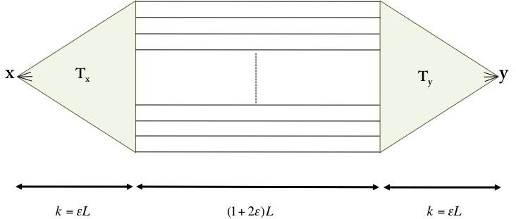
Figure 1: We create for each pair of nodes $x,y$ two node disjoint trees $T_{x},T_{y}$ of depth $k=\epsilon L$ whose leaves can be matched via a natural isomorphism and linked with edge disjoint paths of length $(1+o(1))L$ (see Section 5 for the details).

A path-based approach, Theorem 2. Before we go into mathematical details (cf. Section 5), we describe how our algorithm behind Theorem 2 works. We perform $O(n\Delta)$ queries uniformly at random to predict all possible ${n\choose 2}$ edge signs under our model, as called in Theorem 2. Let $G$ be the resulting graph. To predict the sign of the node pair $\{x,y\}$, our algorithm performs –at high level– two steps. First, we construct a subgraph $G_{x,y}(V_{x,y},E_{x,y})\subseteq G$. This subgraph is constructed using breadth first search (BFS), and consists of two isomorphic trees $T_{x},T_{y}$, each one rooted at $x,y$ respectively. The leaves of these trees can be matched and linked with edge disjoint paths; more details are given in Section 5. Pairs of nodes that map to each other under the isomorphism are written as $v,\bar{v}$, so $y$ is also $\bar{x}$. The isomorphic copies of the leaves $u\in T_{x},\bar{u}\in T_{y}$ of the two trees are connected by edge disjoint paths. This subgraph is shown in Figure 1.

Given the subgraph $G_{x,y}$, our algorithm estimates the relative coloring of pairs of nodes recursively, working from the leafs of the trees $T_{x},T_{y}$ up to the roots. That is, we first estimate $\sigma(u)\sigma(\bar{u})$ for the leaves $u,\bar{u}$ based on the path between them, and then, moving toward the roots $x$ and $y$, we estimate $\sigma(v)\sigma(\bar{v})$ based on a majority vote derived by the children. More formally, let $Z_{v,\bar{v}}$ be the estimate of $\sigma(v)\sigma(\bar{v})$ for any vertex $v$ given by the algorithm below. (Formally, this algorithm defines the random variables $Z_{u,\bar{u}}$).

• Base case: For leaf nodes $u\in T_{x}$, we define

  $$Z_{u,\bar{u}}:=\tau(P_{i})$$

  where $\tau(P_{i})$ is our estimate of $\sigma(u)\sigma(\bar{u})$ based just on observations from the path $P_{i}$ from $u\to\bar{u}$ (that is, $\tau(P_{i}):=\prod_{e\in P_{i}}\tau(e)$).

• Induction on depth: For nodes $u$ at depth $\ell$ in $T_{x}$, let $N(u)$ be children of $u$ (at depth $\ell+1$). Then, define

  $$Z_{u,\bar{u}}:=\mathrm{majority}(\{\tau(u,v)Z_{v,\bar{v}}\tau(\bar{v},\bar{u})\}_{v\in N(u)}).$$

Our induction approach collapses each path between each pair of nodes $v,\bar{v}$ (that are children of $u,\bar{u}$ respectively) at depth $\ell+1$ into a single edge, which we estimate based on our previous estimates $Z_{v,\bar{v}}$. Then, in this “collapsed” graph, we take the $\mathrm{majority}$ vote over all (disjoint) paths $u\to\bar{u}$. At the end, we output $Z_{x,y}:=Z_{x,\bar{x}}$. Using Fourier analytic techniques [31] we prove in Section 5 that

$$\Pr[Z_{x,y}=\sigma(x)\sigma(y)]\geq 1-1/n^{3}.$$

A union bound over all ${n\choose 2}$ pairs yields Theorem 2. Observe that algorithmically we do not need to perform all ${n\choose 2}$ queries to recover the two clusters, but any set of $n-1$ queries that form a spanning tree between the $n$ nodes.

A machine learning formulation. Our algorithm is heavily based on paths to predict the sign of $\{x,y\}$. Inspired by this result, we use paths as an informative feature in the context of predicting positive and negative links in online social networks. Specifically, we enrich the machine learning formulation proposed by Leskovec et al. [22] by adding four new global features as follows: for each edge $(u,v)$, we find a number of edge-disjoint paths of length three that connect $u,v$, and similarly we find edge-disjoint paths of length four. We calculate the product of the weights of each path and tally the number of positive and negative products for each path length. We add these four counts as four new dimensions. (We also tried paths of length five, but they are not as informative and are also more computationally expensive, so we do not study such paths henceforth.) We ignore directions of edges both for computational efficiency, and in order to avoid introducing too many features, as for a path of length $\ell$ there are $2^{\ell}$ possible directed versions of the path. We describe some key elements of the framework in [22] for completeness. Notice that the feature engineering is performed on the whole graph.

• Features: In addition to our four new global features, we use 23 local features to predict the sign of the edge $u\rightarrow v$: $d^{+}_{out}(u),d^{-}_{out}(u)$, $d^{+}_{in}(v),d^{-}_{in}(v),d_{out}(u),d_{in}(v)$, $C(u,v)$ where $C(u,v)$ is the embeddedness, i.e., the number common neighbors of $u,v$ (in an undirected sense), and a 16-dimensional count vector, with one coordinate for each possible configuration of a triad.

• We train a logistic regression classifier that learns a model of the form ${\bf{Pr}}\left[{+|x}\right]=\frac{1}{1+e^{-b_{0}+\sum b_{i}x_{i}}}$. Here $x=(x_{1},\ldots,x_{27})$ is our 27-dimensional feature vector.

• We create balanced datasets so that random guessing results in 50% accuracy. We perform 10-fold cross validation, i.e., we create 10 disjoint folds, each consisting of 10% of the total number of edges. For each fold, we use the remaining 90% of the edges as the training dataset for the logistic regression. We report average accuracies over these 10 folds.

4 Experimental Results

4.1 Experimental Setup

Experimental setting. Since finding the maximum number of edge-disjoint paths of short length is NP-hard [21], we implement a fast greedy heuristic: to find edge-disjoint paths of length $k$ ($k=3,4$ in our experiments) between $s,t$, we discard edge directionality, and we start BFS from $s$. As soon as we find a path of length $k$ to $t$, we check if its edges have been removed from the graph using a hash table; if not, we add the path to our collection, we remove its edges from the graph, we add them to the hash table, and we continue. At termination, we count how many positive and negative paths exist in our collection. To train a classifier, we use logistic regression. For this purpose we use Scikit-learn [32].

Datasets. Table 2 shows various publicly available online social networks (OSN) we use in our experiments together with the number of nodes $n$ and the number of edges $m$. We present in detail our findings for the first two datasets described in the following. The results for the other graphs are very similar.

Slashdot is a news website. Nodes correspond to users, and edges to their interactions. A positive sign means that a user likes another user’s comments.

Wikipedia is a free online encyclopedia, created and edited by volunteers around the world. Nodes correspond to editors, and a signed link indicates a positive or negative vote by one user on the promotion of another.

Machine specs. All experiments run on a laptop with 1.7 GHz Intel Core i7 processor and 8GB of main memory.

Code. Our code was written in Python. A demo of our code is available as a Python notebook online at github/Prediction.ipynb.

Name	$n$	$m$	Description
Slashdot (Feb. 21)	82 144	549 202	OSN [1]
Wikipedia	7 118	103 747	OSN [1]
Epinions	119 217	841 200	OSN [1]
Slashdot (Nov. 6)	77 350	516 575	OSN [1]
Slashdot (Feb. 16)	81 867	545 671	OSN [1]
Highlands tribes	16	58	SN [33]

Table 2: Datasets used in our experiments.

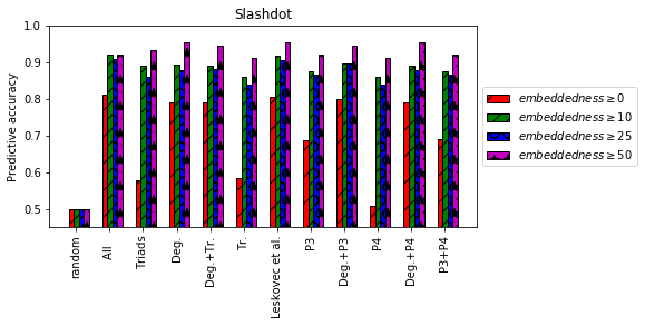
(a)

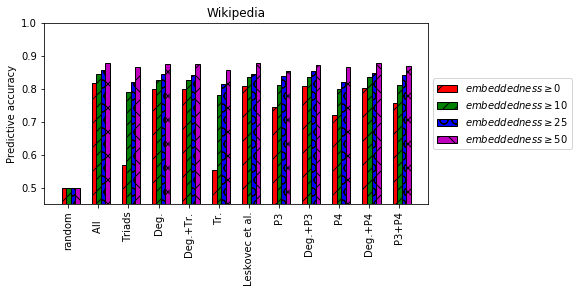
(b)

Figure 2: Average accuracy of predicting edge signs using 10-fold cross validation. (a) Slashdot, (b) Wikipedia.

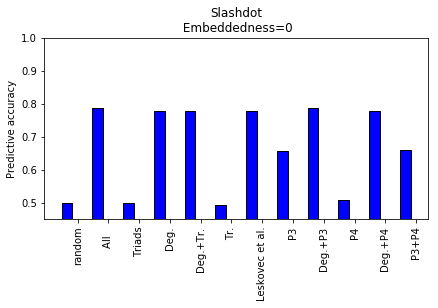
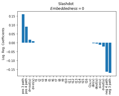
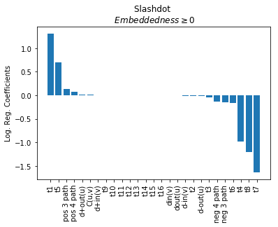
(a)	(b)	(c)
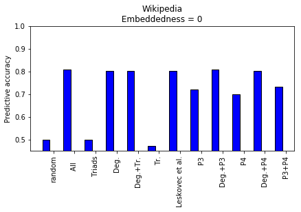
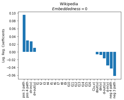
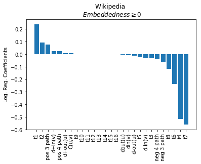
(d)	(e)	(f)

Figure 3: (a),(d) Average accuracy of predicting signs of edges with zero embeddedness using 10-fold cross validation, (b),(e) and the resulting logistic regression coefficients, for Slashdot and Wikipedia respectively. (c), (f) Learned logistic regression coefficients for the whole Slashdot and Wikipedia datasets respectively.

4.2 Empirical findings

We experiment with various combinations of the 27 features that we described in Section  3. All refers to using all 27 features, Triads to the 16-dimensional vector of triad counts, Deg to degree features, Tr. (short for triangles) to the number of common neighbors, Leskovec et al. to the 23 features used in [22], and P3, P4 to the number of negative and positive edge-disjoint paths of length 3, 4 respectively. A combination of the form P3+P4 means using the union of these features, for example counts of positive and negative edge disjoint paths of length 3 and 4 respectively.

Figures 2(a), (b) shows the performance of our classifier using different combinations of features, broken down by a lower bound on the embeddedness. For the Slashdot dataset, we observe that when we classify all edges (embeddedness $\geq 0$) P3 performs better than Triads, i.e., 68.8% vs 57.8%. Also, the performance of a Triads-based classifier is not monotonic as a function of the embeddedness lower bound. For example, when embeddedness is at least 10 the accuracy is 88.9%, whereas when it is at least 25 it becomes 86.1%. However, in general the prediction problem becomes easier as the embeddedness increases. Also, using all features, i.e., the addition of the four new features P3, P4 to the existing Leskovec et al. results in the best possible performance. Finally, paths of length 3 are more informative than paths of length 4. This is clearly seen by the logistic regression coefficients shown in Figure 3(c). We also observe that different types of triads can have significantly different regression coefficients, and that the coefficients depend significantly on the graph, as seen in Figures 3(c) and 3(f).

Figures 3(a), (d) show the average accuracy of predicting edge signs for edges with embeddedness equal to zero for the Slashdot and Wikipedia datasets respectively. When we use Triads the predictive accuracy is as only about as good as random guessing, i.e., 50%. P3 results in 65.74%, and 71.96% accuracy, P4 in 50.78%, and 69.90% accuracy for Slashdot and Wikipedia respectively. We observe that using all features leads to the best possible performances of 78.63%, and 80.92% accuracy respectively for the two datasets. The importance of paths of length 3, and 4 for edges with zero embeddedness is seen by the logistic regression coefficients in Figures 3(b), (e).

5 Algorithmic Analysis

We use the following notation. Let $\epsilon:=\frac{1}{\sqrt{\lg\lg n}}$, and

$$\Delta=O\big{(}\mathrm{max}\{\frac{1}{\delta^{4}}\log n,(\frac{1}{\delta})^{4+\frac{2+2\epsilon}{\epsilon}}\}\big{)}$$

be the average degree. We perform in total $\frac{12n\log{n}}{\delta^{4}}$ queries, and for simplicity, let the bias $0<\delta<\frac{1}{2}$ be a constant, independent of $n$. Hence, asymptotically $\Delta=\frac{12}{\delta^{4}}\log n$. Finally, let $L=\frac{\log n}{\log\Delta}$ be the diameter of the resulting random graph we obtain whp [4].

Algorithm 2 Almost-Edge-Disjoint-Paths($u,v$)

0:  $G(V,E)$, $u,v\in V(G)$

  $\epsilon\leftarrow\frac{1}{\sqrt{\log\log{n}}}$

  Using Breadth First Search (BFS) grow a tree $T_{u}$ starting from $u$ as follows.

  We use a branching factor equal to $\frac{4\log{n}}{\delta^{4}}$ until it reaches depth equal to $\epsilon L$. Similarly, grow a tree $T_{v}$ rooted at $v$, node disjoint from $T_{u}$ of equal depth.

  From each leaf $u_{i}$ ($v_{i}$) of $T_{u}$ ($T_{v}$) for $i=1,\ldots,N$ grow node disjoint trees until they reach depth $(\frac{1}{2}+\epsilon)L$ with branching factor $\frac{4\log{n}}{\delta^{4}}$. Finally, find an edge between $T_{u_{i}},T_{v_{i}}$

5.1 Subgraph construction

The next lemma follows from standard Chernoff bounds (and a union bound over vertices).

Lemma 2.

Let $G\sim G(n,\frac{12\log{n}}{\delta^{4}n})$ be a random binomial graph. Then whp all vertices have degree greater than $\frac{5\log{n}}{\delta^{4}}$.

Now we proceed to our construction of sufficiently enough almost edge-disjoint paths. Our construction is based on standard techniques in random graph theory [6, 14, 16, 37], we include the full proofs for completeness.

Lemma 3.

Let $G\sim G(n,p)$ where $p=\frac{12\log n}{\delta^{4}n}:=\frac{c_{\delta}\log n}{n}$. Fix $t\in\mathbb{Z}^{+}$ and $0<\alpha<1$. Then, whp there does not exist a subset $S\subseteq[n]$, such that $|S|\leq\alpha tL$ and $e[S]\geq|S|+t$.

Proof.

Set $s=|S|$.Then,

$${\bf{Pr}}\left[{\exists S:s\leq\alpha tL\text{~{}~{}and~{}~{}}e[S]\geq s+t}\right] \leq\sum_{s\leq\alpha tL}\binom{n}{s}\binom{\binom{s}{2}}{s+t}p^{s+t}\leq$$

$$\sum_{s\leq\alpha tL}\left(\frac{ne}{s}\right)^{s}\left(\frac{es^{2}p}{2(s+t)}\right)^{s+t} \leq\sum_{s\leq\alpha tL}(e^{2+o(1)}\log{n})^{s}\left(\frac{\tfrac{c_{\delta}}{2}es\log{n}}{n}\right)^{t}\leq$$

$$\alpha tL\left((e^{2+o(1)}\log{n})^{\alpha L}\left(\frac{\tfrac{c_{\delta}}{2}e\alpha t\log^{2}{n}}{n\log{\log{n}}}\right)\right)^{t} <\frac{1}{n^{(1-\alpha-o(1))t}}.$$

∎

Lemma 4.

Let $T$ be a rooted (subgraph) tree of depth at most $\frac{4L}{7}$ and let $v$ be a vertex not in $T$. Then with probability $1-o(n^{-3})$, $v$ has at most $10$ neighbors in $T$, i.e., $|N(v)\cap T|\leq 10$.

Proof.

Let $T$ be a rooted tree of depth at most $\frac{4L}{7}$ and let $S$ consist of $v$, the neighbors of $v$ in $T$ plus the ancestors of these neighbors. Set $b=|N(v)\cap T|$. Then $|S|\leq 4bL/7+1\leq 3bL/5$ and $e[S]=|S|+b-2$. It follows from Lemma 3 with $\alpha=3/5$ and $t=8$, that we must have $b\leq 10$ with probability $1-o(n^{-3})$. ∎

We show that by growing trees iteratively we can construct sufficiently many edge-disjoint paths for $n$ sufficiently large.

Lemma 5.

Let $k=\epsilon L$. For all pairs of vertices $x,y\in[n]$ there exists a subgraph $G_{x,y}(V_{x,y},E_{x,y})$ of $G$ as shown in Figure 1, whp. The subgraph consists of two isomorphic vertex disjoint trees $T_{x},T_{y}$ rooted at $x,y$ each of depth $k$. $T_{x}$ and $T_{y}$ both have a branching factor of $\frac{4\log n}{\delta^{4}}$. If the leaves of $T_{x}$ are $x_{1},x_{2},\ldots,x_{\tau},\tau\geq n^{4\epsilon/5}$ then $y_{i}=f(x_{i})$ where $f$ is a natural isomorphism. Between each pair of leaves $(x_{i},y_{i}),i=1,2,\ldots,m$ there is a path $P_{i}$ of length $(1+2\epsilon)L$. The paths $P_{i},i=1,2,\ldots,\tau,\ldots$ are edge disjoint.

Proof.

Since we have to do this for all pairs $x,y$, we note without further comment that likely (resp. unlikely) events will be shown to occur with probability $1-o(n^{-2})$ (resp. $o(n^{-2}$)).

To find the subgraph shown in Figure 1 we grow tree structures as shown in Figure 4. Specifically, we first grow a tree from $x$ using BFS until it reaches depth $k$. Then, we grow a tree starting from $y$ again using BFS until it reaches depth $k$. Finally, once trees $T_{x},T_{y}$ have been constructed, we grow trees from the leaves of $T_{x}$ and $T_{y}$ using BFS for depth $\gamma=(\frac{1}{2}+\epsilon)L$. We analyze these processes, explaining in detail for $T_{x}$ and outlining the differences for the other trees. We use the notation $D_{i}^{(\rho)}$ for the number of vertices at depth $i$ of the BFS tree rooted at $\rho$.

First we grow $T_{x}$. As we grow the tree via BFS from a vertex $v$ at depth $i$ to vertices at depth $i+1$ certain bad edges from $v$ may point to vertices already in $T_{x}$. Lemma 4 shows with probability $1-o(n^{-3})$ there can be at most 10 bad edges emanating from $v$.

Hence, we obtain the recursion

$$D_{i+1}^{(x)}\geq\left(\frac{5\log{n}}{\delta^{4}}-10\right)(D_{i}^{(x)}-1)\geq\frac{4\log{n}}{\delta^{4}}D_{i}^{(x)}.$$ (1)

Therefore the number of leaves satisfies

$$D_{k}^{(x)}\geq\Big{(}\frac{4\log n}{\delta^{4}}\Big{)}^{\epsilon L}\geq n^{4\epsilon/5}.$$ (2)

We can make the branching factors exactly $\frac{4\log n}{\delta^{4}}$ by pruning. We do this so that the trees $T_{x},T_{y}$ are isomorphic to each other. With a similar argument $D_{k}^{(y)}\geq n^{\frac{4}{5}\epsilon}$. Specifically, the only difference is that now we also say an edge is bad if the other endpoint is in $T_{x}$. This immediately gives

$$D_{i+1}^{(y)}\geq\left(\frac{5\log{n}}{\delta^{4}}-20\right)(D_{i}^{(y)}-1)\geq\frac{4\log{n}}{\delta^{4}}D_{i}^{(y)}$$

and the required conclusion.

Similarly, from each leaf $x_{i}\in T_{x}$ and $y_{i}\in T_{y}$ we grow trees $\widehat{T}_{x_{i}},\widehat{T}_{y_{i}}$ of depth $\gamma=\big{(}\frac{1}{2}+\epsilon\big{)}L$ using the same procedure and arguments as above. Lemma 4 implies that there are at most 20 edges from the vertex $v$ being explored to vertices in any of the trees already constructed (at most 10 to $T_{x}$ plus any trees rooted at an $x_{i}$ and another 10 for $y$). The number of leaves of each $\widehat{T}_{x_{i}}$ now satisfies

$$\widehat{D}_{\gamma}^{(x_{i})}\geq(\frac{4}{\delta^{4}}\log{n})^{\gamma+1}\geq n^{\frac{1}{2}+\frac{4}{5}\epsilon}.$$

The result is similar for $\widehat{D}_{\gamma}^{(y_{i})}$.

Observe next that BFS does not condition on the edges between the leaves $X_{i},Y_{i}$ of the trees $\widehat{T}_{x_{i}}$ and $\widehat{T}_{y_{i}}$. That is, we do not need to look at these edges in order to carry out our construction. On the other hand we have conditioned on the occurrence of certain events to imply a certain growth rate. We handle this technicality as follows. We go through the above construction and halt if ever we find that we cannot expand by the required amount. Let ${\bf A}$ be the event that we do not halt the construction i.e. we fail the conditions of Lemmas 3 or 4. We have ${\bf{Pr}}\left[{{\bf A}}\right]=1-o(1)$ and so,

$${\bf{Pr}}\left[{\exists i:e(X_{i},Y_{i})=0\mid{\bf A}}\right] \leq\frac{{\bf{Pr}}\left[{\exists i:e(X_{i},Y_{i})=0}\right]}{\Pr({\bf A})}$$

$$\leq 2n^{\frac{4\epsilon}{5}}(1-p)^{n^{1+\frac{8\epsilon}{5}}} \leq n^{-n^{\epsilon}}.$$

We conclude that whp there is always an edge between each $X_{i},Y_{i}$ and thus a path of length at most $(1+2\epsilon)L$ between each $x_{i},y_{i}$. ∎

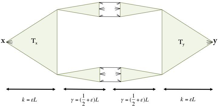
Figure 4: We create edge disjoint paths for each isomorphic pair of leaves $u,\bar{u}$ in the two node disjoint trees $T_{x},T_{y}$ (see Lemma 5 for the details).

Using elementary data structures, our algorithm runs in total expected run time $O(n^{2}(n+m))=O(\frac{n^{3}\log{n}}{\delta^{4}})$.

5.2 Algorithm Correctness

Recall from Section 3 that $Z_{u,\bar{u}}:=\mathrm{maj}(\{\tau(u,v)Z_{v,\bar{v}}\tau(\bar{v},\bar{u})\}_{v\in N(u)})$. Therefore, note that at any level $k$ in the tree, the random variables $\{Z_{u,\bar{u}}\}$ are independent for all nodes $u$ at level $k$. (This is true in the base case by path-disjointedness, and preserved by the induction). The key Lemma 6 follows. In simple terms, it shows that the bias of our estimator improves by roughly a $\delta^{2}\sqrt{\Delta}$ factor at each level.

Lemma 6.

Suppose that for all $v\in T_{x}$ at depth $k+1$, we have

$$\Pr[Z_{v,\bar{v}}=\sigma(v)\sigma(\bar{v})]\geq 1/2+\gamma$$

Then, for all $u\in T_{x}$ at depth $k$, we have

$$\Pr[Z_{u,\bar{u}}=\sigma(u)\sigma(\bar{u})]\geq 1/2+\min(\gamma(c_{1}\delta^{2}\sqrt{\Delta}),c_{2})$$

for some universal $c_{1},c_{2}$.

The proof invokes the Majority Bias Lemma (see Lemma 8) that we prove at the end of this section.

Proof.

It is more convenient to work with the bias

$${\mathbb{E}}\left[{Z_{v,\bar{v}}\sigma(v)\sigma(\bar{v})}\right]=2{\bf{Pr}}\left[{Z_{v,\bar{v}}=\sigma(v)\sigma(\bar{v})}\right]-1\geq 2\gamma$$

By the recursive definition,

$$Z_{u,\bar{u}}:=\mathrm{maj}(\{\tau(u,v)Z_{v,\bar{v}}\tau(\bar{v},\bar{u})\}_{v\in N(u)})$$

So:

$${\mathbb{E}}\left[{Z_{u,\bar{u}}\sigma(u)\sigma(\bar{u})}\right] =$$

$${\mathbb{E}}\left[{\mathrm{maj}(\{\tau(u,v)Z_{v,\bar{v}}\tau(\bar{v},\bar{u})\}_{v\in N(u)})\sigma(u)\sigma(\bar{u}))}\right] =$$

$${\mathbb{E}}\left[{\mathrm{maj}(\{\sigma(u)\tau(u,v)Z_{v,\bar{v}}\tau(\bar{v},\bar{u})\sigma(\bar{u})\}_{v\in N(u)})}\right] =$$

$$\mathbb{E}[\mathrm{maj}(\{\sigma(u)\sigma(v)\tau(u,v)\cdot\sigma(v)Z_{v,\bar{v}}\sigma(\bar{v})\cdot \sigma(\bar{v})\sigma(\bar{u})\tau(\bar{v},\bar{u})\}_{v\in N(u)})]=$$

$$\mathbb{E}[\mathrm{maj}(\{\eta_{u,v}\cdot\sigma(v)Z_{v,\bar{v}}\sigma(\bar{v})\cdot\eta_{\bar{u},\bar{v}}\}_{v\in N(u)})]$$

For any single $v\in N(u)$ we have $\mathbb{E}[\eta_{u,v}]\mathbb{E}[\sigma(v)Z_{v,\bar{v}}\sigma(\bar{v})]\mathbb{E}[\eta_{\bar{u},\bar{v}}]\geq\delta^{2}2\gamma$. Then by Lemma 8, taking $\mathrm{majority}$ over $\Delta$ such coins amplifies the bias to $\min(c_{1}\gamma\delta^{2}\sqrt{\Delta},c_{2})$, as desired. ∎

To conclude the analysis, we show in Lemma 7 that doing $\epsilon L$ levels of this amplifies the bias to a constant. Then we are done, because the root will take the majority of $\Delta=\Omega(\log(n)/\delta^{4})$ independent coins, each with bias $O(\delta^{2})$, and so the estimate is correct with high probability. The following amplification result holds:

Lemma 7.

For nodes $u\in T_{x}$ that are $\epsilon L$ levels up from the leaves, we have that

$$\Pr[Z_{v,\bar{v}}=\sigma(v)\sigma(\bar{v})]\geq 1/2+c_{2}$$

Proof.

Note that at a leaf $u\in T_{x}$, the bias is

$$\mathbb{E}[Z_{u,\bar{u}}\sigma(u)\sigma(\bar{u})]=\mathbb{E}[\tau(P_{i})\sigma(u)\sigma(\bar{u})]=\mathbb{E}[\prod_{e\in P_{i}}\eta_{e}]\geq\delta^{(1+2\epsilon)L}$$

where $P_{i}$ is the path from $u\to\bar{u}$, of length at most $(1+2\epsilon)L$.

Then we apply the amplification lemma inductively for $\epsilon L$ levels, starting with this bias at the leaves. It suffices to show that

$$(c_{1}\delta^{2}\sqrt{\Delta})^{\epsilon L}\exp\left(-L(1+2\epsilon)\log\frac{1}{\delta}\right)>1$$

This means that $\log(c_{1}\delta^{2}\sqrt{\Delta})>\frac{1}{\epsilon}(1+2\epsilon)\log\left(\frac{1}{\delta}\right)$. Equivalently, solving for $\Delta$

$$\Delta>\left(\frac{1}{\delta}\right)^{4}\left(\frac{1}{\delta}\right)^{\frac{2+2\epsilon}{\epsilon}},$$

which holds for our choice of $\Delta$ as long as $\delta$ is a constant. ∎

Lemma 8 (Majority Bias Lemma).

Let $X_{1},X_{2},\ldots X_{n}$ be independent random variables with $X_{i}\in\{\pm 1\}$ and $\mathbb{E}X_{i}\geq\delta$. Then $\mathbb{E}\mathrm{maj}(X_{1},\ldots X_{n})\geq\min(c_{1}\sqrt{n}\delta,c_{2})$ for some universal constants $c_{1}$ and $c_{2}$.

Proof.

First we prove the case when $\mathbb{E}X_{i}=\delta$ for all $i$. Consider the Fourier transform of $\mathrm{maj}(X_{1},\ldots,X_{n})=\sum_{S\subset[n]}\widehat{\mathrm{maj}_{n}}(S)\chi_{S}$, where $\chi_{S}=\prod_{i\in S}X_{i}$ and $\widehat{\mathrm{maj}_{n}}(S)\chi_{S}$ are the corresponding Fourier coefficients. Specifically, for even $|S|$, $\widehat{\mathrm{maj}_{n}}(S)=0$, and for odd $|S|$,

$$\widehat{\mathrm{maj}_{n}}(S)=(-1)^{\tfrac{k-1}{2}}\frac{{\frac{n-1}{2}\choose\frac{k-1}{2}}}{{n-1\choose k-1}}\frac{2}{2^{n}}{n-1\choose\frac{n-1}{2}}.$$

Then

$$\mathbb{E}[\mathrm{maj}(X_{1},\ldots X_{n})] =\sum_{S}\widehat{\mathrm{maj}_{n}}(S)\mathbb{E}[\chi_{S}]$$

$$=\sum_{S}\widehat{\mathrm{maj}_{n}}(S)\delta^{|S|}$$

$$\geq\sum_{|S|=1}\widehat{\mathrm{maj}_{n}}(S)\delta-\left|\sum_{|S|\geq 2}\widehat{\mathrm{maj}_{n}}(S)\delta^{|S|}\right|$$

$$\geq\sum_{|S|=1}\widehat{\mathrm{maj}_{n}}(S)\delta-\sum_{k\geq 2}\delta^{k}\left(\sum_{|S|=k}|\widehat{\mathrm{maj}_{n}}(S)|\right).$$

And we have for $|S|=1$

$$\sum_{|S|=1}\widehat{\mathrm{maj}_{n}}(S)=\frac{2}{2^{n}}{n-1\choose\frac{n-1}{2}}=\frac{2\sqrt{2}}{\sqrt{\pi}}\sqrt{n}$$

For $|S|=k\geq 2$ using the Cauchy-Schwarz inequality we can provide an upper bound

$$\sum_{|S|=k}|\widehat{\mathrm{maj}_{n}}(S)|\leq\sqrt{{n\choose k}}\sqrt{\sum_{|S|=k}\widehat{\mathrm{maj}_{n}}(S)^{2}},$$

and Parseval’s identity implies $\sum_{|S|=k}\widehat{\mathrm{maj}_{n}}(S)^{2}\leq\sum_{S\subset[n]}\widehat{\mathrm{maj}_{n}}(S)^{2}=1$, which ultimately gives an upper bound $\sum_{|S|=k}|\widehat{\mathrm{maj}_{n}}(S)|\leq n^{k/2}$.

Plugging those two together, when $\delta\sqrt{n}\leq\frac{1}{2}$, we have

$$\mathbb{E}[\mathrm{maj}(X_{1},\ldots X_{n})]\geq\frac{2\sqrt{2}}{\sqrt{\pi}}\sqrt{n}\delta-\sum_{k\geq 2}(\sqrt{n}\delta)^{k}=\Omega(\sqrt{n}\delta).$$

When $\delta\sqrt{n}>\frac{1}{2}$, by Chernoff bound

$$\mathbb{E}[\mathrm{maj}(X_{1},\ldots X_{n})]=\Pr[\sum_{i}X_{i}>0]\geq 1-e^{-\Omega(\delta^{2}n)}=\Omega(1)$$

This gives $\mathbb{E}[\mathrm{maj}(X_{1},\ldots X_{n})]\geq\min(c_{1}\sqrt{n}\delta,c_{2})$ for $\mathbb{E}[X_{i}]=\delta$. The general case when $\mathbb{E}[X_{i}]\geq\delta$ follows readily from the monotonicity of the majority function.

∎

6 Conclusion

An interesting open problem concerns the extension of our results to $k$ clusters. Specifically, our clustering model naturally extends to the case where there are more than two clusters [27]. In this case the set $V$ of $n$ items belong to $k$ clusters. When we query the pair of nodes $\{u,v\}$ we obtain a noisy answer on whether $u,v$ belong to the same cluster or not. Can we design a polynomial time algorithm that performs $O(\frac{kn\log n}{\delta^{2}})$ queries for all $0<\delta<1$? From an experimental point of view, we plan to experiment with other types of classifiers in addition to logistic regression classifiers to diagnose whether an additional improvement in classification accuracy can be achieved.

References

- [1] Stanford network analysis project, July 2017. http://snap.stanford.edu/data/index.html.
- [2] E. Abbe, A. S. Bandeira, and G. Hall. Exact recovery in the stochastic block model. IEEE Transactions on Information Theory, 62(1):471–487, 2016.
- [3] N. Bansal, A. Blum, and S. Chawla. Correlation clustering. Machine Learning, 56(1-3):89–113, 2004.
- [4] B. Bollobás. Random graphs. In Modern Graph Theory. Springer, 1998.
- [5] F. Bonchi, D. Garcia-Soriano, and E. Liberty. Correlation clustering: from theory to practice. In KDD, page 1972, 2014.
- [6] A. Z. Broder, A. M. Frieze, S. Suen, and E. Upfal. Optimal construction of edge-disjoint paths in random graphs. SIAM Journal on Computing, 28(2):541–573, 1998.
- [7] E. J. Candès, J. Romberg, and T. Tao. Robust uncertainty principles: Exact signal reconstruction from highly incomplete frequency information. IEEE Transactions on information theory, 52(2):489–509, 2006.
- [8] D. Cartwright and F. Harary. Structural balance: a generalization of heider’s theory. Psychological review, 63(5):277, 1956.
- [9] N. Cesa-Bianchi, C. Gentile, F. Vitale, G. Zappella, et al. A correlation clustering approach to link classification in signed networks. In COLT, pages 34–1, 2012.
- [10] Y. Chen, A. Jalali, S. Sanghavi, and H. Xu. Clustering partially observed graphs via convex optimization. Journal of Machine Learning Research, 15(1):2213–2238, 2014.
- [11] Y. Chen, S. Sanghavi, and H. Xu. Clustering sparse graphs. In Advances in neural information processing systems, pages 2204–2212, 2012.
- [12] K.-Y. Chiang, C.-J. Hsieh, N. Natarajan, I. S. Dhillon, and A. Tewari. Prediction and clustering in signed networks: a local to global perspective. Journal of Machine Learning Research, 15(1):1177–1213, 2014.
- [13] K.-Y. Chiang, N. Natarajan, A. Tewari, and I. S. Dhillon. Exploiting longer cycles for link prediction in signed networks. In Proceedings of the 20th ACM international conference on Information and knowledge management, pages 1157–1162. ACM, 2011.
- [14] A. Dudek, A. M. Frieze, and C. E. Tsourakakis. Rainbow connection of random regular graphs. SIAM Journal on Discrete Mathematics, 29(4):2255–2266, 2015.
- [15] D. Easley and J. Kleinberg. Networks, crowds, and markets: Reasoning about a highly connected world. Cambridge University Press, 2010.
- [16] A. Frieze and C. E. Tsourakakis. Rainbow connectivity of sparse random graphs. In Approximation, Randomization, and Combinatorial Optimization (APPROX-RANDOM), pages 541–552. Springer, 2012.
- [17] B. Hajek, Y. Wu, and J. Xu. Achieving exact cluster recovery threshold via semidefinite programming. IEEE Transactions on Information Theory, 62(5):2788–2797, 2016.
- [18] F. Harary. On the notion of balance of a signed graph. The Michigan Mathematical Journal, 2(2):143–146, 1953.
- [19] F. Heider. Attitudes and cognitive organization. The Journal of psychology, 21(1):107–112, 1946.
- [20] J. P. Hou, A. Emad, G. J. Puleo, J. Ma, and O. Milenkovic. A new correlation clustering method for cancer mutation analysis. arXiv preprint arXiv:1601.06476, 2016.
- [21] A. Itai, Y. Perl, and Y. Shiloach. The complexity of finding maximum disjoint paths with length constraints. Networks, 12(3):277–286, 1982.
- [22] J. Leskovec, D. Huttenlocher, and J. Kleinberg. Predicting positive and negative links in online social networks. In Proceedings of the 19th international conference on World Wide Web (WWW), pages 641–650. ACM, 2010.
- [23] J. Leskovec, D. Huttenlocher, and J. Kleinberg. Signed networks in social media. In Proceedings of the SIGCHI conference on Human Factors in Computing Systems, pages 1361–1370. ACM, 2010.
- [24] K. Makarychev, Y. Makarychev, and A. Vijayaraghavan. Correlation clustering with noisy partial information. In Proceedings of the Conference on Learning Theory (COLT), volume 6, page 12, 2015.
- [25] C. Mathieu and W. Schudy. Correlation clustering with noisy input. In Proceedings of the twenty-first annual ACM-SIAM symposium on Discrete Algorithms, pages 712–728. Society for Industrial and Applied Mathematics, 2010.
- [26] A. Mazumdar and B. Saha. Clustering via crowdsourcing. arXiv preprint arXiv:1604.01839, 2016.
- [27] A. Mazumdar and B. Saha. Clustering with noisy queries. In Advances in Neural Information Processing Systems, pages 5790–5801, 2017.
- [28] F. McSherry. Spectral partitioning of random graphs. In Proceedings. 42nd IEEE Symposium on Foundations of Computer Science (FOCS), pages 529–537. IEEE, 2001.
- [29] M. Mitzenmacher and C. E. Tsourakakis. Predicting signed edges with queries. arXiv preprint arXiv:1609.00750, 2016.
- [30] M. Mitzenmacher and E. Upfal. Probability and computing: Randomized algorithms and probabilistic analysis. Cambridge university press, 2005.
- [31] R. O’Donnell. Analysis of boolean functions. Cambridge University Press, 2014.
- [32] F. Pedregosa, G. Varoquaux, A. Gramfort, V. Michel, B. Thirion, O. Grisel, M. Blondel, P. Prettenhofer, R. Weiss, V. Dubourg, et al. Scikit-learn: Machine learning in python. Journal of Machine Learning Research, 12(Oct):2825–2830, 2011.
- [33] K. E. Read. Cultures of the Central Highlands, New Guinea. Southwestern J. of Anthropology, 10(1):1–43, 1954.
- [34] B. Settles. Active learning literature survey. University of Wisconsin, Madison, 52(55-66):11, 2010.
- [35] R. Shamir, R. Sharan, and D. Tsur. Cluster graph modification problems. Discrete Applied Mathematics, 144(1):173–182, 2004.
- [36] S. Strogatz. The enemy of my enemy, February 2014. https://opinionator.blogs.nytimes.com/2010/02/14/the-enemy-of-my-enemy/.
- [37] C. E. Tsourakakis. Mathematical and Algorithmic Analysis of Network and Biological Data. PhD thesis, Carnegie Mellon University, 2013.
- [38] V. Verroios and H. Garcia-Molina. Entity resolution with crowd errors. In IEEE 31st International Conference on Data Engineering (ICDE), pages 219–230. IEEE, 2015.
- [39] V. Vu. A simple svd algorithm for finding hidden partitions. arXiv preprint arXiv:1404.3918, 2014.