Influence of Clustering on Cascading Failures in Interdependent Systems

Abstract

We study the influence of clustering, more specifically triangles, on cascading failures in interdependent networks or systems, in which we model the dependence between comprising systems using a dependence graph. First, we propose a new model that captures how the presence of triangles in the dependence graph alters the manner in which failures transmit from affected systems to others. Unlike existing models, the new model allows us to approximate the failure propagation dynamics using a multi-type branching process, even with triangles. Second, making use of the model, we provide a simple condition that indicates how increasing clustering will affect the likelihood that a random failure triggers a cascade of failures, which we call the probability of cascading failures (PoCF). In particular, our condition reveals an intriguing observation that the influence of clustering on PoCF depends on the vulnerability of comprising systems to an increasing number of failed neighboring systems and the current PoCF, starting with different types of failed systems. Our numerical studies hint that increasing clustering impedes cascading failures under both (truncated) power law and Poisson degree distributions. Furthermore, our finding suggests that, as the degree distribution becomes more concentrated around the mean degree with smaller variance, increasing clustering will have greater impact on the PoCF. A numerical investigation of networks with Poisson and power law degree distributions reflects this finding and demonstrates that increasing clustering reduces the PoCF much faster under Poisson degree distributions in comparison to power law degree distributions.

1 Introduction

Many modern systems that provide critical services we rely on consist of interdependent systems. Examples include modern information and communication networks/systems, power systems, manufacturing systems, and transportation systems, among others. In order to deliver their services, the comprising or component systems (CSes) must work together and oftentimes support each other.

Growing interdependence among CSes also exposes a source of vulnerability: the failure of one CS can spread to other CSes via dependence because a CS may no longer be able to function without the support from failed CS(es). From this viewpoint, it is obvious that the overall robustness of the system to failures will depend on the underlying dependence structure among CSes. We adopt a dependence graph to capture such interdependence among CSes, which we assume is neutral, i.e., there are no degree correlations between neighbors.

Despite a growing interest in modeling and understanding the robustness of large, complex systems (e.g., [1, 2, 7, 26, 38, 41, 42, 43, 47]), intricate interdependence among CSes makes their analysis challenging. Furthermore, to the best of our knowledge, there is no extensive theory or design guidelines that allow us to answer even seemingly basic questions.

Many of earlier studies that investigated the cascading behavior of failures in interdependent networks or systems, including our own, assumed tree-like propagation of failures (e.g., [27, 28, 29, 44, 46]). But, it is well documented that many real networks exhibit much higher clustering, more formally known as transitivity, than classical random graphs (e.g., Erd$\ddot{\rm o}$s-R$\acute{\rm e}$nyi random graphs or configuration models [5, 34]). Although how clustering is introduced in different real networks is still an open question, this observation led to new models that can generate clustered random graphs, e.g., [23, 32, 36].

Of particular concern is a widespread outbreak of failures among CSes, which can compromise the function of the overall system, thereby risking a potentially catastrophic system-level failure. We refer to a cascade of failures or cascading failures as an event in which the system experiences widespread failures well beyond the local neighborhood around the initial failure and, in the absence of remedial actions, the spread of failures slows down only when newly failed CSes no longer have other CSes they can cause to fail. A key question we are interested in is: how does clustering observed in real networks change the likelihood that a random failure of a CS leads to a cascade of failures in a large system?

The goal of our study is two-fold: (i) to propose a new model that will allow researchers to borrow existing tools in order to study the effects of clustering or transitivity, and (ii) to complement existing studies (summarized in Section 2) and contribute to the emerging theory on complex systems, by examining the impact of clustering on the robustness of the systems with respect to random failures of CSes. Our hope is that the new findings and insight reported here will help engineers and researchers better understand the influence of critical system properties, including clustering, and incorporate them into design guidelines of complex systems.

In order to answer the aforementioned question of interest to us, we develop a new model for capturing the influence of clustering on the likelihood of a random failure triggering cascading failures in large systems comprising many CSes. More precisely, it models the effect of triangles in a dependence graph on transmission of failures from affected CSes to their neighbors, as did the authors of [19, 32], but in a very different fashion.

Our model differs from existing models employed to study similar effects: they account for the influence of triangles (or other short cycles) either by modifying degree distributions to model the joint distributions of independent edge degrees and triangle degrees [19, 32, 47] or by replicating nodes to create cliques of size equal to their degrees [15, 16]. Instead, our model identifies the scenarios where a triangle among three CSes in the dependence graph alters the manner in which failures propagate locally. In so doing, it allows us to capture the dynamics of failure propagation with the presence of triangles.

A key benefit of our model is that it allows us to leverage an extensive set of tools available for branching processes: as pointed out in [32], it was believed that the presence of short cycles due to high clustering renders the theory of (multi-type) branching processes inapplicable. However, we will demonstrate that, by keeping track of what we call immediate parents and children, we can approximate failure propagation using a multi-type branching process. As a result, we are able to use existing tools to estimate the likelihood of experiencing cascading failures in large systems. This in turn allows us to derive a simple, yet intuitive condition (Theorem 1) that tells us how increasing clustering would change the likelihood of experiencing cascading failures.

Our findings, to some extent, corroborate earlier findings obtained using different models. Moreover, our main result (Theorem 1) reveals interesting insight that sheds new light on the complicated relation between system parameters and the influence of clustering.

Although our study is carried out in the framework of propagating failures in interdependent systems, we suspect that the basic model and approach as well as key findings are applicable to other applications with suitable changes. These applications include (i) information or rumor propagation or new technology adoption via social networks, (ii) an epidemic of disease in a society (e.g., cities or countries), and (iii) spread of malware in the Internet.

1.1 A summary of main contributions

The main contributions of our study can be summarized as follows.

F1. We propose a new model that captures the influence of triangles in dependence graphs on failure spreading dynamics. Unlike existing models (e.g., [15, 16, 32, 36]), we explicitly model the manner in which a triangle alters how failure transmits between CSes. Therefore, it enables us to study the effect of clustering in dependence graphs on failure propagation dynamics and the vulnerability of the system to cascading failures, which we measure using the probability of cascading failures (PoCF).

As mentioned earlier, the model allows us to borrow a rich set of existing tools by approximating failure propagations using a multi-type branching process [20]. Moreover, it separates the influence of clustering on PoCFs from that of degree correlations, which is a problem observed with some existing models [19, 32].

F2. Our main finding (Theorem 1) illustrates that the influence of clustering on PoCF is rather complicated in that it depends on the ratio of PoCFs and infection probabilities of different types of CSes, which will be defined precisely in Section 4. However, there exists a simple condition that tells us whether higher clustering facilitates or impedes cascading failures.

F3. Numerical studies reveal that increasing clustering tends to impede cascades of failures, rendering the system more robust to random failures. In addition, clustering has greater influence on PoCFs when the degree distribution in the dependence graph is more concentrated around the mean with smaller variance. In particular, our study indicates that the PoCF decreases more rapidly with increasing clustering under Poisson degree distributions in comparison to power law degree distributions. We offer an intuitive explanation for this observation on the basis of our model and main finding (Theorem 1).

A few words on notation: throughout the paper, we will use boldface letters or symbols to denote (row) vectors or vector functions. For instance, ${\bf d}$ denotes a vector, and the $j$-th element of ${\bf d}$ is denoted by $d_{j}$. Vector ${\bf 1}$ represents the vector of ones of an appropriate dimension. The set ${\mathbbm{Z}}_{+}$ (resp. ${\rm I\kern-1.5ptN}$) denotes the set of nonnegative integers $\{0,1,2,\ldots\}$ (resp. positive integers $\{1,2,3,\ldots\}$). Finally, all vector inequalities are assumed componentwise.

The rest of the paper is organized as follows: Section 2 summarizes existing studies that are most closely related to our study. Section 3 delineates the dependence graphs and infection graphs we use to model the propagation of failures throughout the system, followed by a more detailed description of the transmission of failures among CSes and the influence of triangles in Section 4. Section 5 outlines the multi-type branching process we employ to approximate failure propagations and PoCFs in large systems. Sections 6 and 7 present our main analytical finding and numerical studies, respectively. We provide the proof of the main finding in Section 8 and then conclude in Section 9.

2 Related Literature

There is already extensive literature on the topic of epidemics, information propagation and cascading failures (e.g., [1, 3, 4, 7, 34, 44]), which cuts across multiple disciplines (e.g., epidemiology [11, 18, 37, 39], finance [8, 9], social networks [22, 33], and technological networks [12, 13, 27]). Given the large volume of literature, it would be an unwise exercise to attempt to provide a summary of all related studies. Furthermore, although the topic of clustering has seen a renewed interest recently, especially in the context of social networks and technological networks and its role in failure spreading, it has been studied in the past in different settings, including population biology and epidemiology [17, 25]. For these reasons, here we only summarize the most relevant studies that deal with the effects of clustering on cascading behavior in networks. To improve readability, even though there are some differences in the employed models, we use the term ‘cascade’ synonymously with ‘epidemic’ and ‘contagion’ in the remainder of this section because the studied events or phenomena are similar.

As stated in Section 1, earlier (classical) random graph models proved to be unsuitable for describing many real networks; as the network sizes increase, they typically lead to tree-like structures and fail to reproduce some salient features of real networks, including the presence of short cycles which leads to higher clustering. In order to address the shortcomings of the random graph models, Miller [32] and Newman [36] independently proposed a new random graph model by extending the classical configuration model, which can produce clustered networks with tunable parameters: unlike in the classical configuration model where only a degree sequence or probability is specified, the new model specifies the joint probability $p_{st}(k_{s},k_{t})$ of two degrees – independent edge degree $k_{s}$ and triangle degree $k_{t}$; an independent edge of a node is an edge with a neighbor which is not a part of a triangle. Since a triangle has two incident edges on the node, the total degree of a node with degrees $(k_{s},k_{t})$ is $k_{s}+2\times k_{t}$.

Utilizing this new random graph model, Miller [32] investigated the impact of clustering with respect to both cascade size and threshold. His study shows that, although clustered networks could exhibit a smaller cascade threshold, compared to a configuration model with an identical degree distribution, this is caused by the degree correlations, also known as assortativity or assortative mixing, introduced in the process of generating clustered networks. When networks with similar degree correlations are compared, clustering raises the cascade threshold and diminishes the cascade size.

In another study using the same model, Hackett et. al [19] examined the influence of clustering on the expected cascade size in both site and bond percolation as well as the Watts’ random threshold model in $z$-regular graphs. They showed that clustering reduces the cascade size in the case of bond and site percolation. For the Watts’ model in the $z$-regular graphs, their finding suggests that the impact of clustering depends on the value of $z$.

In another line of interesting studies, Coupechoux and Lelarge proposed a new random graph model where some nodes are replaced by cliques of size equal to their degrees [15, 16]. Making use of this new model, they examined the influence of clustering in social networks on diffusion and contagion in (random) networks. Their key findings include the observation that, in the contagion model with symmetric thresholds, the effects of clustering on cascade threshold depend on the mean node degree; for small mean degrees, clustering impedes cascades, whereas for large mean degrees, cascades are facilitated by clustering.

Although their contagion model is similar to our model, there is a key difference; while replicating the nodes to generate cliques in the random graphs, their model assumes that the contagion thresholds of all cloned nodes in a clique are identical. In our model, however, the nodes forming triangles can have different thresholds, which we feel is more realistic in many cases. As we will show, this seemingly innocuous difference has a significant impact on the effects of clustering on cascading behavior.

In [47], Zhuang and Ya$\breve{\rm g}$an extended the model of Miller [32] and Newman [36] to study information propagation in a multiplex network with two layers representing an online social network (OSN) and a physical network, both of which have high clustering. Only a subset of vertices in the physical network are assumed to be active in the OSN. Their key findings are: (a) clustering consistently impedes cascades of information to a large number of nodes with respect to both the critical threshold of information cascade and the mean size of cascades; and (b) information transmissibility (i.e., average probability of information transmission over a link) has significant impact; when the transmissibility is low, it is easier to trigger a cascade of information propagation with a smaller, densely connected OSN than with a large, loosely connected OSN. However, when the transmissibility is high, the opposite is true.

In another study closely related to [47], Zhuang et. al [48] investigated the impact of the presence of triangles on cascading behavior in multiplex networks, using a content-dependent linear threshold model. Their numerical studies show that the impact of increasing clustering depends on the mean degrees; when the mean degrees are small, increasing clustering makes cascades less likely. However, beyond some threshold on the mean degrees, it has the opposite effect.

There are several major differences between these studies and ours. For instance, unlike these existing studies that primarily focused on (expected) cascade size or threshold, we focus on the likelihood that a random failure in the system will cause a cascade of failures in the system. Moreover, our model and main finding (Theorem 1) together offer some key insights that are hard to obtain using the previous models and shed some light on how the degree distributions change the effects of clustering.

3 System Model

Let ${\mathcal{V}}$ be the set of CSes. We model the interdependence among CSes using an undirected dependence graph ${\mathcal{G}}=({\mathcal{V}},{\mathcal{E}})$: the vertex set ${\mathcal{V}}$ consists of the CSes, and undirected edges in ${\mathcal{E}}$ between vertices indicate mutual dependence relations between the end vertices. Two CSes with an undirected edge between them are said to be (dependence) neighbors.

An undirected edge $e\in{\mathcal{E}}$ in the dependence graph should be interpreted as a pair of directed edges pointing in the opposite directions. A directed edge from a CS to another CS means that the latter can fail as a result of the failure of the former. In this sense, we say that the first CS supports the latter CS. When we need to refer to directed edges in the dependence graph, we shall call it the directed dependence graph (in order to distinguish it from the undirected dependence graph or, simply, the dependence graph).

For notational convenience, we often denote a generic CS in the system by $a$ or $a^{\prime}$ throughout the paper.

3.1 Degree distributions and clustering coefficient

We denote the degree distribution (or probability mass function) of the dependence graph by ${\bf p}_{0}:=(p_{0}(d);\ d\in{\rm I\kern-1.5ptN})$, where $p_{0}(d)$ is the fraction of CSes with $d$ neighbors. Thus, we assume that when we select a CS randomly, its degree can be modeled using a random variable (RV) with distribution ${\bf p}_{0}$.

In our study, we are interested in modeling the effects of clustering in the dependence graph on the robustness of the system. We adopt the clustering coefficient in order to measure the level of clustering in the dependence graph [35]: define a connected triple to be a vertex with edges to two other neighboring vertices. Then, the clustering coefficient is given by

$$C := \frac{\mbox{3 $\times$ \# of triangles in the graph}}{\mbox{\# of connected triples in the graph}}.$$ (1)

In other words, the clustering coefficient tells us the fraction of connected triples that have an edge between the neighbors. It is clear that this coefficient will be strictly positive if there exists at least one triangle in the graph. Throughout the study, we denote the clustering coefficient by $C\in(0,1)$.

As shown in [35], the clustering coefficient of real networks can be much larger than that of random graphs. However, for most real networks, it does not exceed 0.2. In particular, all information and technological networks, which are the networks of primary interest to us, have a clustering coefficient less than or equal to 0.13. For this reason, we focus on scenarios where the clustering coefficient is not large but not negligible.

3.2 Propagation of failures

To study the robustness of a system to failures, we need to model how a failure spreads from one CS to another. Here, we describe the model we employ to approximate the dynamics of failure propagation between CSes.

We model failure propagation with the help of a function $\wp_{f}:{\rm I\kern-1.5ptN}^{2}\to[0,1]$: for fixed $d\in{\rm I\kern-1.5ptN}$ and $1\leq n_{f}\leq d$, $\wp_{f}(d,n_{f})$ tells us the probability that a CS with a degree $d$ will fail as well after $n_{f}$ of its $d$ neighbors fail. Although it is not necessary, throughout the paper, we assume $\wp_{f}(d,d)=1$ for all $d\in{\rm I\kern-1.5ptN}$, i.e., a CS fails when all of its supporting neighbors fail, because it will be isolated from the rest of the system.

An example that fits this model is the random threshold model used by Watts in [44], which is also used in other studies (e.g., [3, 6]). In the Watts’ model, every CS $a$ in ${\mathcal{V}}$ has an intrinsic value $\xi_{a}$. These values $\{\xi_{a};\ a\in{\mathcal{V}}\}$ of CSes are modeled using mutually independent, continuous RVs with a common distribution $F$. We refer to $\xi_{a}$ as the security state of CS $a$.

In his model, a CS $a$ fails as a consequence of the failures of its neighbors when the fraction of its failed neighbors exceeds its security state $\xi_{a}$. Therefore, for a given pair $(d,n_{f})$ with $n_{f}\leq d$, $\wp_{f}(d,n_{f})$ is equal to ${\mathbbm{P}}\left[\xi_{a}<n_{f}/d\right]=F(n_{f}/d)$.

3.3 Infection graphs with triangles

For our study, we focus on scenarios where each failed CS, on the average, affects only a small number of neighbors. Furthermore, we are primarily interested in scenarios in which, even when cascading failures occur, the fraction of affected CSes is relatively small. To make this more precise, we introduce infection graphs: starting with an initial failure of a CS in the system, the infection graph consists of all failed CSes and the directed edges used to contribute to the failures of neighbors. In other words, a directed edge from CS $a$ to CS $a^{\prime}$ in the directed dependence graph belongs to the infection graph if and only if CS $a$ fails before CS $a^{\prime}$ does. If we replace the directed edges in the infection graph with undirected edges, we call it the undirected infection graph.

Unlike many earlier studies that assumed a tree-like infection graph with no cycles, e.g., [6, 27, 29, 44, 46], we allow for the existence of triangles in the undirected infection graph. But, we assume that the triangles are not very common in the infection graph because the fraction of affected CSes is small. For the same reason, we do not consider other larger cliques consisting of more than three CSes in the infection graph, for such larger cliques would appear much less frequently [24].

4 Agent Types and Neighbor Infection Probabilities

As mentioned in Section 1, we are interested in scenarios where the number of CSes in the system is large (at least in the order of thousands). As we will explain shortly, in a large system, the propagation of failures can be approximated with the help of a multi-type branching process under some simplifying assumptions. To be more precise, we shall borrow from the theory of branching processes with finitely many types in order to study the likelihood of a single initial failure leading to cascading failures.

4.1 Agent types

In our model, depending on how a CS fails, there are three possible types we consider for the failed CS. More precisely, a CS that experiences a random failure without any failed neighbor is of type 0. For each $t\in\{1,2\}=:{\mathcal{T}}$, a failed CS is of type $t$ if its failure was caused by those of $t$ failed neighbors. The CS(es) whose failures lead to the failure of another CS, say $a$, are called the parent(s) of $a$, and CS $a$ is called their child. Also, borrowing from the language of epidemiology, we say that the parent(s) infected the child.

Obviously, we implicitly assume that every failed CS has no more than two parents. In general, it is possible that some high degree CSes experience a failure after more than two of their neighbors fail. But, this would be uncommon when the fraction of failed CSes is small, which is the scenario we focus on in this study.

We shall discuss the distribution of the number of children of two different types which are infected by a failed CS of type $t\in\{0,1,2\}$ shortly. To explain these children (vector) distributions, we first need to describe how we approximate the probability with which a neighbor of failed CS(es) becomes infected.

4.2 Triangles in infection graphs

In order to motivate the model we employ to approximate the propagation of failures, we begin with an illustrating example shown in Fig. 1. In the figure, dotted lines indicate undirected edges in the dependence graph, and solid directed arrows represent the contribution to the failures of children by failed CSes, i.e., parents.

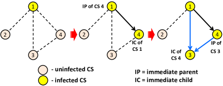
Figure 1: Example of type 1 and 2 CSes.

Initially, CS 1 is the lone failed CS and, as a result, CSes 2 through 4 face the possibility of infection by CS 1. Suppose that CS 4 becomes infected while CSes 2 and 3 remain unaffected. Since CS 4 has a single parent, namely CS 1, it is an example of type 1 CS. In this case, we call CS 4 an immediate child of CS 1, and refer to CS 1 as the immediate parent of CS 4.

On the other hand, even though CS 3 first survives the failure of CS 1, once CS 4 fails following its infection by CS 1, the failures of CSes 1 and 4, both of which are neighbors of CS 3, lead to that of CS 3. In this case, because it takes the failures of two neighbors to cause that of CS 3, it is an example of type 2 CS. We call CS 1 and CS 4 the first parent and the immediate parent, respectively, of CS 3. Analogously, we call CS 3 an immediate child of CS 4 (but not of CS 1). It will be clear why we call CS 1 and CS 4 the immediate parent of CS 4 and CS 3, respectively, when we describe the multi-type branching process to approximate failure propagation in Section 5.

Before we proceed, in order to explain the role of triangles in failure propagation dynamics, we first describe several scenarios where the presence of triangles in the dependence graph does not affect the failure propagation dynamics. This will help us to isolate the cases of interest to us, in which the existence of triangles alters the way failures propagate.

Sc1. In the example shown in Fig. 1, we assumed that CS 1 is a parent of CS 4. Suppose instead that CSes 1 and 4 are not neighbors, but there are additional failed CS(es) between them forming a path from CS 1 to CS 4 in the infection graph. In this case, since CSes 1 and 4 are not neighbors, CSes 1, 3 and 4 do not form a triangle. Thus, whether or not we model triangles in the dependence graph would not affect the transmission of failure to CS 3.

Sc2. Even though in Fig. 1 we assumed that CS 4 was infected by CS 1 alone, it is also possible that CS 4 has additional parent(s) that contributed to its failure. From the viewpoint of modeling the influence of the triangle (amongst CSes 1, 3, and 4) on potential infection of CS 3 by CSes 1 and 4, however, whether or not CS 4 has additional parent(s) is unimportant.

Sc3. According to the way we defined our infection graphs, three failed CSes that form a triangle in the dependence graph may not form a triangle in the undirected infection graph. The reason for this is that, when two neighboring CSes fail nearly simultaneously in such a way that the failure of one does not contribute to that of the other, there is no edge in the infection graph. Roughly speaking, there are two different ways in which this can happen.

1. One CS fails first and infects the other two neighbors that fail almost simultaneously, so that the latter two do not contribute to the failure of each other.

2. Two of the CSes first fail nearly at the same time in a way that the failure of one does not contribute to that of the other. These two failed CSes then cause the third CS to fail.

In case C1, the existence of the triangle in the dependence graph among the three CSes does not play any role in the propagation of failures and the infection of the latter two CSes would behave the same way even if they were not neighbors with each other. Similarly, in case C2, the existence of a triangle, more specifically that of an edge between the first two failing CSes, is irrelevant to the infection of the third CS.

These observations suggest that, from the viewpoint of modeling the effects of triangles in failure propagation, the only case in which the presence of a triangle among three CSes matters for transmitting failures is when the three CSes fail one after another and each failed CS contributes to ensuing failures of other CS(es). In other words, the first CS to fail contributes to the failure of the second CS in the triangle, and the failures of the first two CSes subsequently cause that of the third CS. This is precisely what our model captures as explained in the subsequent section.

Recall from scenario Sc1 that two failed neighbors of an uninfected CS might not be neighbors with each other. Therefore, in general the parents of a type 2 CS need not be neighbors. When this is true, however, the three CSes do not form a triangle and whether or not we model triangles would not have any significant impact on our study. Furthermore, if only a small fraction of CSes become infected as we assumed earlier, for most CSes with small to moderate degrees, the likelihood that they will have two or more failed neighbors that are not neighbors with each other would be small. For these reasons, we do not consider or model the scenarios where the two parents of a type 2 CS are not neighbors. Put differently, we only model type 2 CSes whose parents are neighbors and the three CSes form a triangle as illustrated in Fig. 1, in order to examine the effects of triangles in the dependence graph.

However, it should be evident that our model can be extended to consider other features, including larger cycles, by introducing additional types of CSes necessary to capture their presence. Obviously, this is likely to increase its complexity and degrade its tractability.

4.3 Infection probability of neighbors

For $t\in{\mathcal{T}}$, we denote by $q_{t}$ the probability that a CS (without knowing its degree) will fail following the $t$-th failure among the neighbors and become a type $t$ CS. We shall refer to $q_{t}$ as the infection probability of type $t$ CS. Keep in mind that these infection probabilities $q_{t}$, $t\in{\mathcal{T}}$, do not depend on clustering coefficient as we explain below.

$\bullet$ Computation of $q_{1}$: The infection probability $q_{1}$ is the probability with which CS 4 (or CS 2 or 3) is infected by CS 1 as the sole failed neighbor in Fig. 1 without knowing the degree of CS 4. According to the model outlined in Section 3.2, a CS of degree $d$ with only a single failed neighbor will fail with probability $\wp_{f}(d,1)$. Therefore, by conditioning on the degree of the neighbor, we can obtain the infection probability $q_{1}$ as

$$q_{1} := \sum_{d\in{\rm I\kern-1.5ptN}}w_{1}(d)\ \wp_{f}(d,1),$$ (2)

where

$$w_{1}(d):=\frac{d\cdot p_{0}(d)}{d_{{\rm avg}}}\ \mbox{ for all }\ d\in{\rm I\kern-1.5ptN},$$ (3)

and $d_{{\rm avg}}:=\sum_{d\in{\rm I\kern-1.5ptN}}d\cdot p_{0}(d)$ is the average degree of CSes.

The reason that the degree distribution of a neighbor used in (2) is given by ${\bf w}_{1}:=(w_{1}(d);\ d\in{\rm I\kern-1.5ptN})$, as opposed to ${\bf p}_{0}$, was first discussed in [10]: the degree distribution of the neighbor is the conditional degree distribution given that it is a neighbor of the failed CS attempting to infect it. The probability that a neighbor of the failed CS has degree $d$ is proportional to $d$ and, hence, is approximately $w_{1}(d)$ under the assumption that the dependence graph is neutral.

$\bullet$ Computation of $q_{2}$: The infection probability $q_{2}$ can be computed in an analogous manner. Since $q_{2}$ is the probability that a CS fails following the second failure among neighbors and we assume that the two failed neighbors form a triangle with the CS (from the previous subsection), this is the probability with which CS 3 fails in the example of Fig. 1, following the failure of CS 4 after having survived the failure of CS 1 (without knowing the degree of CS 3). First, since the CS has two failed neighbors, clearly its degree is at least two. Second, it must have survived the first failure of a neighbor before succumbing to the second failure among neighbors.

Because the degree of such a CS cannot be one, the conditional degree distribution is given by ${\bf w}_{2}:=(w_{2}(d);\ d\in{\rm I\kern-1.5ptN})$, where

$$w_{2}(1)=0\ \mbox{ and }\ w_{2}(d)=\frac{w_{1}(d)}{1-w_{1}(1)}\ \mbox{ for }\ d\in{\rm I\kern-1.5ptN}\setminus\{1\}.$$ (4)

Taking these observations into account and conditioning on the degree of CS, we obtain

$$q_{2} := \sum_{d\in{\rm I\kern-1.5ptN}}w_{2}(d)(1-\wp_{f}(d,1))\tilde{\wp}_{f}(d,2),$$ (5)

where $\tilde{\wp}_{f}(d,2)$ is the probability that a CS of degree $d$ will fail after the second failure among neighbors, conditional on that it survived the first failure of a neighbor. Using the definition of the conditional probability, we get

$$\tilde{\wp}_{f}(d,2) := \frac{\wp_{f}(d,2)-\wp_{f}(d,1)}{1-\wp_{f}(d,1)},\ d\in{\rm I\kern-1.5ptN}\setminus\{1\}.$$ (6)

Substituting (4) and (6) in (5), we get

$$q_{2} = \frac{1}{1-w_{1}(1)}\sum_{d=2}^{\infty}w_{1}(d)\big{(}\wp_{f}(d,2)-\wp_{f}(d,1)\big{)}.$$ (7)

Let us explain the conditional probability $\tilde{\wp}_{f}(d,2)$ given in (6) using the Watts’ model. As explained earlier, a CS fails when the fraction of failed neighbors exceeds its security state $\xi$ and $\wp_{f}(d,n_{f})=F(n_{f}/d)$. Therefore, given that a CS of degree $d$ survived the failure of a single neighbor, the conditional probability that it will fail when a second neighbor fails is equal to

$$\tilde{\wp}_{f}(d,2) = {\mathbbm{P}}\left[\xi<\frac{2}{d}\ \Big{|}\ \xi\geq\frac{1}{d}\right]=\frac{{\mathbbm{P}}\left[\frac{1}{d}\leq\xi<\frac{2}{d}\right]}{{\mathbbm{P}}\left[\frac{1}{d}\leq\xi\right]}$$

$$= \frac{\wp_{f}(d,2)-\wp_{f}(d,1)}{1-\wp_{f}(d,1)}.$$

From the degree distributions defined in (3) and (4) and used to compute the infection probabilities in (2) and (5), respectively, it is clear that our model implicitly assumes a neutral dependence graph and does not model any potential degree correlations between CSes. It has been observed (e.g., [19, 32]) that one of challenges to studying the effects of clustering is that, many existing models for generating clustered networks unintentionally introduce degree correlations or assortativity. From the construction of cliques via replication of nodes with identical degrees, it is obvious that similar degree correlations are introduced in the model proposed in [15, 16].

In [32], Miller points out that the influence of such degree correlations caused some researchers to incorrectly conclude that clustering facilitates cascades of failures with respect to cascade sizes and cascade threshold; he demonstrates that, when compared against unclustered networks with similar degree correlations, clustered networks have smaller cascade sizes and higher cascade threshold. In other words, clustering has the opposite effects and impedes cascades of failures.

Our model does away with this problem by modeling the influence of clustering on transmission of failures, rather than trying to generate random graphs (of finite size) explicitly. For this reason, any qualitative changes in the robustness of systems we identify using the model can be attributed to clustering, without having to worry about the influence of degree correlations.

5 Multi-type Branching Process for Modeling the Spread of Failures

We approximate the propagation of failures among CSes using a multi-type branching process (MTBP), in which the members of the MTBP are of the types defined in the previous section. We estimate the PoCF of a large system, using the probability that the population in the MTBP does not die out.

This approach is consistent with our notion of cascading failures provided in Section 1: when cascading failures occur in a large system, they will likely spread to different parts of the system well beyond the local neighborhood near the initial random failure and slow down only when newly failed CSes do not have neighbors to infect any more. Thus, in the case of an infinite network where the number of CSes in the system is unbounded (as assumed in many studies, e.g., [19, 29, 32, 48]), the spread of failures will not cease when cascading failures happen, which is equivalent to the population not dying out in our MTBP.

We assume that initially a randomly chosen CS experiences a failure. Since this CS does not have any parent, it is of type 0. Subsequently, when a type $t$ CS fails, it produces immediate children of two different types in accordance with the (immediate) children distribution $h_{t}$ described below, independently of other infected CSes in the system.

5.1 Multi-type branching processes

The MTBP we use to approximate failure propagation can be constructed as follows: it starts with a single type 0 agent at the beginning (the zero-th generation). Then, each member in the $k$-th generation ($k\in{\mathbbm{Z}}_{+}$) produces immediate children of two different types, who become members of the $(k+1)$-th generation, according to children distributions derived in Section 5.2, independently of each other.

Since an infected CS can have up to two parents and, when a CS has two parents, one of them is the parent of the other as shown in Fig. 1, the parents themselves can belong to two different generations. A failed CS in our infection graph belongs to the $k$-th generation in the MTBP if and only if the length of the longest path in the infection graph from the root to the CS is equal to $k$.

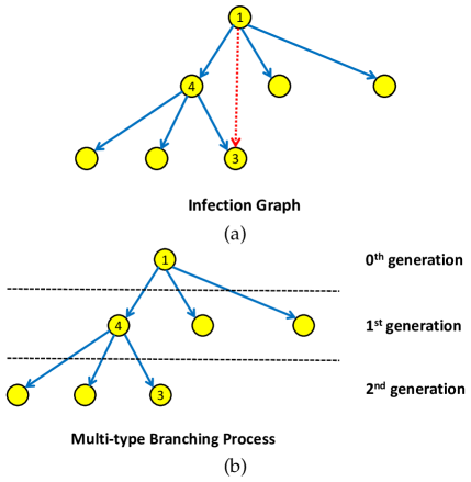
Figure 2: (a) Infection graph, (b) corresponding Multi-type branching process.

Let us illustrate this using the example in Fig. 1 with CS 1 as the root of an infection graph, which experiences the first failure. The resulting infection graph is shown in Fig. 2(a), where unnumbered circles are other infected children that are not shown in Fig. 1. In the figure, a solid blue arrow indicates the influence of the immediate parent that causes the child to fail, whereas a dotted red arrow represents the influence of the first parent of a type 2 CS which contributes to the failure.

In order to construct the corresponding MTBP, we only keep the solid blue arrows and delete the dotted red arrows from the infection graph. In other words, we only retain the arrows from immediate parents. Since every CS has a single (immediate) parent in the new graph, it is clear that this gives rise to a directed tree. This is shown in Fig. 2(b). A failed CS is now a member of the $k$-th generation in MTBP if its distance from the root in this new tree is $k$.

5.2 Immediate children distributions in MTBPs

In order to complete the description of the MTBP that we employ to approximate failure propagation, we need to specify the children distribution for each type. Clearly, except for the initial CS that experiences a random failure, which is the root of the infection graph, all other infected CSes are of type 1 or 2, because they must have a parent. Thus, all children infected by a failed CS would be of either type 1 or 2.

$\bullet$ Neighbors of a type 0 CS: Assume that CS $a$ experiences the initial random failure. Since CS $a$ is the only failed CS at the moment, all of its neighbors face the risk of infection from a single neighbor. Thus, each neighbor will be infected by CS $a$ and become its immediate child with probability $q_{1}=:v^{C}_{0,1}$ or remain unaffected with probability $1-q_{1}=:v^{C}_{0,0}$.

Because of the presence of triangles in the dependence graph, it is possible that some of immediate children of CS $a$ are also neighbors of other unaffected neighbors of CS $a$. Suppose that one of these unaffected neighbors of CS $a$ fails as a result of the failure of a second neighbor, say CS $a^{\prime}$, which was infected by CS $a$. Then, it will be an immediate child of CS $a^{\prime}$ and will not count as an immediate child of CS $a$, as explained in Section 4.2.

$\bullet$ Neighbors of a type 1 CS: Suppose that a CS $a$ is infected by a single parent $a^{\prime}$ and, hence, is of type 1. Recall from the definition in (1) that the clustering coefficient is the likelihood that there is an edge between the two neighbors of a connected triple. Thus, when the clustering coefficient is $C\in(0,1)$, the probability that there is an edge between a randomly chosen neighbor of $a$ and its parent $a^{\prime}$ can be approximated using $C$ because CS $a$ is a connected triple. Moreover, we assume that each neighbor of $a$ has an edge with the parent $a^{\prime}$ with probability $C$, independently of each other, which is reasonable for large systems.

Based on this assumption, we approximate the probability that a neighbor becomes another type 1 CS using the product $(1-C)q_{1}=:v^{C}_{1,1}$ of (a) the probability that it is not a neighbor of $a^{\prime}$ ($1-C$) and (b) that of becoming infected by the failure of CS $a$ ($q_{1}$). Similarly, the probability that the neighbor has an edge with $a^{\prime}$ and becomes a type 2 CS is estimated using $C\cdot q_{2}=:v^{C}_{1,2}$. Note that, when the neighbor has an edge with the parent $a^{\prime}$, in order for it to be a type 2 CS, it must have initially survived the failure of $a^{\prime}$ and then fail following the failure of CS $a$. Hence, the probability that it will fail following the infection of CS $a$ and become a type 2 CS would be $q_{2}$, not $q_{1}$, as explained in Section 4.3. Finally, the probability that it remains unaffected is $1-(1-C)q_{1}-C\cdot q_{2}=:v^{C}_{1,0}$.

$\bullet$ Neighbors of a type 2 CS: When CS $a$ is of type 2 with two parents, it is possible for a neighbor of CS $a$ to have an edge with both of the parents and, thus, have three failed neighbors. However, when the fraction of failed CSes is low or the clustering coefficient $C$ is not large, this would not occur often. Furthermore, modeling CSes with more than two infected neighbors would require introducing additional types of CSes. For these reasons, we do not explicitly model the cases where a CS faces more than two failed neighbors and approximate them using the case where the CS has only two failed neighbors instead.

Making use of this argument, we assume that neighbors of a type 2 CS have an edge with (a) neither parent with probability $(1-C)^{2}$ and (b) one parent with probability $1-(1-C)^{2}=(2C-C^{2})$, independently of each other. Note that the possibility of being a neighbor with both parents is folded into the latter scenario of having an edge with only one parent.

On the basis of this assumption, we estimate the probability that a neighbor of CS $a$ becomes a type 1 CS using $(1-C)^{2}q_{1}=:v^{C}_{2,1}$ and that of becoming a type 2 CS by $(2C-C^{2})q_{2}=:v^{C}_{2,2}$. Finally, the probability that the neighbor avoids infection is equal to $1-(1-C)^{2}q_{1}-(2C-C^{2})q_{2}=:v^{C}_{2,0}$. When it is convenient and there is no risk of confusion, we do not explicitly denote the dependence on clustering coefficient $C$ and write $v_{t,t^{\prime}}$ in place of $v^{C}_{t,t^{\prime}}$.

5.2.1 Conditional degree distributions of failed CSes

Given these probabilities, once we fix the degree $d$ and type $t$ of a failed CS, we can approximate the distribution of the number of immediate children of different types, which are produced by the CS with the help of multinomial distributions: the probability that it produces $o_{1}$ type 1 children and $o_{2}$ type 2 children (with $o_{1}+o_{2}\leq d-t$) is given by

$$\left[\frac{d-t}{o_{1}:o_{2}}\right]v_{t,1}^{o_{1}}\ v_{t,2}^{o_{2}}\ v_{t,0}^{d-t-o_{1}-o_{2}},$$

where $v_{0,2}=0$, and

$$\left[\frac{d-t}{o_{1}:o_{2}}\right]:=\frac{(d-t)!}{o_{1}!o_{2}!(d-t-o_{1}-o_{2})!},$$

denotes a multinomial coefficient. Hence, we can estimate the children distribution by conditioning on the degree of the CS.

The conditional degree distributions of infected CSes in general differ from the prior distribution ${\bf p}_{0}$. We denote the conditional degree distribution of type $t$ CSes by ${\bf p}_{t}:=(p_{t}(d);\ d\in{\rm I\kern-1.5ptN})$, $t\in{\mathcal{T}}$. Making use of the degree distributions of neighbors defined in (3) and (4) and the failure probability function $\wp_{f}$, we can obtain the following conditional degree distributions of infected CSes:

$$p_{1}(d) = \frac{w_{1}(d)\ \wp_{f}(d,1)}{q_{1}}\ \mbox{ for }d\in{\rm I\kern-1.5ptN},$$

$$p_{2}(d) = \frac{w_{1}(d)(\wp_{f}(d,2)-\wp_{f}(d,1))}{(1-w_{1}(1))q_{2}}\ \mbox{ for }d\in{\rm I\kern-1.5ptN}\setminus\{1\},$$

and $p_{2}(1)=0$.

5.2.2 Children distributions

Putting all the pieces together, we acquire the following (immediate) children distributions for different types: fix clustering coefficient $C\in(0,1)$. The probability that a CS of type $t\in\{0,1,2\}$ will produce immediate children given by a children vector ${\bf o}=(o_{1},o_{2})\in{\mathbbm{Z}}_{+}^{2}$, where $o_{j}$ is the number of type $j$ immediate children, is given by

$$h_{t}({\bf o};C)$$ (8)

$$= \sum_{\tau=o_{1}+o_{2}}^{\infty}\Big{(}p_{t}(\tau+t)\ \left[\frac{\tau}{o_{1}:o_{2}}\right]v_{t,1}^{o_{1}}\ v_{t,2}^{o_{2}}\ v_{t,0}^{\tau-o_{1}-o_{2}}\Big{)}.$$

5.3 Probability of extinction

Let $N_{t}(k)$, $t\in{\mathcal{T}}$ and $k\in{\rm I\kern-1.5ptN}$, be the number of type $t$ CSes in the $k$-th generation of the MTBP. For instance, in Fig. 2(b), $N_{1}(1)=3$, $N_{2}(1)=0$, $N_{1}(2)=2$, and $N_{2}(2)=1$. The probability ${\mathbbm{P}}\left[\limsup_{k\to\infty}\ (N_{1}(k)+N_{2}(k))=0\right]$ is called the probability of extinction (PoE) [20]. Obviously, the PoCF is equal to one minus the PoE.

Let $\bm{\mu}=(\mu_{1},\mu_{2})$, where $\mu_{t}$ is the PoE, starting with a single type $t$ infected CS (instead of a type 0 CS). The probability of interest to us is the PoE starting with a single type 0 CS, which we denote by $\mu_{0}$. This can be computed from $\mu_{1}$ by conditioning on the degree of the CS, say $a$, which experiences the initial random failure. In other words,

$$\mu_{0} = \sum_{d\in{\rm I\kern-1.5ptN}}p_{0}(d)\big{(}1-q_{1}(1-\mu_{1})\big{)}^{d}.$$ (9)

Note that $q_{1}(1-\mu_{1})$ is the probability that a neighbor of CS $a$ will be infected and then trigger a cascade of failures. Thus, $(1-q_{1}(1-\mu_{1}))^{d}$ is the probability that none of the $d$ neighbors gives rise to cascading failures. A key question of interest to us is how clustering coefficient $C$ affects the PoE $\mu_{0}$ defined in (9), which is a strictly increasing function of $\mu_{1}$.

For each $t\in{\mathcal{T}}$, let ${\mathbbm{E}}\left[h_{t}\right]=({\mathbbm{E}}\left[h_{t,t^{\prime}}\right];\ t^{\prime}\in{\mathcal{T}})$ be a $1\times 2$ row vector, whose $t^{\prime}$-th element is the expected number of type $t^{\prime}$ immediate children from a type $t$ CS. Define ${\mathbbm{M}}=[M_{t,t^{\prime}}]$ to be a $2\times 2$ matrix, whose $t$-th row is ${\mathbbm{E}}\left[h_{t}\right]$, i.e., $M_{t,t^{\prime}}={\mathbbm{E}}\left[h_{t,t^{\prime}}\right]$ for all $t,t^{\prime}\in{\mathcal{T}}$. Let $\rho({\mathbbm{M}})$ denote the spectral radius of ${\mathbbm{M}}$ [21].

It is well known [20] that $\bm{\mu}={\bf 1}$ if (i) $\rho({\mathbbm{M}})<1$ or (ii) $\rho({\mathbbm{M}})=1$ and there is at least one type for which the probability that it produces exactly one child is not equal to one. Similarly, if $\rho({\mathbbm{M}})>1$, then $\bm{\mu}<{\bf 1}$ and there is strictly positive probability that spreading failures continue forever in an infinite system, suggesting that there could be a cascade of failures in a large system.

6 Main Analytical Result

As stated in Section 1, our goal is to understand how clustering among CSes in the dependence graph affects the robustness of the system. As it will be clear, the relation between the PoCF (or equivalently, PoE) and system parameters, including clustering coefficient, is rather complicated. In particular, our main finding stated in Theorem 1 below suggests that whether increasing clustering escalates the PoE or not depends on the infection probabilities $q_{1}$ and $q_{2}$ and the current PoEs $\mu_{1}$ and $\mu_{2}$.

Theorem 1

Suppose $0<C_{1}<C_{2}<1$ and let $\bm{\mu}^{i}=(\mu^{i}_{1},\mu^{i}_{2})$, $i=1,2$, be the PoE vector corresponding to clustering coefficient $C_{i}$. Assume that $\bm{\mu}^{1}<{\bf 1}$. Then, $\bm{\mu}^{1}\leq\bm{\mu}^{2}$ if $(1-\mu^{1}_{1})q_{1}\geq(1-\mu^{1}_{2})q_{2}$. Analogously, we have $\bm{\mu}^{1}\geq\bm{\mu}^{2}$ if $(1-\mu^{1}_{1})q_{1}\leq(1-\mu^{1}_{2})q_{2}$.

Proof:

A proof is provided in Section 8. ∎

The theorem suggests that the relation between clustering coefficient and PoCF is far from simple in that it depends on many factors, including the degree distribution ${\bf p}_{0}$ and the failure probability function $\wp_{f}$, in a rather subtle fashion. At the same time, it hints that their effects can be succinctly summarized by the terms in the condition, namely the current PoEs $\mu_{t}$, $t\in{\mathcal{T}}$, and infection probabilities $q_{t}$, $t\in{\mathcal{T}}$.

Before we proceed with our discussion, let us first rewrite the conditions in the theorem in a slightly different manner:

$$\frac{1-\mu^{1}_{1}}{1-\mu^{1}_{2}}\geq\frac{q_{2}}{q_{1}}\mbox{ and }\frac{1-\mu^{1}_{1}}{1-\mu^{1}_{2}}\leq\frac{q_{2}}{q_{1}}$$ (10)

Remark 1. Recall that $1-\mu_{t}$ is the PoCF starting with a single type $t$ CS. Thus, $(1-\mu_{1})/(1-\mu_{2})$ is the ratio of the PoCFs starting with two different types of CSes. It is now clear that the conditions in the theorem compare the ratio of PoCFs for two different types of CSes to that of infection probabilities. While one would expect the ratio of infection probabilities to play a role, to the best of our knowledge, our result is the first to bring to light (i) the fact that the ratio of PoCFs, $(1-\mu_{1})/(1-\mu_{2})$, plays a similar/important role and (ii) a condition that tells us when increasing clustering improves or degrades the robustness of the system.

Remark 2. A key implication of our finding is the following: consider two distinct degree distributions with the same mean, but one degree distribution is more concentrated (around the mean) with smaller variance than the other. As the clustering coefficient becomes larger, the fraction of type 2 CSes tends to increase. Because a type 2 CS already has two failed neighbors compared to a single failed neighbor of a type 1 CS, when CS degrees are concentrated (around the mean degree), a type 2 CS has fewer neighbors that it can potentially infect, thereby producing a smaller number of children on the average.

A consequence of this is that it leads to higher concentration of failed CSes in a local neighborhood. At the same time, it hinders spreading failures beyond the local neighborhood of already failed CSes, especially when the mean degrees are not large. Moreover, as we will demonstrate in the subsequent section, clustering has more pronounced impact on PoCFs.

Remark 3. One important fact we should point out is that Theorem 1 alone does not guarantee the monotonicity of PoE (equivalently, PoCF) with respect to clustering coefficient. The reason for this is as follows: suppose that $0<C_{1}<C_{2}<C_{3}<1$ and $\bm{\mu}^{i}$ is the PoE vector corresponding to $C_{i}$, $i=1,2,3$. Then, it is possible to have $\frac{1-\mu^{1}_{1}}{1-\mu^{1}_{2}}>\frac{q_{2}}{q_{1}}$ while $\frac{1-\mu^{2}_{1}}{1-\mu^{2}_{2}}<\frac{q_{2}}{q_{1}}$ because the PoEs can change when the clustering coefficient goes up from $C_{1}$ to $C_{2}$. When this happens, Theorem 1 tells us (i) $\bm{\mu}^{1}\leq\bm{\mu}^{2}$ and $\bm{\mu}^{1}\leq\bm{\mu}^{3}$ from the first inequality and (ii) $\bm{\mu}^{2}\geq\bm{\mu}^{3}$ from the second inequality. Thus, in principle, we could end up with $\bm{\mu}^{1}<\bm{\mu}^{3}<\bm{\mu}^{2}$. However, our numerical studies provided in the subsequent section indicate that the monotonicity of PoCF may hold in many cases of practical interest.

7 Numerical Results

Our main result in Section 6 tells us that, once we know the PoEs $\mu_{t}$, $t\in{\mathcal{T}}$, and the infection probabilities $q_{t}$, $t\in{\mathcal{T}}$, for a fixed clustering coefficient, we can determine whether an increasing clustering coefficient will elevate or lower the resulting PoCF. But, this requires the knowledge of, among other things, the infection probabilities $q_{t}$, $t\in{\mathcal{T}}$, which depend on the degree distribution in the dependence graph and failure probability function $\wp_{f}$.

The goal of this section is to provide numerical results to examine how various parameters in our analysis are affected by the clustering coefficient as we change the degree distribution and the failure probability function. To this end, we vary the clustering coefficient over [0.025, 0.40], under two commonly studied degree distributions – power law degree distributions and Poisson degree distributions.

For our study, we consider failure probability functions of the form $\wp_{f}(d,n_{f})=(n_{f}/d)^{\alpha}$ with $\alpha\in[0.6,1.0]$. When $\alpha$ is small, even the failure of a single neighbor causes the failure of a CS with relatively high probability. In this sense, $\wp_{f}(d,n_{f})$ is less sensitive to $d$. On the other hand, for large $\alpha$, many neighbors have to fail first before a CS fails as a result. Throughout the section, we assume that the largest degree of a CS is 20, which we denote by $D_{\max}$, and define ${\mathcal{D}}:=\{1,2,\ldots,D_{\max}\}$.

7.1 Power law degree distributions

Power law degree distributions assume $p_{0}(d)\propto d^{-\beta}$ for some positive constant $\beta$. For many real networks, the power law exponent $\beta$ lies between 2 and 4 [1, 30]. In our study, we considered $\beta\in[1.5,4]$. However, for $\beta>2.5$, the resulting PoCF is very small and, for this reason, we do not present the numbers here.

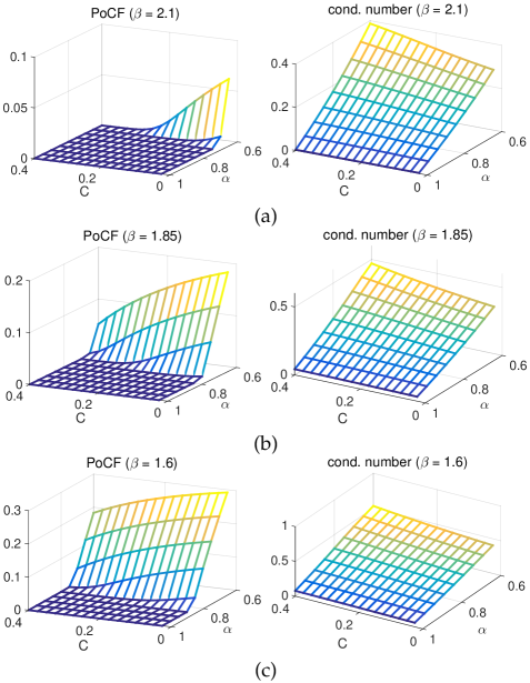
Figure 3: Plots of PoCFs and condition numbers with power law degree distributions. (a) $\beta=2.1$, (b) $\beta=1.85$, and (c) $\beta=1.6$.

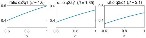
Figure 4: Ratios of infection probabilities.

Fig. 3 plots the PoCF (i.e., $1-\mu_{0}$) and the condition number as a function of the failure probability function parameter $\alpha$ and clustering coefficient $C$ for three different values of power law exponent $\beta$ – 1.6, 1.85 and 2.1. Here, the condition number refers to the difference $\frac{1-\mu_{1}}{1-\mu_{2}}-\frac{q_{2}}{q_{1}}$. The average degree of CSes under the three values of $\beta$ is 3.186, 2.548, and 2.089, respectively. As mentioned earlier, while we examined the scenarios with larger $\beta$, the PoCF was too small to be of much interest in our opinion.

O1. According to Theorem 1, when the condition number is positive (resp. negative), increasing clustering coefficient $C$ reduces (resp. elevates) the PoCF. It is clear from Fig. 3 that, for all three values of $\beta$, the condition number is always positive, and the PoCF decreases with clustering coefficient $C$. Hence, the plots corroborate our finding in the theorem. Furthermore, they suggest that the system is likely to become more robust against random failures and less prone to experience a cascade of failures. This observation is consistent with the findings of [32, 47], which reported that clustering has an effect of impeding cascades of diseases or information.

O2. Fig. 4 shows that the ratio of infection probabilities ($q_{2}/q_{1}$) never exceeds one. This is in part a consequence of the following two observations: (i) a potential type 2 CS (i.e., a CS with two failed neighbors) has a larger degree (with respect to the usual stochastic order) than those facing a single failed neighbor (${\bf w}_{2}$ vs. ${\bf w}_{1}$); and (ii) with the assumed infection probability function $\wp_{f}$, it becomes more difficult to infect CSes with two failed neighbors, which already survived the first failure of a neighbor, than to infect CSes facing the risk of infection from a single failed neighbor. This can be seen from the inequality $\wp_{f}(d,2)-\wp_{f}(d,1)=\frac{1}{d^{\alpha}}(2^{\alpha}-1)\leq\frac{1}{d^{\alpha}}$ because $2^{\alpha}\leq 2$ for $\alpha\leq 1$.

O3. It is evident from Fig. 4 that the ratio of infection probabilities ($q_{2}/q_{1}$) increases with the parameter $\alpha$. The reason for this is that, for the assumed infection probability function, we have

$$\frac{\wp_{f}(d,2)-\wp_{f}(d,1)}{\wp_{f}(d,1)} = \frac{d^{-\alpha}(2^{\alpha}-1)}{d^{-\alpha}}=2^{\alpha}-1$$

for all $d>1$, which increases with $\alpha$. Thus, from the definition of $q_{1}$ and $q_{2}$ in (2) and (7), respectively, it is obvious that the ratio $q_{2}/q_{1}$ will follow the same trend.

7.2 Poisson degree distributions

When CS degrees are Poisson distributed with parameter $\lambda>0$, $p_{0}(d)\propto\frac{\lambda^{d}}{d!}$ for all $d\in{\mathcal{D}}$. A key difference from power law distributions is that a Poisson distribution is more concentrated around its mean value. For our study, we consider $\lambda\in$ [2.0, 4.5].

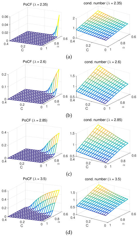
Figure 5: Plots of PoCFs and condition numbers under Poisson degree distributions. (a) $\lambda=2.35$, (b) $\lambda=2.6$, (c) $\lambda=2.85$ and (d) $\lambda=3.5$.

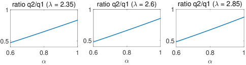
Figure 6: Ratios of infection probabilities.

Fig. 5 plots the PoCF and the condition number for $\lambda=$ 2.35, 2.6, 2.85, and 3.5. The corresponding average degrees are 2.598, 2.809, 3.025, and 3.609, respectively. From the plots, we can draw the following observations.

O4. Similar to the plots in Fig. 3 under power law degree distributions, the PoCF tends to decrease with increasing clustering. This can be also inferred from positive condition numbers shown in Fig. 5.

One noticeable difference is that comparing Fig. 5 to Fig. 3 reveals that the PoCF is much more sensitive and decreases more rapidly with increasing clustering. This is a direct consequence of the earlier observations that (i) CS degrees are concentrated around the mean value under Poisson degree distributions and (ii) when CS degrees are more concentrated around the mean value, the clustering tends to impede cascading failures and have greater influence on PoCFs, especially with small mean degrees (which lie between 2.598 and 3.609 for scenarios shown in Fig. 5).

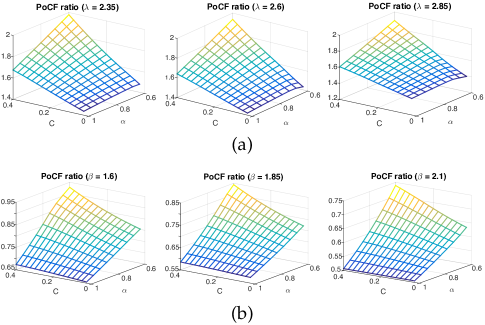
Figure 7: Ratios of PoCFs $(1-\mu_{1})/(1-\mu_{2})$. (a) Poisson degree distributions for $\lambda=$ 2.35, 2.6, and 2.85, (b) power law degree distribution for $\beta=$ 1.6, 1.85, and 2.1.

O5. Comparing the condition numbers in Figs. 3 and 5 and the infection probability ratios in Figs. 4 and 6, we can see that both the condition numbers and the infection probability ratios are considerably larger with Poisson degree distributions. This tells us that the ratio of PoCFs given by $\frac{1-\mu_{1}}{1-\mu_{2}}$, which equals the sum of the first two ratios, is larger than one with Poisson degree distributions. This is shown in Fig. 7(a). Therefore, it corroborates Remark 2 in the previous section that, when the degree distribution is concentrated, a type 1 CS is more effective at triggering cascading failures than a type 2 CS.

Let ${\mathbbm{E}}\left[{\bf p}_{t}\right]$, $t\in{\mathcal{T}}$, be the average degree among type $t$ CSes. Given that $q_{2}<q_{1}$ as shown in Fig. 6, if ${\mathbbm{E}}\left[{\bf p}_{2}\right]-{\mathbbm{E}}\left[{\bf p}_{1}\right]<1$, clearly a type 1 CS would serve as a better trigger than a type 2 CS because, together, they imply that a type 1 CS on the average generates (i) more type 1 children and (ii) a larger number of immediate children. It turns out that the difference ${\mathbbm{E}}\left[{\bf p}_{2}\right]-{\mathbbm{E}}\left[{\bf p}_{1}\right]$ is (considerably) less than one in the cases we considered. For example, for $\alpha=0.6$ and $\lambda=2.35$ (resp. $\alpha=0.8$ and $\lambda=2.85$), we have ${\mathbbm{E}}\left[{\bf p}_{1}\right]=2.899$ and ${\mathbbm{E}}\left[{\bf p}_{2}\right]=3.303$ (resp. ${\mathbbm{E}}\left[{\bf p}_{1}\right]=3.194$ and ${\mathbbm{E}}\left[{\bf p}_{2}\right]=3.562$).

Carrying out the same exercise for power law degree distributions illustrates that the ratio of PoCFs $\big{(}\frac{1-\mu_{1}}{1-\mu_{2}}\big{)}$ is less than one, as shown in Fig. 7(b). Thus, in this case, the opposite is true, and a type 2 CS is more likely to trigger a cascade of failures than a type 1 CS. This can be in part attributed to the following observation:

Substituting the expressions for the power law degree distributions and the assumed failure probability function in the expressions for the conditional degree distributions ${\bf p}_{t}$ yields

$$p_{t}(d) \propto d^{-(\beta+\alpha-1)}\ \mbox{ for all }\ t\leq d\leq D_{\max}.$$ (11)

From (11), because the conditional degree distribution does not decrease quickly (e.g., exponentially) with $d$, the difference ${\mathbbm{E}}\left[{\bf p}_{2}\right]-{\mathbbm{E}}\left[{\bf p}_{1}\right]$ tends to be larger than one. For instance, for $\alpha=0.8$ and $\beta=1.6$ (resp. $\alpha=0.6$ and $\beta=1.85$), we have ${\mathbbm{E}}\left[p_{1}\right]=3.846$ and ${\mathbbm{E}}\left[p_{2}\right]=5.941$ (resp. ${\mathbbm{E}}\left[p_{1}\right]=3.668$ and ${\mathbbm{E}}\left[p_{2}\right]=5.785$). Therefore, this suggests that, at least for small clustering coefficient $C$, a type 2 CS is more likely to be successful at setting off cascading failures than a type 1 CS because its (expected) degree is much larger.

8 A proof of Theorem 1

For each $t\in{\mathcal{T}}$, define a generating function $f_{t}:[0,1]^{3}\to[0,1]$, where

$$f_{t}(s_{1},s_{2};C)=\sum_{(o_{1},o_{2})\in{\mathbbm{Z}}_{+}^{2}}h_{t}(o_{1},o_{2};C)\ s_{1}^{o_{1}}\ s_{2}^{o_{2}}.$$ (12)

Then, for a fixed clustering coefficient $C\in(0,1)$, the PoE vector $\bm{\mu}$ is given as a fixed point that satisfies

$${\bf f}(\bm{\mu};C) = \bm{\mu}\leq{\bf 1},$$ (13)

where ${\bf f}({\bf s};C)=(f_{1}({\bf s};C),f_{2}({\bf s};C))$. When $\rho({\mathbbm{M}})>1$, there exists a unique $\bm{\mu}$ that satisfies (13) with strict inequality, i.e., $\bm{\mu}<{\bf 1}$ [20].

In order to prove the theorem, we will first prove that, if $(1-\mu^{1}_{1})q_{1}\geq(1-\mu^{1}_{2})q_{2}$ (resp. $(1-\mu^{1}_{1})q_{1}\geq(1-\mu^{1}_{2})q_{2}$), then $\bm{\mu}^{1}\leq{\bf f}(\bm{\mu}^{1};C_{2})$ (resp. $\bm{\mu}^{1}\geq{\bf f}(\bm{\mu}^{1};C_{2})$). When this is true, Corollary 2 [20, p. 42] tells us that $\bm{\mu}^{1}\leq\bm{\mu}^{2}$ (resp. $\bm{\mu}^{1}\geq\bm{\mu}^{2}$), completing the proof.

Let us begin with the first part of the theorem. Recall from (8) and (12)

$$f_{1}({\bf s};C) = \sum_{{\bf o}\in{\mathbbm{Z}}_{+}^{2}}h_{1}({\bf o};C)\ s_{1}^{o_{1}}\ s_{2}^{o_{2}}$$

$$= \sum_{{\bf o}\in{\mathbbm{Z}}_{+}^{2}}s_{1}^{o_{1}}\ s_{2}^{o_{2}}\sum_{d\geq o_{1}+o_{2}+1}\Big{(}p_{1}(d)\left[\frac{d-1}{o_{1}:o_{2}}\right]$$

$$\hskip 21.68121pt\times(v^{C}_{1,1})^{o_{1}}\ (v^{C}_{1,2})^{o_{2}}\ (v^{C}_{1,0})^{d-o_{1}-o_{2}-1}\Big{)}.$$

After exchanging the order of the two summations, we obtain

$$f_{1}({\bf s};C)$$ (14)

$$= \sum_{d\in{\rm I\kern-1.5ptN}}p_{1}(d)\Big{(}\sum_{{\bf o}\in{\mathbbm{Z}}_{+}^{2}:o_{1}+o_{2}\leq d-1}s_{1}^{o_{1}}\ s_{2}^{o_{2}}\left[\frac{d-1}{o_{1}:o_{2}}\right]$$

$$\hskip 43.36243pt\times(v^{C}_{1,1})^{o_{1}}\ (v^{C}_{1,2})^{o_{2}}\ (v^{C}_{1,0})^{d-o_{1}-o_{2}-1}\Big{)}$$

$$= \sum_{d\in{\rm I\kern-1.5ptN}}p_{1}(d)\big{(}\underbrace{s_{1}\ v^{C}_{1,1}+s_{2}\ v^{C}_{1,2}+v^{C}_{1,0}}_{\text{ \large{$=:\psi_{1}({\bf s},C)$}}}\big{)}^{d-1}.$$

The second equality in (14) follows from the well-known equality

$$\sum_{\sum_{k=1}^{m}n_{k}=N}{{N}\choose{n_{1},n_{2},\ldots,n_{m}}}\prod_{k=1}^{m}\left(x_{k}\right)^{n_{k}} = \left(\sum_{k=1}^{m}x_{k}\right)^{N},$$

where the summation on the left-hand side is over non-negative integers $n_{k}$, $k=1,2,\ldots,m$, whose sum equals $N$. Following similar steps, we obtain

$$f_{2}({\bf s};C)=\sum_{{\bf o}\in{\mathbbm{Z}}_{+}^{2}}h_{2}({\bf o};C)\ s_{1}^{o_{1}}\ s_{2}^{o_{2}}$$ (15)

$$= \sum_{{\bf o}\in{\mathbbm{Z}}_{+}^{2}}s_{1}^{o_{1}}\ s_{2}^{o_{2}}\sum_{d\geq o_{1}+o_{2}+2}\Big{(}p_{2}(d)\left[\frac{d-2}{o_{1}:o_{2}}\right]$$

$$\hskip 21.68121pt\times(v^{C}_{2,1})^{o_{1}}\ (v^{C}_{2,2})^{o_{2}}\ (v^{C}_{2,0})^{d-o_{1}-o_{2}-2}\Big{)}$$

$$= \sum_{d=2}^{\infty}p_{2}(d)\Big{(}\sum_{{\bf o}\in{\mathbbm{Z}}_{+}^{2}:o_{1}+o_{2}\leq d-2}s_{1}^{o_{1}}\ s_{2}^{o_{2}}\left[\frac{d-2}{o_{1}:o_{2}}\right]$$

$$\hskip 43.36243pt\times(v^{C}_{2,1})^{o_{1}}\ (v^{C}_{2,2})^{o_{2}}\ (v^{C}_{2,0})^{d-o_{1}-o_{2}-2}\Big{)}$$

$$= \sum_{d=2}^{\infty}p_{2}(d)\big{(}\underbrace{s_{1}\ v^{C}_{2,1}+s_{2}\ v^{C}_{2,2}+v^{C}_{2,0}}_{\text{ \large{$=:\psi_{2}({\bf s},C)$}}}\big{)}^{d-2}.$$

It is clear from (14) that $f_{1}(\bm{\mu}^{1};C_{1})=\mu^{1}_{1}\leq f_{1}(\bm{\mu}^{1};C_{2})$ if and only if $\psi_{1}(\bm{\mu}^{1},C_{1})\leq\psi_{1}(\bm{\mu}^{1},C_{2})$. Substituting the expressions $v^{C}_{1,1}=(1-C)q_{1}$, $v^{C}_{1,2}=C\cdot q_{2}$ and $v^{C}_{1,0}=1-v^{C}_{1,1}-v^{C}_{1,2}$ from Section 5.2, we obtain

$$\psi_{1}({\bf s},C) = s_{1}(1-C)q_{1}+s_{2}Cq_{2}+1-(1-C)q_{1}-Cq_{2}.$$

Hence, after grouping only the terms containing $C$, we see that $\psi(\bm{\mu}^{1},C_{1})\leq\psi(\bm{\mu}^{1},C_{2})$ if and only if

$$(1-\mu^{1}_{1})q_{1}-(1-\mu^{1}_{2})q_{2}\geq 0.$$ (16)

We now proceed to demonstrate that $\mu^{1}_{2}=f_{2}(\bm{\mu}^{1};C_{1})\leq f_{2}(\bm{\mu}^{1};C_{2})$. From (15), it is obvious that this claim is true if and only if $\psi_{2}(\bm{\mu}^{1},C_{1})\leq\psi_{2}(\bm{\mu}^{1},C_{2})$. Recall $v^{C}_{2,1}=(1-C)^{2}q_{1}$, $v^{C}_{2,2}=C(2-C)q_{2}$ and $v^{C}_{2,0}=1-(1-C)^{2}q_{1}-C(2-C)q_{2}$. Plugging in these expressions in $\psi_{2}({\bf s};C)$,

$$\psi_{2}({\bf s},C) = s_{1}(1-C)^{2}q_{1}+s_{2}C(2-C)q_{2}$$

$$+1-(1-C)^{2}q_{1}-C(2-C)q_{2}$$

$$= 1-(1-C)^{2}q_{1}(1-s_{1})-C(2-C)q_{2}(1-s_{2}).$$

Collecting only the terms with $C$ in $\psi_{2}({\bf s},C)$, we get

$$C(2-C)\big{(}(1-s_{1})q_{1}-(1-s_{2})q_{2}\big{)}.$$

Because $C(2-C)$ is strictly increasing over (0, 1), $\psi_{2}(\bm{\mu}^{1};C_{1})\leq\psi_{2}(\bm{\mu}^{1};C_{2})$ if and only if

$$(1-\mu^{1}_{1})q_{1}-(1-\mu^{1}_{2})q_{2}\geq 0,$$ (17)

which is the same condition in (16) we obtained earlier. This completes the proof of the first part of the theorem.

The second part of the theorem is a simple consequence of the observation that, from the proof of the first part, $\psi_{t}(\bm{\mu}^{1},C_{1})\geq\psi_{t}(\bm{\mu}^{1},C_{2})$, $t\in{\mathcal{T}}$, if and only if the inequalities in (16) and (17) go the other way.

9 Conclusion

We examined the influence of clustering in interdependent systems on the likelihood of a random failure setting off a cascade of failures in a large system. We proposed a new model that captures the manner in which the triangles alter how a failure propagates from a failed system to neighboring systems. Utilizing the model, we derived a simple condition that indicates how increasing clustering changes the likelihood of experiencing cascading failures in large systems. This condition also hints that, as the degree distribution of the dependence graph becomes more concentrated, higher clustering will help curb the onset of widely spread failures by containing them to a small neighborhood around an initial failure.

Our model assumes that the underlying dependence graph is neutral and exhibits no degree correlations. While this helps us isolate the impact of clustering on the robustness of the system, some real systems may display assortative/disassortative mixing. We are currently working on generalizing the model to incorporate assortativity, while retaining the separation of the influence of clustering from that of assortativity. In addition, we are in the process of extending the model to multiplex/multi-layer networks, in order to investigate the effects of clustering when nodes are connected via different types of networks.

References

- [1] R. Albert, H. Jeong and A.-L. Barabsi, “Error and attack tolerance of complex networks,” Nature, 406:378-382, Jul. 2000.
- [2] G.J. Baxter, S.N. Dorogovtsev, A.V. Goltit is clear that sev, and J.F.F. Mendes, “Avalanche collapse of interdependent networks,” Phys. Rev. Lett., 109, 248701, 2012.
- [3] L. Blume, D. Easley, J. Kleinberg, R. Kleinberg, and . Tardos, “Which networks are least susceptible to cascading failures?” Proc. of 2011 IEEE 52nd Annual Symposium on Foundations of Computer Science (FOCS), pp.393-402, Palm Springs (CA), Oct. 2011.
- [4] M. Bogu, R. Pastor-Satorras and A. Vespignani, “Epidemic spreading in complex networks with degree correlations,” Lecture Notes in Physics, 625:127-147, Sep. 2003.
- [5] B. Bollobs, Random Graphs, Cambridge Studies in Advanced Mathematics, 2nd ed., Cambridge University Press, 2001.
- [6] C.D. Brummitt, K.-M. Lee, and K.-I. Goh, “Multiplexity-facilitated cascades in networks” Phys. Rev. E, 85, 045102, 2012.
- [7] S.V. Buldyrev, R. Parshani, G. Paul, H.E. Stanley, and S. Havlin, “Catastrophic cascade of failures in interdependent networks,” Nature, 464:1025-1028, Apr. 2010.
- [8] F. Caccioli, T.A. Catanach, and J.D. Farmer, “Heterogeneity, correlations and financial contagion,” Advances in Complex Systems, 15, Jun. 2012.
- [9] F. Caccioli, T.A. Catanach, and J.D. Farmer, “Stability analysis of financial contagion due to overlapping portfolios,” Journal of Banking & Finance, 45:233-245, Sep. 2014.
- [10] D.S. Callaway, M.E.J. Newman, S.H. Strogatz and D.J. Watts, “Network robustness and fragility: percolation and random graphs,” Physical Review Letters, 85(25):5468-5471, Dec. 2000.
- [11] J.L. Cardy and P. Grassberger, “Epidemic models and percolation,” Journal of Physics A, 18:L267-271, 1985.
- [12] R. Cohen, K. Erez, D. ben-Avraham and S. Havlin, “Resilience of the Internet to random breakdowns,” Phys. Rev. Lett., 85(21):4626-4628, Nov. 2000.
- [13] R. Cohen, K. Erez, D. ben-Avraham and S. Havlin, “Breakdown of the Internet under intentional attack,” Phys. Rev. Lett., 86(16):3682-3685, Apr. 2001.
- [14] F. Chung and L. Lu, “Connected components in random graphs with given expected degree sequences,” Annals of Combinatorics, 6(2):125-145, Nov. 2002.
- [15] E. Coupechoux and M. Lelarge, “Impact of clustering on diffusions and contagions in random networks,” Proc. of Network Games, Control and Optimization (NetGCoop), Paris (France), Oct. 2011.
- [16] E. Coupechoux and M. Lelarge, “How clustering affects epidemics in random networks,”’ Advances in Applied Probability, 46(4):985-1008.
- [17] K.T.D. Eames, “Modeling disease spread through random and regular contacts in clustered population,” Theoretical Population Biology, 73(1):104-111, 2008.
- [18] P. Grassberger, “On the critical behavior of the general epidemic process and dynamical percolation,” Mathematical Biosciences, 63(2):157-172, Apr. 1983.
- [19] A. Hackett, S. Melnik, and J.P. Gleeson, “Cascades on a class of clustered random networks,” Phys. Rev. E, 83, 056107, 2011.
- [20] T.E. Harris, The Theory of Branching Processes, Springer-Verlag, 1963.
- [21] R.A. Horn and C.R. Johnson, Matrix Analysis, Cambridge University Press, 1990.
- [22] Y. Hu, S. Havlin, and H.A. Makse, “Conditions for viral influence spreading through multiplex correlated social networks,” Phys. Rev. X, 4, 021031, 2014.
- [23] E. Jacob and P. Mrters, “Spatial preferential attachment networks: power laws and clustering coefficients,” The Annals of Applied Probability, 25(2):632-662, 2015.
- [24] S. Janson, T. Luczak, and A. Ruciski, Random Graphs, Wiley-Interscience Series in Discrete Mathematics and Optimization, 2010.
- [25] M.J. Keeling, “The effects of local spatial structure on epidemiological invasions,” Proc. of the Royal Society London, B, 266:859-867, 1999.
- [26] D.Y. Kenett, J. Gao, X. Huang, S. Hao, I. Vodenska, S.V. Buldyrev, G. Paul, H.E. Stanley, and S. Havlin, “Network of interdependent networks: overview of theory and applications,” Networks of Networks: The Last Frontier of Complexity, Springer, Jan. 2014.
- [27] R.J. La, “Interdependent security with strategic agents and global cascades,” IEEE/ACM Trans. on Networking (ToN), 24(3):1378-1391, Jun. 2016.
- [28] R.J. La, “Effects of degree correlations in interdependent security: good or bad?”, IEEE/ACM Trans. on Networking (ToN), 25(4):2484-2497, Aug. 2017.
- [29] R.J. La, “Cascading failures in interdependent systems: impact of degree variability and dependence,” IEEE Trans. on Network Science and Engineering, in press. DOI: 10.1109/TNSE.2017.2738843 (preprint available at https://arxiv.org/abs/1702.00298).
- [30] A. Lakhina, J. Byers, M. Crovella and P. Xi, “Sampling biases in IP topology measurements,”’ Proc. of IEEE INFOCOM, San Francisco (CA), Apr. 2003.
- [31] J. Leskovec and C. Faloutso, “Sampling from large graphs,” Proc. of ACM Knowledge Discovery and Data Mining (KDD), Philadelphia (PA), Aug. 2006.
- [32] J.C. Miller, “Percolation and epidemic in random clustered networks,” Phys. Rev. E, 80, 020901, 2009.
- [33] M. Moharrami, V. Subramanian, M. Liu, and M. Lelarge, “Impact of community structure on cascade,” Proc. of ACM Conference on Economics and Computation, Maastricht (Netherlands), Jul. 2016.
- [34] M. Molloy and B. Reed, “A critical point for random graphs with a given degree sequence,” Random Structures and Algorithms, 6:161-180, 1995.
- [35] M.E.J. Newman, “The Structure and Function of Complex Networks,” SIAM REVIEW, 45(2):167–256, 2003.
- [36] M.E.J. Newman, “Random graphs with clustering,” Phys. Rev. Lett., 103, 058701, Jul. 2009.
- [37] R. Pastor-Satorras and A. Vespignani, “Epidemics and immunization in scale-free networks,” Handbook of Graphs and Networks: From the Genome to the Internet, Wiley, 2005.
- [38] V. Rosato, L. Issacharoff, F. Tiriticco, S. Meloni, S. De Portcellinis, and R. Setola, “Modeling interdependent infrastructures using interacting dynamical models,” International Journal of Critical Infrastructures, 4(1/2):63-79, 2008.
- [39] C.M. Schneider, M. Tamara, H. Shlomo and H.J. Herrmann, “Suppressing epidemics with a limited amount of immunization units,” Phys. Rev. E, 84, 061911, Dec. 2011.
- [40] M. Shaked and J.G. Shanthikumar, Stochastic Orders, Springer Series in Statistics, Springer, 2007.
- [41] J. Shao, S.V. Buldyrev, S. Havlin, and H.E. Stanley, “Cascade of failures in coupled network systems with multiple support-dependence relations,” Phys. Rev. E, 83, 036116, 2011.
- [42] S.-W. Son, G. Bizhani, C. Christensen, P. Grassberger, and M. Paczuski, “Percolation theory on interdependent networks based on epidemic spreading,” Europhysics Letters, 97, 16006, Jan. 2012.
- [43] A. Vespignani, “Complex networks: the fragility of interdependency,” Nature 464:984-985, Apr. 2010.
- [44] D.J. Watts, “A simple model of global cascades on random networks,” Proceedings of the National Academy of Sciences of the United States of America (PNAS), 99(9):5766-5771, Apr. 2002.
- [45] D.J. Watts and P.S. Dodds, “Influentials, networks, and public formation,” Journal of Consumer Research, 34(4):441-458, Dec. 2007.
- [46] O. Yaan and V. Gligor, “Analysis of complex contagions in random multiplex networks,” Phys. Rev. E, 86, 036103, Sep. 2012.
- [47] Y. Zhuang and O. Yaan, “Information propagation in clustered multilayer networks,” IEEE Transactions on Network Science and Engineering, 3(4):211-224, Aug. 2016.
- [48] Y. Zhuang, A. Arenas and O. Yaan, “Clustering determines the dynamics of complex contagion in multiplex networks,” Phys. Rev. E, 95, 012312, 2017.