Unbounded and blow-up solutions for a delay logistic equation with positive feedback

Abstract.

We study bounded, unbounded and blow-up solutions of a delay logistic equation without assuming the dominance of the instantaneous feedback. It is shown that there can exist an exponential (thus unbounded) solution for the nonlinear problem, and in this case the positive equilibrium is always unstable. We obtain a necessary and sufficient condition for the existence of blow-up solutions, and characterize a wide class of such solutions. There is a parameter set such that the non-trivial equilibrium is locally stable but not globally stable due to the co-existence with blow-up solutions.

1. Introduction

There is a vast literature on the study of delay logistic equations describing population growth of a single species [6, 11]. In [14], the qualitative studies of such logistic type delay differential equations have been summarized, see also [1, 4, 7, 12, 16] and references therein.

In [12] the authors study the global asymptotic stability of a logistic equation with multiple delays. Their global stability result is generalized in Theorem 5.6 in Chapter 2 in [11], see also the discussion in [7]. Those conditions presented in [12] and in Theorem 5.6 in Chapter 2 in [11] are delay independent conditions, exploiting the dominance of the instantaneous feedback. In [7], applying the oscillation theory of delay differential equations [9], the first author of this paper obtains a global stability condition for a logistic equation without assuming the dominance of the instantaneous feedback. See also [9] and references therein for the study of logistic equations without instantaneous feedback.

When the instantaneous feedback term is small compared to the delayed feedback, the positive equilibrium is not always globally stable. Our motivation of this note comes from interesting examples shown in [7], where the author shows the existence of an exponential solution for a logistic equation with delay. Here we wish to investigate the properties of positive solutions of such an equation in detail. To be more specific, we consider the logistic equation

(1.1) $$\frac{d}{dt}x(t)=rx(t)\left(1+\alpha x(t)-x(t-1)\right),$$

where $r>0$, $\alpha\in\mathbb{R}$. The equation (1.1) is a special case of the equations studied in [7]. Note that (1.1) is a normalized form of the following delay differential equation

(1.2) $$\frac{d}{ds}N(s)=N(s)\left(\tilde{r}+aN(s)-bN(s-\tau)\right),$$

where $r>0,\ a\in\mathbb{R}$ and $b>0$. If we define $y(s):=\frac{b}{\tilde{r}}N(s)$ and $\alpha:=\frac{a}{b}$, then we obtain

$$\frac{d}{ds}y(s)=\tilde{r}y(s)\left(1+\alpha y(s)-y(s-\tau)\right).$$

Next we scale the time so that the delay is normalized to be one, by letting $s:=t\tau$ and $x(t):=y(s)$, then $y(s-\tau)=y(\tau(t-1))=x(t-1)$ and by calculating $\frac{d}{dt}x(t)$, we obtain (1.1) with $r=\tau\tilde{r}$.

For (1.1) we show that there exist some unbounded solutions, when $\alpha$ is allowed to be positive. More precisely, it is shown that a blow-up solution (i.e. a solution that converges to infinity in finite time) exists if and only if $\alpha>0$ holds. We then show that an exponential solution, namely $x(t)=ce^{rt},\ c>0$, exists when $\alpha=e^{-r}$ holds, which is an unbounded but not blow-up solution. The case is further elaborated, as we also find solutions which blows up faster than the exponential solutions.

This paper is organized as follows. In Section 2 we collect previous results on boundedness and stability, which are known in the literature, with the exception about the existence of blow-up solutions. In Section 3, we focus on the exponential solution for the nonlinear differential equation (1.1) and its relation to stability. In Section 4 we characterize a large class of initial functions that generate superexponential blow-up solutions, and we also find a class of subexponential solutions. Section 5 is devoted to a summary and discussions.

2. Boundedness, stability and blow-up

Denote by $C$ the Banach space $C([-1,0],\mathbb{R})$ of continuous functions mapping the interval $[-1,0]$ into $\mathbb{R}$ and designate the norm of an element $\phi\in C$ by $\|\phi\|=\sup_{-1\leq\theta\leq 0}|\phi(\theta)|$. The initial condition for (1.1) is a positive continuous function given as

$$x(\theta)=\phi(\theta),\ \theta\in\left[-1,0\right].$$

There exists a unique positive equilibrium given by

$$x^{*}=\frac{1}{1-\alpha}$$

if and only if $\alpha<1$ holds. In the following theorem we characterize global and local dynamics of the solutions. The result on the existence of a blow-up solution seems to be new.

Theorem 1.

The following statements are true.

1. If

   (2.1) $$\alpha\leq-1,$$

   then the positive equilibrium is globally asymptotically stable.

2. If $-1<\alpha<1$, then the positive equilibrium is locally asymptotically stable for

   (2.2) $$r<\sqrt{\frac{1-\alpha}{1+\alpha}}\arccos(\alpha),$$

   and it is unstable for

   (2.3) $$r>\sqrt{\frac{1-\alpha}{1+\alpha}}\arccos(\alpha).$$

   Moreover,

   1. If $-1<\alpha\leq 0$, then every solution is bounded.

   2. If $0<\alpha$, then there exists a blow-up solution in a finite time.

3. If $\alpha\geq 1$, then for every solution, which exists globally, one has $\limsup_{t\to\infty}x(t)=\infty$.

Proof.

1) For the global stability of the equilibrium we refer to the proof of Theorem 5.6 in Chapter 2 in [11].

2) The result for local asymptotic stability is well-known, see for example Theorems 2 and 3 in [14].

2-a) Notice that a solution of (1.1) satisfies $x(t)=x(0)e^{r\int_{0}^{t}1+\alpha x(s)-x(s-1)ds},$ hence positive solutions remain positive. When $-1<\alpha<0$, the result follows from a simple comparison principle applied for the inequality $x^{\prime}(t)\leq x(t)r(1-\alpha x(t))$. In the case $\alpha=0$ we obtain the Wright’s equation for which boundedness is known, see [5].

2-b) Let us assume that $\alpha>0$. We show that there exists a solution that blows up in a finite time. Consider a positive continuous initial function satisfying

$$\phi(\theta)=\begin{cases}1,&\theta\in\left[-1,-\frac{1}{2}\right],\\ q,&\theta=0,\end{cases}$$

where $q$ is a positive constant to be determined later. Since one has

$$1-x(t-1)=0,\ 0\leq t\leq\frac{1}{2},$$

it holds

(2.4) $$x^{\prime}(t)=r\alpha x(t)^{2},\ 0\leq t\leq\frac{1}{2}.$$

Then equation (2.4) is easily integrated as

$$x(t)=\frac{1}{\frac{1}{q}-r\alpha t},$$

for $t<\frac{1}{qr\alpha}$ where the solution exists. Let us set

$$q=\frac{h}{r\alpha},\ h\geq 2,$$

then we have

$$\lim_{t\uparrow\frac{1}{h}}x(t)=\lim_{t\uparrow\frac{1}{h}}\frac{1}{r\alpha(\frac{1}{h}-t)}=\infty,$$

so the solution blows up at $t=\frac{1}{h}<\frac{1}{2}$.

3) The result follows from Theorem 5.1 in [7].

∎

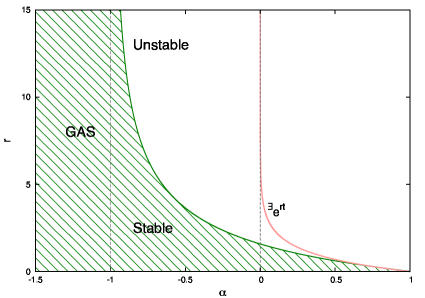
Figure 2.1. Stability region for the positive equilibrium in the $(\alpha,r)$-parameter plane. The shaded region is the stability region given by (2.1) and (2.2). The positive equilibrium is globally stable for $\alpha\leq-1$ and is unstable above the stability boundary. Exponential solutions exist on the denoted curve. Blow-up solutions exist for $\alpha>0$, hence we can observe a region where the positive equilibrium is locally stable yet blow-up solutions also exist.

3. Instability and exponential solutions

A remarkable feature of the logistic equation with positive feedback (1.1) is the possible existence of exponential solutions, despite the equation being nonlinear. As in [7], we find the following.

Proposition 2.

There exists an exponential solution

(3.1) $$x_{c}(t):=ce^{rt},\ t\geq-1$$

of the generalized logistic equation

(3.2) $$\frac{d}{dt}x(t)=rx(t)\left(1+\sum_{i=1}^{k}a_{i}x(t-\tau_{i})\right),$$

if and only if

(3.3) $$\sum_{i=1}^{k}a_{i}e^{-r\tau_{i}}=0.$$

The proof is straightforward, and for (1.1) it means that an exponential solution exists if and only if

(3.4) $$\alpha=e^{-r}$$

holds.

It can be shown that the existence of the exponential solution implies the instability of the positive equilibrium.

Proposition 3.

Let us assume that (3.4) holds. Then the positive equilibrium of (1.1) is unstable.

Proof.

We compare the two conditions (3.4) and (2.3). We set

(3.5) $$\omega=\arccos(\alpha)\text{ for }\alpha\in\left(0,1\right).$$

Note that $\omega\in\left(0,\frac{\pi}{2}\right)$. Using the parameter transformation (3.5) we get

$$\arccos(\alpha)\sqrt{\frac{1-\alpha}{1+\alpha}}=\omega\frac{1-\cos\omega}{\sin\omega}$$

and the condition (3.4) is written as $r=-\ln(\cos\omega)$. Define

$$g_{1}(\omega) :=\omega\frac{1-\cos\omega}{\sin\omega},$$

$$g_{2}(\omega) :=-\ln(\cos\omega)$$

for $\omega\in\left(0,\frac{\pi}{2}\right)$. We claim that

(3.6) $$g_{2}(\omega)>g_{1}(\omega),\ \text{$\omega\in\left(0,\frac{\pi}{2}\right)$}.$$

It is easy to see that $\lim_{\omega\downarrow 0}g_{1}(\omega)=\lim_{\omega\downarrow 0}g_{2}(\omega)=0$. Straightforward calculations show

$$g_{1}^{\prime}(\omega) =\frac{1-\cos\omega}{\sin\omega}\left(1+\frac{\omega}{\sin\omega}\right),$$

$$g_{2}^{\prime}(\omega) =\frac{\sin\omega}{\cos\omega}.$$

Then we see

$$g_{2}^{\prime}(\omega)-g_{1}^{\prime}(\omega) =\frac{1}{\cos\omega\sin\omega}\left\{\sin^{2}\omega-\cos\omega\left(1-\cos\omega\right)\left(1+\frac{\omega}{\sin\omega}\right)\right\}$$

$$=\frac{1-\cos\omega}{\cos\omega\sin\omega}\left\{\left(1+\cos\omega\right)-\cos\omega\left(1+\frac{\omega}{\sin\omega}\right)\right\}$$

$$=\frac{1-\cos\omega}{\cos\omega\sin\omega}\left(1-\omega\frac{\cos\omega}{\sin\omega}\right)$$

$$>0$$

for $\omega\in\left(0,\frac{\pi}{2}\right)$. Thus we get (3.6) and obtain the conclusion. ∎

In Figure 2.1 we visualize the condition (3.4) in $(\alpha,r)$ parameter plane. Figure 2.1 clearly shows that if (3.4) holds, then the positive equilibrium is unstable.

4. A new class of blow-up solutions

We investigate other solutions of (1.1) when (3.4) holds.

Theorem 4.

Let the condition (3.4) hold. Consider a solution with the initial function satisfying

(4.1) $$0<\phi(s)\leq ce^{rs},\ s\in\left[-1,0\right]$$

with

(4.2) $$\phi(0) =c,$$

(4.3) $$\phi(-1) <ce^{-r}$$

for $c>0$. Then one has $x(t)>x_{c}(t)=ce^{rt}$ for $t>0$ and the solution blows up at a finite time.

Proof.

Looking for a contradiction, we assume that $x(t)$ exists on $\left[0,\infty\right)$. Then $x(t)>0,\ t\geq-1$. Define

$$z(t):=\ln\left(\frac{x(t)}{x_{c}(t)}\right)=\ln\left(\frac{x(t)}{ce^{rt}}\right),\ t\geq-1.$$

Let

$$\psi(s):=\ln\left(\frac{\phi(s)}{ce^{rs}}\right),\ s\in[-1,0].$$

Then $z(s)=\psi(s)$ for $s\in\left[-1,0\right]$, and we have

$$0=\psi(0)\geq\psi(s),\quad 0=\psi(0)>\psi(-1),\ s\in\left[-1,0\right]$$

from (4.1), (4.2) and (4.3). Now we obtain the relation

$$\frac{d}{dt}z(t)=\frac{ce^{rt}}{x(t)}\frac{x^{\prime}(t)ce^{rt}-x(t)rce^{rt}}{c^{2}e^{2rt}}=\frac{x^{\prime}(t)}{x(t)}-r,$$

which can be rewritten by using (1.1) and $\alpha=e^{-r}$ as

$$\frac{d}{dt}z(t)=r(e^{-r}x(t)-x(t-1)),$$

and by $x(t)=e^{z(t)}ce^{rt}$ we obtain a nonautonomous differential equation for $z$:

(4.4) $$z^{\prime}(t)=rce^{r\left(t-1\right)}\left(e^{z(t)}-e^{z(t-1)}\right),\ t>0$$

using (3.4). First we show that $z^{\prime}(t)>0$ for any $t\geq 0$. Since

$$\psi(0)=\ln\left(\frac{\phi(0)}{c}\right)=0>\psi(-1)=\ln\left(\frac{\phi(-1)}{ce^{-r}}\right)$$

follows from (4.2) and (4.3), one finds

$$z^{\prime}(0)=rce^{-r}\left(e^{\psi(0)}-e^{\psi(-1)}\right)>0.$$

Assume that there exists $t_{1}>0$ such that $z^{\prime}(t)>0$ for $\ 0\leq t<t_{1}$ and $z^{\prime}(t_{1})=0$ hold. If $t_{1}\in(0,1)$ then, since $t_{1}-1\in\left(-1,0\right)$,

$$z^{\prime}(t_{1})=rce^{r\left(t_{1}-1\right)}\left(e^{z(t_{1})}-e^{z(t_{1}-1)}\right),$$

while

$$z(t_{1})-z(t_{1}-1)=z(t_{1})-z(0)+\psi(0)-\psi(t_{1}-1)>0,$$

thus we obtain a contradiction. If $t_{1}\geq 1$, then

$$z(t_{1})-z(t_{1}-1)=\int_{t_{1}-1}^{t_{1}}z^{\prime}(s)ds>0,$$

which leads a contradiction again. Therefore, we obtain $z^{\prime}(t)>0$ for $t\geq 0$.

We can fix a $T>2$ such that

$$1<\left(1-\alpha\right)re^{-r}ce^{rT}.$$

Since $z(t)$ exists on $\left[0,\infty\right)$ and $z^{\prime}(t)>0$ for $t\geq 0$, $z^{\prime}(t)>0$ for $0\leq t\leq T$. Thus

$$m:=\min_{0\leq t\leq T}z^{\prime}(t)>0.$$

By the intermediate value theorem, for each $0\leq t\leq T$, there exists $\xi(t)\in\left[z(t-1),z(t)\right]$ such that $e^{z(t)}-e^{z(t-1)}=e^{\xi(t)}\left(z(t)-z(t-1)\right)$. Since $\xi(t)\geq z(t-1)>0$, we have

$$z^{\prime}(t) =rce^{r\left(t-1\right)}e^{\xi(t)}\left(z(t)-z(t-1)\right)$$

$$\geq rce^{r\left(t-1\right)}\left(z(t)-z(t-1)\right)$$

$$=rce^{r\left(t-1\right)}\int_{t-1}^{t}z^{\prime}(s)ds.$$

This yields

(4.5) $$z^{\prime}(t)>\int_{t-1}^{t}z^{\prime}(s)ds,\ t\geq T$$

and hence $z^{\prime}(T)>\int_{T-1}^{T}z^{\prime}(s)ds\geq m$. This implies that $z^{\prime}(t)>m$ for $t\geq T$. Otherwise there is a $t_{1}>T>1$ such that $z^{\prime}(t)>m$ for $0<t<t_{1}$ and $z^{\prime}(t_{1})=m$. But from (4.5)

$$z^{\prime}(t_{1})>\int_{t_{1}-1}^{t_{1}}z^{\prime}(s)ds>m,$$

which is a contradiction.

Thus for any $t\geq 1$ we have

$$e^{z(t)}-e^{z(t-1)} =e^{z(t)}\left(1-e^{-\left(z(t)-z(t-1)\right)}\right)$$

$$=e^{z(t)}\left(1-e^{-\int_{t-1}^{t}z^{\prime}(s)ds}\right)$$

$$\geq e^{z(t)}\left(1-e^{-m}\right).$$

Therefore,

$$z^{\prime}(t)\geq rce^{r\left(t-1\right)}e^{z(t)}\left(1-e^{-m}\right),\ t\geq 1,$$

or equivalently

$$z^{\prime}(t)e^{-z(t)}\geq\left(rce^{-r}(1-e^{-m})\right)e^{rt},\ t\geq 1.$$

Integrating both sides of the above equation,

$$\int_{1}^{t}z^{\prime}(s)e^{-z(s)}ds =\left[-e^{-z(s)}\right]_{s=1}^{s=t}=e^{-z(1)}-e^{-z(t)}$$

$$\geq\left(rce^{-r}(1-e^{-m})\right)\int_{1}^{t}e^{rs}ds$$

$$=\left(ce^{-r}(1-e^{-m})\right)(e^{rt}-e^{r}),\ t>1.$$

This yields

$$e^{-z(1)}\geq\left(ce^{-r}(1-e^{-m})\right)(e^{rt}-1)+e^{-z(t)}>\left(ce^{-r}(1-e^{-m})\right)(e^{rt}-1),\ t\geq 1,$$

which is a contradiction. Therefore, $z$ does not exist on $\left[0,\infty\right),$ moreover $z^{\prime}(t)\geq 0,\ t\geq 0$.

Consequently we should have a $T\in\left(0,\infty\right)$ such that $\lim_{t\to T-}z(t)=+\infty$, that is it is a blow-up solution. Corresponding to this blow-up solution, we also have

$$x(t)=ce^{z(t)+rt}\to\infty,\ t\to T^{-},$$

that is $x(t)$ is also a blow-up solution. ∎

Proposition 5.

The following estimate is valid:

$$\frac{1}{r}\ln\left(1+\frac{e^{r}}{c}\right)\leq T,$$

where $T$ is the blow-up time for a blow-up solution $x$ in Theorem 4.

Proof.

We can find the lower bound for the blow-up time $T$ by the standard comparison principle. Consider the following ordinary differential equation

$$y^{\prime}(t)=y(t)r\left(1+e^{-r}y(t)\right)$$

with $y(0)=c=x(0)$. By the comparison theorem, we have $x(t)\leq y(t),\ t\geq 0$. Integrating the equation, we get

$$y(t)=\frac{ce^{rt}}{1+\left(1-e^{rt}\right)e^{-r}c}$$

for sufficiently small $t$. From this expression, we find the finite blow-up time for $y$ and then we obtain the required estimation. ∎

Similar to the proof of Theorem 4, we obtain the following theorem.

Theorem 6.

Let the condition (3.4) hold. Consider a solution with the initial function satisfying

(4.6) $$ce^{rs}\leq\phi(s),\ s\in\left[-1,0\right]$$

with

(4.7) $$\phi(0) =c,$$

(4.8) $$\phi(-1) >ce^{-r}$$

for $c>0$. Then one has $x(t)<x_{c}(t)=ce^{rt}$ for $t>0$, and consequently the solution exists on $[-1,\infty)$.

For the initial functions considered in Theorems 4 and 6, $\frac{x(t)}{x_{c}(t)}$ is a monotone function for $t>0$, thus the order of the solution with respect to the exponential solution, $x_{c}(t)=ce^{rt}$, is preserved. We do not analyze the qualitative behavior of the solution with the initial condition that oscillates about the exponential solution. Numerical simulations suggest that, for many solutions, $\frac{x(t)}{x_{c}(t)}$ eventually becomes a monotone function.

5. Discussion

In this paper we study the logistic equation (1.1). In the stability analysis of delayed logistic equations, negative instantaneous feedback is usually assumed, see [4, 7, 14, 16] and references therein. Only a few stability results are available in the literature for the case of positive instantaneous feedback e.g., [12, 13]. However, the blow-up solutions, which are present due to the positive instantaneous feedback, have not been analyzed in detail, since the publication of the paper [7]. This manuscript has been inspired by the work done in [7], especially, paying attention to the examples and open questions given in Section 5 of the paper [7]. Our primary goal was to clarify and understand a relation between the stability condition of the positive equilibrium and the existence condition for the exponential solution. For the logistic equation (1.1), we show that the existence of the exponential solution implies instability of the positive equilibrium in Proposition 2, see also Fig. 2.1. Since stability analysis becomes extremely hard for the differential equation with multiple delays, the comparison of the existence condition of the exponential solution to the stability condition is not straightforward in general, thus it remains an open problem whether the positive equilibrium of (3.2) is always unstable whenever exists and (3.3) holds.

Finding a global stability condition for (1.1) in the case of $-1<\alpha<0$ is still an open problem. For $\alpha=0$ the global stability problem is known as the famous Wright conjecture [2]. On the other hand, for $0<\alpha<1$, due to the existence of the blow-up solution, it is shown that the stable equilibrium can not attract every solution, thus there is no hope to obtain global stability condition for $0<\alpha<1$. Numerical simulations also suggest that there are many bounded and oscillatory solutions .

In Theorems 4 and 6 we fix the parameters as in (3.4) in Proposition 2 so that the exponential solution exists for the logistic equation (1.1). We consider some solutions that preserve the order with respect to the exponential solution, and show that some blow up, while others exist for all positive time. The qualitative behaviour of the solution with the initial condition that oscillates about the exponential solution is not studied. For such an initial function, careful estimation of the solution seems to be necessary to understand the long term solution behaviour. Numerical simulations suggest that, for many solutions, $\frac{x(t)}{x_{c}(t)}$ eventually becomes a monotone function. The detailed understanding of the evolution of such solutions is also left for future work.

Finally, one might be interested in the equation

$$\frac{d}{dt}y(t)=y(t)r\left(1+\alpha y(t)+y(t-1)\right),$$

which has an opposite sign for the delayed feedback term. For this equation the qualitative dynamics is studied in the literature. The positive equilibrium

$$y^{*}=-\frac{1}{1+\alpha}$$

exists if and only if $\alpha<-1$. According to Theorem 5.6 in Chapter 2 in [11], the positive equilibrium is globally asymptotically stable. When $\alpha\geq-1$ the solutions are unbounded, see again Theorem 5.1 in [7].

Acknowledgement

The first author’s research has been supported by the Hungarian National Research Fund Grant OTKA K120186 and the Széchenyi 2020 project EFOP-3.6.1-16-2016-00015. The second author was supported by JSPS Grant-in-Aid for Young Scientists (B) 16K20976. The third author was supported by Hungarian National Research Fund Grant NKFI FK 124016 and MSCA-IF 748193. The meeting of the authors have been supported by JSPS and NKFI Hungary-Japan bilateral cooperation project.

References

- [1] J.A.D. Appleby, I. Győri, D.W. Reynolds, History-dependent decay rates for a logistic equation with infinite delay. Proc. Roy. Soc. Edinburgh Sect. A 141 (2011), no. 1, 23–44.
- [2] B. Bánhelyi, T. Csendes, T. Krisztin, and A. Neumaier, ,Global attractivity of the zero solution for Wright’s equation, SIAM Journal on Applied Dynamical Systems, 13(2014), 537–563.
- [3] O. Diekmann, S.A. van Gils, S.M.V. Lunel, H.O. Walther, Delay Equations Functional, Complex and Nonlinear Analysis, Springer Verlag (1991).
- [4] T. Faria, E. Liz, Boundedness and asymptotic stability for delayed equations of logistic type. Proc. Roy. Soc. Edinburgh Sect. A 133 (2003), no. 5, 1057–1073.
- [5] E. Liz, G. Röst, Dichotomy results for delay differential equations with negative Schwarzian, Nonlinear Analysis: Real World Applications 11.3 (2010): 1422–1430.
- [6] K. Gopalsamy, Stability and oscillation in delay differential equations of population dynamics. Kluwer Academic Publishers (1992).
- [7] I. Győri, A new approach to the global asymptotic stability problem in a delay Lotka-Volterra differential equation. Mathematical and Computer Modelling 31 6 (2000) pp. 9–28.
- [8] I. Győri, F. Hartung, Fundamental solution and asymptotic stability of linear delay differential equations, Dynamics of Continuous, Discrete and Impulsive Systems, 13:2 (2006) 261–288.
- [9] I. Győri, G. Ladas, Oscillation theory of delay differential equations with applications, Clarendon Press, Oxford (1991).
- [10] X. He, Global stability in nonautonomous Lotka-Volterra systems of “pure-delay type”, Differential and Integral Equations 11.2 (1998) 293–310.
- [11] Y. Kuang, Delay differential equations with applications in population dynamics, Academic Press, San Diego (1993).
- [12] S.M. Lenhart, C.C. Travis, Global stability of a biological model with time delay, Proc. Amer. Math. Sot. 96 (1986) 75–78.
- [13] H. Li, R. Yuan, An affirmative answer to the extended Gopalsamy and Liu’s conjecture on the global asymptotic stability in a population model. Nonlinear Anal. Real World Appl. 11 (2010), no. 5, 3295–3308.
- [14] S. Ruan, Delay differential equations in single species dynamics. In: Delay Differential Equations and Applications, Springer (2006), 477–517.
- [15] G. Stépán, Retarded Dynamical Systems: Stability and Characteristic Function, Wiley, New York, 1989.
- [16] Z. Teng, Permanence and stability in non-autonomous logistic systems with infinite delay. Dyn. Syst. 17 (2002), no. 3, 187–202.