Ionization potential depression and optical spectra in a Debye plasma model

Abstract

We show how optical spectra in dense plasmas are determined by the shift of energy levels as well as the broadening owing to collisions with the plasma particles. In lowest approximation, the interaction with the plasma particles is described by the RPA dielectric function, leading to the Debye shift of the continuum edge. The bound states remain nearly un-shifted, their broadening is calculated in Born approximation. The role of ionization potential depression as well as the Inglis-Teller effect are shown. The model calculations have to be improved going beyond the lowest (RPA) approximation when applying to WDM spectra.

1 Introduction

Optical properties of dense plasmas have become of increasing interest with new experimental facilities exploring warm dense matter (WDM) and materials in the high-energy density regime. Producing plasmas in the region of condensed matter densities and temperatures in the keV region, many-body effects such as the dissolution of bound states owing to the Mott effect and the ionization potential depression (IPD) are within reach. New experiments [1, 2, 3] are devoted to explore these effects which are essential for the ionization degree and the composition of high-energy density matter [4].

Recently, there has been an intense discussion concerning bound state energies which are modified by the surrounding plasma. In particular, experiments can not be described by traditional simple expressions for the IPD [5]. A new quantum statistical approach has been worked out [6] which provides a better agreement with experimental data. The shift of the continuum edge is determined by the single-particle self-energy (SE), and it has been shown that this is related to the dynamical structure factor. In particular, the ion-ion structure factor is essential for the evaluation of the IPD.

Because the experimental observations are mainly related to the optical spectra, this is only an indirect observation of the IPD. Optical spectra are not only determined by the position of the energy levels of the radiator modified by the plasma surrounding, but also by the broadening produced by collisions. The broadening of spectral lines leads to the Inglis-Teller effect (ITE) [7], the peak structures of the optical spectra which are interpreted as spectral lines due to transitions between bound states are washed out. If the overlap between neighbored lines is sufficiently large, they are no longer visible as separate in the optical spectra.

For the interpretation of the disappearance of spectral lines at increasing plasma density there are two accepted but controversial scenarios. Firstly, the IPD becomes sufficiently large so that the bound state shifts into the continuum and disappears. Secondly, the ITE means that separate lines merge due to broadening so that peak structures are washed out. We consider a more fundamental approach where many-particle effects for optical spectra are treated in a systematic way. Within this approach, both IPD and ITE are following from the SE. The real part of the SE describes energy shifts (IPD), whereas its imaginary part is related to line broadening (ITE).

2 Medium modifications

The optical properties in a medium are determined via the absorption coefficient $\alpha(\omega)$, which is related to transversal part of the dielectric function (DF)

$$n(\omega)+ic\,\alpha(\omega)/\omega=\lim_{q\rightarrow 0}\sqrt{{\epsilon}_{\rm tr}({\mathbf{q}},\omega)},$$ (1)

where $c$ is the speed of light in the vacuum and $n(\omega)$ denotes the refraction index. In the long wavelength limit, both the transversal and longitudinal part of the DF $\epsilon({\mathbf{q}},\omega)$ are identical, i.e. ${\epsilon}_{\rm tr}({\mathbf{q}},\omega)={\epsilon}_{\rm long}({\mathbf{q}},\omega)$. In addition, the longitudinal DF ${\epsilon}_{\rm long}({\mathbf{q}},\omega)$ is determined by the polarization function $\Pi({\bf q},\omega)$

$${\epsilon}_{\rm long}({\mathbf{q}},\omega)=1-\frac{e^{2}}{\varepsilon_{0}q^{2}}\Pi({\mathbf{q}},\omega).$$ (2)

The polarization function $\Pi({\mathbf{q}},\omega)$ can be evaluated systematically using thermodynamic Green’s functions and Feynman’s diagrams. Subsequently, a systematic many-particle approach to the optical spectra of dense plasmas is given by the polarization function $\Pi({\bf q},\omega)$ in the long wavelength limit. To obtain the line spectra, a cluster decomposition of the polarization function has to be performed [8, 9],

$$\leavevmode\nobreak\ \Pi({\mathbf{q}},\omega)=\Pi_{1}({\mathbf{q}},\omega)+\Pi_{2}({\mathbf{q}},\omega)+\cdots,$$ (3)

which represent the one-particle $\Pi_{1}({\mathbf{q}},\omega)$ (single-particle states), two-particle contribution $\Pi_{2}({\mathbf{q}},\omega)$ (two-particle states) and so on. Hence we consider the process $X^{Z+}\to X^{(Z+1)+}+e^{-}$ replacing the $Z$-fold charged ion (also including neutral atoms for $Z=0$) by a two-particle problem, the $(Z+1)$ core ion plus the electron.

We consider the interaction with the plasma in the lowest approximation, i.e. the random phase approximation (RPA). The two-particle propagator in $\Pi_{2}$ is modified by a two-particle SE. The corresponding effective equation of motion is denoted as the Bethe-Salpeter equation which reads [6, 8, 10]

$$\Big{[}E(1)+E(2)+\sum_{\bf q}[f(1+{\bf q})+f(2-{\bf q})]V_{12}({\bf q})+\Delta V^{\rm eff}(1,2,{\bf q},z)\Big{]}\!\psi(1,2,z)$$

$$+ \sum_{\bf q}\!\Big{\{}[1\!-\!f(1)\!-\!f(2)]V_{12}({\bf q})+\Delta V^{\rm eff}(1,2,{\bf q},z)\Big{\}}\psi(1+{\bf q},2-{\bf q},z)\ =\ \hbar z\,\psi(1,2,z).$$ (4)

Here, the single particle states $1=\{\hbar{\bf p}_{1},\sigma_{1},c_{1}\}$ are given by momentum, spin and species, respectively, $E(1)=\hbar^{2}{\bf p}_{1}^{2}/(2m_{1})$. In the case considered here $c_{1}$ denotes the electron, charge number $Z_{e}=-1$, and $c_{2}$ the core ion. For the interaction we assume the Coulomb potential $V_{12}({\bf q})=Z_{c_{1}}Z_{c_{2}}e^{2}/(\varepsilon_{0}q^{2})$. $z$ is a complex variable following from the analytical continuation of the functions, defined for the Matsubara frequencies, into the entire $z$ plane. Of interest is the behavior of the functions near the real axis, $z=\omega\pm i\epsilon$.

The in-medium Schrödinger equation (2) describes the influence of the medium by two effects, Pauli blocking and screening. Pauli blocking arises from the fact that states which already are occupied by the medium are blocked. The blocking is described by the Fermi distribution function $f(1)=[\exp(\beta(E(1)-\mu(1))+1]^{-1}$ in Eq. (2), with $\beta=1/(k_{B}T)$ and $\mu(1)$ denoting the chemical potential of species $c_{1}$. Screening of the interaction by the medium is described by the effective interaction

$$\Delta V^{\rm eff}(1,2,{\bf q},z) =-V_{12}({\bf q})\int_{-\infty}^{\infty}\frac{d\omega^{\prime}}{\pi}{\rm Im}\,\varepsilon^{-1}(q,\omega^{\prime}+i0)\,\left[{n}_{\rm{}_{B}}(\omega^{\prime})+1\right]$$

$$\times\left(\frac{\hbar}{\hbar z-\hbar\omega^{\prime}-E(1)-E(2-{\bf q})}+\frac{\hbar}{\hbar z-\hbar\omega^{\prime}-E(1+{\bf q})-E(2)}\right).$$ (5)

Including the effective potential, the effective Hamiltonian in the in-medium Schrödinger equation (2) becomes complex and frequency dependent. This equation can be solved numerically [11], where both, real part and imaginary part of the energy levels of the in-medium two-particle problem, can be calculated. In other words, the energy levels are shifted by the polarization of the medium and are also broadened by collisions with the plasma particles which leads to a finite life time of the energy levels. From Eq. (2), bound states are found at negative energies, whereas a continuum of scattering states is observed at positive energies with negative continuum edges.

The remaining task is to determine the DF $\varepsilon(q,z)$ in the effective potential, i.e. Eq. (2). A standard expression for the DF $\varepsilon(q,z)$ is the RPA DF. In the present work, we will use the RPA DF to calculate the IPD and the spectral lines in plasmas. Within this simplest approximation, we provide an insight to the explanation of the question how the ITE and the IPD can be systematically and consistently described within a unified theory.

2.1 Shift of single particle states

The definition of free states is generally described via $E_{\mathbf{p}}=\hbar^{2}\mathbf{p}^{2}/(2m_{c})$ for the atomic species $c$ with the wavenumber $\mathbf{p}$. In a medium the interaction between particles must be considered. Consequently, the definition of free states has to be modified by taking into account the interaction potential $V(\mathbf{r}\rightarrow\infty)$. Within the framework of Green’s function technique, the shift of the continuum edge is assumed to occur at ${\bf p}_{1}={\bf p}_{2}=0$ in Eq. (2). Consequently, the influence of the surrounding plasmas is described by [6]

$${\Sigma}^{{\rm corr}}_{c}(p,\omega)=\sum_{\mathbf{q}}\Delta V^{\rm eff}(p,-p,{\bf q},\omega)=-\sum_{\mathbf{q}}\int\frac{d\omega^{\prime}}{\pi}V_{cc}(q)\,\frac{\left\{1+{n}_{\rm{}_{B}}(\omega^{\prime})\right\}\,{\rm Im}\,\varepsilon^{-1}(q,\omega^{\prime}+i0)}{\omega-\omega^{\prime}-E_{c,{\bf p}+{\bf q}}/\hbar}.$$ (6)

The shift of the continuum lowering is then given by the real part of this expression (6). Following the theory in Ref. [6], the imaginary part of the inverse DF in Eq. (6) can be expressed via the dynamical structure factors according to the fluctuation-dissipation theorem. Considering only the ionic contribution to the continuum lowering, the shift of the continuum edge is obtained

$${\Delta}^{{\rm ion-ion}}_{c}(0,\omega)-{\cal P}\!\!\int\!\frac{d^{3}{\bf q}}{(2\pi)^{3}}\!\int\!\frac{d\omega^{\prime}}{\pi}\frac{V_{cc}(q)}{\omega-\omega^{\prime}-E_{c,{\bf q}}/\hbar}\frac{\pi Z_{i}e^{2}\,n_{e}}{\hbar\epsilon_{0}\,q^{2}}{S}^{{\rm ZZ}}_{\rm\rm ii}(q,\omega^{\prime}),$$ (7)

where ${S}^{{\rm ZZ}}_{\rm\rm ii}(q,\omega^{\prime})$ is the effective ion structure factor which includes the screening cloud formed by the slowly moving electrons following the ionic motion [6, 12]. In the classical limit $(\hbar\omega=\hbar p^{2}/(2{m}_{\rm ion})=0)$ and plasmon pole approximation, the IPD is determined by the difference between the SE before and that after the ionization of the investigated system, i.e., ${\Delta}^{{\rm ion-ion}}_{\rm{}_{IPD}}={\Delta}^{{\rm ion-ion}}_{i}-({\Delta}^{{\rm ion-ion}}_{e}+{\Delta}^{{\rm ion-ion}}_{i+1})$. Then we have for the IPD

$${\Delta}^{{\rm ion-ion}}_{\rm{}_{IPD}}=-\frac{(Z+1)e^{2}}{2\pi^{2}\epsilon_{0}r_{{}_{\rm WS}}}\cdot\frac{3\Gamma_{i}}{\sqrt{(9\pi/4)^{2/3}+3\Gamma_{i}}}\cdot\int_{0}^{\infty}\frac{dq_{0}}{q_{0}^{2}}{S}^{{\rm ZZ}}_{\rm\rm ii}(q_{0}),$$ (8)

where $q_{0}=q/\left(3\pi^{2}n_{i}\right)^{1/3}$ is the reduced wavenumber. $\Gamma_{i}=Z^{2}e^{2}/(4\pi\epsilon_{0}k_{B}Tr_{{}_{\rm WS}})$ is the ionic coupling parameter with the Wigner-Seitz radius $r_{{}_{\rm WS}}=(4\pi n_{i}/3)^{-1/3}$.

2.2 Shift of two-particle states

To investigate the optical spectra within the quantum statistical approach, we should return to the two-particle problem, which is described by the atomic polarization function $\Pi_{2}$ in Eq. (3). The pressure-broadened line profile is then given by [13, 14]

$${\cal L}(\omega)=\sum_{ii^{\prime}ff^{\prime}}\frac{\omega^{4}}{8\pi^{3}\,c^{3}}\,e^{-\frac{\hbar\omega}{{k}_{\rm B}T}}\,\langle i|\mathbf{r}|f\rangle\langle f^{\prime}|\mathbf{r}|i^{\prime}\rangle\cdot\langle i^{\prime}|\langle f^{\prime}|\,\left[\hbar\omega-\hbar\omega_{if}-\Sigma_{if}(\omega)+i{\Gamma}^{{\rm v}}_{if}\right]^{-1}\,|i\rangle|f\rangle$$ (9)

with the SE for the initial $i$ and final $f$ states

$$\Sigma_{if}(\omega)={\rm Re}\,\left\{\Sigma_{i}(\omega)-\Sigma_{f}(\omega)\right\}+i{\rm Im}\,\left\{\Sigma_{i}(\omega)+\Sigma_{f}(\omega)\right\}$$ (10)

and the vertex correction

$${\Gamma}^{{\rm v}}_{if}=-\int\frac{d^{3}\mathbf{p}}{(2\pi)^{3}}\int\frac{d^{3}\mathbf{q}}{(2\pi)^{3}}{f}_{\rm e}(E_{\mathbf{p}})\,V^{2}(q)\,M^{0}_{ii}({\mathbf{q}})M^{0}_{ff}({-\mathbf{q}})\,\delta\left(\frac{\hbar^{2}\mathbf{p\cdot q}}{{m}_{\rm e}}\right)$$ (11)

where the unperturbed transition matrix elements are given by [14]

$$M^{0}_{n\alpha}({\mathbf{q}})=i\left\{Z\delta_{n\alpha}-\int d^{3}\mathbf{r}\ \psi_{n}^{*}(\mathbf{r})\,e^{i\mathbf{q\cdot r}}\,\psi_{\alpha}(\mathbf{r})\right\}.$$ (12)

Evidently, the shift of transition energy is given by the difference of real parts of the SE for the initial $i$ and final $f$ states, whereas the broadening of spectral lines is determined by the imaginary parts of the SE for the initial $i$ and final $f$ states as well as the vertex correction ${\Gamma}^{{\rm v}}_{if}$. Because of different dynamical time scales of ions and electrons, the electronic contribution is usually calculated in the impact approximation and the ionic contribution is described within the quasi-static approximation [13, 15].

Introducing the microfield ansatz [13], the total SE $\Sigma_{n}(\omega,F)$ can be approximately decomposed into a frequency-independent ionic part determined by the microfield strength $F$ and an only frequency-dependent electronic part. In this work, we deal with the problem in a different way by treating the plasma electrons and ions at the same level, i.e. directly via the DF. The RPA DF for the non-degenerate case reads [8, 16]

$${\epsilon}_{\rm RPA}({\mathbf{q}},\omega) =1+\frac{K}{2Q^{3}}\bigg{\{}\sqrt{2}\left[D(x_{1}^{+})-D(x_{1}^{-})\right]+\sqrt{2/\gamma}\left[D(x_{2}^{+})-D(x_{2}^{-})\right]$$

$$- i\Big{\{}\sqrt{\pi/2}\left[e^{-(x_{1}^{+})^{2}}-e^{-(x_{1}^{-})^{2}}\right]+\sqrt{\pi/(2\gamma)}\left[e^{-(x_{2}^{+})^{2}}-e^{-(x_{2}^{-})^{2}}\right]\Big{\}}\bigg{\}}$$ (13)

with the abbreviations

$$Q=\frac{\hbar q}{\left({m}_{\rm e}\,{k}_{\rm B}T\right)^{1/2}}\,,\qquad K=\frac{(1+z^{2})\hbar^{2}{n}_{\rm e}e^{2}}{{m}_{\rm e}\,\varepsilon_{0}\,({k}_{\rm B}T)^{2}}\,,\qquad\gamma=\frac{{m}_{\rm e}}{{m}_{\rm ion}}\,$$

$$x_{1}^{\pm}=\sqrt{\frac{1}{2}}\,\left[\frac{\omega}{q}\left(\frac{{m}_{\rm e}}{{k}_{\rm B}T}\right)\pm\frac{Q}{2}\right]\,,\qquad x_{2}^{\pm}=\sqrt{\frac{1}{2\gamma}}\,\left[\frac{\omega}{q}\left(\frac{{m}_{\rm e}}{{k}_{\rm B}T}\right)\pm\gamma\frac{Q}{2}\right],$$ (14)

where $D(x)=\exp\left(-x^{2}\right)\int_{0}^{x}dt\,\exp\left(-t^{2}\right)$ is the Dawson integral. Inserting this expression into the Eq. (6), an expression for the IPD can be obtained, which is the Debye shift for the IPD in the low density case and is equivalent to the expression (8). Instead of starting from Eq. (2), we calculate the SE of bound two-particle states with the following expression [9, 13]

$$\leavevmode\nobreak\ {\Sigma}_{n}(\omega)=\int\frac{d^{3}{\mathbf{q}}}{(2\pi\hbar)^{3}}V(q)\,\sum_{\alpha}\left|{M^{0}_{n\alpha}({\mathbf{q}})}\right|^{2}\int_{-\infty}^{\infty}\frac{d\omega}{\pi}\frac{\left[1+{n}_{\rm{}_{B}}(\omega)\right]\cdot{\rm Im}\,{\epsilon}_{\rm RPA}^{-1}({\mathbf{q}},\omega+i0)}{E_{n}-E_{\alpha}-\left(\hbar\omega+i0\right)},$$ (15)

which is the SE in dynamically screened Born approximation with the RPA DF. Accounting for the thermal motion of the plasma ions, which results in the Doppler broadening, the full line profile is given by a convolution [15]

$${I}^{{\rm total}}(\Delta\omega)=\frac{c}{\omega_{0}}\sqrt{\frac{{m}_{\rm ion}}{2\pi{k}_{\rm B}T}}\int_{-\infty}^{\infty}d\Delta\omega^{\prime}\cdot{I}^{{\rm pr}}(\Delta\omega^{\prime})\cdot\exp\left\{-\frac{{m}_{\rm ion}c^{2}}{2{k}_{\rm B}T}\,\left(\frac{\Delta\omega-\Delta\omega^{\prime}}{\omega_{0}+\Delta\omega^{\prime}}\right)^{2}\right\}.$$ (16)

3 Results and discussion

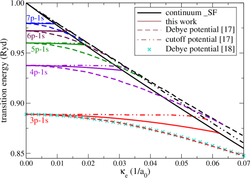
Figure 1: Transition energy for the Lyman series $\hbar\omega=E_{n\mathrm{p}}-{E}_{\rm 1s}$ and the threshold energy for the bound-free transition $\hbar{\omega}_{\rm th}=V(\infty)-{E}_{\rm 1s}$ with respect to the inverse Debye length of electrons ${\kappa}_{\rm e}$. The solid lines represent the results of this work. The dashed lines and the dotted-dashed lines describe the numerical results of the Schrödinger equation with a Debye potential [17, 18] and a cutoff potential [17], respectively. The cross points are also calculated with Debye potential [18].

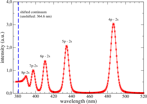
Figure 2: Optical spectra of a plasma at the electron density ${n}_{\rm e}=2.1\cdot 10^{17}\,\mathrm{cm}^{-3}$ and temperature ${T}_{\rm e}=1.02$ eV calculated within RPA (15). Gaussian broadening with FWHM of 0.002 Ryd is considered in the calculation. Both ITE and IPD are systematically calculated from the quantum statistical approach. A continuum background [14] is considered.

The interaction of a radiating particles with the plasma environment results in both shift and broadening of the eigenlevels of a two-particle state. At first, we concentrate on the shifts of both the bound states and the free states. In the present work, we calculate the IPD and the shift of bound states via Eq. (8) and Eq. (15), respectively. Comparison of our results for the transition energies and bound-free threshold energies and the results predicted by other theoretical approaches is shown is Fig. 1.

The positions of emission line centers are determined by the transition energies. One of the commonly used theoretical approaches is to solve the Schrödinger equation with a pseudo-potential [17, 18] for eigenenergies and the corresponding wave functions. Numerical solutions have been obtained using the Debye potential [17, 18] or the cutoff potential [17, 19] as the pseudo-potential. From Fig. 1, it is seen that the line center positions derived from the cutoff potentials are almost unchanged in comparison to the pure Coulomb case. In contrast, the Debye potential predicts a strong modification for the transition energy, in particular for relatively high densities (${\kappa}_{\rm e}=\sqrt{{n}_{\rm e}e^{2}/(\varepsilon_{0}{k}_{\rm B}T)}\geq 0.02/a_{0}$). However, this result is in strong contradiction to the experimental measurements, where the positions of line centers are only slightly shifted [19]. In the Debye model, the shifts do not separately depend on density and temperature but only on the screening parameter ${\kappa}_{\rm e}$.

The optical spectra of the Balmer series calculated within RPA combined with a continuum background due to Bremsstrahlung are displayed in Fig. 2. For the given plasma conditions (${n}_{\rm e}=2.1\cdot 10^{17}\,\mathrm{cm}^{-3}$, ${T}_{\rm e}=1.02$ eV), the IPD value is about $0.138$ eV, which means that the energy levels appear only up to $n=9$ and the Balmer limit is shifted from $364.6$ nm to $380.8$ nm. Another feature of the predicted line shape (i.e. ITE) is the formation of quasi-continuum states, i.e. the band structure, starting from the energy level $n=6$. Moreover, the transition peak from $\mathrm{9p}\rightarrow\mathrm{2s}$ is washed out due to the broadening. In summary, to calculate the spectra in the whole wavelength range, the first step is to determine the highest existing quantum state from the IPD theory. The second step is to calculate the line shape up to the highest energy level predicted by the IPD theory. Actually, the optical spectra of Balmer series under these conditions were experimentally measured by Goto et al. [20], where the disappearance of the transition peaks is observed already starting from a lower principal quantum number $n=6$. The reason for this disagreement arises from the fact that the ionic contribution to the broadening is excessively underestimated by RPA. Comparing the experimentally measured line broadening of H_α line with the RPA result, it is shown that the RPA result is only $25\%$ of the experimental value.

The line merging due to the broadening does not have a simple relation to the shift of the continuum edge. Generally, both effects have to be considered carefully and comprehensively for correctly reproducing the experimental spectra. For weakly coupled and non-degenerate plasmas, the line merging occurs at lower principal quantum numbers in comparison to the IPD effect as shown in Fig. 2 and measured in laser produced plasmas [1, 21]. Recently, the optical spectra in highly charged aluminum plasmas are observed, where the continuum lowering is so large that the lines disappear before they are subject to broadening sufficient to merge them [1]. Therefore, it is of relevance to develop an accurate spectral line theory using the systematic quantum statistical approach, since spectroscopic methods are the most reliable tool to analyze density and temperature conditions.

4 Conclusions, further improvements

We have shown that both effects, IPD and ITE, have to be considered to explain the disappearance of spectral lines. The synthetic spectra and the transition energies are systematically described using a consistent quantum statistical approach within the simplest RPA. The Debye results for both IPD and optical transitions are obtained. Of course, the Debye model is very simple and the ionic contributions are strongly underestimated. For the hydrogen plasmas, the ion contribution is more important. The RPA is not satisfied and has to be improved. The underestimation might be rendered by using the ionic structure factor to calculate the line broadening and shift like in the case for the IPD when going beyond the RPA [6]. Additionally, the electron contribution can be improved by introducing the T matrix describing strong collisions. Furthermore, photon re-absorption plays an important role for the transport of radiation in a plasma, which has a strong influence on the transitions from the low quantum numbers [14]. This has to be taken into account in calculating the line shapes. For higher levels, the transition rates may be better described via semi-classical description, for example using wave-packet states for the electrons [22].

In the context of new experimental facilities exploring warm dense matter [1, 2, 3, 21], strongly coupled and nearly degenerate Coulomb systems can be produced. A detailed description of the spectrum emitted from such systems in equilibrium and non-equilibrium conditions is still a challenging problem. As shown in this work, the quantum statistical approach based on thermodynamic Green’s function technique provides a possibility to understand the many-body systems under such extreme conditions.

References

- [1] D. J. Hoarty et al., Phys. Rev. Lett. 110, 265003 (2013).
- [2] O. Ciricosta et al., Phys. Rev. Lett. 109, 065002 (2012); Nat. Commun. 7, 11713 (2016).
- [3] D. Kraus et al., Phys. Rev. E 94, 011202( R) (2016).
- [4] H.-K. Chung et al., High Energ. Dens. Phys. 1, 3 (2005).
- [5] G. Ecker and W. Kröll, Phys. Fluids 6, 62 (1963); J. C. Stewart and K. D. Pyatt, Jr., Astrophys. J. 144, 1203 (1966).
- [6] C. Lin et al.., Phys. Rev. E 96, 013202 (2017).
- [7] D. R. Inglis and E. Teller, ApJ 90, 439, (1939).
- [8] W.-D. Kraeft et al., Quantum Statistics of Charged Particle Systems (Akademie-Verlag Berlin, 1986).
- [9] G. Röpke and R. Der, phys. stat. sol. (b) 92, 501 (1979).
- [10] R. Zimmermann et al., phys. stat. sol. (b) 88, K59 (1978); phys. stat. sol. (b) 90, 175 (1978).
- [11] J. Seidel, S. Arndt, and W.-D. Kraeft, Phys. Rev. E 52, 5387 (1995).
- [12] G. Gregori, A. Ravasio, A. Höll, S. H. Glenzer and S. J. Rose, High Energy Density Phys. 3, 99 (2007).
- [13] S. Günter, L. Hitzschke, and G. Röpke, Phys. Rev. A 44, 6834 (1991).
- [14] B. Omar, A. Wierling, and G. Röpke, Contrib. Plasmas Phys. 51, 22 (2011).
- [15] H. Griem, Plasma Spectroscopy, ( McGraw-Hill 1964).
- [16] R. Redmer, Physics Reports 282, 35 (1997).
- [17] F. E. Höhne and R. Zimmermann, J. Phys. B: At. Mol. Phys. 15, 25551 (1985).
- [18] Y. Y. Qi et al., Physics of Plasmas 16, 023502 (2009).
- [19] R. Radtke and K. Günther, Contrib. Plasmas Phys. 26, 143 (1986); Contrib. Plasmas Phys. 26, 151 (1986).
- [20] M Goto et al., Plasma Phys. Control. Fusion 49, 1163 (2007).
- [21] M. Nantel et al., Phys. Rev. Lett. 80, 4442 (1998).
- [22] C. Lin et al., Phys. Rev. E 93, 042711 (2016).