On the Theory of Light Propagation in Crystalline Dielectrics

Abstract

A synoptic view on the long-established theory of light propagation in crystalline dielectrics is presented, where charges, tightly bound to atoms (molecules, ions) interact with the microscopic local electromagnetic field. Applying the Helmholtz-Hodge decomposition to the current density in Maxwell’s equations, two decoupled sets of equations result determining separately the divergence-free (transversal) and curl-free (longitudinal) parts of the electromagnetic field, thus facilitating the restatement of Maxwell’s equations as equivalent field-integral equations. Employing a suitably chosen basis system of Bloch functions we present for dielectric crystals an exact solution to the inhomogenous field-integral equations determining the local electromagnetic field that polarizes individual atoms or ionic subunits in reaction to an external electromagnetic wave. From the solvability condition of the associated homogenous integral equation then the propagating modes and the photonic bandstructure $\omega_{n}\left(\mathbf{q}\right)$ for various crystalline symmetries $\Lambda$ are found solving a small sized $3M\times 3M$ matrix eigenvalue problem, with $M$ denoting the number of polarizable atoms (ions) in the unit cell. Identifying the macroscopic electric field inside the sample with the spatially low-pass filtered microscopic local electric field, the dielectric $3\times 3$-tensor $\varepsilon_{\Lambda}\left(\mathbf{q},\omega\right)$ of crystal optics emerges, relating the accordingly low-pass filtered microscopic polarization field to the macroscopic electric field, solely with the individual microscopic polarizabilities $\alpha\left(\mathbf{R},\omega\right)$ of atoms (molecules, ions) at a site $\mathbf{R}$ and the crystalline symmetry as input into the theory. Decomposing the microscopic local electric field into longitudinal and transversal parts, an effective wave equation determining the radiative part of the macroscopic field in terms of the transverse dielectric tensor $\varepsilon_{ab}^{\left(T\right)}\left(\mathbf{q},\omega\right)$ is deduced from the exact solution to the field-integral equations. The Taylor expansion $\varepsilon_{ab}^{\left(T\right)}\left(\mathbf{q},\omega\right)=\varepsilon_{ab}^{\left(T\right)}\left(\omega\right)+i\sum_{c}\gamma_{abc}\left(\omega\right)q_{c}+\sum_{c,d}\alpha_{abcd}\left(\omega\right)q_{c}q_{d}+...$ around $\mathbf{q}=\mathbf{0}$ provides then insight into various optical phenomena connected to retardation and non-locality of the dielectric tensor, in full agreement with the phenomenological reasoning of Agranovich and Ginzburg in “Crystal Optics with Spatial Dispersion, and Excitons” (Springer Berlin Heidelberg, 1984): the eigenvalues of the tensor $\varepsilon_{ab}^{\left(T\right)}\left(\omega\right)$ describing chromatic dispersion of the index of refraction and birefringence, the first order term $\gamma_{abc}\left(\omega\right)$ specifying rotary power (natural optical activity), the second order term $\alpha_{abcd}\left(\omega\right)$ shaping the effects of a spatial-dispersion-induced birefringence, a critical parameter for the design of lenses made from $CaF_{2}$ and $BaF_{2}$ for optical lithography systems in the ultraviolet. In the static limit an exact expression for $\varepsilon_{\varLambda}$ is deduced, that conforms with general thermodynamic stability criteria and reduces for cubic symmetry to the Clausius-Mossotti relation. Considering various dielectric crystals comprising atoms with known polarizabilities from the literature, in all cases the calculated indices of refraction, the rotary power and the spatial-dispersion-induced birefringence coincide well with the experimental data, thus illustrating the utility of the theory. For ionic crystals, exemplarily for $CsI$ and $RbCl$, a satisfactory agreement between theory and the measured chromatic dispersion of the index of refraction is shown over a wide frequency interval, ranging from ultraviolet to far infra-red, accomplishing this with an appreciably smaller number of adjustable parameters compared to the well known Sellmeier fit.

I Introduction

When optical signals traverse a transparent dielectric, for example a fused quartz (silica) prism, the light travels at different speed depending on frequency $f=\frac{\omega}{2\pi}$ , so that the shape of a wave packet, say composed of mixed frequencies $\left|f-f_{c}\right|\leq\frac{\varDelta f_{c}}{2}$ around a carrier frequency $f_{c}$ in a frequency interval of width $\varDelta f_{c}$, tends to spread out. This is the well known chromatic dispersion effect resulting from the frequency dependence of the refractive index $n=n\left(\omega\right)$. Microscopic considerations based on first principles reveal, that the frequency dependence of the refractive index $n\left(\omega\right)$ is directly connected to the retarded response of the polarizable constituents of matter, the latter distinguishing themselves as atoms, molecules or ions. The chromatic dispersion effect is further supplemented by the effects of crystalline anisotropy and also by the effects of spatial dispersion brought about by the non local dependence of this response, that is a charge at point $\mathbf{r}$ recollects the action exerted on it at another position $\mathbf{r}^{\prime}$ (L.V.Keldysh2012, ; Maksimov2012, ).

Both fundamental features of the electromagnetic response, retardation and non locality, can be described jointly by a dielectric (tensor) function $\varepsilon_{\Lambda}\left(\mathbf{q},\omega\right)$ depending on (circular) frequency $\omega$ and on wave vector $\mathbf{q}$. While the dependence of the dielectric function on $\omega$ explains the chromatic dispersion effect, and its anisotropy for $\mathbf{q}=\mathbf{0}$ describes birefringence, the dependence on wave vector $\mathbf{q}$ is directly connected to phenomena like natural optical activity and spatial dispersion induced birefringence. Furthermore, under the influence of a static magnetic induction field $\mathbf{B}^{\left(0\right)}$, respectively a static electric field $\mathbf{E}^{\left(0\right)}$, the additional dependence of the dielectric function on those static fields gives rise to many other magneto-optic and electro-optic phenomena, for instance the Faraday effect, the Pockels effect and also the Kerr effect (Agranovich1984, ).

When electromagnetic waves propagate inside a dielectric material, the microscopic local electric field convoyed by those waves exerts a small supplemental force onto charge carriers inside the atoms (ions, molecules) comprising that material, pulling apart inside each atom the positively charged nucleus and the negatively charged bound electrons by a (small) shift in opposite direction. Of course the position of the total mass of a charge neutral atom, considering valence electrons and nucleus together, remains then unchanged. Since the atomic nucleus is certainly much heavier than the bound electrons, the resulting shift of the barycenter of the bound electrons by far surpasses the associated tiny shift of the position of the atomic nucleus. This is the effect of induced electronic polarization.

A fully microscopic theory of the optical properties of a material certainly requires to consider the positive charged atomic nuclei and the electrons, taking into account the laws of quantum statistical physics and low energy quantum electrodynamics, for example (L.V.Keldysh2012, ; H.Bilz1984, ). In the ensuing discussion we shall accept a phenomenological (semiclassical) picture of the matter light interaction based on the fundamental fact, that matter is stable, i.e. the energy of an atom located at a site $\mathbf{R}$ is, in the absence of external fields, a minimum against any (small) displacement of its bound electrons. Accordingly, in reaction to the presence of a (weak) local time dependent electric field $\mathbf{E}\left(\mathbf{R},t\right)$ the electrons bound to an atom redistribute themselves, so that considered from outside, an atom comprising a number $Z$ of electrons, acquires an induced electric dipole moment. This is the basic idea of the phenomenological classical model of atomic polarizability due to Lorentz, who described the induced dipole moment of electrons, tied to a heavy (immobile) nucleus by a harmonic spring, solving a harmonic oscillator problem with that local electric field acting as a drive. Incidentally, the Lorentz model predicts a frequency dependent Fourier amplitude

of the induced electronic dipole moment of an atom at site $\mathbf{R}$ that coincides with a full quantum mechanical calculation, see supplemental material (Supplementary, ):

$$\tilde{d}_{a}\left(\mathbf{R},\omega\right) = \sum_{a^{\prime}}\alpha_{a,a^{\prime}}\left(\mathbf{R},\omega\right)\tilde{E}_{a^{\prime}}\left(\mathbf{R},\omega\right)$$ (1)

$$a,a^{\prime} \in \left\{x,y,z\right\}$$

Here $\alpha_{a,a^{\prime}}\left(\mathbf{R},\omega\right)$ denotes the atom-individual electric polarizability given by

$$\alpha_{a,a^{\prime}}\left(\mathbf{R},\omega\right)=\frac{\left|e\right|^{2}}{m}\sum_{\nu\neq 0}\frac{f_{a,a^{\prime}}\left(\nu;\mathbf{R}\right)}{\omega_{\nu}^{2}\left(\mathbf{R}\right)-\left(\omega+\frac{i}{2\tau_{\nu}\left(\mathbf{R}\right)}\right)^{2}}\>,$$ (2)

the summation index $\nu$ running here over all eigenstates $\left|\Phi_{\nu}\left(\mathbf{R}\right)\right\rangle$ of the multi-electron configration of that atom except the groundstate $\left|\Phi_{0}\left(\mathbf{R}\right)\right\rangle$. Indeed, this expression looks like it was derived from an ensemble of (classical) harmonic oscillators with resonance frequencies $\omega_{\nu}\left(\mathbf{R}\right)$, each oscillator being driven by the local electric field with a factor of proportionality $f_{a,a^{\prime}}\left(\nu;\mathbf{R}\right)>0$, the so called oscillator strength. However, the physical meaning of the oscillator strength is only revealed by quantum mechanics. With $\hat{d}_{a}=-\left|e\right|\sum_{n=1}^{Z}\hat{r}_{a}^{\left(n\right)}$ denoting the dipole operator of the count $Z$ of electrons tied to an atom at position $\mathbf{R}$, then according to quantum mechanics

$$f_{a,a^{\prime}}\left(\nu;\mathbf{R}\right) = \frac{1}{\left|e\right|^{2}}\frac{2m}{\hbar}\omega_{\nu}\left(\mathbf{R}\right)\left\langle\Phi_{0}\left(\mathbf{R}\right)|\hat{d}_{a}|\Phi_{\nu}\left(\mathbf{R}\right)\right\rangle\left\langle\Phi_{\nu}\left(\mathbf{R}\right)|\hat{d}_{a^{\prime}}|\Phi_{0}\left(\mathbf{R}\right)\right\rangle\>,$$ (3)

explaining why the oscillator strength is a measure for how much a bound electron contributes to the electric polarizability of an atom, say under a transition from the multi-electron ground state $\left|\Phi_{0}\left(\mathbf{R}\right)\right\rangle$ of the atom Hamiltonian with eigenvalue $\hbar\Omega_{0}\left(\mathbf{R}\right)$ to an excited multi-electron eigenstate $\left|\Phi_{\nu}\left(\mathbf{R}\right)\right\rangle$ with eigenvalue $\hbar\Omega_{\nu}\left(\mathbf{R}\right)$. The differences $\omega_{\nu}\left(\mathbf{R}\right)\equiv\Omega_{\nu}\left(\mathbf{R}\right)-\Omega_{0}\left(\mathbf{R}\right)$ in (2) are the optical transition frequencies, the life-time parameter $\tau_{\nu}\left(\mathbf{R}\right)>0$ describes spontaneous emission as reasoned by quantum electrodynamics and thus being always present if the atom was excited to an eigenstate state $\nu\neq 0$. Expanded details how the result (2) can be derived within first order time dependent perturbation theory in response to a weak time dependent electric field, including a discussion of the $f$-sum rule, see supplemental material (Supplementary, ).

De facto, the spectrum of atoms with $Z>1$ cannot be calculated ab initio with sufficient precision, the exact taking into account of electronic correlations being (alas) an unsolved problem. In what follows we therefore conceive the optical transition frequencies $\omega_{\nu}\left(\mathbf{R}^{\left(j\right)}\right)$, the life-time parameter $\tau_{\nu}\left(\mathbf{R}^{\left(j\right)}\right)$ and the oscillator strengths $f_{a,a^{\prime}}\left(\nu,\mathbf{R}^{\left(j\right)}\right)$ of each atom species positioned at a site $\mathbf{R}^{\left(j\right)}=\mathbf{R}+\bm{\eta}^{\left(j\right)}$, with $\mathbf{R}\in\Lambda$ a lattice vector and $\bm{\eta}^{\left(j\right)}$ indicating a position of an atom (ion, molecule) inside a unit cell $C_{\Lambda}$ of the crystal $\Lambda$, as fitting parameters, so that the optical properties as calculated from the dielectric tensor $\varepsilon_{\Lambda}\left(\mathbf{q},\omega\right)$ of the crystal coincide with experiment. How this objective can be accomplished, and in particular how $\varepsilon_{\Lambda}\left(\mathbf{q},\omega\right)$ depends on the individual atom polarizabilities $\alpha_{a,a^{\prime}}\left(\bm{\eta}^{\left(j\right)},\omega\right)$, and thus via (2) on the atom individual multi-electron spectrum, we shall elaborate in what follows.

A time dependent external electromagnetic signal $\mathbf{E}_{ext}\left(\mathbf{r},t\right)$ incident upon a material probe polarizes the atoms inside, and for weak amplitude of the incident field the induced polarization at the atom sites $\mathbf{R}$ will then be proportional to that amplitude. However the microscopic local electric field $\mathbf{E}\left(\mathbf{r},t\right)$ polarizing an atom (ion, molecule) positioned at site $\mathbf{R}$ is not known a priory, because all atoms in the sample will get polarized and hence all act back with a (retarded) reaction in response to the primary external field $\mathbf{E}_{ext}\left(\mathbf{r},t\right)$. Then everywhere inside (and outside) of the probe there holds

$$\mathbf{E}\left(\mathbf{r},t\right)=\mathbf{E}_{ext}\left(\mathbf{r},t\right)+\mathbf{E}_{ind}\left(\mathbf{r},t\right),$$ (4)

the secondary induced electric field $\mathbf{E}_{ind}\left(\mathbf{r},t\right)$ being a superposition of the individually radiated and retarded electric fields emitted by all the atoms inside the sample, that have been polarized in turn by that field $\mathbf{E}\left(\mathbf{r},t\right)$. With a suitable model of the polarizability of individual atoms thus an integral equation determining the microscopic local electric field $\mathbf{E}\left(\mathbf{r},t\right)$ emerges.

So far, everything said is well known from the original (early) literature (Ewald1916, ; Ewald1916a, ; Ewald1917, ; Ewald1938, ; Laue1931, ) and from highly cited textbooks on crystal optics, for example (Born1999, ; Fluegge2013, ; Agranovich1984, ; Laue1960, ). For a concise summary of the pioneering works on crystal optics of Ewald and v. Laue (and later authors) see (Authier2012, ). Nevertheless, we believe the approach we present in what follows truely discerns from traditional presentations of the subject. For example, nowhere do we make use of the Ewald-Oseen extinction theorem to recover the correct index of refraction $n$ of a material, it being customary practice in the so called rigorous theory of dispersion (Born1999, ; Fluegge2013, ) to consider the wave incident from free space to be propagated with vacuum light velocity $c$ and the signal induced in the sample to be propagated with velocity $c/n$, the Lorentz-Lorenz formula connecting the index of refraction $n$ with the polarizability of individual atoms thus emerging as a solvability condition for the field-integral equation stated (implicitely) in (4).

Outline

In Sec. II we first establish on the basis of the fundamental Maxwell equations an exact integral equation for the microscopic local electric field $\mathbf{E}\left(\mathbf{r},t\right)$ in (4) with an explicit formula for the integral kernel that derives directly from the atom polarizability (2). Posing boundary conditions for the components of the electromagnetic field at the boundary of a material probe is then redundant. Moreover, the frequency dependence of longitudinal and transversal parts of the electromagnetic field are treated consistently, thus making everywhere in our calculations the correct static limit $\omega\rightarrow 0$ accessible.

In Sec. III we solve the field-integral equation for crystalline dielectric materials exactly making use of a set of non-standard Bloch functions, not constructed from plane waves but designed from eigenfunctions of the position operator, representing a complete orthonormal system of eigenfunctions of the translation operator $T_{\mathbf{R}}$ under a shift by a lattice vector $\mathbf{R}\in\Lambda$. Accordingly, instead of expanding the kernel of the field-integral equation in the well known basis of plane waves $e^{i\left(\mathbf{q}+\mathbf{G}\right)\mathbf{r}}$, thus requiring to handle for each wave vector $\mathbf{q}$ in the Brillouin zone $C_{\Lambda^{-1}}$ of a lattice $\Lambda$ then (infinite) matrices labelled by reciprocal lattice vectors $\mathbf{G},\mathbf{G}^{\prime}\in\Lambda^{-1}$, our choice of eigenfunctions of the translation operator $T_{\mathbf{R}}$ sidesteps the inversion (and truncation) of such large matrices, thus easing notably the determination of the photonic bandstructure of a crystal. Also we show, if the incident electromagnetic wave was purely transversal, yet the microscopic local electric field features both, a transversal and a longitudinal component, see Fig.(4), the strength of the longitudinal component being strongly dependent on the density of polarizable atoms (ions, molecules) in the crystal.

Thereafter we present, exemplifying our calculation method, results for the photonic bandstructure of diamond ($M=2$), that have been calculated previously with other (computationally more time-consuming) methods. Our findings for the photonic bandstructures for various monoatomic Bravais lattices ($M=1$) we present and discuss in the supplemental material (Supplementary, ). In comparison to well known (phenomenological) work on photonic bandstructures (Leung1990, ; Zhang1990, ), within which the (macroscopic) Maxwell’s equations in a superlattice are solved assuming a spatially repetetive varying index of refraction, it turns out that in our approach based on the field-integral equations the need to eliminate unphysical “longitudinal” modes doesn’t arise.

In section IV we introduce the notion of a macroscopic electric field $\mathcal{\bm{E}}\left(\mathbf{r},t\right)$ inside a material, conceiving it with regard to spatial variations as a low pass filtered signal, with the solution to the field-integral equation (33) as input. Relating the macroscopic polarization to that macroscopic electric field, thereafter the macroscopic dielectric $3\times 3-$tensor $\varepsilon_{\Lambda}\left(\mathbf{q},\omega\right)$ of a crystalline dielectric material emerges, with chromatic and spatial dispersion fully taken into account. The exact expression for $\varepsilon_{\Lambda}\left(\mathbf{q},\omega\right)$ thus obtained is solely dependent on the symmetry of the lattice $\varLambda$ under consideration and on the polarizability $\alpha\left(\mathbf{R}^{\left(j\right)},\omega\right)$ of individual atoms (ions, molecules) positioned at their equilibrium sites $\mathbf{R}^{\left(j\right)}$ in the crystal. We also confirm, exemplarily for the ionic crystal $CsI$, that our formula for the dielectric tensor with regard to its frequency dependence indeed obeys to the Lyddane-Sachs-Teller relation. With a view to the key role of locality claimed by macroscopic electrodynamics (Liu2009, ) we caution the reader not to discard the $\mathbf{q}$-dependence of the dielectric tensor $\varepsilon_{\Lambda}\left(\mathbf{q},\omega\right)$. As emphasized by Ginzburg and Agranovich (Agranovich1984, ), a rich variety of optical effects, including rotary power and spatial dispersion induced birefringence, manifestly proof the importance of the non local nature of the dielectric response.

We next derive directly from the microscopic field-integral equations a set of differential equations that determine the spatial variation of the transversal and longitudinal parts of the macroscopic electric field $\mathcal{\bm{E}}\left(\mathbf{r},t\right)$, without prior knowledge of the microscopic local field $\mathbf{E}\left(\mathbf{r},t\right)$.

If the external field was purely transversal, this set of coupled differential equations reduces to a wave equation determining the radiative part of the macroscopic field. In this way the parts of the dielectric tensor $\varepsilon_{\Lambda}\left(\mathbf{q},\omega\right)$ are indentified that determine the transversal dielectric tensor $\varepsilon^{\left(T\right)}\left(\mathbf{q},\omega\right)$ comprising the optical properties of a dielectric crystal. Assuming spatial dispersion is a weak effect, which assumption applies for many transparent media, the Taylor expansion of $\varepsilon_{ab}^{\left(T\right)}\left(\mathbf{q},\omega\right)$ around $\mathbf{q}=\mathbf{0}$ then provides (yet in an implicit manner) access to various optical phenomena featuring the propagation of light in dielectric crystals (Agranovich1984, ), for instance chromatic dispersion and birefringence, rotary power (natural optical activity) and also the (weak) effects of a spatial-dispersion-induced birefringence, the latter being a critical problem for the design of lens elements made from crystalline materials like $CaF_{2}$ and $BaF_{2}$ widely used in optical lithograpy systems in the ultraviolet (Burnett2002, ; Serebryakov2003, ). Further we summarize in section IV, see Table 1, Fig.10 and also Fig.11, to what large extend our theory of the dielectric tensor for crystalline dielectrics agrees with measurements over a wide range of optical frequencies for a series of well known crystalline materials, including for example Bi₁₂TiO₂₀ and also Bi₁₂SiO₂₀, both crystals featuring a large number of basis atoms ($M=66$) in the unit cell, thus demonstrating the utility of our approach.

If on the other hand the external field was purely longitudinal, the differential equations derived from the field-integral equations reduce to a Poisson type equation for a scalar potential function determining the macroscopic electric field, thus identifying the parts of the dielectric tensor $\varepsilon_{\Lambda}\left(\mathbf{q},\omega\right)$ featuring electric-field screening, like in electrostatics. Also we deduce an exact analytic formula for the static dielectric tensor $\varepsilon_{\Lambda}$, that conforms with general thermodynamic stability criteria (Kirzhnitz2012, ) and applies for all $14$ monoatomic Bravais lattices ($M=1$). For the special case of cubic symmetry the long-known Clausius-Mossotti relation is recovered.

II The Field-Integral Equations

Consider a fixed inertial frame, with a polarizable dielectric material at rest occupying a volume $\Omega$ in that frame. Without loss of generality let the microscopic charge density inside $\Omega$ be given the representation

$$\rho\left(\mathbf{r},t\right)=\bm{-\nabla}\cdot\mathbf{P}\left(\mathbf{r},t\right),$$ (5)

with $\mathbf{P}\left(\mathbf{r},t\right)$ denoting the vector field of electric polarization (L.V.Keldysh2012, ). We find it then convenient to decompose the associated microscopic current density

$$\mathbf{j}\left(\mathbf{r},t\right)=\partial_{t}\mathbf{P}\left(\mathbf{r},t\right)$$ (6)

flowing inside $\Omega$ into longitudinal and transversal parts. To serve this purpose we introduce integral kernels

$$\Pi_{aa^{\prime}}^{\left(L\right)}\left(\mathbf{r}-\mathbf{r}^{\prime}\right) = \lim_{\kappa\rightarrow\infty}\int\frac{d^{3}q}{\left(2\pi\right)^{3}}e^{i\mathbf{q}\cdot\mathbf{\left(\mathbf{r}-\mathbf{r}^{\prime}\right)}}\bar{\Pi}_{aa^{\prime}}^{\left(L\right)}\left(\mathbf{q}\right)\frac{1}{1+\frac{\left|\mathbf{q}\right|^{2}}{\kappa^{2}}}$$ (7)

$$\Pi_{aa^{\prime}}^{\left(T\right)}\left(\mathbf{r}-\mathbf{r}^{\prime}\right) = \lim_{\kappa\rightarrow\infty}\int\frac{d^{3}q}{\left(2\pi\right)^{3}}e^{i\mathbf{q}\cdot\mathbf{\left(\mathbf{r}-\mathbf{r}^{\prime}\right)}}\bar{\Pi}_{aa^{\prime}}^{\left(T\right)}\left(\mathbf{q}\right)\frac{1}{1+\frac{\left|\mathbf{q}\right|^{2}}{\kappa^{2}}}$$

with labels $a,a^{\prime},a^{\prime\prime}\in\left\{x,y,z\right\}$ specifying Cartesian components, and

$$\bar{\Pi}_{aa^{\prime}}^{\left(L\right)}\left(\mathbf{q}\right) = \frac{q_{a}q_{a^{\prime}}}{\left|\mathbf{q}\right|^{2}}\;,$$ (8)

$$\bar{\Pi}_{aa^{\prime}}^{\left(T\right)}\left(\mathbf{q}\right) = \delta_{a,a^{\prime}}-\frac{q_{a}q_{a^{\prime}}}{\left|\mathbf{q}\right|^{2}}\;.$$

Denoting the convolution of two kernels $A_{aa^{\prime}}\left(\mathbf{r},\mathbf{r}^{\prime}\right)$ and $B_{aa^{\prime}}\left(\mathbf{r},\mathbf{r}^{\prime}\right)$ with the symbol

$$\left[A\circ B\right]_{aa^{\prime}}\left(\mathbf{r},\mathbf{r}^{\prime}\right)=\int_{\Omega_{P}}d^{3}r^{\prime\prime}\sum_{a^{\prime\prime}}A_{aa^{\prime\prime}}\left(\mathbf{r},\mathbf{r}^{\prime\prime}\right)B_{a^{\prime\prime}a^{\prime}}\left(\mathbf{r}^{\prime\prime},\mathbf{r}^{\prime}\right),$$ (9)

and writing for the kernel representing unity

$$\left[I\right]_{aa^{\prime}}\left(\mathbf{r},\mathbf{r}^{\prime}\right)=\delta_{aa^{\prime}}\delta^{\left(3\right)}\left(\mathbf{r}-\mathbf{r}^{\prime}\right),$$ (10)

then the validity of all the relations distinctive for projection operators are readily confirmed:

$$\Pi^{\left(L\right)}+\Pi^{\left(T\right)} = I$$ (11)

$$\Pi^{\left(L\right)}\circ\Pi^{\left(L\right)} = \Pi^{\left(L\right)}$$

$$\Pi^{\left(T\right)}\circ\Pi^{\left(T\right)} = \Pi^{\left(T\right)}$$

$$\Pi^{\left(T\right)}\circ\Pi^{\left(L\right)} =\>0\>= \Pi^{\left(L\right)}\circ\Pi^{\left(T\right)}$$

In position space, for $\left|\mathbf{\mathbf{r}}\right|\neq 0$, the kernel of the longitudinal and the transverse projection operator both correspond to a dipole field, see (ClaudeCohen-Tannoudji1989, ) for a concise derivation:

$$\Pi_{aa^{\prime}}^{\left(T\right)}\left(\mathbf{r}\right) = \frac{2}{3}\delta_{a,a^{\prime}}\delta^{\left(3\right)}\left(\mathbf{\mathbf{r}}\right)+\Theta\left(\left|\mathbf{\mathbf{r}}\right|-0^{+}\right)\nabla_{a}\nabla_{a^{\prime}}\left(\frac{1}{4\pi\left|\mathbf{r}\right|}\right)$$ (12)

$$\Pi_{aa^{\prime}}^{\left(L\right)}\left(\mathbf{r}\right) = \frac{1}{3}\delta_{a,a^{\prime}}\delta^{\left(3\right)}\left(\mathbf{\mathbf{r}}\right)-\Theta\left(\left|\mathbf{\mathbf{r}}\right|-0^{+}\right)\nabla_{a}\nabla_{a^{\prime}}\left(\frac{1}{4\pi\left|\mathbf{r}\right|}\right)$$

It follows from what has been said that the longitudinal part (L) , respectively the transversal part (T) of the current distribution $j_{a}\left(\mathbf{r},t\right)$ conforms with the convolution integrals

$$j_{a}^{(L,T)}(\mathbf{r},t)=\int d^{3}r^{\prime}\sum_{a^{\prime}}\Pi_{aa^{\prime}}^{\left(L,T\right)}\left(\mathbf{r}-\mathbf{r}^{\prime}\right)j_{a^{\prime}}(\mathbf{r}^{\prime},t).$$ (13)

It should be underlined, this link between the original vector field $\mathbf{j}(\mathbf{r},t)$ and the associated longitudinal (transversal) part $\mathbf{j}^{\left(L,T\right)}(\mathbf{r},t)$ is non local. There holds by construction

$$\mathbf{j}(\mathbf{r},t) = \mathbf{j}^{(L)}(\mathbf{r},t)+\mathbf{j}^{(T)}(\mathbf{r},t)$$ (14)

$$\bm{\nabla}\mathbf{\cdot j}^{(T)}(\mathbf{r},t) = 0$$

$$\mathbf{\bm{\nabla}}\wedge\mathbf{j}^{(L)}(\mathbf{r},t) = \mathbf{0}.$$

According to the Helmholtz-Hodge theorem such a decomposition of a vector field $\mathbf{j}\left(\mathbf{r},t\right)$ is unique. A recent thourough discussion and compilation of the literature on the subject can be found in (Bhatia2013, ).

Because Maxwell’s equations are linear, particular monochromatic solutions

$$\mathbf{E}^{(L,T)}\left(\mathbf{r},t\right) = \mathbf{\tilde{E}}^{(L,T)}\left(\mathbf{r},\omega\right)e^{-i\omega t}$$ (15)

$$\mathbf{B}\left(\mathbf{r},t\right) = \mathbf{\tilde{B}}\left(\mathbf{r},\omega\right)e^{-i\omega t},$$

with Fourier amplitudes $\mathbf{\tilde{E}}^{(L,T)}\left(\mathbf{r},\omega\right)$ and $\mathbf{\tilde{B}}\left(\mathbf{r},\omega\right)$, can be superposed to construct any wanted time dependence. Applying next the projection operators $\Pi_{aa^{\prime}}^{\left(L,T\right)}$ to the in time Fourier transformed Maxwell equations, there emerge two groups of decoupled equations in the space-frequency domain for the respective Fourier amplitudes. The first group relates to the components $\tilde{E}_{a}^{\left(L\right)}(\mathbf{r},\omega)$ of the Fourier amplitudes of the longitudinal electric field,

$$\bm{\nabla}\mathbf{\cdot\tilde{E}}^{(L)}(\mathbf{r},\omega) = \frac{1}{\varepsilon_{0}}\tilde{\varrho}\left(\mathbf{r},\omega\right)$$ (16)

$$-i\omega\varepsilon_{0}\tilde{E}_{a}^{\left(L\right)}(\mathbf{r},\omega)+\tilde{j}_{a}^{(L)}(\mathbf{r},\omega) = 0\;,$$

the second group involves the Cartesian components of the Fourier amplitudes of the transversal electromagnetic field, which obey to the following six inhomogenous scalar Helmholtz equations, the respective source terms being provided by the Fourier amplitudes of the transversal current density, with $c=\frac{1}{\sqrt{\varepsilon_{0}\mu_{0}}}$ the speed of light in free space:

$$\left(-\nabla^{2}-\frac{\omega^{2}}{c^{2}}\right)\tilde{E}_{a}^{(T)}\left(\mathbf{r},\omega\right) = \mu_{0}i\omega\tilde{j}_{a}^{(T)}\left(\mathbf{r},\omega\right)$$ (17)

$$\left(-\nabla^{2}-\frac{\omega^{2}}{c^{2}}\right)\tilde{B}_{a}\left(\mathbf{r},\omega\right) = \mu_{0}\left[\mathbf{\bm{\nabla}}\wedge\tilde{\mathbf{j}}(\mathbf{r},\omega)\right]_{a}$$

We are interested to solve (16) and (17) considering now a geometry consisting of two disjoint material bodies at rest, see Fig.1, i.e. $\Omega=\Omega_{S}\cup\Omega_{P}$ and $\Omega_{S}\cap\Omega_{P}=\emptyset$.

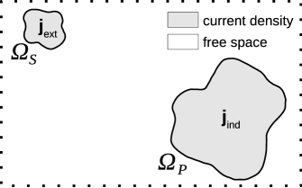
Figure 1: Schematic illustration of a source domain $\Omega_{\text{S}}$ and a probe volume $\Omega_{\text{P}}$ indicating non vanishing current densities inside.

Let us refer to the body $\Omega_{S}$ as the source, and to the body $\Omega_{P}$ as the probe. Accordingly, we split the current density $\tilde{j}_{a}\left(\mathbf{r},\omega\right)$ into an externally controlled partial current $\tilde{j}_{ext,a}\left(\mathbf{r},\omega\right)$ flowing solely inside $\Omega_{S}$, and into an induced partial current $\tilde{j}_{ind,a}\left(\mathbf{r},\omega\right)$ flowing solely inside the probe $\Omega_{P}$:

$$\tilde{j}_{a}\left(\mathbf{r},\omega\right) = \begin{cases}\tilde{j}_{ext,a}\left(\mathbf{r},\omega\right)&\textrm{for}\>\mathbf{r}\in\Omega_{S}\\ \tilde{j}_{ind,a}\left(\mathbf{r},\omega\right)&\textrm{for}\>\mathbf{r}\in\Omega_{P}\\ 0&\textrm{for}\>\mathbf{r}\notin\Omega_{S}\cup\Omega_{P}\end{cases}$$ (18)

If the source $\Omega_{S}$ was a cavity producing a laser beam, and if the surface of the probe $\Omega_{P}$ would be reflecting (parts) of the radiation incident back into that cavity, certainly there would exist a backaction from the probe to the source, leading then to the existence of an induced partial current flowing also inside the source region $\Omega_{S}$. We preclude here and in the following any such backaction effects. Provided transfer of charge between $\Omega_{S}$ and $\Omega_{P}$ is prohibited, there holds charge conservation separately (!) inside $\Omega_{S}$ and inside $\Omega_{P}$. Consequently, inside the domain $\Omega_{S}$ there holds

$$i\omega\tilde{\rho}_{ext}(\mathbf{r},\omega)=\bm{\nabla}\cdot\mathbf{\tilde{j}}_{ext}(\mathbf{r},\omega).$$ (19)

Of course $\tilde{\rho}_{ext}(\mathbf{r},\omega)\equiv 0$ and $\tilde{j}_{ext,a}\left(\mathbf{r},\omega\right)\equiv 0$ for $\mathbf{r}\notin\Omega_{S}$.

It follows from (16) that the longitudinal electric field $\tilde{E}_{a}^{\left(L\right)}(\mathbf{r},\omega)$ is already determined by the longitudinal part of the current distribution (18), a seemingly simple result. Indeed from (16) and (18) then

$$\tilde{E}_{a}^{(L)}\left(\mathbf{r},\omega\right)=\tilde{E}_{ext,a}^{(L)}\left(\mathbf{r},\omega\right)+\frac{1}{\epsilon_{0}}\frac{1}{i\omega}\tilde{j}_{ind,a}^{\left(L\right)}\left(\mathbf{r},\omega\right),$$ (20)

where the external longitudinal field

$$\tilde{E}_{ext,a}^{(L)}\left(\mathbf{r},\omega\right)=\frac{1}{\epsilon_{0}}\frac{1}{i\omega}\tilde{j}_{ext,a}^{\left(L\right)}\left(\mathbf{r},\omega\right)\equiv-\frac{\partial}{\partial r_{a}}\tilde{\phi}_{ext}(\mathbf{r},\omega)$$ (21)

is derived from a scalar potential

$$\tilde{\phi}_{ext}(\mathbf{r},\omega)=\int_{\Omega_{S}}d^{3}r^{\prime}\frac{\tilde{\rho}_{ext}(\mathbf{r}^{\prime},\omega)}{4\pi\varepsilon_{0}\left|\mathbf{r}-\mathbf{r}^{\prime}\right|},$$ (22)

like in electrostatics. Even though $\tilde{j}_{ext,a}(\mathbf{r},\omega)$ was restricted to be non vanishing solely inside the source domain $\Omega_{S}$, its longitudinally projected part $\tilde{j}_{ext,a}^{\left(L\right)}\left(\mathbf{r},\omega\right)$ also exists outside of $\Omega_{S}$, the non locality of that projection thus becoming manifest.

The electromagnetic fields radiated by the transversal current density $\tilde{j}_{a}^{(T)}\left(\mathbf{r},\omega\right)$ in (17) can be readily determined introducing the retarded Green’s function

$$\tilde{g}\left(\mathbf{r}-\mathbf{r}^{\prime},\omega\right) = \frac{\exp\left(i\frac{\omega}{c}\left|\mathbf{r}-\mathbf{r}^{\prime}\right|\right)}{4\pi\left|\mathbf{r}-\mathbf{r}^{\prime}\right|}$$ (23)

$$\mathtt{Im}\left(\omega\right) \rightarrow 0^{+},$$

with $\tilde{g}\left(\mathbf{r}-\mathbf{r}^{\prime},\omega\right)$ the solution of the three-dimensional inhomogeneous scalar Helmholtz equation in free space $\mathbb{R}^{3}$ with a point source (of strength unity) at position $\mathbf{r}^{\prime}$:

$$\left(-\nabla^{2}-\frac{\omega^{2}}{c^{2}}\right)\tilde{g}\left(\mathbf{r}-\mathbf{r}^{\prime},\omega\right)=\delta^{\left(3\right)}\left(\mathbf{r}-\mathbf{r}^{\prime}\right)$$ (24)

As the distance $\left|\mathbf{r}-\mathbf{r}^{\prime}\right|$ to the source position at $\mathbf{r}^{\prime}$ increases then $\tilde{g}\left(\mathbf{r}-\mathbf{r}^{\prime},\omega\right)$ behaves like an outgoing spherical wave.

Based on Green’s identity applied to the domain $\Omega=\Omega_{S}\cup\Omega_{P}$, and again applied to the complementary domain $\mathbb{R}^{3}\setminus\Omega$, there follow directly from (17) and (24) for all points $\mathbf{r}\notin\Omega_{S}$ the integral representations

$$\tilde{E}_{a}^{(T)}\left(\mathbf{r},\omega\right)=\tilde{E}_{ext,a}^{(T)}\left(\mathbf{r},\omega\right)+i\omega\mu_{0}\int d^{3}r^{\prime}\tilde{g}\left(\mathbf{r}-\mathbf{r}^{\prime},\omega\right)\tilde{j}_{ind,a}^{(T)}\left(\mathbf{r}^{\prime},\omega\right)$$ (25)

and

$$\tilde{B}_{a}\left(\mathbf{r},\omega\right)=\tilde{B}_{ext,a}\left(\mathbf{r},\omega\right)+\mu_{0}\int d^{3}r^{\prime}\tilde{g}\left(\mathbf{r}-\mathbf{r}^{\prime},\omega\right)\left[\mathbf{\bm{\nabla}^{\prime}}\wedge\tilde{\mathbf{j}}_{ind}(\mathbf{r}^{\prime},\omega)\right]_{a}.$$ (26)

For details of the derivation of (25) and (26), see supplemental material (Supplementary, ).

According to (6) the Fourier amplitude of the induced current density flowing inside the probe volume $\Omega_{P}$ is directly proportional to the Fourier amplitude of the microscopic electric polarization:

$$\tilde{j}_{ind,a}\left(\mathbf{r},\omega\right)=-i\omega\tilde{P}_{a}\left(\mathbf{r},\omega\right)$$ (27)

Combining now the respective longitudinal and transverse parts by adding the integral representations (20) and (25) there follows

$$\tilde{E}_{a}\left(\mathbf{r},\omega\right)=\tilde{E}_{ext,a}\left(\mathbf{r},\omega\right)+\frac{1}{\epsilon_{0}}\int d^{3}r^{\prime}\sum_{a^{\prime}}\mathcal{\tilde{G}}_{aa^{\prime}}(\mathbf{r}-\mathbf{r}^{\prime},\omega)\tilde{P}_{a^{\prime}}\left(\mathbf{r}^{\prime},\omega\right),$$ (28)

with

$$\mathcal{\tilde{G}}_{aa^{\prime}}(\mathbf{r}-\mathbf{r}^{\prime},\omega) = \frac{\omega^{2}}{c^{2}}\int d^{3}s\>\tilde{g}\left(\mathbf{r}-\mathbf{s},\omega\right)\Pi_{aa^{\prime}}^{\left(T\right)}\left(\mathbf{s}-\mathbf{r}^{\prime}\right)-\Pi_{aa^{\prime}}^{\left(L\right)}\left(\mathbf{r}-\mathbf{r}^{\prime}\right)$$

$$= \lim_{\kappa\rightarrow\infty}\int\frac{d^{3}q}{\left(2\pi\right)^{3}}\frac{e^{i\mathbf{q}\cdot\left(\mathbf{r}-\mathbf{r}^{\prime}\right)}}{1+\frac{\left|\mathbf{q}\right|^{2}}{\kappa^{2}}}\left[\frac{\omega^{2}}{c^{2}}\frac{\delta_{a,a^{\prime}}-\frac{q_{a}q_{a^{\prime}}}{\left|\mathbf{q}\right|^{2}}}{\left|\mathbf{q}\right|^{2}-\frac{\omega^{2}}{c^{2}}-i0^{+}}-\frac{q_{a}q_{a^{\prime}}}{\left|\mathbf{q}\right|^{2}}\right]$$

denoting the electromagnetic kernel. The Fourier transformed kernel $\mathcal{\tilde{G}}_{aa^{\prime}}(\mathbf{r},\omega)$ in the wave vector domain we denote as

$$\mathcal{\bar{G}}_{aa^{\prime}}(\mathbf{q},\omega) = \int d^{3}re^{-i\mathbf{q}\cdot\mathbf{r}}\mathcal{\tilde{G}}_{aa^{\prime}}(\mathbf{r},\omega)$$

$$= \frac{\omega^{2}}{c^{2}}\frac{\delta_{a,a^{\prime}}-\frac{q_{a}q_{a^{\prime}}}{\left|\mathbf{q}\right|^{2}}}{\left|\mathbf{q}\right|^{2}-\frac{\omega^{2}}{c^{2}}-i0^{+}}-\frac{q_{a}q_{a^{\prime}}}{\left|\mathbf{q}\right|^{2}}$$

$$= \frac{\frac{\omega^{2}}{c^{2}}\delta_{a,a^{\prime}}-q_{a}q_{a^{\prime}}}{\left|\mathbf{q}\right|^{2}-\frac{\omega^{2}}{c^{2}}-i0^{+}}\>.$$

Assuming a small amplitude of the perturbing external field $\tilde{E}_{ext,a}\left(\mathbf{r},\omega\right)$ there results inside the probe at a position $\mathbf{r}\in\Omega_{P}$ the (total) microscopic polarization

$$\tilde{P}_{a}\left(\mathbf{r},\omega\right)=\varepsilon_{0}\int_{\Omega_{P}}d^{3}r^{\prime}\sum_{a^{\prime}}\tilde{\chi}_{ext,aa^{\prime}}\left(\mathbf{r},\mathbf{r}^{\prime},\omega\right)\tilde{E}_{ext,a^{\prime}}\left(\mathbf{r}^{\prime},\omega\right)\>.$$ (31)

Within a fully microscopic approach the response kernel $\tilde{\chi}_{ext,aa^{\prime}}\left(\mathbf{r},\mathbf{r}^{\prime},\omega\right)$ is calculated from Kubo’s formula in reaction to the presence of the external field $\tilde{E}_{ext,a^{\prime}}\left(\mathbf{r}^{\prime},\omega\right).$ However, what we are really interested in here, is not the response kernel $\tilde{\chi}_{ext,aa^{\prime}}\left(\mathbf{r},\mathbf{r}^{\prime},\omega\right)$ connecting the polarization $\tilde{P}_{a}\left(\mathbf{r},\omega\right)$ inside the probe with the external field $\tilde{E}_{ext,a^{\prime}}\left(\mathbf{r}^{\prime},\omega\right)$, but the dielectric susceptibility kernel $\tilde{\chi}_{aa^{\prime}}\left(\mathbf{r},\mathbf{r}^{\prime},\omega\right)$ connecting $\tilde{P}_{a}\left(\mathbf{r},\omega\right)$ with the microscopic local electric field $\tilde{E}_{a^{\prime}}\left(\mathbf{r}^{\prime},\omega\right)$ that acts on each atom (ion, molecule):

$$\tilde{P}_{a}\left(\mathbf{r},\omega\right)=\varepsilon_{0}\int_{\Omega_{P}}d^{3}r^{\prime}\sum_{a^{\prime}}\tilde{\chi}_{aa^{\prime}}\left(\mathbf{r},\mathbf{r}^{\prime},\omega\right)\tilde{E}_{a^{\prime}}\left(\mathbf{r}^{\prime},\omega\right)$$ (32)

As emphasized by Keldysh (L.V.Keldysh2012, ), there is no need to consider dielectric and magnetic susceptibilities separately, the latter being already incorporated in the non locality of the dielectric kernel.

The fundamental field-integral equation determining the microscopic local electric field is then given by an inhomogenous integral equation comprising the dielectric kernel $\tilde{\chi}$:

$$\tilde{E}_{a}\left(\mathbf{r},\omega\right)=\tilde{E}_{ext,a}\left(\mathbf{r},\omega\right)+\int_{\Omega_{P}}d^{3}r^{\prime}\sum_{a^{\prime}}\left[\mathcal{\tilde{G}}\circ\tilde{\chi}\right]_{aa^{\prime}}\left(\mathbf{r},\mathbf{r}^{\prime},\omega\right)\tilde{E}_{a^{\prime}}\left(\mathbf{r}^{\prime},\omega\right)$$ (33)

The link between the dielectric susceptibility kernel $\tilde{\chi}$ and the response kernel $\tilde{\chi}_{ext}$ is readily identified (L.V.Keldysh2012, ), combining (31) with (32):

$$\tilde{\chi}=\tilde{\chi}_{ext}\circ\left[I+\mathcal{\tilde{G}}\circ\tilde{\chi}_{ext}\right]^{-1}=\left[I+\tilde{\chi}_{ext}\circ\mathcal{\tilde{G}}\right]^{-1}\circ\tilde{\chi}_{ext}$$ (34)

For a more detailed explanation, see supplemental material (Supplementary, ). So, if $\tilde{\chi}_{ext}$ was known, say from a full microscopic calculation with Kubo’s formula, then $\tilde{\chi}$ follows from (34). In case the probe volume $\Omega_{P}$ was of finite size, solving the integral equation (34) for the microscopic dielectric susceptibility kernel $\tilde{\chi}$ poses a formidable (numerical) problem, the non-locality radius of $\tilde{\chi}_{ext}$ being substantially enhanced up to the macroscopic scale by the presence of a boundary (L.V.Keldysh2012, ). In the next section III we circumvent this problem and introduce a phenomenological model for $\tilde{\chi}$ that proves a posteriori to be appropriate to describe in detail the propagation of light in dielectric crystals.

III Microscopic Local Electric Field in Crystalline Dielectrics

Crystalline order assumes each equilibrium position of atoms (ions, molecules) inside a material corresponds to a site vector $\mathbf{R}^{\left(j\right)}=\mathbf{R}+\bm{\eta}^{\left(j\right)}$, where $\mathbf{R}$ denotes a lattice vector in a Bravais lattice $\Lambda$, and $\bm{\eta}^{\left(j\right)}$ with $j\in\left\{1,2,...,M\right\}$ is a set of position vectors indicating equilibrium positions of the atoms (molecules, ions) inside the unit cell $C_{\Lambda}$. The entire probe volume $\Omega_{P}$ can be thought of to be filled translating a number $\left|\Lambda_{P}\right|$ of Wigner-Seitz unit cells $C_{\Lambda}$ by lattice vectors $\mathbf{R}\in\Lambda$. This subset of all such Bravais lattice vectors $\mathbf{R}\in\Lambda$ we denote as $\Lambda_{P}\subset\Lambda$. Under the action of the external electric field $\tilde{E}_{ext,a^{\prime}}\left(\mathbf{r}^{\prime},\omega\right)$ each atom (ion, molecule) gets polarized proportional to the local electric field $\tilde{E}_{a}\left(\mathbf{R}^{\left(j\right)},\omega\right)$ acting at position $\mathbf{R}^{\left(j\right)}$ of that atom. Then a simple phenomenological model for the microscopic dielectric susceptibility kernel in crystalline insulators emerges assembling first all individual atom contributions located at positions $\bm{\eta}^{\left(j\right)}$ inside the unit cell positioned around the origin $\mathbf{R}=\mathbf{0}$, and then sum over all such cells filling the probe volume $\Omega_{P}$ of the crystal lattice $\Lambda$ under consideration:

$$\tilde{\chi}_{aa^{\prime}}\left(\mathbf{r},\mathbf{r}^{\prime},\omega\right) = \frac{1}{\varepsilon_{0}}\sum_{\mathbf{R}\in\Lambda_{P}}\>\sum_{1\leq j,j^{\prime}\leq M}\alpha_{aa^{\prime}}\left(\bm{\eta}^{\left(j\right)},\bm{\eta}^{\left(j^{\prime}\right)},\omega\right)\delta^{\left(3\right)}\left(\mathbf{r}-\mathbf{R}-\mathbf{\bm{\eta}}^{\left(j\right)}\right)\delta^{\left(3\right)}\left(\mathbf{r}^{\prime}-\mathbf{R}-\bm{\eta}^{\left(j^{\prime}\right)}\right)$$ (35)

$$\alpha_{aa^{\prime}}\left(\bm{\eta}^{\left(j\right)},\bm{\eta}^{\left(j^{\prime}\right)},\omega\right) = \delta_{j,j^{\prime}}\alpha_{aa^{\prime}}^{\left(I\right)}\left(\bm{\eta}^{\left(j\right)},\omega\right)+\left(1-\delta_{j,j^{\prime}}\right)\alpha_{aa^{\prime}}^{\left(II\right)}\left(\bm{\eta}^{\left(j\right)},\bm{\eta}^{\left(j^{\prime}\right)},\omega\right)$$ (36)

Essentially, this susceptibility kernel describes a lattice periodic arrangement of point dipoles (Laue1931, ; Ewald1938, ; Laue1960, ). The diagonal terms $j=j^{\prime}$ refer to the afore mentioned effects of induced electronic polarization of single atoms (ions, molecules) at the positions $\bm{\eta}^{\left(j\right)}$ inside the unit cell $C_{\Lambda}$ around the lattice vector $\mathbf{R}=\mathbf{0}$. Based on the functional form of the frequency dependence of the individual microscopic polarizability (2) of a single atom (ion, molecule), in actual fact being equivalent to a Lorentz-oscillator model, we write now a simple phenomenological ansatz with fitting parameters $\alpha_{0}^{\left(j\right)}$and $\omega_{0}^{\left(j\right)}$(and possibly also including a small life-time parameter $\tau^{\left(j\right)}=1/\gamma^{\left(j\right)}>0$ representing spontaneous emission, see supplemental material (Supplementary, )):

$$\alpha_{aa^{\prime}}^{\left(I\right)}\left(\bm{\eta}^{\left(j\right)},\omega\right)=\delta_{a,a^{\prime}}\frac{\alpha_{0}^{\left(j\right)}}{1-\left[\frac{\omega+\frac{i}{2}\gamma^{\left(j\right)}}{\omega_{0}^{\left(j\right)}}\right]^{2}}$$ (37)

If $\omega\ll\omega_{0}^{\left(j\right)}$ the atom polarizability is well approximated by its static value $\alpha_{0}^{\left(j\right)}$. For most frequencies, except if $\omega$ approaches a transition frequency $\omega_{0}^{\left(j\right)}$ near to an absorption band, we may assume $\gamma^{\left(j\right)}\rightarrow 0^{+}$.

In case there are two or more basis atoms in the Wigner-Seitz cell qualitatively new effects need to be considered. Off diagonal terms $j\neq j^{\prime}$ exist for $M\geq 2$ and designate mutual influences of atoms (ions, molecules) positioned at different sites $\bm{\eta}^{\left(j\right)}$ and $\bm{\eta}^{\left(j^{\prime}\right)}$ inside the unit cell. On one hand, in reaction to the presence of a propagating electromagnetic wave the overlap integral(s) determining the sharing of electron pairs between neighbouring atoms undergo (slight) changes. On the other hand, in crystals like $NaCl$, $CsI$, $RbCl$ etc., the formation of ions needs to be taken into account. Besides the effect of induced electronic polarization of single atoms (ions), attributed to a shift of the barycenter of the electrons bound to individual atoms (ions) under the action of the local field on-site $\mathbf{R}^{\left(j\right)}$, an additional shift of the position of the positive ions relative to the position of the negative ions concurs, thus leading to ionic displacement polarizability. This effect is typically noticeable in the electromagnetic response to radiation with frequency $\omega$ of order of characteristic lattice vibration frequencies $\omega_{ph}$, de facto being mainly of concern for radiation in the infrared.

Conceiving also the off-diagonal polarizabilities $j\neq j^{\prime}$ not as input from microscopic theory, but in the phenomenological guise of a Lorentz-oscillator model for oppositely charged ion pairs (Ashcroft1981, ),

$$\alpha_{aa^{\prime}}^{\left(II\right)}\left(\bm{\eta}^{\left(j\right)},\bm{\eta}^{\left(j^{\prime}\right)},\omega\right)=\delta_{a,a^{\prime}}\frac{\alpha_{0}^{\left(j,j^{\prime}\right)}}{1-\left[\frac{\omega+\frac{i}{2}\gamma^{\left(j,j^{\prime}\right)}}{\omega_{0}^{\left(j,j^{\prime}\right)}}\right]^{2}}\>,$$ (38)

with fitting parameters $\alpha_{0}^{\left(j,j^{\prime}\right)}$, $\omega_{0}^{\left(j,j^{\prime}\right)}$ and small damping $\gamma^{\left(j,j^{\prime}\right)}$, we find the well known chromatic dispersion of the index of refraction $n\left(\omega\right)$ is nicely reproduced by our theory of the dielectric tensor $\varepsilon_{\Lambda}\left(\mathbf{q},\omega\right)$ for a variety of dielectric crystals, see Table 1 in section IV. While the electronic polarizabilities (37) of single atoms are often well approximated by their static value, the ionic displacement polarizabilities (38) have a characteristic dependence on frequency in the infrared. Note, that we refrain adding the contributions of the electronic polarizabilities of single atoms to the contributions of the ionic displacement polarizabilities, there being no justification for this (Ashcroft1981, ).

For example, in the case of $CsI$ with $M=2$ ions in the unit cell, our phenomenological approach in (35) brings into altogether $6$ parameters. These are the two transition frequencies $\omega_{0}^{\left(1\right)}$, $\omega_{0}^{\left(2\right)}$ in the optical regime to model the induced electronic polarization of the two ions together with two values $\alpha_{0}^{\left(1\right)}$, $\alpha_{0}^{\left(2\right)}$ for the individual static polarizabilities of the respective ions, and a third resonance frequency $\omega_{0}^{\left(1,2\right)}$ with associated value $\alpha_{0}^{\left(1,2\right)}$shaping the strength of the ionic displacement polarizabilty, that frequency $\omega_{0}^{\left(1,2\right)}$ being characteristic of lattice vibrational frequencies $\omega_{ph}$. Such a distinction is justifiable if the time scale for electronic polarization of individual ions is much faster than the time scale for the lattice vibrations: $\omega_{ph}\simeq\omega_{0}^{\left(1,2\right)}\ll\min\left(\omega_{0}^{\left(1\right)},\omega_{0}^{\left(2\right)}\right)$. With the model (35) we then successfully reproduced experimental data for the chromatic dispersion of the refraction index $n\left(\omega\right)$, exemplarily for $CsI$ and $RbCl$, over a wide frequency interval ranging from ultraviolet to infrared, utilizing only these $6$ parameters instead of $17$ parameters as required by a Sellmeier fit, see Fig.10 and Table 2.

Restricting to optical frequencies well above the infrared range (but always well below atomic excitation energies), then mostly the electrons bound around individual ions (atoms) will react to the electromagnetic fields. In this case the effect of induced electric polarization is predominant and the effects of ionic polarisation, as represented by the off diagonal contributions $j\neq j^{\prime}$ in (36), can be considered as small, so that

$$\omega \gg \omega_{ph}$$

$$\alpha_{aa^{\prime}}\left(\bm{\eta}^{\left(j\right)},\bm{\eta}^{\left(j^{\prime}\right)},\omega\right) = \delta_{j,j^{\prime}}\alpha_{aa^{\prime}}^{\left(I\right)}\left(\bm{\eta}^{\left(j\right)},\omega\right)\>.$$ (39)

It should be noted that retaining in (39) the possibility of non zero off diagonal Cartesian terms $a\neq a^{\prime}$ in the Lorentz-oscillator model of atomic polarizabilities $\tilde{\alpha}_{aa^{\prime}}\left(\bm{\eta}^{\left(j\right)},\omega\right)$ then enables the study of crystals composed of anisotropic polarizable ionic or molecular subunits in the elementary cell. For instance, the study of the influence of an external static magnetic induction field $\mathbf{B}_{0}$ or static electric field $\mathbf{E}_{0}$ on the propagation of light in crystals also requires to retain non zero off diagonal Cartesian components $a\neq a^{\prime}$ in (39). As important examples we mention the magneto-optical Faraday effect and the electro-optical Pockels effect (Agranovich1984, ).

Obviously, under a translation by a lattice vector $\mathbf{R}\in\Lambda$ the dielectric kernel (35) remains invariant:

$$\tilde{\chi}_{a,a^{\prime}}\left(\mathbf{r}+\mathbf{R},\mathbf{r}^{\prime}+\mathbf{R},\omega\right)=\tilde{\chi}_{a,a^{\prime}}\left(\mathbf{r},\mathbf{r}^{\prime},\omega\right)$$ (40)

The dielectric kernel considered at fixed position $\mathbf{r}\in\Omega_{P}$ as a function of $\mathbf{r}^{\prime}-\mathbf{r}$ will typically undergo already discernible variations traversing a short route of order of the interatomic distance $a$. In what follows we show, that the microscopic local electric field amplitude $\tilde{\mathbf{E}}\left(\mathbf{r},\omega\right)$ then also displays discernible spatial variations on that same short length scale $a$, even though the primary incident light signal $\tilde{\mathbf{E}}_{ext}\left(\mathbf{r},\omega\right)$ was discernibly varying only on the much longer length scale set by the wavelength $\lambda\gg a$ of light in free space.

Non-Standard Bloch Functions

Because of the periodicity (40) it is an obvious choice to expand the microscopic local electric field in a complete basis of Bloch eigenstates of the translation operator $\hat{T}_{\mathbf{\mathbf{R}}}$ shifting the argument of any function $f\left(\mathbf{r}\right)$ according to

$$\hat{T}_{\mathbf{\mathbf{R}}}f\left(\mathbf{r}\right)=f\left(\mathbf{r}+\mathbf{R}\right)$$ (41)

with $\mathbf{R}\in\Lambda$ a Bravais lattice vector. Routinely in problems with a lattice periodic potential an expansion provided by the orthonormal and complete basis system of plane waves constructed from eigenfunctions of the momentum operator is deployed

$$\left\{e^{i(\mathbf{k}+\mathbf{G})\cdot\mathbf{r}}\right\}_{\mathbf{k}\in C_{\Lambda}^{-1},\mathbf{G}\in\Lambda^{-1}}\;.$$ (42)

Here $\Lambda^{-1}$ denotes the reciprocal lattice conjugate to the lattice $\Lambda$ and $C_{\Lambda}^{-1}$ is the Brillouin zone. Making use of $e^{i\mathbf{G}\cdot\mathbf{R}}=1$ for $\mathbf{R}\in\Lambda$ and any reciprocal lattice vector $\mathbf{G}\in\Lambda^{-1}$ one readily confirms

$$\hat{T}_{\mathbf{\mathbf{R}}}e^{i(\mathbf{k}+\mathbf{G})\cdot\mathbf{r}}=e^{i\mathbf{k}\cdot\mathbf{R}}e^{i(\mathbf{k}+\mathbf{G})\cdot\mathbf{r}}.$$ (43)

The eigenvalues $e^{i\mathbf{k}\cdot\mathbf{R}}$ associated with the eigenfunctions $e^{i(\mathbf{k}+\mathbf{G})\cdot\mathbf{r}}$ of the translation operator $\hat{T}_{\mathbf{\mathbf{R}}}$ being highly degenerate, any function of the form

$$f_{\mathbf{k}}\left(\mathbf{r}\right) = e^{i\mathbf{k}\cdot\mathbf{r}}u\left(\mathbf{r}\right)$$ (44)

$$u\left(\mathbf{r}\right) = \sum_{\mathbf{G}\in\Lambda^{-1}}u_{\mathbf{G}}e^{i\mathbf{G}\cdot\mathbf{r}}=u\left(\mathbf{r}+\mathbf{R}\right)\>,$$ (45)

(Fourier coefficients denoted as $u_{\mathbf{G}}$), is an eigenfunction of the translation operator(s) $\hat{T}_{\mathbf{\mathbf{R}}}$:

$$\hat{T}_{\mathbf{\mathbf{R}}}f_{\mathbf{k}}\left(\mathbf{r}\right)=e^{i\mathbf{k}\cdot\mathbf{R}}f_{\mathbf{k}}\left(\mathbf{r}\right)$$ (46)

Based on a rigorous theory of the microscopic electromagnetic response kernel, Dolgov and Maximov (Maksimov2012, ) presented for crystalline systems a profound analysis of the dielectric function, representing the microscopic kernels in (34) as (infinite) matrices with respect to the basis system (42). Adversely, the integral kernel $\mathcal{\tilde{G}}\circ\tilde{\chi}$ in (33), when represented in the basis of plane waves $\left\{e^{i(\mathbf{k}+\mathbf{G})\cdot\mathbf{r}}\right\}_{\mathbf{k}\in C_{\Lambda}^{-1},\mathbf{G}\in\Lambda^{-1}}$, turns out to be a full up matrix $\left\langle\mathbf{G}+\mathbf{k}\right|\left[\mathcal{\tilde{G}}\circ\tilde{\chi}\right]_{aa^{\prime}}\left|\mathbf{G}^{\prime}+\mathbf{k}\right\rangle$, labeled by a wavevector $\mathbf{k}\in C_{\Lambda^{-1}}$ and an infinite set of reciprocal lattice vectors $\mathbf{G},\mathbf{G}^{\prime}\in\Lambda^{-1}$. In the (numerical) calculations thus the handling of large matrices is required.

An alternative set of eigenfunctions of the translation operator(s) $\hat{T}_{\mathbf{\mathbf{R}}}$, so that the dielectric kernel when represented in the new basis appears as a sparse matrix, is highly desirable. Observing, that any lattice periodic function $u\left(\mathbf{r}\right)$ can be generated from a fragment $u^{\left(0\right)}\left(\mathbf{s}\right)$ that equals to $u\left(\mathbf{s}\right)$ inside the Wigner-Seitz cell $C_{\Lambda}$ and is zero outside,

$$u\left(\mathbf{r}\right)=\sum_{\mathbf{R}^{\prime}\in\Lambda}u^{\left(0\right)}\left(\mathbf{r}+\mathbf{R}^{\prime}\right),$$ (47)

we may as well represent any such fragment $u^{\left(0\right)}\left(\mathbf{s}\right)\equiv\left\langle\mathbf{s}|u^{\left(0\right)}\right\rangle$ as a linear combination

$$\left|u^{\left(0\right)}\right\rangle=\int_{C_{\Lambda}}d^{3}s^{\prime}u^{\left(0\right)}\left(\mathbf{s}^{\prime}\right)\left|\mathbf{s}^{\prime}\right\rangle,$$ (48)

with the complete and orthonormal set of eigenstates $\left\{\left|\mathbf{s}\right\rangle\right\}_{\mathbf{s}\in C_{\Lambda}}$ of the position operator $\hat{r}_{a}$ obeying to the well known relations

$$\hat{r}_{a}\left|\mathbf{s}\right\rangle = s_{a}\left|\mathbf{s}\right\rangle$$

$$\int_{C_{\Lambda}}d^{3}s\left|\mathbf{s}\right\rangle\left\langle\mathbf{s}\right| = \hat{1}_{C_{\Lambda}}$$

$$\left\langle\mathbf{r}|\mathbf{s}\right\rangle = \delta^{\left(3\right)}\left(\mathbf{s}-\mathbf{r}\right).$$ (49)

So instead of expanding into the basis system of plane waves $\left\{e^{i(\mathbf{k}+\mathbf{G})\cdot\mathbf{r}}\right\}_{\mathbf{k}\in C_{\Lambda}^{-1},\mathbf{G}\in\Lambda^{-1}}$ there emerges as an alternative expanding into the following system of eigenfunctions of the translation operator $\hat{T}_{\mathbf{\mathbf{R}}}$:

$$w\left(\mathbf{r};\mathbf{s},\mathbf{k}\right) = \frac{e^{i\mathbf{k}\cdot\mathbf{r}}}{\sqrt{\left|\Lambda_{P}\right|}}\sum_{\mathbf{R}^{\prime}\in\Lambda}\left\langle\mathbf{r}|\mathbf{\mathbf{s}+\mathbf{R}^{\prime}}\right\rangle$$ (50)

By construction:

$$\hat{T}_{\mathbf{\mathbf{R}}}w\left(\mathbf{r};\mathbf{s},\mathbf{k}\right)=w\left(\mathbf{r}+\mathbf{R};\mathbf{s},\mathbf{k}\right)=e^{i\mathbf{k}\cdot\mathbf{R}}w\left(\mathbf{r};\mathbf{s},\mathbf{k}\right)$$ (51)

The set of states $\left\{w\left(\mathbf{r};\mathbf{s},\mathbf{k}\right)\right\}_{\mathbf{k}\in C_{\Lambda^{-1}},\mathbf{\mathbf{s}}\in C_{\Lambda}}$ is for one thing labeled by a wavevector $\mathbf{k}\in C_{\Lambda^{-1}}$, that ranges through the count $\left|\Lambda_{P}\right|$ of values of wave vectors $\mathbf{k}$ in the first Brillouin zone $C_{\Lambda^{-1}}$, consistent with the Born-von Karman periodic boundary conditions, and for another thing it is labeled by position vectors $\mathbf{s}\in C_{\Lambda}$ that range within the Wigner-Seitz cell $C_{\Lambda}$ of the lattice $\Lambda$. The system $\left\{w\left(\mathbf{r};\mathbf{s},\mathbf{k}\right)\right\}_{\mathbf{k}\in C_{\Lambda^{-1}},\,\mathbf{\mathbf{s}}\in C_{\Lambda}}$ spans a complete and orthonormal basis system of eigenfunctions of the translation operator(s) $\hat{T}_{\mathbf{\mathbf{R}}}$, for a proof see supplemental material (Supplementary, ).

Solution of the Field-Integral Equations for a Dielectric Crystal

Representing now the microscopic local electric field in the complete and orthonormal basis system $\left\{w\left(\mathbf{r};\mathbf{s},\mathbf{k}\right)\right\}_{\mathbf{k}\in C_{\Lambda^{-1}},\,\mathbf{\mathbf{s}}\in C_{\Lambda}}$ we write

$$\tilde{E}_{a}\left(\mathbf{r},\omega\right)=\sum_{\mathbf{k}\in C_{\Lambda^{-1}}}\int_{C_{\Lambda}}d^{3}s\>w\left(\mathbf{r};\mathbf{s},\mathbf{k}\right)\tilde{\mathfrak{e}}_{a}\left(\mathbf{s},\mathbf{k},\omega\right)\>.$$ (52)

Conversely, the expansion coefficients representing that field are

$$\tilde{\mathfrak{e}}_{a}\left(\mathbf{s},\mathbf{k},\omega\right) = \int_{\Omega_{P}}d^{3}r^{\prime}\left[w\left(\mathbf{r}^{\prime};\mathbf{s},\mathbf{k}\right)\right]^{\dagger}\tilde{E}_{a}\left(\mathbf{r}^{\prime},\omega\right)\>.$$ (53)

So, with

$$\tilde{\mathfrak{e}}_{ext,a}\left(\mathbf{s},\mathbf{k},\omega\right) = \int_{\Omega_{P}}d^{3}r^{\prime}\left[w\left(\mathbf{r}^{\prime};\mathbf{s},\mathbf{k}\right)\right]^{\dagger}\tilde{E}_{ext,a}\left(\mathbf{r}^{\prime},\omega\right)$$ (54)

the field-integral equation (33) is transformed into an equivalent integral equation determining the expansion coefficients $\tilde{\mathfrak{e}}_{a}\left(\mathbf{s},\mathbf{k},\omega\right)$:

$$\tilde{\mathfrak{e}}_{a}\left(\mathbf{s},\mathbf{k},\omega\right)=\tilde{\mathfrak{e}}_{ext,a}\left(\mathbf{s},\mathbf{k},\omega\right)+\sum_{\mathbf{k}^{\prime}\in C_{\Lambda^{-1}}}\int_{C_{\Lambda}}d^{3}s^{\prime}\sum_{a^{\prime}}\left\langle\mathbf{s},\mathbf{k}\right|\left[\mathcal{\tilde{G}}\circ\tilde{\chi}\right]_{a,a^{\prime}}\left|\mathbf{s}^{\prime},\mathbf{k}^{\prime}\right\rangle\tilde{\mathfrak{e}}_{a^{\prime}}\left(\mathbf{s}^{\prime},\mathbf{k}^{\prime},\omega\right)$$ (55)

The matrix elements of the dielectric kernel in the basis (50) are readily evaluated, see supplemental material (Supplementary, ):

$$\left\langle\mathbf{s},\mathbf{k}\right|\left[\mathcal{\tilde{G}}\circ\tilde{\chi}\right]_{a,a^{\prime}}\left|\mathbf{s}^{\prime},\mathbf{k}^{\prime}\right\rangle = \int_{\Omega_{P}}d^{3}r\int_{\Omega_{P}}d^{3}r^{\prime}\left[w\left(\mathbf{r};\mathbf{s},\mathbf{k}\right)\right]^{\dagger}\left[\mathcal{\tilde{G}}\circ\tilde{\chi}\right]_{a,a^{\prime}}\left(\mathbf{r},\mathbf{r}^{\prime},\omega\right)w\left(\mathbf{r}^{\prime};\mathbf{s}^{\prime},\mathbf{k}^{\prime}\right)$$

$$= \frac{1}{\varepsilon_{0}}\sum_{j^{\prime},j^{\prime\prime}}\sum_{a^{\prime\prime}}\left[\zeta_{\varLambda}(\mathbf{s}-\bm{\eta}^{\left(j^{\prime\prime}\right)},\mathbf{k},\omega)\right]_{a,a^{\prime\prime}}\alpha_{a^{\prime\prime},a^{\prime}}^{j^{\prime\prime},j^{\prime}}\left(\mathbf{k},\omega\right)\delta^{\left(3\right)}\left(\mathbf{s}^{\prime}-\bm{\eta}^{\left(j^{\prime}\right)}\right)\delta_{\mathbf{k},\mathbf{k}^{\prime}}$$

Here we introduced notation such that

$$\alpha_{a^{\prime\prime},a^{\prime}}^{\left(j^{\prime\prime},j^{\prime}\right)}\left(\mathbf{k},\omega\right)\equiv e^{-i\mathbf{k}\cdot\mathbf{\bm{\eta}}^{\left(j^{\prime\prime}\right)}}\alpha_{a^{\prime\prime},a^{\prime}}\left(\bm{\eta}^{\left(j^{\prime\prime}\right)},\bm{\eta}^{\left(j^{\prime}\right)},\omega\right)e^{i\mathbf{k}\cdot\bm{\eta}^{\left(j^{\prime}\right)}},$$ (57)

and $\tilde{\zeta}_{\varLambda}$ denotes a $3\times 3$ matrix of lattice sums formed with the electromagnetic kernel (II):

$$\left[\zeta_{\varLambda}(\mathbf{s},\mathbf{k},\omega)\right]_{a,a^{\prime}}=\begin{cases}\sum_{\mathbf{R}^{\prime}\in\varLambda}e^{-i\mathbf{k}\cdot\left(\mathbf{s}+\mathbf{R}^{\prime}\right)}\mathcal{\tilde{G}}_{a,a^{\prime}}\left(\mathbf{s}+\mathbf{R}^{\prime},\omega\right)&\textrm{if}\>\mathbf{s}\neq\mathbf{0}\\ \sum_{\mathbf{R}^{\prime}\in\varLambda\setminus\left\{\mathbf{\mathbf{0}}\right\}}e^{-i\mathbf{k}\cdot\mathbf{R}^{\prime}}\mathcal{\tilde{G}}_{a,a^{\prime}}\left(\mathbf{R}^{\prime},\omega\right)&\textrm{if}\>\mathbf{s}=\mathbf{0}\end{cases}$$ (58)

For any Bravais lattice vector $\mathbf{R}\in\varLambda$ there holds

$$\zeta_{\varLambda}(\mathbf{s}+\mathbf{R},\mathbf{k},\omega)=\zeta_{\varLambda}(\mathbf{s},\mathbf{k},\omega).$$ (59)

The definition of the lattice sums (58) by cases is to ensure no atom can get polarized by its self-generated electromagnetic field. It is important to realize that

$$\left[\zeta_{\varLambda}^{\left(0\right)}(\mathbf{k},\omega)\right]_{aa^{\prime}}\equiv\left[\zeta_{\varLambda}(\mathbf{s}=\mathbf{0},\mathbf{k},\omega)\right]_{aa^{\prime}}\neq\lim_{\left|\mathbf{\mathbf{s}}\right|\rightarrow 0^{+}}\left[\zeta_{\varLambda}(\mathbf{s},\mathbf{k},\omega)\right]_{aa^{\prime}}.$$ (60)

Instead there holds

$$\left[\zeta_{\varLambda}^{\left(0\right)}(\mathbf{k},\omega)\right]_{aa^{\prime}}=\lim_{\left|\mathbf{\mathbf{s}}\right|\rightarrow 0^{+}}\left[\zeta_{\varLambda}(\mathbf{s},\mathbf{k},\omega)-\mathcal{\tilde{G}}\left(\mathbf{s},\omega\right)\right]_{aa^{\prime}}.$$ (61)

A fast and precise numerical method for the calculation of the lattice sums $\zeta_{\varLambda}(\mathbf{s},\mathbf{k},\omega)$ and $\zeta_{\varLambda}^{\left(0\right)}(\mathbf{k},\omega)$ we disclose in our supplemental material (Supplementary, ).

Insertion of (III) gives at once the field amplitudes $\tilde{\mathfrak{e}}_{a}\left(\mathbf{s},\mathbf{k},\omega\right)$ in terms of a finite number of amplitudes $\tilde{\mathfrak{e}}_{a}^{\left(j\right)}\left(\mathbf{k},\omega\right)\equiv\tilde{\mathfrak{e}}_{a}\left(\bm{\eta}^{\left(j\right)},\mathbf{k},\omega\right)$, with $j\in\left\{1,2,...,M\right\}$ counting the positions $\mathbf{s}=\bm{\eta}^{\left(j\right)}$ of the polarizable atoms (ions, molecules) inside the Wigner-Seitz cell $C_{\Lambda}$ and $a\in\left\{x,y,z\right\}$ denoting Cartesian components:

$$\tilde{\mathfrak{e}}_{a}\left(\mathbf{s},\mathbf{k},\omega\right)=\tilde{\mathfrak{e}}_{ext,a}\left(\mathbf{s},\mathbf{k},\omega\right)+\frac{1}{\varepsilon_{0}}\sum_{j^{\prime},j^{\prime\prime}}\sum_{a^{\prime},a^{\prime\prime}}\left[\zeta_{\varLambda}(\mathbf{s}-\bm{\eta}^{\left(j^{\prime\prime}\right)},\mathbf{k},\omega)\right]_{a,a^{\prime\prime}}\alpha_{a^{\prime\prime},a^{\prime}}^{\left(j^{\prime\prime},j^{\prime}\right)}\left(\mathbf{k},\omega\right)\tilde{\mathfrak{e}}_{a^{\prime}}^{\left(j^{\prime}\right)}\left(\mathbf{k},\omega\right)$$ (62)

Taking subsequently for $j=1,2,...,M$ the limit $\mathbf{s}\rightarrow\bm{\eta}^{\left(j\right)}$, then from (62) a $3M\times 3M$ system of linear equations determining those amplitudes $\tilde{\mathfrak{e}}_{a}^{\left(j\right)}\left(\mathbf{k},\omega\right)$ subject to the prescribed amplitudes $\tilde{\mathfrak{e}}_{ext,a}^{\left(j\right)}\left(\mathbf{k},\omega\right)$ of the external field is obtained:

$$\tilde{\mathfrak{e}}_{a}^{\left(j\right)}\left(\mathbf{k},\omega\right)=\tilde{\mathfrak{e}}_{ext,a}^{\left(j\right)}\left(\mathbf{k},\omega\right)+\frac{1}{\varepsilon_{0}}\sum_{j^{\prime},j^{\prime\prime}}\sum_{a^{\prime},a^{\prime\prime}}\left[\zeta_{\varLambda}(\bm{\eta}^{\left(j\right)}-\bm{\eta}^{\left(j^{\prime\prime}\right)},\mathbf{k},\omega)\right]_{a,a^{\prime\prime}}\alpha_{a^{\prime\prime},a^{\prime}}^{\left(j^{\prime\prime},j^{\prime}\right)}\left(\mathbf{k},\omega\right)\tilde{\mathfrak{e}}_{a^{\prime}}^{\left(j^{\prime}\right)}\left(\mathbf{k},\omega\right)$$ (63)

This result clearly brings out the advantage of the basis system $\left\{w\left(\mathbf{r};\mathbf{s},\mathbf{k}\right)\right\}_{\mathbf{k}\in C_{\Lambda^{-1}},\mathbf{\mathbf{s}}\in C_{\Lambda}}$ over the conventional basis system of plane waves $\left\{e^{i(\mathbf{k}+\mathbf{G})\cdot\mathbf{r}}\right\}_{\mathbf{k}\in C_{\Lambda}^{-1},\mathbf{G}\in\Lambda^{-1}}$, thus dispensing the consideration of large full up dielectric matrix kernels $\left\langle\mathbf{G}+\mathbf{k}\right|\left[\mathcal{\tilde{G}}\circ\tilde{\chi}\right]_{aa^{\prime}}\left|\mathbf{G}^{\prime}+\mathbf{k}\right\rangle$ labeled by an infinite number of reciprocal lattice vectors $\mathbf{G},\mathbf{G}^{\prime}\in\Lambda^{-1}$. As an incidental remark see .

The determination of the expansion coefficients $\tilde{\mathfrak{e}}_{a}\left(\mathbf{s},\mathbf{k},\omega\right)$ representing the local electric field amplitude via (62) requires solving (63), a small sized $3M\times 3M$ linear system of equations. Introducing the $3M\times 3M$ matrices

$$\Gamma_{a,a^{\prime}}^{\left(j,j^{\prime}\right)}\left(\mathbf{k},\omega\right)=\sum_{j^{\prime\prime}}\sum_{a^{\prime\prime}}\left[\zeta_{\varLambda}(\bm{\eta}^{\left(j\right)}-\bm{\eta}^{\left(j^{\prime\prime}\right)},\mathbf{k},\omega)\right]_{a,a^{\prime\prime}}\frac{1}{\varepsilon_{0}}\alpha_{a^{\prime\prime},a^{\prime}}^{\left(j^{\prime\prime},j^{\prime}\right)}\left(\mathbf{k},\omega\right)$$ (64)

and

$$\left[I\right]_{a,a^{\prime}}^{\left(j,j^{\prime}\right)}=\delta_{j,j^{\prime}}\delta_{a,a^{\prime}}$$ (65)

the explicit solution of (63) reads

$$\tilde{\mathfrak{e}}_{a}^{\left(j\right)}\left(\mathbf{k},\omega\right)=\sum_{j^{\prime}}\sum_{a^{\prime}}\left(\left[I-\Gamma\left(\mathbf{k},\omega\right)\right]^{-1}\right)_{a,a^{\prime}}^{\left(j,j^{\prime}\right)}\tilde{\mathfrak{e}}_{ext,a^{\prime}}^{\left(j^{\prime}\right)}\left(\mathbf{k},\omega\right).$$ (66)

Finally, substituting the expansion coefficients (66) into (62) we then obtain from (52) the following explicit representation for the microscopic local electric field:

$$\tilde{E}_{a}\left(\mathbf{r},\omega\right) = \sum_{\mathbf{k}\in C_{\Lambda^{-1}}}\int_{C_{\Lambda}}d^{3}s\>w\left(\mathbf{r};\mathbf{s},\mathbf{k}\right)\tilde{\mathfrak{e}}_{a}\left(\mathbf{s},\mathbf{k},\omega\right)$$

$$= \tilde{E}_{ext,a}\left(\mathbf{r},\omega\right)+\sum_{\mathbf{k}\in C_{\Lambda^{-1}}}\frac{e^{i\mathbf{k}\cdot\mathbf{r}}}{\sqrt{\left|\Lambda_{P}\right|}}\sum_{j^{\prime},j^{\prime\prime}}\sum_{a^{\prime},a^{\prime\prime}}\left[\zeta_{\varLambda}(\mathbf{r}-\bm{\eta}^{\left(j^{\prime\prime}\right)},\mathbf{k},\omega)\right]_{a,a^{\prime\prime}}\frac{1}{\varepsilon_{0}}\alpha_{a^{\prime\prime},a^{\prime}}^{\left(j^{\prime\prime},j^{\prime}\right)}\left(\mathbf{k},\omega\right)\tilde{\mathfrak{e}}_{a^{\prime}}^{\left(j^{\prime}\right)}\left(\mathbf{k},\omega\right)$$

Incidentally, the general result (III) for the microscopic local electric field inside a crystal comprises also the case of multiple beams of incident signals, all with frequency $\omega$ but possibly with different wavevectors $\mathbf{k}$, in this case represented by a multitude of expansion coefficients $\tilde{\mathfrak{e}}_{ext,a^{\prime}}^{\left(j^{\prime}\right)}\left(\mathbf{k},\omega\right)$ carrying different wave vectors $\mathbf{k}$, for example see (Laue1960, ).

It should be emphasized that the well known dispersion relation $\omega=c\left|\mathbf{q}\right|$ of light in vacuum expresses the solvability condition for the external field (69) solving the homogeneous Maxwell equations in free space. However, in reality external signals represent solutions of the inhomogeneous Maxwell equations with a source current $\tilde{j}_{ext,a}\left(\mathbf{r},\omega\right)=\sum_{\mathbf{q}^{\prime}}\bar{j}_{ext,a}\left(\mathbf{q}^{\prime},\omega\right)e^{i\mathbf{q}^{\prime}\cdot\mathbf{r}}$ flowing inside a source volume $\Omega_{S}$, the latter being usually positioned at a large (but finite) distance to the probe volume $\Omega_{P}$, see Eq. (57) in supplemental material (Supplementary, ). So a typical external signal $\tilde{E}_{ext,a}\left(\mathbf{r},\omega\right)$ at fixed (circular) frequency $\omega$ is composed of a bunch of mixed wave vectors $\mathbf{q}$’ forming that signal:

$$\tilde{E}_{ext,a}\left(\mathbf{r},\omega\right)=\sum_{\mathbf{q}^{\prime}}\mathcal{\bar{E}}_{ext,a}\left(\mathbf{\mathbf{q}}^{\prime},\omega\right)e^{i\mathbf{\mathbf{q}}^{\prime}\cdot\mathbf{r}}$$ (68)

This feature enables to regard $\omega$ and $\mathbf{q}$ from now on as independent variables. Making use of the superposition principle it suffices to specialize to a single beam. For convenience we consider now an external signal in the guise of a plane wave, with (circular) frequency $\omega$ and wavevector $\mathbf{q}$ so that

$$\tilde{E}_{ext,a}\left(\mathbf{r},\omega\right)=\mathcal{\bar{E}}_{ext,a}\left(\mathbf{q},\omega\right)e^{i\mathbf{q}\cdot\mathbf{r}}\>.$$ (69)

Assuming then $\mathbf{q}\in C_{\Lambda^{-1}}$, certainly not a strong limitation for optical signals propagating in crystalline materials, it follows at once from the defining equation (54) that the expansion coefficients of the external signal are independent on the value of the mode index $\mathbf{s}\in C_{\Lambda}$. All the more the coefficients $\tilde{\mathfrak{e}}_{ext,a^{\prime}}^{\left(j^{\prime}\right)}\left(\mathbf{k},\omega\right)$ then being independent on $\bm{\eta}^{\left(j\right)}$ there holds

$$\tilde{\mathfrak{e}}_{ext,a}\left(\mathbf{s},\mathbf{k},\omega\right)=\sqrt{\left|\Lambda_{P}\right|}\delta_{\mathbf{k},\mathbf{q}}\mathcal{\bar{E}}_{ext,a}\left(\mathbf{q},\omega\right)\equiv\tilde{\mathfrak{e}}_{ext,a^{\prime}}^{\left(j^{\prime}\right)}\left(\mathbf{k},\omega\right)\>.$$ (70)

Insertion of (70) into (66) then reduces (III) to

$$\tilde{E}_{a}\left(\mathbf{r},\omega\right) = \mathcal{\bar{E}}_{ext,a}\left(\mathbf{q},\omega\right)e^{i\mathbf{q}\cdot\mathbf{r}}$$

$$+e^{i\mathbf{q}\cdot\mathbf{r}}\sum_{j^{\prime},j^{\prime\prime},j^{\prime\prime\prime}}\sum_{a^{\prime},a^{\prime\prime},a^{\prime\prime\prime}}\left[\zeta_{\varLambda}(\mathbf{r}-\bm{\eta}^{\left(j^{\prime\prime}\right)},\mathbf{q},\omega)\right]_{a,a^{\prime\prime}}\frac{1}{\varepsilon_{0}}\alpha_{a^{\prime\prime},a^{\prime}}^{\left(j^{\prime\prime},j^{\prime}\right)}\left(\mathbf{q},\omega\right)\left(\left[I-\Gamma\left(\mathbf{q},\omega\right)\right]^{-1}\right)_{a^{\prime},a^{\prime\prime\prime}}^{\left(j^{\prime},j^{\prime\prime\prime}\right)}\mathcal{\bar{E}}_{ext,a^{\prime\prime\prime}}\left(\mathbf{q},\omega\right).$$

Exploiting next the lattice periodicity of $\zeta_{\varLambda}(\mathbf{\mathbf{s}},\mathbf{q},\omega)$, see (59), there holds for $\mathbf{s}\neq\mathbf{0}$ the Fourier series representation

$$\left[\zeta_{\varLambda}(\mathbf{s},\mathbf{q},\omega)\right]_{a,a^{\prime}}=\sum_{\mathbf{G}\in\Lambda^{-1}}e^{i\mathbf{\mathbf{G}}\cdot\mathbf{s}}\left[\bar{\zeta}_{\varLambda}(\mathbf{G},\mathbf{q},\omega)\right]_{a,a^{\prime}},$$ (72)

with $\bar{\zeta}_{\varLambda}(\mathbf{G},\mathbf{q},\omega)$ denoting the Fourier coefficients, see supplemental material (Supplementary, ):

$$\left[\bar{\zeta}_{\varLambda}(\mathbf{G},\mathbf{q},\omega)\right]_{a,a^{\prime}} = \frac{1}{\left|C_{\Lambda}\right|}\int_{C_{\Lambda}}d^{3}s\left[e^{-i\mathbf{\mathbf{G}}\cdot\mathbf{s}}\zeta_{\varLambda}(\mathbf{s},\mathbf{q},\omega)\right]_{a,a^{\prime}}$$

$$= \frac{1}{\left|C_{\Lambda}\right|}\mathcal{\bar{G}}_{a,a^{\prime}}(\mathbf{q}+\mathbf{G},\omega)$$

Insertion of the Fourier series representation (72) into (III) leads finally to the following result for the microscopic local electric field:

$$\tilde{E}_{a}\left(\mathbf{r},\omega\right)=\mathcal{\bar{E}}_{ext,a}\left(\mathbf{q},\omega\right)e^{i\mathbf{q}\cdot\mathbf{r}}+\sum_{a^{\prime\prime},a^{\prime\prime\prime}}\frac{1}{\left|C_{\Lambda}\right|}\sum_{\mathbf{G}\in\Lambda^{-1}}e^{i\left(\mathbf{q}+\mathbf{G}\right)\cdot\mathbf{r}}\mathcal{\bar{G}}_{a,a^{\prime\prime}}(\mathbf{q}+\mathbf{G},\omega)\left[\bar{K}_{\Lambda}\left(\mathbf{G},\mathbf{q},\omega\right)\right]_{a^{\prime\prime},a^{\prime\prime\prime}}\mathcal{\bar{E}}_{ext,a^{\prime\prime\prime}}\left(\mathbf{q},\omega\right).$$ (74)

Here we introduced the kernel

$$\left[\bar{K}_{\Lambda}\left(\mathbf{G},\mathbf{q},\omega\right)\right]_{a^{\prime\prime},a^{\prime\prime\prime}}\equiv\sum_{j^{\prime},j^{\prime\prime},j^{\prime\prime\prime}}e^{-i\mathbf{G}\cdot\bm{\eta}^{\left(j^{\prime\prime}\right)}}\sum_{a^{\prime}}\frac{1}{\varepsilon_{0}}\alpha_{a^{\prime\prime},a^{\prime}}^{\left(j^{\prime\prime},j^{\prime}\right)}\left(\mathbf{q},\omega\right)\left(\left[I-\Gamma\left(\mathbf{q},\omega\right)\right]^{-1}\right)_{a^{\prime},a^{\prime\prime\prime}}^{\left(j^{\prime},j^{\prime\prime\prime}\right)},$$ (75)

a quantity being directly connected to the microscopic atom-individual polarizabilities, see (57).

Eq. (74) constitutes the central result of this section. It explicitely determines the microscopic local electric field inside a crystal, that is the electric field that polarizes atoms (ions, molecules) at their positions $\mathbf{R}^{\left(j\right)}=\mathbf{R}+\bm{\eta}^{\left(j\right)}$ inside a unit cell of the lattice in reaction to an incident plane wave (69). While the external field $\tilde{E}_{ext,a}\left(\mathbf{r},\omega\right)$ displays spatial variations on the length scale set by the wavelength $\lambda$ of the incident optical signal in free space, the contributions of the reciprocal lattice vectors $\mathbf{G}\neq\mathbf{0}$ to the Fourier series in (74) make it manifest that the microscopic field $\tilde{E}_{a}\left(\mathbf{r},\omega\right)$ displays on the back of the slowly varying envelope $e^{i\mathbf{q}\cdot\mathbf{r}}$ rapid spatial variations on the (atomic) scale set by the lattice constant $a_{\Lambda}\ll\lambda$, see Fig. 2.

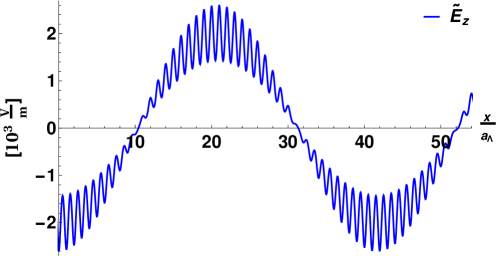
Figure 2: The spatial variation of the microscopic local electric field $\tilde{\mathbf{E}}\left(\mathbf{r},\omega\right)$ representing the solution (74) to the inhomogenous field-integral equations (33) for an external electric field amplitude $\mathbf{\tilde{E}}_{ext}\left(\mathbf{r},\omega_{ext}\right)=\mathbf{e}^{\left(z\right)}\exp\left(i\mathbf{q}\cdot\mathbf{r}\right)\left[\text{$\frac{V}{m}$}\right]$ in the guise of a plane wave, propagating in x - direction and linearly polarized in z - direction. The plot visualizes the rapid spatial variations of the microscopic local electric field traversing a simple cubic crystal along a path $\mathbf{r}\left(x\right)=x\cdot\mathbf{e}^{\left(x\right)}+\frac{a_{\Lambda}}{2}\left(\mathbf{e}^{\left(y\right)}+\mathbf{e}^{\left(z\right)}\right)$ assuming for the external field a vacuum wavelength $\lambda=50\,nm$ in the extreme ultraviolet. A corresponding visualization that applies for visible violet light with vacuum wavelength $\lambda=400\,nm$ is presented in Fig.3.

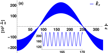
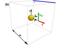
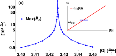
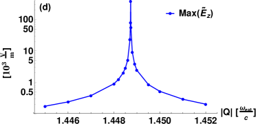
Figure 3: (a) The spatial variation of the microscopic local electric field $\tilde{\mathbf{E}}\left(\mathbf{r},\omega\right)$ representing the solution (74) to the inhomogenous field-integral equations (33) for an external field $\mathbf{\tilde{E}}_{ext}\left(\mathbf{r},\omega_{ext}\right)=\mathbf{e}^{\left(z\right)}\exp\left(i\mathbf{q}\cdot\mathbf{r}\right)\left[\text{$\frac{V}{m}$}\right]$ in the guise of a plane wave, propagating in x - direction and linearly polarized in z - direction. The plot visualizes the rapid spatial variations of the microscopic local electric field traversing a simple cubic crystal along a path $\mathbf{r}\left(x\right)=x\cdot\mathbf{e}^{\left(x\right)}+\frac{a_{\Lambda}}{2}\left(\mathbf{e}^{\left(y\right)}+\mathbf{e}^{\left(z\right)}\right)$ assuming for the external field a vacuum wavelength $\lambda=400\,nm$ corresponding to visible violet light. The applied parameters in (a) are: $a_{\Lambda}=3.5\text{\AA}$, $\frac{\alpha}{4\pi\varepsilon_{0}}=8{\text{\AA}}^{3}$, $\omega_{\text{ext}}=\frac{2\pi c}{\lambda}$ , $n=3.4256$, $\mathbf{q}=\frac{\omega_{\text{ext}}}{c}n\mathbf{e}^{\left(x\right)}$. The inset zooms to a smaller scale so that the spatial variations of the microscopic local electric field are discernible. (b) Schematic illustration of the path along which the spatial variations of the microscopic local electric field are displayed in (a). (c) Depiction of the maximal electric field strenght $\max_{x}\tilde{E}_{z}\left(\mathbf{r}\left(x\right),\omega_{ext}\right)$ along the path $\mathbf{r}\left(x\right)$ as displayed in (b), varying the modulus $Q$ of the wave vector $\mathbf{Q}=Q\,\mathbf{e}^{\left(x\right)}$ of the external field $\mathbf{\tilde{E}}_{ext}\left(\mathbf{r},\omega_{ext}\right)=\mathbf{e}^{\left(z\right)}\exp\left(i\mathbf{Q}\cdot\mathbf{r}\right)\left[\text{$\frac{V}{m}$}\right]$. As is clearly on view, only solutions to the field-integral equations with wave vector $\left|\mathbf{Q}-\mathbf{q}\right|<\delta Q$ meeting the conditions of tolerance set by the solvability condition of the homogeneous field-integral equations, $\omega_{ext}=\omega_{n}\left(\mathbf{Q}\right)$ as shown in the inset of (c), may propagate with sufficient intensity inside the crystal. By increasing the lattice constant to a value of $a_{\Lambda}=5\text{\AA}$, the density of polarizable atoms as well as the witdh $\delta Q$ of the distribution are decreased considerably, see (d).

The result (III) also reveals that the strength of the microscopic local field amplitude inside the crystal strongly depends on the choice of the propagation direction $\mathbf{\hat{q}}=\mathbf{\frac{q}{\left|\mathbf{q}\right|}}$, a feature being directly connected to the photonic band structure implicitely encoded in the eigenvalues of the matrix $\Gamma\left(\mathbf{q},\omega\right)$. The huge size of the induced electric field strength, represented by the difference $\tilde{E}_{a}\left(\mathbf{r},\omega\right)-\tilde{E}_{ext,a}\left(\mathbf{r},\omega\right)$, can indeed be prorated to the predominant longitudinal character of the microscopic local electric field (III) inside a probe volume with a high density of polarizable atoms (ions, molecules). This is intuitively accessible in view of the quasi static electric field inside a material probe at a point $\mathbf{r}\in\Omega_{P}$ originating from nearby positioned induced atomic dipoles.

To elucidate the nature of the microscopic local electric field in (III) and (74) respectively, let us decompose it into longitudinal and transversal parts. With (74) we write now

$$\tilde{E}_{a}^{\left(L,T\right)}\left(\mathbf{r},\omega\right) = \sum_{a^{\prime}}\int d^{3}r^{\prime}\Pi_{a,a^{\prime}}^{\left(L,T\right)}\left(\mathbf{r}^{\prime}\right)\tilde{E}_{a^{\prime}}\left(\mathbf{r}-\mathbf{r}^{\prime},\omega\right)$$

$$= \sum_{a^{\prime}}\bar{\Pi}_{a,a^{\prime}}^{\left(L,T\right)}\left(\mathbf{q}\right)\mathcal{\bar{E}}_{ext,a^{\prime}}\left(\mathbf{q},\omega\right)e^{i\mathbf{q}\cdot\mathbf{r}}$$

$$+\sum_{a^{\prime},a^{\prime\prime},a^{\prime\prime\prime}}\frac{1}{\left|C_{\Lambda}\right|}\sum_{\mathbf{G}\in\Lambda^{-1}}e^{i\left(\mathbf{q}+\mathbf{G}\right)\cdot\mathbf{r}}\bar{\Pi}_{a,a^{\prime}}^{\left(L,T\right)}\left(\mathbf{q}+\mathbf{G}\right)\mathcal{\bar{G}}_{a^{\prime},a^{\prime\prime}}(\mathbf{q}+\mathbf{G},\omega)\left[\bar{K}_{\Lambda}\left(\mathbf{G},\mathbf{q},\omega\right)\right]_{a^{\prime\prime},a^{\prime\prime\prime}}\mathcal{\bar{E}}_{ext,a^{\prime\prime\prime}}\left(\mathbf{q},\omega\right).$$

Taking into account (II) we have

$$\sum_{a^{\prime}}\bar{\Pi}_{a,a^{\prime}}^{\left(L\right)}\left(\mathbf{q}+\mathbf{G}\right)\mathcal{\bar{G}}_{a^{\prime},a^{\prime\prime}}(\mathbf{q}+\mathbf{G},\omega) = -\frac{\left(\mathbf{q}+\mathbf{G}\right)_{a}\left(\mathbf{q}+\mathbf{G}\right)_{a^{\prime\prime}}}{\left|\mathbf{q}+\mathbf{G}\right|^{2}}$$ (77)

$$\sum_{a^{\prime}}\bar{\Pi}_{a,a^{\prime}}^{\left(T\right)}\left(\mathbf{q}+\mathbf{G}\right)\mathcal{\bar{G}}_{a^{\prime},a^{\prime\prime}}(\mathbf{q}+\mathbf{G},\omega) = \frac{\omega^{2}}{c^{2}}\frac{\delta_{a,a^{\prime\prime}}-\frac{\left(\mathbf{q}+\mathbf{G}\right)_{a}\left(\mathbf{q}+\mathbf{G}\right)_{a^{\prime\prime}}}{\left|\mathbf{q}+\mathbf{G}\right|^{2}}}{\left|\mathbf{\mathbf{q}}+\mathbf{G}\right|^{2}-\frac{\omega^{2}}{c^{2}}-i0^{+}}.$$ (78)

The searched-for longitudinal and transversal parts of the microscopic local electric field are thus explicitely determined:

$$\tilde{E}_{a}^{\left(L\right)}\left(\mathbf{r},\omega\right) = \mathcal{\bar{E}}_{ext,a}^{\left(L\right)}\left(\mathbf{q},\omega\right)e^{i\mathbf{q}\cdot\mathbf{r}}$$

$$-\sum_{a^{\prime\prime},a^{\prime\prime\prime}}\frac{1}{\left|C_{\Lambda}\right|}\sum_{\mathbf{G}\in\Lambda^{-1}}e^{i\left(\mathbf{q}+\mathbf{G}\right)\cdot\mathbf{r}}\frac{\left(\mathbf{q}+\mathbf{G}\right)_{a}\left(\mathbf{q}+\mathbf{G}\right)_{a^{\prime\prime}}}{\left|\mathbf{q}+\mathbf{G}\right|^{2}}\left[\bar{K}_{\Lambda}\left(\mathbf{G},\mathbf{q},\omega\right)\right]_{a^{\prime\prime},a^{\prime\prime\prime}}\mathcal{\bar{E}}_{ext,a^{\prime\prime\prime}}\left(\mathbf{q},\omega\right)$$

$$\tilde{E}_{a}^{\left(T\right)}\left(\mathbf{r},\omega\right) = \mathcal{\bar{E}}_{ext,a}^{\left(T\right)}\left(\mathbf{q},\omega\right)e^{i\mathbf{q}\cdot\mathbf{r}}$$

$$+\sum_{a^{\prime\prime},a^{\prime\prime\prime}}\frac{1}{\left|C_{\Lambda}\right|}\sum_{\mathbf{G}\in\Lambda^{-1}}e^{i\left(\mathbf{q}+\mathbf{G}\right)\cdot\mathbf{r}}\frac{\omega^{2}}{c^{2}}\frac{\delta_{a,a^{\prime\prime}}-\frac{\left(\mathbf{q}+\mathbf{G}\right)_{a}\left(\mathbf{q}+\mathbf{G}\right)_{a^{\prime\prime}}}{\left|\mathbf{q}+\mathbf{G}\right|^{2}}}{\left|\mathbf{\mathbf{q}}+\mathbf{G}\right|^{2}-\frac{\omega^{2}}{c^{2}}-i0^{+}}\left[\bar{K}_{\Lambda}\left(\mathbf{G},\mathbf{q},\omega\right)\right]_{a^{\prime\prime},a^{\prime\prime\prime}}\mathcal{\bar{E}}_{ext,a^{\prime\prime\prime}}\left(\mathbf{q},\omega\right)$$

The spatial variations of the transversal amplitude $\tilde{E}_{a}^{\left(T\right)}\left(\mathbf{r},\omega\right)$ and the longitudinal amplitude $\tilde{E}_{a}^{\left(L\right)}\left(\mathbf{r},\omega\right)$ along the same path $\mathbf{r}\left(x\right)$ (and the same parameters as in Fig. 3) is displayed in Fig. 4. It is important to realize that the longitudinal component $\tilde{E}_{a}^{\left(L\right)}\left(\mathbf{r},\omega\right)$ increases rapidly as the density of polarizable atoms (ions, molecules) in the probe volume increases, see Fig.5.

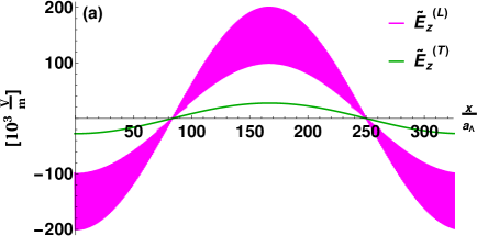
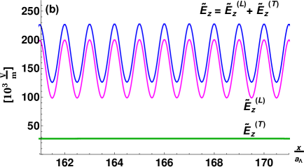
Figure 4: (a) The spatial variation of the z-component $\tilde{E}_{z}^{(L)}\left(\mathbf{r},\omega\right)$ of the longitudinal part of the microscopic local electric field (magenta) and the spatial variation of the z-component $\tilde{E}_{z}^{(T)}\left(\mathbf{r},\omega\right)$ of the transversal part of the microscopic local electric field (green) corresponding to the same parameters as in Fig. 3. The local field $\tilde{E}_{z}\left(\mathbf{r},\omega\right)=\tilde{E}_{z}^{\left(L\right)}\left(\mathbf{r},\omega\right)+\tilde{E}_{z}^{\left(T\right)}\left(\mathbf{r},\omega\right)$ is for a crystal of high particle density (high refractive index), as depicted in (b), dominated by its static longitudinal (dipole) part $\tilde{E}_{z}^{\left(L\right)}\left(\mathbf{r},\omega\right)$, while the tranversal part $\tilde{E}_{z}^{\left(T\right)}\left(\mathbf{r},\omega\right)$ is distinctly smaller.

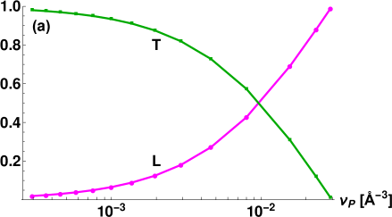
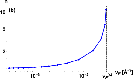
Figure 5: (a) Plot of the ratio of maximum field strengths $\frac{\max_{x}\left|\tilde{E}_{z}^{(L,T)}\left(\mathbf{r}\left(x\right),\omega\right)\right|}{\max_{x}\left|\tilde{E}_{z}\left(\mathbf{r}\left(x\right),\omega\right)\right|}$ vs. particle density $\nu_{P}$ with parameters like in Fig.3. Near to the border of instability at $\nu=\nu_{P}^{\left(c\right)}$ the transversal (radiative) amplitude $\tilde{E}_{z}^{(T)}\left(\mathbf{r},\omega\right)$ is strongly suppressed while the longitudinal amplitude $\tilde{E}_{z}^{\left(L\right)}\left(\mathbf{r},\omega\right)$ becomes large. Conversely, at low particle density $\nu_{P}\rightarrow 0$ the longitudinal amplitude $\tilde{E}_{z}^{\left(L\right)}\left(\mathbf{r},\omega\right)$ vanishes while the transversal amplitude essentially coincides with the field amplitude of the external field. (b) The variation of the index of refraction $n\left(\omega\right)$ vs. the density $\nu_{P}$ of polarizable atoms (ions, molecules) in a dielectric crystal. At the borderline of stability the index of refraction $n\left(\omega\right)$ displays a singularity as $\nu_{P}$ approaches (from below) the critical density $\nu_{P}^{\left(c\right)}$.

Photonic Bandstructure

If no external field was incident, i.e. for $\tilde{\mathfrak{e}}_{ext,a}^{\left(j\right)}\left(\mathbf{q},\omega\right)\equiv 0$, a non trivial field amplitude $\tilde{\mathfrak{e}}_{a}^{\left(j\right)}\left(\mathbf{q},\omega\right)$ solving the homogenous system of equations (63) is obviously identical to an eigenvector $\tilde{\mathfrak{v}}_{a,n}^{\left(j\right)}\left(\mathbf{q},\omega\right)$ associated with the special eigenvalue

$$\gamma_{n}\left(\mathbf{q},\omega\right)=1$$ (81)

of the eigenvalue problem

$$\sum_{j^{\prime}}\sum_{a^{\prime}}\Gamma_{a,a^{\prime}}^{\left(j,j^{\prime}\right)}\left(\mathbf{k},\omega\right)\tilde{\mathfrak{v}}_{a^{\prime},n}^{\left(j^{\prime}\right)}\left(\mathbf{q},\omega\right)=\gamma_{n}\left(\mathbf{q},\omega\right)\tilde{\mathfrak{v}}_{a,n}^{\left(j\right)}\left(\mathbf{q},\omega\right).$$ (82)

The dispersion relation of photons, i.e. the photonic bandstructure $\omega_{n}\left(\mathbf{q}\right)$, can now be readily determined for any number $M$ of basis atoms inside the unit cell $C_{\Lambda}$ by first solving (numerically) the eigenvalue problem (82) for a given wave vector $\mathbf{q}\in C_{\varLambda^{-1}}$ as a function of $\omega$, thus obtaining a family of $3M$ eigenvalue curves $\gamma_{n}\left(\mathbf{q},\omega\right)$ vs. $\omega$, and then solving (numerically) for $n=1,2,3,...3M$ the implicit equations (81) for the unknown $\omega$ so that

$$\left[\gamma_{n}\left(\mathbf{q},\omega\right)-1\right]_{\omega\rightarrow\omega_{n}}=0.$$ (83)

Varying then the wavevector $\mathbf{q}$ along (widely) different symmetry lines inside the Brillouin zone $C_{\Lambda^{-1}}$ various pieces of the photonic bandstructure $\omega_{n}\left(\mathbf{q}\right)$ emerge, as is exemplarily displayed for the diamond lattice ($M=2$) in Fig. 6(a). Like electrons moving in a periodic potential also electromagnetic waves propagating in a crystal are governed by a bandstructure, for example (Leung1990, ; Zhang1990, ; Soezueer1993, ). While the wave function for electrons (discarding spin-orbit forces and Zeeman splitting ) is a scalar, propagating electromagnetic waves are vectorfields. Incident lightsignals composed of frequencies within an omni-directional band gap will be reflected from such a crystal irrespective of the light source being polarized or unpolarized, which is interesting for technical applications, for instance dielectric mirrors, filters or antenna-substrates.

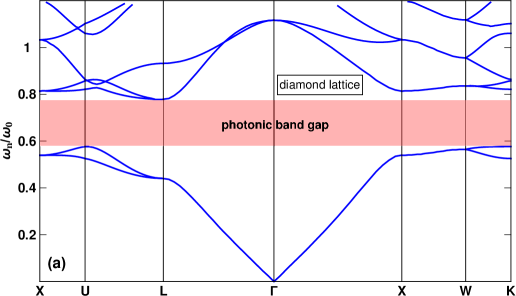
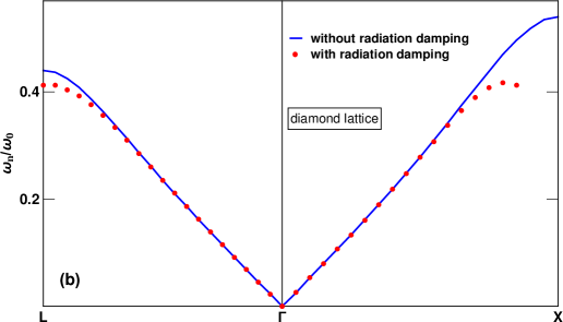
Figure 6: (a) Photonic band structure $\omega_{n}\left(\mathbf{q}\right)$ in units of $\omega_{0}=\frac{2\pi c}{a_{\Lambda}}$ as calculated from (82) for a diamond lattice with wave vector $\mathbf{q}$ orientated along various symmetry lines of the Brillouin zone choosing a lattice constant $a_{\Lambda}=6\text{\AA}$ and assuming a static electronic polarizability $\frac{\alpha_{0}}{4\pi\varepsilon_{0}}=3{\text{\AA}}^{3}$. (b) Taking radiation damping into account, the meaning of the red dots being explained in the supplemental material (Supplementary, ), the photonic band structure $\omega_{n}\left(\mathbf{q}\right)$ of a dielectric crystalline material ceases to make sense approaching the boundary of the Brillouin zone, where $\omega_{n}\left(\mathbf{q}\right)$ enters into the soft x-ray regime.

Further examples of photonic band structures calculated from (82) and (83) with our method, exemplarily for sc-, fcc- and bcc-lattices ($M=1$), are given in supplemental material (Supplementary, ). Our results comply well with calculations carried out within the frame of the Fano-Hopfield model (Klugkist2006, ; Antezza2009, ) in the case of weak coupling of the oscillators. Earlier calculations for super-lattices on the basis of the macroscopic Maxwell equations (Leung1990, ; Zhang1990, ; Soezueer1993, ), carried out in a basis of plane waves $e^{i\left(\mathbf{q}+\mathbf{G}\right)\mathbf{r}}$, require for $\mathbf{q}$ fixed a large number $N$ of reciprocal lattice vectors $\mathbf{G}$ to be taken into account, for accurate computations typically $N\geq 2000$ (Hermann2001, ), thus leading to a huge $3N\times 3N$ matrix eigenvalue problem for the modes and mode freqencies. Unfortunately, these calculations suffer from an inconsistency, as a number $N$ of spurious zero eigenvalue modes needs explicit elimination by an ad hoc transversality constraint. Because in our approach the extension of the scatterers is tiny compared to the lattice constant, our results cease agreement with theirs in certain details of the photonic bandstructure at high photon frequency, while for optical frequencies and below our results are in full agreement with theirs. Regarding the calculational cost of our approach: in the case of sc-, fcc- and bcc-lattices with one atom in the unit cell we solve (for each $\mathbf{q}$-vector) a $3\times 3$ eigenvalue problem, and in the case of diamond with two atoms in the unit cell then a $6\times 6$ eigenvalue problem. Parameters of interest to propagation of light pulses, for instance group velocity and effective photon mass, can be determined conveniently using $k\cdot p$-perturbation theory (Hermann2001, ), a method often employed in solid state electronic band structure theory (Ashcroft1981, ).

Finally, it should be considered that higher bands $n>1$ of the photonic band structure $\omega_{n}\left(\mathbf{q}\right)$ in real crystalline materials are not credibly calculable. While the concept of a photonic band structure exhibiting many band branches $\omega_{n}\left(\mathbf{q}\right)$ certainly applies for (artificial) superlattice structures with large mesoscopic lattice constant $a_{\Lambda}\gg a$, it can be accepted only with reserve for a real dielectric material. This is because for a microscopic lattice constant $a_{\Lambda}\simeq a$ photon frequencies above $\omega\geq\omega_{\Lambda}=c\times\frac{\pi}{a_{\Lambda}}$ are far and beyond the ultra-violet. In this case the effects of radiation damping, as represented by the imaginary part of the lattice sums,

$$\mathtt{Im}\left[\zeta_{\varLambda}^{\left(0\right)}(\mathbf{q},\omega)\right]_{aa^{\prime}}=-\frac{1}{6\pi}\left(\frac{\omega}{c}\right)^{3}\delta_{a,a^{\prime}},$$ (84)

can no longer be neglected. For a derivation of (84) see supplemental material (Supplementary, ). In Fig.6(b) the effect of taking into account radiation damping is exemplarily shown for the diamond lattice ($M=2$). The corresponding plots revealing the influence of radiation damping for the sc-, fcc- and bcc-lattices ($M=1$) we also present in (Supplementary, ). Of course, if the wavelength of the external electromagnetic field is ultra short then the point dipole ansatz (35) for the dielectric susceptibility should be extended to include also magnetic dipoles and electric quadrupoles on equal footing (Raab2005, ).

IV The Dielectric Tensor of Macroscopic Electrodynamics

The macroscopic electric field $\mathcal{\tilde{E}}_{a}\left(\mathbf{r},\omega\right)$ inside the probe we conceive as a low-pass filter applied to the Fourier-transformation $\bar{E}_{a}\left(\mathbf{q},\omega\right)$ of the spatially rapidly varying microscopic local electric field $\tilde{E}_{a}\left(\mathbf{r},\omega\right)$. Introducing a cut-off wavenumber $q_{c}$ so that $q<q_{c}$ implies $\mathbf{q}\in C_{\Lambda^{-1}}$, then

$$\mathcal{\tilde{E}}_{a}\left(\mathbf{r},\omega\right) = \int\frac{d^{3}q}{\left(2\pi\right)^{3}}e^{i\mathbf{q}\cdot\mathbf{r}}\Theta\left(q_{c}-\left|\mathbf{q}\right|\right)\bar{E}_{a}\left(\mathbf{q},\omega\right)$$ (85)

$$\bar{E}_{a}\left(\mathbf{q},\omega\right) = \frac{1}{\left|\Omega_{P}\right|}\int_{\Omega_{P}}d^{3}re^{-i\mathbf{q}\cdot\mathbf{r}}\tilde{E}_{a}\left(\mathbf{r},\omega\right).$$

Likewise, the macroscopic polarization $\mathcal{\tilde{P}}_{a}\left(\mathbf{r},\omega\right)$ inside the probe we conceive as a low-pass filter applied to the Fourier-transformation $\bar{P}_{a}\left(\mathbf{q},\omega\right)$ of the microscopic polarization $\tilde{P}_{a}\left(\mathbf{r},\omega\right)$, as defined in (32):

$$\mathcal{\tilde{P}}_{a}\left(\mathbf{r},\omega\right) = \int\frac{d^{3}q}{\left(2\pi\right)^{3}}e^{i\mathbf{q\cdot}\mathbf{r}}\Theta\left(q_{c}-\left|\mathbf{q}\right|\right)\bar{P}_{a}\left(\mathbf{q},\omega\right)$$ (86)

$$\bar{P}_{a}\left(\mathbf{q},\omega\right) = \frac{1}{\left|\Omega_{P}\right|}\int_{\Omega_{P}}d^{3}re^{-i\mathbf{q}\cdot\mathbf{r}}\tilde{P}_{a}\left(\mathbf{r},\omega\right)$$

Thus in the long wavelength limit the Fourier components $\bar{\mathcal{E}}_{a}\left(\mathbf{q},\omega\right)$ of the macroscopic field $\tilde{\mathcal{E}}_{a}\left(\mathbf{r},\omega\right)$ coincide with those of the microscopic local field, and the Fourier components $\mathcal{\bar{P}}_{a}\left(\mathbf{q},\omega\right)$ of the macroscopic polarization $\mathcal{\tilde{P}}_{a}\left(\mathbf{r},\omega\right)$ coincide with those of the microscopic polarization:

$$\mathcal{\bar{E}}_{a}\left(\mathbf{q},\omega\right) = \Theta\left(q_{c}-\left|\mathbf{q}\right|\right)\bar{E}_{a}\left(\mathbf{q},\omega\right)$$ (87)

$$\mathcal{\bar{P}}_{a}\left(\mathbf{q},\omega\right) = \Theta\left(q_{c}-\left|\mathbf{q}\right|\right)\bar{P}_{a}\left(\mathbf{q},\omega\right)$$ (88)

Restricting to $\left|\mathbf{q}\right|<q_{c}$ we now define the dielectric $3\times 3$ tensor $\left[\varepsilon_{\Lambda}\left(\mathbf{q},\omega\right)\right]_{aa^{\prime}}$ of a crystalline dielectric by requiring the macroscopic polarization being proportional to the macroscopic electric field:

$$\mathcal{\bar{P}}_{a}\left(\mathbf{q},\omega\right)=\varepsilon_{0}\sum_{a^{\prime}\in\left\{x,y,z\right\}}\left[\varepsilon_{\Lambda}\left(\mathbf{q},\omega\right)-I\right]_{aa^{\prime}}\mathcal{\bar{E}}_{a^{\prime}}\left(\mathbf{q},\omega\right)$$ (89)

Insertion of (74) gives an explicit expression determining the Fourier amplitude of the microscopic local electric field:

$$\bar{E}_{a}\left(\mathbf{k},\omega\right) = \frac{1}{\left|\Omega_{P}\right|}\int_{\Omega_{P}}d^{3}re^{-i\mathbf{k}\cdot\mathbf{r}}\tilde{E}_{a}\left(\mathbf{r},\omega\right)$$

$$= \mathcal{\bar{E}}_{ext,a}\left(\mathbf{q},\omega\right)\delta_{\mathbf{k},\mathbf{q}}+\sum_{a^{\prime\prime},a^{\prime\prime\prime}}\frac{1}{\left|C_{\Lambda}\right|}\sum_{\mathbf{G}^{\prime}\in\Lambda^{-1}}\delta_{\mathbf{k},\mathbf{q}+\mathbf{G}^{\prime}}\mathcal{\bar{G}}_{a,a^{\prime\prime}}(\mathbf{q}+\mathbf{G}^{\prime},\omega)\left[\bar{K}_{\Lambda}\left(\mathbf{G}^{\prime},\mathbf{q},\omega\right)\right]_{a^{\prime\prime},a^{\prime\prime\prime}}\mathcal{\bar{E}}_{ext,a^{\prime\prime\prime}}\left(\mathbf{q},\omega\right)$$

Decomposing $\mathbf{k}=\mathbf{k}_{0}+\mathbf{G}$ with $\mathbf{k}_{0}\in C_{\Lambda^{-1}}$ and $\mathbf{G}\in\Lambda^{-1}$ there holds for $\mathbf{q}\in C_{\Lambda^{-1}}$ and $\mathbf{G}^{\prime}\in\Lambda^{-1}$

$$\delta_{\mathbf{k},\mathbf{q}+\mathbf{G}^{\prime}}=\delta_{\mathbf{k}_{0},\mathbf{q}}\delta_{\mathbf{G},\mathbf{G}^{\prime}}.$$ (91)

Therefore

$$\bar{E}_{a}\left(\mathbf{k},\omega\right) = \delta_{\mathbf{k}_{0},\mathbf{q}}\bar{E}_{a}\left(\mathbf{q}+\mathbf{G},\omega\right)$$ (92)

$$\bar{E}_{a}\left(\mathbf{q}+\mathbf{G},\omega\right) = \mathcal{\bar{E}}_{ext,a}\left(\mathbf{q},\omega\right)\delta_{\mathbf{G},\mathbf{0}}+\sum_{a^{\prime\prime},a^{\prime\prime\prime}}\frac{1}{\left|C_{\Lambda}\right|}\mathcal{\bar{G}}_{a,a^{\prime\prime}}(\mathbf{q}+\mathbf{G},\omega)\left[\bar{K}_{\Lambda}\left(\mathbf{G},\mathbf{q},\omega\right)\right]_{a^{\prime\prime},a^{\prime\prime\prime}}\mathcal{\bar{E}}_{ext,a^{\prime\prime\prime}}\left(\mathbf{q},\omega\right)\>.$$ (93)

Let us abbreviate for $\mathbf{G}=\mathbf{0}$:

$$\left[\bar{K}_{\Lambda}(\mathbf{q},\omega)\right]_{a,a^{\prime\prime}}\equiv\left[\bar{K}_{\Lambda}(\mathbf{0},\mathbf{q},\omega)\right]_{a,a^{\prime\prime}}=\sum_{1\leq j,j^{\prime\prime}\leq M}\left(\frac{1}{\varepsilon_{0}}\alpha\left(\mathbf{q},\omega\right)\circ\left[I-\Gamma\left(\mathbf{q},\omega\right)\right]^{-1}\right)_{a,a^{\prime\prime}}^{\left(j,j^{\prime\prime}\right)}$$ (94)

Then for $\mathbf{q}\in C_{\Lambda^{-1}}$:

$$\bar{E}_{a}\left(\mathbf{q},\omega\right) = \sum_{a^{\prime}}\left[I+\frac{1}{\left|C_{\Lambda}\right|}\bar{\mathcal{G}}(\mathbf{q},\omega)\circ\bar{K}_{\Lambda}(\mathbf{q},\omega)\right]_{a,a^{\prime}}\mathcal{\bar{E}}_{ext,a^{\prime}}\left(\mathbf{q},\omega\right)$$ (95)

On the other hand there holds keeping in mind the restriction $\mathbf{q}\in C_{\Lambda^{-1}}$:

$$\bar{P}_{a}\left(\mathbf{q},\omega\right) = \varepsilon_{0}\frac{1}{\left|\Omega_{P}\right|}\int_{\Omega_{P}}d^{3}re^{-i\mathbf{q}\cdot\mathbf{r}}\int_{\Omega_{P}}d^{3}r^{\prime}\sum_{a^{\prime}}\tilde{\chi}_{aa^{\prime}}\left(\mathbf{r},\mathbf{r}^{\prime},\omega\right)\tilde{E}_{a^{\prime}}\left(\mathbf{r}^{\prime},\omega\right)$$

$$= \frac{\varepsilon_{0}}{\left|C_{\Lambda}\right|}\sum_{a^{\prime}}\left[\bar{K}_{\Lambda}(\mathbf{q},\omega)\right]_{a,a^{\prime}}\mathcal{\bar{E}}_{ext,a^{\prime}}\left(\mathbf{q},\omega\right)$$

Restricting to the long wavelength limit $\left|\mathbf{q}\right|<q_{c}$ and thus identifying $\mathcal{\bar{P}}_{a}\left(\mathbf{q},\omega\right)=\bar{P}_{a}\left(\mathbf{q},\omega\right)$ and $\mathcal{\bar{E}}_{a}\left(\mathbf{q},\omega\right)=\bar{E}_{a}\left(\mathbf{q},\omega\right)$, and then combining (95) and (89), a conditional equation determining the macroscopic dielectric tensor $\varepsilon_{\Lambda}\left(\mathbf{q},\omega\right)$ is found

$$\bar{\mathcal{P}}_{a}\left(\mathbf{q},\omega\right) = \varepsilon_{0}\sum_{a^{\prime}}\left[\varepsilon_{\Lambda}\left(\mathbf{q},\omega\right)-I\right]_{aa^{\prime}}\mathcal{\bar{E}}_{a^{\prime}}\left(\mathbf{q},\omega\right)$$

$$= \varepsilon_{0}\sum_{a^{\prime},a^{\prime\prime}}\left[\varepsilon_{\Lambda}\left(\mathbf{q},\omega\right)-I\right]_{aa^{\prime}}\left[I+\frac{1}{\left|C_{\Lambda}\right|}\bar{\mathcal{G}}(\mathbf{q},\omega)\circ\bar{K}_{\Lambda}(\mathbf{q},\omega)\right]_{a^{\prime},a^{\prime\prime}}\mathcal{\bar{E}}_{ext,a^{\prime\prime}}\left(\mathbf{q},\omega\right)$$

$$\stackrel{{\scriptstyle!}}{{=}} \frac{\varepsilon_{0}}{\left|C_{\Lambda}\right|}\sum_{a^{\prime}}\left[\bar{K}_{\Lambda}(\mathbf{q},\omega)\right]_{a,a^{\prime}}\mathcal{\bar{E}}_{ext,a^{\prime}}\left(\mathbf{q},\omega\right).$$

Insisting both lines should be identical for any external field amplitude $\mathcal{\bar{E}}_{ext,a}\left(\mathbf{q},\omega\right)$ immediately leads (with help of elementary matrix algebra) to the identification

$$\varepsilon_{\Lambda}\left(\mathbf{q},\omega\right)-I=\frac{1}{\left|C_{\Lambda}\right|}\bar{K}_{\Lambda}(\mathbf{q},\omega)\circ\left[I+\frac{1}{\left|C_{\Lambda}\right|}\bar{\mathcal{G}}(\mathbf{q},\omega)\circ\bar{K}_{\Lambda}(\mathbf{q},\omega)\right]^{-1}.$$ (97)

This is a central result. The macroscopic dielectric tensor $\left[\varepsilon_{\Lambda}\left(\mathbf{q},\omega\right)\right]_{aa^{\prime}}$ is solely determined by the lattice sums $\tilde{\zeta}_{\varLambda}(\mathbf{s},\mathbf{q},\omega)$ of the Bravais lattice $\Lambda$ under consideration and the individual polarizations $\alpha_{a^{\prime\prime},a^{\prime}}\left(\bm{\eta}^{\left(j^{\prime\prime}\right)},\bm{\eta}^{\left(j^{\prime}\right)},\omega\right)$ of the atoms (ions) inside the unit cell. As a test of the analytic structure of the dielectric function $\varepsilon_{\Lambda}\left(\mathbf{q}=\mathbf{0},\omega\right)$ in the complex frequency domain we checked the Lyddane-Sachs-Teller relation, see Fig. 7. In agreement with general considerations under $\omega\rightarrow-\omega$ the real part of $\varepsilon_{\Lambda}\left(\mathbf{q},\omega\right)$ is an even function of $\omega$ and the imaginary part is an odd one.

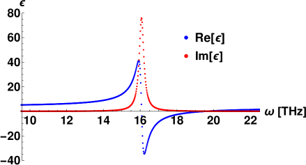
Figure 7: Plot of real and imaginary parts of dielectric function $\varepsilon_{\Lambda}\left(\mathbf{q}=\mathbf{0},\omega\right)\equiv\varepsilon_{\Lambda}\left(\omega\right)$ as calculated from (97) for $CsI$ with microscopic polarizabilities with the parameters from Table 2. The ionic polarizability with frequency dependence given by (38) also includes a small damping parameter $\gamma>0$. The roots of $\text{Re}\left[\varepsilon_{\Lambda}\left(\omega\right)\right]$ are: $\omega_{T}=16.08$THz and $\omega_{L}=19.53$THz, corresponding to frequencies of the transversel and longitudinal optical modes respectively. The zeros of $\text{Re}\left[\varepsilon_{\Lambda}\left(\omega\right)\right]$ obey to the Lyddane-Sachs-Teller relation (Lyddane1941, ), connecting the value of the static dielectric function $\varepsilon_{\Lambda}^{(0)}=4.45$ to its value $\varepsilon_{\Lambda}^{(\infty)}\equiv\varepsilon_{\Lambda}\left(\omega_{T}\cdot 10^{2}\right)=3.05$ above and beyond all optical phonon frequencies: $\frac{\omega_{L}^{2}}{\omega_{T}^{2}}=\frac{\varepsilon_{\Lambda}^{(0)}}{\varepsilon_{\Lambda}^{(\infty)}}$ .

Macroscopic Electric Field

It follows from what has beeen said that the macroscopic electric field amplitude is determined directly from the Fourier series representation (74) discarding all contributions of reciprocal lattice vectors $\mathbf{G}\neq\mathbf{0}$:

$$\mathcal{\tilde{E}}_{a}\left(\mathbf{r},\omega\right) = \sum_{a^{\prime}}\left(\delta_{a,a^{\prime}}+\sum_{a^{\prime\prime}}\frac{1}{\left|C_{\Lambda}\right|}\mathcal{\bar{G}}_{a,a^{\prime\prime}}(\mathbf{q},\omega)\left[\bar{K}_{\Lambda}\left(\mathbf{q},\omega\right)\right]_{a^{\prime\prime},a^{\prime}}\right)\mathcal{\bar{E}}_{ext,a^{\prime}}\left(\mathbf{q},\omega\right)e^{i\mathbf{q}\cdot\mathbf{r}}$$ (98)

In position space then the longitudinal (L) and transversal (T) macroscopic electric field amplitudes read

$$\tilde{\mathcal{E}}_{a}^{\left(L\right)}\left(\mathbf{r},\omega\right) = \mathcal{\bar{E}}_{ext,a}^{\left(L\right)}\left(\mathbf{q},\omega\right)e^{i\mathbf{q}\cdot\mathbf{r}}-\frac{1}{\left|C_{\Lambda}\right|}\sum_{a^{\prime},a^{\prime\prime}}\frac{q_{a}q_{a^{\prime\prime}}}{\left|\mathbf{q}\right|^{2}}\left[\bar{K}_{\Lambda}\left(\mathbf{q},\omega\right)\right]_{a^{\prime\prime},a^{\prime}}\mathcal{\bar{E}}_{ext,a^{\prime}}\left(\mathbf{q},\omega\right)e^{i\mathbf{q}\cdot\mathbf{r}}$$ (99)

$$\tilde{\mathcal{E}}_{a}^{\left(T\right)}\left(\mathbf{r},\omega\right) = \mathcal{\bar{E}}_{ext,a}^{\left(T\right)}\left(\mathbf{q},\omega\right)e^{i\mathbf{q}\cdot\mathbf{r}}+\frac{1}{\left|C_{\Lambda}\right|}\sum_{a^{\prime},a^{\prime\prime}}\frac{\omega^{2}}{c^{2}}\frac{\delta_{a,a^{\prime\prime}}-\frac{q_{a}q_{a^{\prime\prime}}}{\left|\mathbf{q}\right|^{2}}}{\left|\mathbf{\mathbf{q}}\right|^{2}-\frac{\omega^{2}}{c^{2}}-i0^{+}}\left[\bar{K}_{\Lambda}\left(\mathbf{q},\omega\right)\right]_{a^{\prime\prime},a^{\prime}}\mathcal{\bar{E}}_{ext,a^{\prime}}\left(\mathbf{q},\omega\right)e^{i\mathbf{q}\cdot\mathbf{r}}\>.$$ (100)

Comparing now with (III) and (III) we see at once that

$$\tilde{E}_{a}^{\left(L\right)}\left(\mathbf{r},\omega\right) = \tilde{\mathcal{E}}_{a}^{\left(L\right)}\left(\mathbf{r},\omega\right)+\delta\tilde{E}_{a}^{\left(L\right)}\left(\mathbf{r},\omega\right)$$ (101)

$$\delta\tilde{E}_{a}^{\left(L\right)}\left(\mathbf{r},\omega\right) = -\sum_{a^{\prime\prime},a^{\prime\prime\prime}}\frac{1}{\left|C_{\Lambda}\right|}\sum_{\mathbf{G}\neq\mathbf{0}}e^{i\left(\mathbf{q}+\mathbf{G}\right)\cdot\mathbf{r}}\frac{\left(\mathbf{q}+\mathbf{G}\right)_{a}\left(\mathbf{q}+\mathbf{G}\right)_{a^{\prime\prime}}}{\left|\mathbf{q}+\mathbf{G}\right|^{2}}\left[\bar{K}_{\Lambda}\left(\mathbf{G},\mathbf{q},\omega\right)\right]_{a^{\prime\prime},a^{\prime\prime\prime}}\mathcal{\bar{E}}_{ext,a^{\prime\prime\prime}}\left(\mathbf{q},\omega\right)$$

$$\tilde{E}_{a}^{\left(T\right)}\left(\mathbf{r},\omega\right) = \tilde{\mathcal{E}}_{a}^{\left(T\right)}\left(\mathbf{r},\omega\right)+\delta\tilde{E}_{a}^{\left(T\right)}\left(\mathbf{r},\omega\right)$$ (102)

$$\delta\tilde{E}_{a}^{\left(T\right)}\left(\mathbf{r},\omega\right) = \sum_{a^{\prime\prime},a^{\prime\prime\prime}}\frac{1}{\left|C_{\Lambda}\right|}\sum_{\mathbf{G}\neq\mathbf{0}}e^{i\left(\mathbf{q}+\mathbf{G}\right)\cdot\mathbf{r}}\frac{\omega^{2}}{c^{2}}\frac{\delta_{a,a^{\prime\prime}}-\frac{\left(\mathbf{q}+\mathbf{G}\right)_{a}\left(\mathbf{q}+\mathbf{G}\right)_{a^{\prime\prime}}}{\left|\mathbf{q}+\mathbf{G}\right|^{2}}}{\left|\mathbf{\mathbf{q}}+\mathbf{G}\right|^{2}-\frac{\omega^{2}}{c^{2}}-i0^{+}}\left[\bar{K}_{\Lambda}\left(\mathbf{G},\mathbf{q},\omega\right)\right]_{a^{\prime\prime},a^{\prime\prime\prime}}\mathcal{\bar{E}}_{ext,a^{\prime\prime\prime}}\left(\mathbf{q},\omega\right)\>.$$

Accordingly the microscopic local electric field and the macroscopic electric field differ by the contributions of the sums over all reciprocal lattice vectors $\mathbf{G}\neq\mathbf{0}$:

$$\tilde{E}_{a}\left(\mathbf{r},\omega\right) = \tilde{\mathcal{E}}_{a}\left(\mathbf{r},\omega\right)+\delta\tilde{E}_{a}\left(\mathbf{r},\omega\right)$$ (103)

$$\delta\tilde{E}_{a}\left(\mathbf{r},\omega\right) = \sum_{a^{\prime\prime},a^{\prime}}\frac{1}{\left|C_{\Lambda}\right|}\sum_{\mathbf{G}\neq\mathbf{0}}e^{i\left(\mathbf{q}+\mathbf{G}\right)\cdot\mathbf{r}}\mathcal{\bar{G}}_{a,a^{\prime\prime}}(\mathbf{q}+\mathbf{G},\omega)\left[\bar{K}_{\Lambda}\left(\mathbf{G},\mathbf{q},\omega\right)\right]_{a^{\prime\prime},a^{\prime}}\mathcal{\bar{E}}_{ext,a^{\prime}}\left(\mathbf{q},\omega\right)$$

In Fig. 8 we compare the spatial variation of the transversal macroscopic electric field amplitude (100) with the spatial variation of the transversal microscopic local electric field (III) along a path as shown in Fig.3, assuming the external electric field was purely transversal, i.e. $\tilde{\mathcal{E}}_{ext,a}^{\left(L\right)}\left(\mathbf{r},\omega\right)=0$. The residue $\delta\tilde{E}_{z}^{\left(T\right)}\left(\mathbf{r},\omega\right)$ turns out to be smaller by a factor $10^{-5}$ compared to the size of the original amplitudes $\tilde{E}_{z}^{(T)}\left(\mathbf{r},\omega\right)$.

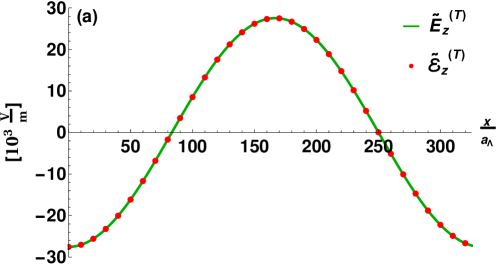
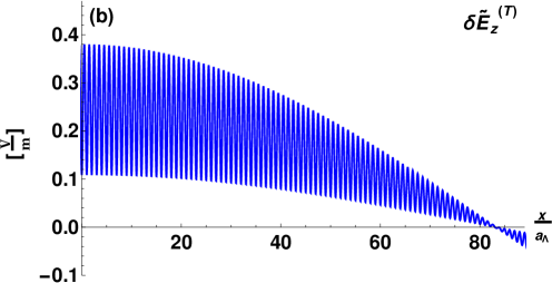
Figure 8: (a) Plot of the transversal part $\tilde{E}_{z}^{(T)}\left(\mathbf{r},\omega\right)$ of the microscopic local electric field (green) and plot of amplitude $\mathcal{\tilde{E}}_{z}^{\left(T\right)}\left(\mathbf{r},\omega\right)$ of the transversal macroscopic field (red dots) along a path $\mathbf{r}\left(x\right)=x\cdot\mathbf{e}^{\left(x\right)}+\frac{a_{\Lambda}}{2}\left(\mathbf{e}^{\left(y\right)}+\mathbf{e}^{\left(z\right)}\right)$ with parameters as in Fig.3, revealing the transversal macroscopic field $\mathcal{\tilde{E}}_{z}^{\left(T\right)}\left(\mathbf{r},\omega\right)$ essentially coincides with the transversal part $E_{z}^{(T)}\left(\mathbf{r},\omega\right)$ of the microscopic local electric field. (b) Plot of the residue $\delta\tilde{E}_{z}^{(T)}\left(\mathbf{r},\omega\right)$ along the same path $\mathbf{r}\left(x\right)$.

Macroscopic Magnetic Induction Field

The amplitude of the microscopic local magnetic induction field $\tilde{\mathbf{B}}\left(\mathbf{r},\omega\right)$ is of course directly connected to the amplitude of the local microscopic electric field $\tilde{\mathbf{E}}\left(\mathbf{r},\omega\right)$ via Faraday’s law:

$$\tilde{\mathbf{B}}\left(\mathbf{r},\omega\right) = \frac{1}{i\omega}\mathbf{\bm{\nabla}}\wedge\tilde{\mathbf{E}}\left(\mathbf{r},\omega\right)$$ (104)

Insertion of the representation (103) for the microscopic local electric field amplitude, $\tilde{E}_{a}\left(\mathbf{r},\omega\right)=\tilde{\mathcal{E}}_{a}\left(\mathbf{r},\omega\right)+\delta\tilde{E}_{a}\left(\mathbf{r},\omega\right)$, leads in this way immediately to

$$\tilde{B}_{c}\left(\mathbf{r},\omega\right) = \sum_{b,a\in\left\{x,y,z\right\}}\frac{1}{i\omega}\epsilon_{cba}\frac{\partial}{\partial r_{b}}\left\{\tilde{\mathcal{E}}_{a}\left(\mathbf{r},\omega\right)+\delta\tilde{E}_{a}\left(\mathbf{r},\omega\right)\right\}\>.$$ (105)

Identifying now the macroscopic magnetic induction field amplitude via

$$\tilde{\mathcal{B}}_{c}\left(\mathbf{r},\omega\right)=\sum_{b,a\in\left\{x,y,z\right\}}\frac{1}{i\omega}\epsilon_{cba}\frac{\partial}{\partial r_{b}}\tilde{\mathcal{E}}_{a}\left(\mathbf{r},\omega\right)$$ (106)

then

$$\tilde{B}_{c}\left(\mathbf{r},\omega\right)=\tilde{\mathcal{B}}_{c}\left(\mathbf{r},\omega\right)+\delta\tilde{B}_{c}\left(\mathbf{r},\omega\right)\>,$$ (107)

where the correction term representing the difference to the microscopic magnetic induction field amplitude is

$$\delta\tilde{B}_{c}\left(\mathbf{r},\omega\right) = \sum_{b,a\in\left\{x,y,z\right\}}\frac{1}{i\omega}\epsilon_{cba}\frac{\partial}{\partial r_{b}}\delta\tilde{E}_{a}\left(\mathbf{r},\omega\right)$$ (108)

$$= \frac{\omega}{c^{2}}\sum_{c^{\prime},c^{\prime\prime},c^{\prime\prime\prime}}\frac{1}{\left|C_{\Lambda}\right|}\sum_{\mathbf{G}\neq\mathbf{0}}e^{i\left(\mathbf{q}+\mathbf{G}\right)\cdot\mathbf{r}}\epsilon_{cc^{\prime}c^{\prime\prime}}\frac{q_{c^{\prime}}+G_{c^{\prime}}}{\left|\mathbf{\mathbf{q}+\mathbf{G}}\right|^{2}-\frac{\omega^{2}}{c^{2}}-i0^{+}}\left[\bar{K}_{\Lambda}\left(\mathbf{G},\mathbf{q},\omega\right)\right]_{c^{\prime\prime},c^{\prime\prime\prime}}\mathcal{\bar{E}}_{ext,c^{\prime\prime\prime}}\left(\mathbf{q},\omega\right)\>.$$

Like in the electric field case, the macroscopic magnetic induction field amplitude $\tilde{\mathcal{B}}_{c}\left(\mathbf{r},\omega\right)$ represents the low pass filtered microscopic local magnetic induction field amplitude $\tilde{B}_{c}\left(\mathbf{r},\omega\right)$. The plot of the residue $\delta\tilde{B}_{y}\left(\mathbf{r},\omega\right)=\tilde{B}_{y}\left(\mathbf{r},\omega\right)-\tilde{\mathcal{B}}_{y}\left(\mathbf{r},\omega\right)$ is displayed in Fig.9. Clearly, $\tilde{B}_{y}\left(\mathbf{r},\omega\right)$ and $\tilde{\mathcal{B}}_{y}\left(\mathbf{r},\omega\right)$ essentially coincide. Note that in the electric field case the relative size of the residue $\delta\tilde{E}_{z}^{\left(T\right)}\left(\mathbf{r},\omega\right)$ along the same path turned out to be even smaller, see Fig.8.

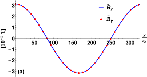
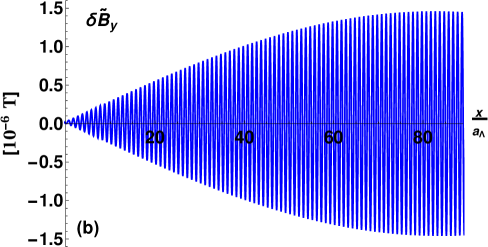
Figure 9: (a) Plot of component $\tilde{B}_{y}\left(\mathbf{r},\omega\right)$ of the microscopic local magnetic induction field amplitude (blue) and plot of component $\mathcal{\tilde{B}}_{y}\left(\mathbf{r},\omega\right)$ of the macroscopic magnetic induction field amplitude (red dots) along a path $\mathbf{r}\left(x\right)=x\cdot\mathbf{e}^{\left(x\right)}+\frac{a_{\Lambda}}{2}\left(\mathbf{e}^{\left(y\right)}+\mathbf{e}^{\left(z\right)}\right)$ with parameters as in Fig.3, revealing that $\mathcal{\tilde{B}}_{y}\left(\mathbf{r},\omega\right)$ essentially coincides with $\tilde{B}_{y}\left(\mathbf{r},\omega\right)$. (b) Plot of the residue $\delta\tilde{B}_{y}\left(\mathbf{r},\omega\right)$ along the same path $\mathbf{r}\left(x\right)$.

Deducing the Differential Equations of Macroscopic Electrodynamics

Restricting to long wavelengths so that $\left|\mathbf{q}\right|<q_{c}$ let us rewrite (95) in the guise

$$\bar{\mathcal{E}}_{a}\left(\mathbf{q},\omega\right)-\mathcal{\bar{E}}_{ext,a}\left(\mathbf{q},\omega\right) = \frac{1}{\left|C_{\Lambda}\right|}\sum_{a^{\prime},a^{\prime\prime}}\bar{\mathcal{G}}_{a,a^{\prime}}(\mathbf{q},\omega)\circ\left[\bar{K}_{\Lambda}(\mathbf{q},\omega)\right]_{a^{\prime},a^{\prime\prime}}\mathcal{\bar{E}}_{ext,a^{\prime\prime}}\left(\mathbf{q},\omega\right)$$

$$= \sum_{a^{\prime},a^{\prime\prime}}\bar{\mathcal{G}}_{a,a^{\prime}}(\mathbf{q},\omega)\circ\left[\varepsilon_{\Lambda}\left(\mathbf{q},\omega\right)-I\right]_{a^{\prime},a^{\prime\prime}}\mathcal{\bar{E}}_{a^{\prime\prime}}\left(\mathbf{q},\omega\right)\>.$$

Multiplication on both sides with the inverse of the kernel (II) gives

$$\sum_{a^{\prime}}\left[\bar{\mathcal{G}}^{-1}(\mathbf{q},\omega)\right]_{a,a^{\prime}}\left[\bar{\mathcal{E}}_{a^{\prime}}\left(\mathbf{q},\omega\right)-\bar{\mathcal{E}}_{ext,a^{\prime}}\left(\mathbf{q},\omega\right)\right]=\sum_{a^{\prime}}\left[\varepsilon_{\Lambda}\left(\mathbf{q},\omega\right)-I\right]_{a,a^{\prime}}\mathcal{\bar{E}}_{a^{\prime}}\left(\mathbf{q},\omega\right)\>.$$ (110)

In terms of the projection operators (8) then

$$\frac{\omega^{2}}{c^{2}}\left[\bar{\mathcal{G}}^{-1}(\mathbf{q},\omega)\right]_{a,a^{\prime}}=\left(\left|\mathbf{q}\right|^{2}-\frac{\omega^{2}}{c^{2}}\right)\bar{\Pi}_{a,a^{\prime}}^{\left(T\right)}\left(\mathbf{q}\right)-\frac{\omega^{2}}{c^{2}}\bar{\Pi}_{a,a^{\prime}}^{\left(L\right)}\left(\mathbf{q}\right)\>,$$ (111)

so that (110) leads to

$$\sum_{a^{\prime}}\left[\left|\mathbf{q}\right|^{2}\bar{\Pi}^{\left(T\right)}\left(\mathbf{q}\right)-\frac{\omega^{2}}{c^{2}}\varepsilon_{\Lambda}\left(\mathbf{q},\omega\right)\right]_{a,a^{\prime}}\bar{\mathcal{E}}_{a^{\prime}}\left(\mathbf{q},\omega\right)=\sum_{a^{\prime}}\left[\left(\left|\mathbf{q}\right|^{2}-\frac{\omega^{2}}{c^{2}}\right)\bar{\Pi}_{a,a^{\prime}}^{\left(T\right)}\left(\mathbf{q}\right)-\frac{\omega^{2}}{c^{2}}\bar{\Pi}_{a,a^{\prime}}^{\left(L\right)}\left(\mathbf{q}\right)\right]\bar{\mathcal{E}}_{ext,a^{\prime}}\left(\mathbf{q},\omega\right)\>.$$ (112)

Identifying transversal and longitudinal components of the Fourier amplitudes of the electric field,

$$\sum_{a^{\prime}}\bar{\Pi}_{a,a^{\prime}}^{\left(L,T\right)}\left(\mathbf{q}\right)\bar{\mathcal{E}}_{ext,a^{\prime}}\left(\mathbf{q},\omega\right) = \bar{\mathcal{E}}_{ext,a}^{\left(L,T\right)}\left(\mathbf{q},\omega\right)$$ (113)

$$\sum_{a^{\prime}}\bar{\Pi}_{a,a^{\prime}}^{\left(L,T\right)}\left(\mathbf{q}\right)\bar{\mathcal{E}}_{a^{\prime}}\left(\mathbf{q},\omega\right) = \bar{\mathcal{E}}_{a}^{\left(L,T\right)}\left(\mathbf{q},\omega\right)$$

let us reexpress the respective Fourier amplitudes of the external electric field in terms of the original sources inside the source domain $\Omega_{S}$, namely the transversal external current distribution $\bar{j}_{ext,a}^{(T)}\left(\mathbf{q},\omega\right)$ and the external charge distribution $\bar{\varrho}_{ext}\left(\mathbf{q},\omega\right)$:

$$\left(\left|\mathbf{q}\right|^{2}-\frac{\omega^{2}}{c^{2}}\right)\bar{\mathcal{E}}_{ext,a}^{\left(T\right)}\left(\mathbf{q},\omega\right) = \mu_{0}i\omega\bar{j}_{ext,a}^{(T)}\left(\mathbf{q},\omega\right)$$ (114)

$$\bar{\mathcal{E}}_{ext,a}^{\left(L\right)}\left(\mathbf{q},\omega\right) = -iq_{a}\bar{\phi}_{ext}\left(\mathbf{q},\omega\right)=-iq_{a}\frac{\bar{\varrho}_{ext}\left(\mathbf{q},\omega\right)}{\varepsilon_{0}\left|\mathbf{q}\right|^{2}}$$ (115)

So the right hand side in (112) reduces together with the Fourier transformed relation (21) to

$$\sum_{a^{\prime}}\left[\left(\left|\mathbf{q}\right|^{2}-\frac{\omega^{2}}{c^{2}}\right)\bar{\Pi}_{a,a^{\prime}}^{\left(T\right)}\left(\mathbf{q}\right)-\frac{\omega^{2}}{c^{2}}\bar{\Pi}_{a,a^{\prime}}^{\left(L\right)}\left(\mathbf{q}\right)\right]\bar{\mathcal{E}}_{ext,a^{\prime}}\left(\mathbf{q},\omega\right) = \left(\left|\mathbf{q}\right|^{2}-\frac{\omega^{2}}{c^{2}}\right)\bar{\mathcal{E}}_{ext,a}^{\left(T\right)}\left(\mathbf{q},\omega\right)-\frac{\omega^{2}}{c^{2}}\bar{\mathcal{E}}_{ext,a}^{\left(L\right)}\left(\mathbf{q},\omega\right)$$ (116)

$$= \mu_{0}i\omega\left[\bar{j}_{ext,a}^{(T)}\left(\mathbf{q},\omega\right)+\bar{j}_{ext,a}^{(L)}\left(\mathbf{q},\omega\right)\right]$$

$$= \mu_{0}i\omega\bar{j}_{ext,a}\left(\mathbf{q},\omega\right)\>.$$ (117)

Consequently (112) assumes the guise

$$\sum_{a^{\prime}}\left[\left|\mathbf{q}\right|^{2}\bar{\Pi}^{\left(T\right)}\left(\mathbf{q}\right)-\frac{\omega^{2}}{c^{2}}\varepsilon_{\Lambda}\left(\mathbf{q},\omega\right)\right]_{a,a^{\prime}}\bar{\mathcal{E}}_{a^{\prime}}\left(\mathbf{q},\omega\right) = \mu_{0}i\omega\bar{j}_{ext,a}\left(\mathbf{q},\omega\right)\>.$$ (118)

If the dependence on wavevector $\mathbf{q}$ of the dielectric tensor in (118) can be ignored, we replace $\varepsilon_{\Lambda}\left(\mathbf{q},\omega\right)\rightarrow\varepsilon_{\Lambda}\left(\omega\right)$ and obtain then in position space the well known (so called) vector wave equation determining the macroscopic electric field:

$$\nabla\wedge\left[\nabla\wedge\tilde{\mathcal{\bm{E}}}\left(\mathbf{r},\omega\right)\right]-\frac{\omega^{2}}{c^{2}}\varepsilon_{\Lambda}\left(\omega\right)\tilde{\mathcal{\bm{E}}}\left(\mathbf{r},\omega\right) = \mu_{0}i\omega\tilde{\mathbf{j}}_{ext}\left(\mathbf{r},\omega\right)$$ (119)

It should be noted, that here $\tilde{\mathcal{\bm{E}}}\left(\mathbf{r},\omega\right)$ still may be decomposed into divergence-free (transversal) and curl-free (longitudinal) parts, $\tilde{\mathcal{\bm{E}}}\left(\mathbf{r},\omega\right)=\tilde{\mathcal{\bm{E}}}^{\left(T\right)}\left(\mathbf{r},\omega\right)+\tilde{\mathcal{\bm{E}}}^{\left(L\right)}\left(\mathbf{r},\omega\right)$. Thus it is deceptive to interpret (119) as a wave equation determining electromagnetic radiation as propagating photons with speed determined by the eigenvalues of the dielectric tensor $\varepsilon_{\Lambda}\left(\omega\right)$, unless $\tilde{\mathcal{\bm{E}}}^{\left(L\right)}\left(\mathbf{r},\omega\right)\equiv\mathbf{0}$.

To find the differential equations for the transversal and longitudinal parts of the macroscopic field amplitude let us first introduce block matrix notation specifying transversal and longitudinal projections of the dielectric tensor:

$$\varepsilon_{a,a^{\prime}}^{\left(A,B\right)}\left(\mathbf{q},\omega\right) = \sum_{b,b^{\prime}}\bar{\Pi}_{a,b}^{\left(A\right)}\left(\mathbf{q}\right)\left[\varepsilon_{\Lambda}\left(\mathbf{q},\omega\right)\right]_{b,b^{\prime}}\bar{\Pi}_{b^{\prime},a^{\prime}}^{\left(B\right)}\left(\mathbf{q}\right)$$ (120)

$$A,B \in \left\{L,T\right\}$$

Then the vector wave equation (118) separates into two coupled equations for the respective transversal and longitudinal Fourier amplitudes of the macroscopic field:

$$\sum_{a^{\prime}}\left(\left|\mathbf{q}\right|^{2}\delta_{a,a^{\prime}}-\frac{\omega^{2}}{c^{2}}\varepsilon_{a,a^{\prime}}^{\left(T,T\right)}\left(\mathbf{q},\omega\right)\right)\bar{\mathcal{E}}_{a^{\prime}}^{\left(T\right)}\left(\mathbf{q},\omega\right)-\frac{\omega^{2}}{c^{2}}\sum_{a^{\prime}}\varepsilon_{a,a^{\prime}}^{\left(T,L\right)}\left(\mathbf{q},\omega\right)\bar{\mathcal{E}}_{a^{\prime}}^{\left(L\right)}\left(\mathbf{q},\omega\right) = \mu_{0}i\omega\bar{j}_{ext,a}^{(T)}\left(\mathbf{q},\omega\right)$$ (121)

$$\sum_{a^{\prime}}\varepsilon_{a,a^{\prime}}^{\left(L,T\right)}\left(\mathbf{q},\omega\right)\bar{\mathcal{E}}_{a^{\prime}}^{\left(T\right)}\left(\mathbf{q},\omega\right)+\sum_{a^{\prime}}\varepsilon_{a,a^{\prime}}^{\left(L,L\right)}\left(\mathbf{q},\omega\right)\bar{\mathcal{E}}_{a^{\prime}}^{\left(L\right)}\left(\mathbf{q},\omega\right) = \bar{\mathcal{E}}_{ext,a}^{\left(L\right)}\left(\mathbf{q},\omega\right)$$

Choosing Eq. (119) as a starting point for the transport theory of radiation (light intensity) inside a (possibly disordered) material appears according to what has been said questionable, as the fluctuation contribution $\tilde{E}_{a}\left(\mathbf{r},\omega\right)-\tilde{\mathcal{E}}_{a}\left(\mathbf{r},\omega\right)\equiv\delta\tilde{E}_{a}\left(\mathbf{r},\omega\right)$, see Eq.(103), is in this case not included, despite the product $\delta\tilde{E}_{a}\left(\mathbf{r},\omega\right)$$\delta\tilde{E}_{b}\left(\mathbf{r}^{\prime},\omega\right)$ apparently comprising a spatially slowly varying interference contribution.

Wave Equation with Renormalized Speed of Light

If the external field was purely transversal, i.e. $\bar{\mathcal{E}}_{ext,a}^{\left(L\right)}\left(\mathbf{q},\omega\right)\equiv 0$, then the longitudinal component of the macroscopic field is readily eliminated in (121), provided the inverse of the longitudinal block $\varepsilon_{\Lambda}^{\left(L,L\right)}\left(\mathbf{q},\omega\right)$ exists:

$$\bar{\mathcal{E}}_{a}^{\left(L\right)}\left(\mathbf{q},\omega\right)=-\sum_{a^{\prime}}\left[\left[\varepsilon^{\left(L,L\right)}\left(\mathbf{q},\omega\right)\right]^{-1}\circ\varepsilon^{\left(L,T\right)}\left(\mathbf{q},\omega\right)\right]_{a,a^{\prime}}\bar{\mathcal{E}}_{a^{\prime}}^{\left(T\right)}\left(\mathbf{q},\omega\right)$$ (122)

Insertion leads to

$$\sum_{a^{\prime}}\left(\left|\mathbf{q}\right|^{2}\delta_{a,a^{\prime}}-\frac{\omega^{2}}{c^{2}}\left[\varepsilon^{\left(T,T\right)}\left(\mathbf{q},\omega\right)-\varepsilon^{\left(T,L\right)}\left(\mathbf{q},\omega\right)\circ\left[\varepsilon^{\left(L,L\right)}\left(\mathbf{q},\omega\right)\right]^{-1}\circ\varepsilon^{\left(L,T\right)}\left(\mathbf{q},\omega\right)\right]_{a,a^{\prime}}\right)\bar{\mathcal{E}}_{a^{\prime}}^{\left(T\right)}\left(\mathbf{q},\omega\right)=\mu_{0}i\omega\bar{j}_{ext,a}^{(T)}\left(\mathbf{q},\omega\right)\>.$$ (123)

Introducing as an effective transversal dielectric tensor

$$\varepsilon^{\left(T\right)}\left(\mathbf{q},\omega\right) = \varepsilon^{\left(T,T\right)}\left(\mathbf{q},\omega\right)-\varepsilon^{\left(T,L\right)}\left(\mathbf{q},\omega\right)\circ\left[\varepsilon^{\left(L,L\right)}\left(\mathbf{q},\omega\right)\right]^{-1}\circ\varepsilon^{\left(L,T\right)}\left(\mathbf{q},\omega\right)\>,$$ (124)

then

$$\sum_{a^{\prime}}\left(\left|\mathbf{q}\right|^{2}\delta_{a,a^{\prime}}-\frac{\omega^{2}}{c^{2}}\varepsilon_{a,a^{\prime}}^{\left(T\right)}\left(\mathbf{q},\omega\right)\right)\bar{\mathcal{E}}_{a^{\prime}}^{\left(T\right)}\left(\mathbf{q},\omega\right)=\mu_{0}i\omega\bar{j}_{ext,a}^{(T)}\left(\mathbf{q},\omega\right)\>.$$ (125)

If the dependence on wavevector $\mathbf{q}$ of the (transversal) dielectric function can be ignored, then $\varepsilon_{ab}^{\left(T\right)}\left(\mathbf{q},\omega\right)\rightarrow\varepsilon_{ab}^{(T)}\left(\omega\right)$, and equation (125) corresponds in position space to a (scalar) wave equation determining the Cartesian components of the transversal macroscopic electric field amplitude $\tilde{\mathcal{\bm{E}}}^{\left(T\right)}\left(\mathbf{r},\omega\right)$ propagating inside a dielectric crystal, in full agreement with the standard theory of the propagation of polarized light in transparent dielectric materials:

$$\sum_{a^{\prime}}\left(-\nabla^{2}\delta_{a,a^{\prime}}-\frac{\omega^{2}}{c^{2}}\varepsilon_{aa^{\prime}}^{(T)}\left(\omega\right)\right)\mathcal{\tilde{E}}_{a^{\prime}}^{\left(T\right)}\left(\mathbf{r},\omega\right)=\mu_{0}i\omega\tilde{j}_{ext,a}^{\left(T\right)}\left(\mathbf{r},\omega\right)$$ (126)

With a choice of a coordinate frame such that the dielectric tensor is diagonal in that frame, $\varepsilon_{aa^{\prime}}^{(T)}\left(\omega\right)=\delta_{aa^{\prime}}n_{a}^{2}\left(\omega\right)$, one finds for light propagating along a high symmetry axis corresponding to an eigenvector of that dielectric tensor the usual reduction of the speed of light, $c\rightarrow c/n_{a}\left(\omega\right)$ characteristic for in general birefringent crystalline dielectrics. Note that because of chromatic dispersion of the index of refraction then those eigenvectors may undergo a corresponding chromatic dispersion of axes as well, yet this effect being observable only for monoclinic and triclinic crystalline symmetry (Born1999, ).

If the dependence on wavevector $\mathbf{q}$ of the (transversal) dielectric function cannot be ignored, the Taylor expansion

$$\varepsilon_{ab}^{\left(T\right)}\left(\mathbf{q},\omega\right)=\varepsilon_{ab}^{\left(T\right)}\left(\omega\right)+i\sum_{c}\gamma_{abc}\left(\omega\right)q_{c}+\sum_{c,d}\alpha_{abcd}\left(\omega\right)q_{c}q_{d}+...$$ (127)

around $\mathbf{q}=\mathbf{0}$ in (125) provides then insight into various optical phenomena connected to retardation and non-locality of the dielectric tensor, in full agreement with the phenomenological reasoning of Agranovich and Ginzburg (Agranovich1984, ): the eigenvalues of the symmetric tensor $\varepsilon_{ab}^{(T)}\left(\omega\right)=\varepsilon_{ba}^{(T)}\left(\omega\right)$ describing chromatic dispersion of the index of refraction and birefringence, the antisymmetric first order term $\gamma_{abc}\left(\omega\right)$ specifying rotary power (natural optical activity), the second order terms $\alpha_{abcd}\left(\omega\right)$ shaping the intrinsic effects of a spatial-dispersion-induced-birefringence. Of course, in a centrosymmetric crystal there exists no natural optical activity: $\gamma_{abc}\left(\omega\right)\equiv 0$. The tensor $\alpha_{abcd}\left(\omega\right)$ originates from the symmetry-breaking evoked by the finite $\mathbf{q}$-vector of the light (Agranovich1984, ), it displays in general $3\times 3\times 3\times 3=81$ components. But for crystals with cubic symmetry the number of independent components of that tensor reduces substantially: for symmetry group $T$ and $T_{h}$ there exist four independent components, for symmetry group $T_{d},$$O_{h}$ and $O$ there exist three independent components and for isotropic systems that number reduces to two (Agranovich1984, ). The (weak) effects of a dispersion-induced-birefringence indeed give as a matter of fact reason for concern regarding the image quality of dielectric lenses made from $CaF_{2}$ and $BaF_{2}$, a topic of prime importance designing modern lithographic optical systems in the ultraviolet (Burnett2002, ; Serebryakov2003, ).

The dielectric tensor $\varepsilon_{\Lambda}\left(\mathbf{q},\omega\right)$ being a functional of the microscopic polarizabilities $\alpha\left(\bm{\eta}^{\left(j\right)},\omega\right)$ of atoms (ions, molecules) located at position $\bm{\eta}^{\left(j\right)}$ in the unit cell $C_{\Lambda}$, for example see (2), undergoes variations in proportion to changes of those atom individual polarizabilities caused by external static fields. For instance, in the presence of a static external magnetic induction field $\mathbf{B}_{0}$, the polarizability of a single atom displays now a magnetic field induced anisotropy (Baranova1979, ), even though the atom-individual polarizability in zero field $\alpha\left(\bm{\eta}^{\left(j\right)},\omega\right)$ was isotropic:

$$\alpha_{aa^{\prime}}\left(\bm{\eta}^{\left(j\right)},\omega;\mathbf{B}_{0}\right) = \left(\left[I+i\frac{\omega}{\left|e\right|}\alpha\left(\bm{\eta}^{\left(j\right)},\omega\right)\circ b\right]^{-1}\circ\alpha\left(\bm{\eta}^{\left(j\right)},\omega\right)\right)_{aa^{\prime}}$$ (128)

$$b_{aa^{\prime}} = \sum_{a^{\prime\prime}}\epsilon_{aa^{\prime}a^{\prime\prime}}B_{a^{\prime\prime}}$$

Such changes then reflect in corresponding changes of the dielectric tensor. As a result the Taylor expansion of the transversal dielectric tensor of the crystal now reads to leading order in the small quantities $\mathbf{q}$ and $\mathbf{B}_{0}$:

$$\varepsilon_{ab}^{\left(T\right)}\left(\mathbf{q},\omega;\mathbf{B}_{0}\right) = \varepsilon_{ab}^{\left(T\right)}\left(\omega\right)+i\sum_{c}\beta_{abc}\left(\omega\right)B_{0,c}+i\sum_{c}\gamma_{abc}\left(\omega\right)q_{c}+...$$ (129)

Note the symmetry

$$\varepsilon_{ab}^{\left(T\right)}\left(-\mathbf{q},\omega;-\mathbf{B}_{0}\right)=\varepsilon_{ba}^{\left(T\right)}\left(\mathbf{q},\omega;\mathbf{B}_{0}\right)\>.$$ (130)

Correspondingly, if the dependence of the transversal dielectric tensor on wavevector $\mathbf{q}$ can be ignored, then light propagation in the presence of a static field $\mathbf{B}_{0}$ inside a dielectric crystal is governed by the wave equation (126), but with a dielectric tensor now dependent on that static magnetic field:

$$\varepsilon_{ab}^{\left(T\right)}\left(\omega;\mathbf{B}_{0}\right)=\varepsilon_{ab}^{\left(T\right)}\left(\omega\right)+i\sum_{c}\beta_{abc}\left(\omega\right)B_{0,c}$$ (131)

The presence of the antisymmetric tensor $\beta_{abc}\left(\omega\right)=\sum_{c^{\prime}}\epsilon_{abc^{\prime}}\lambda_{c^{\prime}c}\left(\omega\right)$ in (131) and with that said in (126), now leads to left and right circularly polarized waves propagating at slightly different speeds, thus giving rise to a magnetic field induced circular birefringence. If $\mathbf{B}_{0}\wedge\mathbf{q}=\mathbf{0}$, i.e. if $\mathbf{B}_{0}$ is orientated parallel or anti-parallel to the direction $\mathbf{\hat{q}}$ of light propagation, this is the well known Faraday rotation effect of a light waves linear polarization in a static magnetic field.

Electric-Field Screening

Conversely, if the external current source was purely longitudinal, i.e. $\bar{j}_{ext,a}^{(T)}\left(\mathbf{q},\omega\right)\equiv 0$, there follows directly from (121) upon elimination of the transversal part $\bar{\mathcal{E}}_{a}^{\left(T\right)}\left(\mathbf{q},\omega\right)$ in favour of the field amplitude $\bar{\mathcal{E}}_{a}^{\left(L\right)}\left(\mathbf{q},\omega\right)$ now the relation

$$\bar{\mathcal{E}}_{a}^{\left(L\right)}\left(\mathbf{q},\omega\right)=\sum_{a^{\prime}}\left(\left[\varepsilon^{\left(L\right)}\left(\mathbf{q},\omega\right)\right]^{-1}\right)_{a,a^{\prime}}\bar{\mathcal{E}}_{ext,a^{\prime}}^{\left(L\right)}\left(\mathbf{q},\omega\right)\>,$$ (132)

with the longitudinal dielectric tensor

$$\varepsilon^{\left(L\right)}\left(\mathbf{q},\omega\right)=\varepsilon^{\left(L,T\right)}\left(\mathbf{q},\omega\right)\circ\frac{\frac{\omega^{2}}{c^{2}}}{\left|\mathbf{q}\right|^{2}I-\frac{\omega^{2}}{c^{2}}\varepsilon^{\left(T,T\right)}\left(\mathbf{q},\omega\right)}\circ\varepsilon^{\left(T,L\right)}\left(\mathbf{q},\omega\right)+\varepsilon^{\left(L,L\right)}\left(\mathbf{q},\omega\right)$$ (133)

describing electric-field screening. From equation (132) we readily infer

$$\sum_{a,a^{\prime}}iq_{a}\varepsilon_{aa^{\prime}}^{\left(L\right)}\left(\mathbf{q},\omega\right)\bar{\mathcal{E}}_{a^{\prime}}^{\left(L\right)}\left(\mathbf{q},\omega\right)=\sum_{a}iq_{a}\bar{\mathcal{E}}_{ext,a}^{\left(L\right)}\left(\mathbf{q},\omega\right)=\frac{\bar{\varrho}_{ext}\left(\mathbf{q},\omega\right)}{\varepsilon_{0}}\>.$$ (134)

For optical frequencies and below it is (obviously) adequate to approximate $\varepsilon^{\left(L\right)}\left(\mathbf{q},\omega\right)\simeq\varepsilon^{\left(L,L\right)}\left(\mathbf{q},\omega\right)$, provided $\det\left[\left|\mathbf{q}\right|^{2}I-\frac{\omega^{2}}{c^{2}}\varepsilon^{\left(T,T\right)}\left(\mathbf{q},\omega\right)\right]\neq 0$. Then

$$\sum_{a,a^{\prime}}iq_{a}\varepsilon_{aa^{\prime}}^{\left(L\right)}\left(\mathbf{q},\omega\right)\bar{\mathcal{E}}_{a^{\prime}}^{\left(L\right)}\left(\mathbf{q},\omega\right) = \sum_{a,a^{\prime}}iq_{a}\varepsilon_{aa^{\prime}}^{\left(L,L\right)}\left(\mathbf{q},\omega\right)\bar{\mathcal{E}}_{a^{\prime}}^{\left(L\right)}\left(\mathbf{q},\omega\right)$$ (135)

$$= \sum_{a,a^{\prime},b,b^{\prime}}iq_{a}\Pi_{ab}^{\left(L\right)}\left(\mathbf{q}\right)\left[\varepsilon_{\Lambda}\left(\mathbf{q},\omega\right)\right]_{bb^{\prime}}\Pi_{b^{\prime}a^{\prime}}^{\left(L\right)}\left(\mathbf{q}\right)\bar{\mathcal{E}}_{a^{\prime}}^{\left(L\right)}\left(\mathbf{q},\omega\right)$$

$$= \sum_{b,b^{\prime}}iq_{b}\left[\varepsilon_{\Lambda}\left(\mathbf{q},\omega\right)\right]_{bb^{\prime}}\bar{\mathcal{E}}_{b^{\prime}}^{\left(L\right)}\left(\mathbf{q},\omega\right)\>.$$

In position space, and representing the longitudinal electric field $\mathcal{\tilde{E}}^{\left(L\right)}\left(\mathbf{r},\omega\right)=-\nabla\tilde{\phi}\left(\mathbf{r},\omega\right)$, this conforms in the long wavelength limit $\mathbf{\left|q\right|}\rightarrow 0$ to the usual Poisson type equation of electrostatics determining the scalar potential $\tilde{\phi}\left(\mathbf{r},\omega\right)$ of a given charge distribution $\tilde{\varrho}_{ext}\left(\mathbf{r},\omega\right)$:

$$\bm{-\nabla}\bm{\mathbf{\cdot}}\left[\varepsilon_{\Lambda}\left(\omega\right)\nabla\tilde{\phi}\left(\mathbf{r},\omega\right)\right]=\frac{\tilde{\varrho}_{ext}\left(\mathbf{r},\omega\right)}{\varepsilon_{0}}$$ (136)

Now it is manifest that it is the dielectric $3\times 3$ tensor

$$\varepsilon_{\Lambda}\left(\omega\right)\equiv\lim_{\left|\mathbf{q}\right|\rightarrow 0}\varepsilon_{\Lambda}\left(\mathbf{q},\omega\right)$$ (137)

that describes electric-field screening, like in electrostatics.

Results of Calculations for the Chromatic Dispersion, Natural Optical Activity and Spatial-Dispersion-Induced Birefringence in Various Dielectric Crystals

Conceiving the polarizability of atoms or ions not as given input from microscopic theory, but as a fit function of the type (36), the diagonal parts depending on two parameters $\omega_{0}^{\left(j\right)}$ and $\alpha_{0}^{\left(j\right)}$ for each atom or ion species $j\in\left\{1,2,...M\right\}$ and also the off diagonal parts depending on two parameters $\omega_{0}^{\left(j,j^{\prime}\right)}$ and $\alpha_{0}^{\left(j,j^{\prime}\right)}$ for each pair $\left(j,j^{\prime}\right)$ of ions $j,j^{\prime}\in\left\{1,2,...M\right\}$ in the unit cell $C_{\Lambda}$, we find the well known Sellmeier fit (Brueckner2011, ) of the frequency dependence of the index of refraction $n\left(\omega\right)$ is nicely reproduced from the eigenvalues of the dielectric tensor $\varepsilon_{ab}^{\left(T\right)}\left(\mathbf{q}=\mathbf{0},\omega\right)$ for a variety of ionic compounds, see exemplarily our results for $CsI$ and $RbCl$ in Fig.10 and $CaF_{2}$ and $BaF_{2}$ in Fig.11. The relative error of our calculations compared to a fit of experimental data for $n\left(\omega\right)$ with the Sellmeier formula for the mentioned crystals is less than 1%.

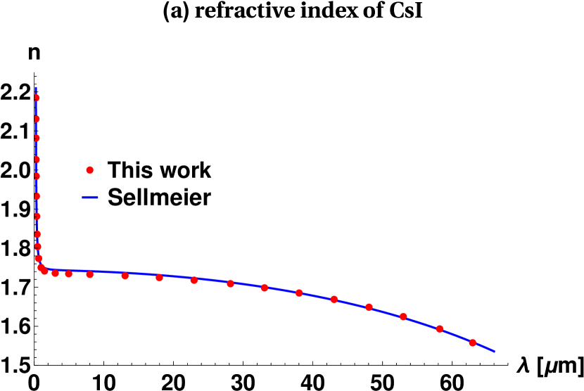
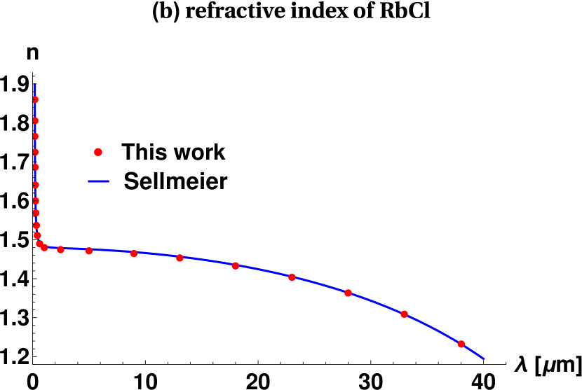
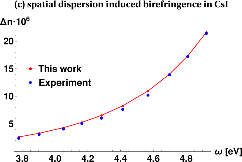
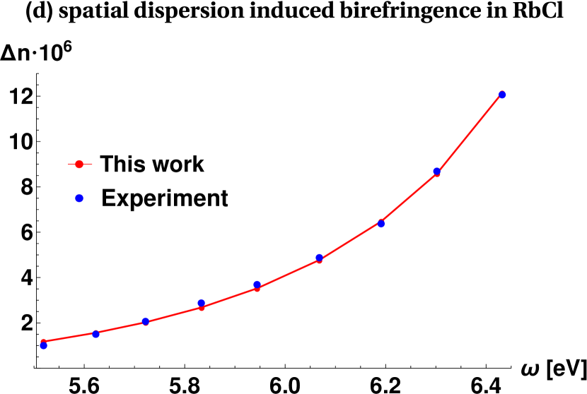
Figure 10: Plot of index of refraction $n\left(\omega\right)$ vs. free space wavelength $\lambda=\frac{2\pi c}{\omega}$ for (a) $CsI$ and (b) $RbCl$. Displayed are values (red dots) calculated from the macroscopic dielectric tensor (97) for $\mathbf{q}=\mathbf{0}$, solely with the lattice symmetry and the microscopic electronic (37) and ionic polarizabilities (38) as input, the respective parameters $\alpha_{0}^{\left(j\right)}$, $\omega_{0}^{\left(j\right)}$,$\alpha_{0}^{\left(j,j^{\prime}\right)}$ and $\omega_{0}^{\left(j,j^{\prime}\right)}$ as listed in Table 2. The relative error compared to a fit of experimental data for $n\left(\omega\right)$ with the multi-parameter Sellmeier formula (Li1976, ) (blue line) is less than 1%. The spatial dispersion induced birefringence $\Delta\text{n}$ as calculated from the $\mathbf{q}$-dependence of the macroscopic dielectric function (97) is displayed (red) in (c) for CsI and (d) for RbCl. To compare with experimental data (Zaldo1986, ) (blue dots) the orientation of the $\mathbf{q}-$vector was chosen along the diagonal of the x-y plane. The estimated error in reading from the plots of the experimental data in (Zaldo1986, ) is about $\pm 0.2\cdot 10^{-6}$.

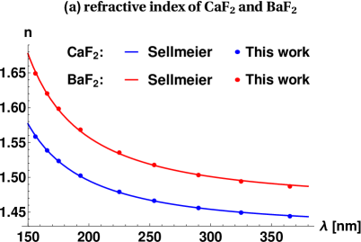
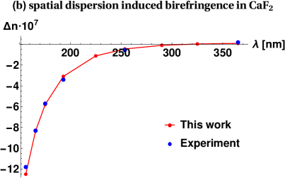
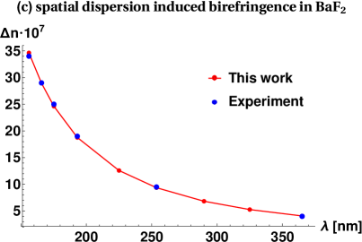
Figure 11: (a) Plot of index of refraction $n\left(\omega\right)$ vs. free space wavelength $\lambda=\frac{2\pi c}{\omega}$ for $CaF_{2}$ and $BaF_{2}$. Displayed are values (dots) calculated from the macroscopic dielectric function (97) for $\mathbf{q}=\mathbf{0}$, solely with the lattice symmetry and the model for electronic polarizabilities (37) as input, the respective values of the parameters $\alpha_{0}^{\left(j\right)}$ and $\omega_{0}^{\left(j\right)}$ as in Table 2. The relative error compared to a fit of experimental data for $n\left(\omega\right)$ with the multi-parameter Sellmeier formula (Li1980, ) (solid lines) is less than 1%. The spatial dispersion induced birefringence $\Delta\text{n}$ as calculated from the $\mathbf{q}$-dependence of the macroscopic dielectric function (97) is displayed (red) in (b) for $CaF_{2}$ and (c) for $BaF_{2}$. To compare with experimental data (Burnett2001, ) (blue dots) the orientation of the $\mathbf{q}-$vector was chosen along the diagonal of the x-y plane.

Let us emphasize our approach warrants notably fewer fit parameters compared to a Sellmeier fit. For example, to reproduce the experimentally observed chromatic dispersion of $CsI$ over a wide frequency intervall, ranging from the ultraviolet to far-infrared, a satisfactory fit to the experimental data within our approach needs only two functions of the type (37) to model the induced electronic polarization of individual ions and a third fit function of the type (38) to model the ionic polarization effect. So our fit relies only on $6$ parameters modelling the microscopic polarizabilities of atoms (ions, molecules, ion pairs) compared, for example, to the $17$ parameters required by the Sellmeier fit (Li1976, ), describing chromatic dispersion of the refractive index of $CsI$.

Furthermore, for (ultraviolet) light propagating along the diagonal of the x-y plane, i.e. $\mathbf{q}=\frac{\left|\mathbf{q}\right|}{\sqrt{2}}\left(\mathbf{e}^{\left(x\right)}+\mathbf{e}^{\left(y\right)}\right)$, the dielectric tensor $\varepsilon_{ab}^{\left(T\right)}\left(\mathbf{q},\omega\right)$ reveals two transversal modes capable to propagate with slightly different speeds inside the crystals mentioned above, thus causing an intrinsic birefringence $\Delta n\left(\omega\right)$ induced by spatial dispersion. Our calculation of $\Delta n\left(\omega\right)$ for the afore mentioned ionic crystals and a comparison with experimental data can be found in Fig.10 and Fig.11. The applied fit parameters entering the calculations of $n\left(\omega\right)$ and $\Delta n\left(\omega\right)$ are listed in Table 2.

Having thus determined the model polarizabilities (37) and (38) for each (different) atom species and each ion pair, the dependence of the dielectric function on wave vector $\mathbf{q}$ is in our approach already fixed by the crystalline structure of the material under consideration, i.e. the rotary power $\gamma_{abc}\left(\omega\right)$ and the dispersion induced anisotropy $\alpha_{abcd}\left(\omega\right)$ are already implicitely encoded in the $\mathbf{q}-$dependence of the transversal dielectric tensor $\varepsilon_{ab}^{\left(T\right)}\left(\mathbf{q},\omega\right)$. To what large extend our calculations agree with published experimental data over a wide range of optical frequencies for a series of quite different crystalline materials we summarize in Table 1, and in particular in Fig. 10 and Fig.11.

While the refractive indices are deduced from the square root of the (real) eigenvalues of the transversal dielectric function for $\mathbf{q}=\mathbf{0}$, the rotary power is determined from the imaginary part of the off-diagonal elements of $\varepsilon_{ab}^{\left(T\right)}\left(\mathbf{q},\omega\right)$ for wave propagation along the crystals’ (optical) z-axis, i.e. $\mathbf{q}=\left|\mathbf{q}\right|\mathbf{e}^{\left(z\right)}$. The examples of crystal structures listed in Table 1 cover the cubic crystal system as well as all uniaxial crystal systems, where the number M of ions comprising the unit cell $C_{\Lambda}$ varies between $M=4$ (for e.g. hexagonal BeO) and $M=66$ (for e.g. cubic $Bi_{12}SiO_{20}$ and $Bi_{12}TiO_{20}$). It should be pointed out, that in contrast to the results shown in Fig.10 and 11, our calculations for the refractive index as well as for the rotary power, both presented in Table 1, solely rest on published data of (anisotropic) electronic polarizabilities being reported in the particular cited references.

As a side remark let us point out, that the described principal effects of non locality, the optical activity $\gamma_{abc}\left(\omega\right)$ and/or the dispersion induced anisotropy $\alpha_{abcd}\left(\omega\right)$, at first sight being small effects compared to $n_{a}^{2}-1$ with $n_{a}^{2}$ representing the eigenvalues of the tensor $\varepsilon_{ab}^{\left(T\right)}\left(\mathbf{q},\omega\right)$ in ordinary crystalline materials, could well be comparable to $n_{a}^{2}-1$ in artificial periodic structures choosing appropriately taylored super lattices, see (Gorlach2016, ).

Table 1: Calculation of the index of refraction $n^{(\text{calc})}$ and rotary power $\rho^{(\text{calc})}$ for wave propagation along the (optical) z-axis for various crystals and comparison with experimental results. The applied data for crystal structures and electronic polarizabilities entering our calculations, as well as the experimental data for the refractive index $n^{(\text{exp})}$ and rotary power $\rho^{(\text{exp})}$ are taken from the publications cited in the column “references”. In case of anisotropic polarizabilities, see e.g. the uniaxial crystals TiO₂ and CaCO₃, $\left[\alpha{}^{\parallel}\right]^{\prime}$ and $\left[\alpha{}^{\perp}\right]^{\prime}$ denote the polarizabilities parallel and perpendicular to the optical z-axis, respectively.

crystal	space group	$\lambda$ (nm)	$\alpha^{\prime}=\frac{\alpha}{4\pi\varepsilon_{0}}$ (Å3)	$n^{(\text{exp})}$	$n^{(\text{calc})}$	$\rho^{(\text{exp})}$ ($\frac{\text{degree}}{\text{mm}}$)	$\rho^{(\text{calc})}$ ($\frac{\text{degree}}{\text{mm}}$)	references
$\alpha$-SiO2	P3121	508	$\alpha^{\prime}_{\text{Si}}=0.207$	$n_{\text{o}}=1.548$	$n_{\text{o}}=1.543$	-29.73	-29.25	(Gualtieri2000, ; Devarajan1986, ; Radhakrishnan1951, ; Lowry, )
			$\alpha^{\prime}_{\text{O}}=1.213$	$n_{\text{e}}=1.558$	$n_{\text{e}}=1.550$
$\beta$-SiO2	P6222	517	$\alpha^{\prime}_{\text{Si}}=0.185$	$n_{\text{o}}=1.536$	$n_{\text{o}}=1.534$	+33.6	+29.84	(Wyckoff, ; Devarajan1986, ; 1962, ; Lowry, )
			$\alpha^{\prime}_{\text{O}}=1.250$	$n_{\text{e}}=1.544$	$n_{\text{e}}=1.539$
TiO2	P42/mnm	589	$\alpha^{\prime}_{\text{Ti}}=0.1862$	$n_{\text{o}}=2.613$	$n_{\text{o}}=2.600$	/	/	(Restori1987, ; Parker1961, ; DeVore1951, )
			$\left[\alpha{}_{O}^{\parallel}\right]^{\prime}=2.6006$	$n_{\text{e}}=2.909$	$n_{\text{e}}=2.921$
			$\left[\alpha{}_{O}^{\perp}\right]^{\prime}=2.2863$
BeO	P63mc	633	$\alpha^{\prime}_{\text{Be}}=0.007$	$n_{\text{o}}=1.717$	$n_{\text{o}}=1.713$	/	/	(Vidal-Valat1987, ; Dimitrov2002, ; Weber, )
			$\alpha^{\prime}_{\text{O}}=1.290$	$n_{\text{e}}=1.732$	$n_{\text{e}}=1.717$
NaClO3	P213	633	$\alpha^{\prime}_{\text{Na}}=0.290$	1.514	1.526	+2.44	+3.76	(Abrahams1977a, ; Devarajan1986, ; Chandrasekhar1967, ; Abrahams1977, )
			$\alpha^{\prime}_{\text{Cl}}=0.010$
			$\alpha^{\prime}_{\text{O}}=1.600$
SrTiO3	Pm$\bar{3}$m	589	$\alpha^{\prime}_{\text{Sr}}=1.0666$	2.410	2.409	/	/	(Abramov1995, ; Chaib2004, ; Weber, )
			$\alpha^{\prime}_{\text{Ti}}=0.1859$
			$\alpha^{\prime}_{\text{O}}=2.3940$
Bi12TiO20	I23	633	$\alpha^{\prime}_{\text{Bi}}=0.0625$	2.562	2.553	-5.9	-6.12	(Swindells1988, ; Weber, ; Feldman1970, )
			$\alpha^{\prime}_{\text{Ti}}=0.272$
			$\alpha^{\prime}_{\text{O}}=3.725$
Bi12SiO20	I23	650	$\alpha^{\prime}_{\text{Bi}}=0.150$	2.52	2.50	-20.5	-19.35	(Abrahams1979a, ; Devarajan1986, ; Weber, ; Abrahams1979, )
			$\alpha^{\prime}_{\text{Si}}=0.001$
			$\alpha^{\prime}_{\text{O}}=3.540$
$\alpha$-AlPO4	P3121	633	$\alpha^{\prime}_{\text{Al}}=0.050$	$n_{\text{o}}=1.524$	$n_{\text{o}}=1.541$	+14.6	+11.23	(Thong1979, ; Devarajan1986, ; Weber, ; Malgrange2014, )
			$\alpha^{\prime}_{\text{P}}=0.050$	$n_{\text{e}}=1.533$	$n_{\text{e}}=1.545$
			$\alpha^{\prime}_{\text{O}}=1.370$
BaTiO3	P4mm	589	$\alpha^{\prime}_{\text{Ba}}=1.9460$	$n_{\text{o}}=2.426$	$n_{\text{o}}=2.400$	/	/	(Xiao2008, ; Chaib2004, ; Wemple1968, )
			$\alpha^{\prime}_{\text{Ti}}=0.1859$	$n_{\text{e}}=2.380$	$n_{\text{e}}=2.380$
			$\alpha^{\prime}_{\text{O}}=2.3940$
CaCO3	R$\bar{3}$cH	589	$\alpha^{\prime}_{\text{Ca}}=0.792$	$n_{\text{o}}=1.658$	$n_{\text{o}}=1.626$	/	/	(Maslen1993, ; Lawless1964, ; Ghosh1999, )
			$\alpha^{\prime}_{\text{C}}=0.000$	$n_{\text{e}}=1.486$	$n_{\text{e}}=1.513$
			$\left[\alpha{}_{\text{O}}^{\left(||\right)}\right]^{\prime}=1.384$
			$\left[\alpha{}_{\text{O}}^{\left(\perp\right)}\right]^{\prime}=1.328$

Table 2: Estimated fit parameters applied to the electronic and ionic Lorentz oscillator models (37) and (38), respectively, regarding our calculations of the refractive index $n\left(\omega\right)$ as well as the spatial-dispersion-induced birefringence $\Delta n\left(\omega\right)$, for ionic crystals $BaF_{2}$, $CaF_{2}$, $CsI$ and $RbCl$.

ion/binding	$\frac{\alpha_{0}}{4\pi\varepsilon_{0}}\;\left[{\text{\AA}}^{3}\right]$	$\omega_{0}\;\left[\text{eV}\right]$
$\text{Ba}^{2+}$	1.577	16.353
$\text{Ca}^{2+}$	0.759	27.484
$\text{Cl}^{-}$	4.500	12.959
$\text{Cs}^{+}$	2.884	33.220
$\text{F}^{-}$ (in $BaF_{2}$)	1.165	15.789
$\text{F}^{-}$ (in $CaF_{2}$)	0.866	15.860
$\text{I}^{-}$	6.241	8.253
$\text{Rb}^{+}$	0.285	7.359
$\text{Cs}^{+}$— $\text{I}^{-}$	1.519	0.012
$\text{Rb}^{+}$— $\text{Cl}^{-}$	2.214	0.019

Static Limit of the Dielectric Function for Monoatomic Bravais Lattices

Assuming for simplicity $M=1$, then there is no loss of generality setting $\bm{\eta}^{\left(1\right)}=\mathbf{0}$. Identifying then, see (57),

$$\alpha_{a^{\prime\prime}a^{\prime}}\left(\omega\right) \equiv \alpha_{a^{\prime\prime},a^{\prime}}^{\left(1,1\right)}\left(\mathbf{k},\omega\right)$$ (138)

$$I_{aa^{\prime}} = \delta_{a,a^{\prime}},$$

one readily infers from (94) the explicit representation

$$\left[\bar{K}_{\Lambda}(\mathbf{q},\omega)\right]_{a^{\prime},a^{\prime\prime}}=\left(\frac{\alpha\left(\omega\right)}{\varepsilon_{0}}\circ\left[I-\zeta_{\varLambda}^{\left(0\right)}(\mathbf{q},\omega)\circ\frac{\alpha\left(\omega\right)}{\varepsilon_{0}}\right]^{-1}\right)_{a^{\prime},a^{\prime\prime}}.$$ (139)

Elementary matrix algebra leads then to the result

$$\varepsilon_{\Lambda}\left(\mathbf{q},\omega\right)-I$$ (140)

$$= \frac{1}{\left|C_{\Lambda}\right|}\frac{\alpha\left(\omega\right)}{\varepsilon_{0}}\circ\left[I-\zeta_{\varLambda}^{\left(0\right)}(\mathbf{q},\omega)\circ\frac{\alpha\left(\omega\right)}{\varepsilon_{0}}\right]^{-1}\circ\left[I+\frac{1}{\left|C_{\Lambda}\right|}\bar{\mathcal{G}}(\mathbf{q},\omega)\circ\frac{\alpha\left(\omega\right)}{\varepsilon_{0}}\circ\left[I-\zeta_{\varLambda}^{\left(0\right)}(\mathbf{q},\omega)\circ\frac{\alpha\left(\omega\right)}{\varepsilon_{0}}\right]^{-1}\right]^{-1}$$

$$= \frac{1}{\left|C_{\Lambda}\right|}\frac{\alpha\left(\omega\right)}{\varepsilon_{0}}\circ\left[I-\left(\zeta_{\varLambda}^{\left(0\right)}(\mathbf{q},\omega)-\frac{1}{\left|C_{\Lambda}\right|}\bar{\mathcal{G}}(\mathbf{q},\omega)\right)\circ\frac{\alpha\left(\omega\right)}{\varepsilon_{0}}\right]^{-1}.$$

In the supplemental material (Supplementary, ) it is shown that

$$\left(\zeta_{\varLambda}^{\left(0\right)}(\mathbf{q},\omega)-\frac{1}{\left|C_{\Lambda}\right|}\bar{\mathcal{G}}(\mathbf{q},\omega)\right)_{a,a^{\prime}}$$

$$= \lim_{\left|\mathbf{s}\right|\rightarrow 0^{+}}\left(\frac{1}{\left|C_{\Lambda}\right|}\sum_{\mathbf{G}\in\Lambda^{-1}\setminus\left\{\mathbf{0}\right\}}e^{i\mathbf{\mathbf{G}}\cdot\mathbf{s}}\frac{\frac{\omega^{2}}{c^{2}}\delta_{a,a^{\prime}}-\left(\mathbf{G}+\mathbf{q}\right)_{a}\left(\mathbf{G}+\mathbf{q}\right)_{a^{\prime}}}{\left|\mathbf{\mathbf{\mathbf{G}+\mathbf{q}}}\right|^{2}-\frac{\omega^{2}}{c^{2}}-i0^{+}}-\int\frac{d^{3}k}{\left(2\pi\right)^{3}}e^{i\mathbf{k}\cdot\mathbf{s}}\frac{\frac{\omega^{2}}{c^{2}}\delta_{a,a^{\prime}}-k_{a}k_{a^{\prime}}}{\left|\mathbf{k}\right|^{2}-\frac{\omega^{2}}{c^{2}}-i0^{+}}\right).$$

The lattice sum (IV) is conveniently evaluated along the lines indicated by Ewald (Ewald1916, ; Ewald1938, ), splitting the sum into two absolutely converging sums, one converging rapidly in the Fourier domain and the other converging rapidly in the spatial domain. For details and a discussion of our (modified) splitting method, see supplemental material (Supplementary, ). For simple cubic lattices the expression (IV) can also be evaluated employing Jacobi theta functions (Draine1993, ; Borwein2013, ).

In the static limit, first $\left|\mathbf{q}\right|\rightarrow 0$ and then $\omega\rightarrow 0$, we write

$$\lim_{\omega\rightarrow 0}\lim_{\left|\mathbf{q}\right|\rightarrow 0}\left[\varepsilon_{\Lambda}\left(\mathbf{q},\omega\right)-I\right]_{a,a^{\prime}}=\left[\varepsilon_{\Lambda}-I\right]_{a,a^{\prime}}.$$ (142)

A comprehensive analysis of the general properties of electromagnetic response functions, quite apart from a particular model description of a material and only based on general principles such as causality and thermodynamic stability, has been given by Kirzhnitz (Kirzhnitz2012, ), who derived for the isotropic case $\left[\varepsilon_{\Lambda}\right]_{a,a^{\prime}}=\varepsilon I_{a,a^{\prime}}$ as a lower bound of allowed static values of the dielectric function:

$$\varepsilon \geq 1$$ (143)

Introducing the (dimensionless) Lorentz factors

$$\mathcal{L}_{a,a^{\prime}}=\left|C_{\Lambda}\right|\lim_{\omega\rightarrow 0}\lim_{\left|\mathbf{q}\right|\rightarrow 0}\left[\zeta_{\varLambda}^{\left(0\right)}(\mathbf{q},\omega)-\frac{1}{\left|C_{\Lambda}\right|}\bar{\mathcal{G}}(\mathbf{q},\omega)\right]_{a,a^{\prime}},$$ (144)

solely dependent on the lattice geometry, and identifying $\frac{1}{\left|C_{\Lambda}\right|}=\frac{\left|\Lambda_{P}\right|}{\left|\Omega_{P}\right|}=\nu_{P}$ with the density of polarizable atoms in the probe volume, there follows from (140) for mono-atomic Bravais lattices $(M=1)$ the following exact formula for the static dielectric tensor:

$$\left[\varepsilon_{\Lambda}\right]_{a,a^{\prime}}=\left[\frac{I+(I-\mathcal{L})\frac{\alpha}{\varepsilon_{0}}\nu_{P}}{I-\mathcal{L}\frac{\alpha}{\varepsilon_{0}}\nu_{P}}\right]_{a,a^{\prime}}$$ (145)

While the polarizability $\alpha$ refers to individual atomic (ionic, molecular) properties, the dielectric tensor $\varepsilon_{\Lambda}$ also depends via the $3\times 3$ matrix of Lorentz factors $\mathcal{L}$ on how the atoms are assembled to build the crystal $\Lambda$. Note that the particle density $\nu_{P}$ of a dielectric crystalline probe volume is bounded from above by the a critical value $\nu_{P}^{\left(c\right)}$,

$$\nu_{P} < \nu_{P}^{\left(c\right)}\equiv\frac{1}{\mathcal{L}_{max}}\frac{\varepsilon_{0}}{\alpha}\;,$$ (146)

with $\mathcal{L}_{max}$ denoting the largest positive eigenvalue of the matrix $\mathcal{L}$. This condition indeed implies the matrix $\varepsilon_{\Lambda}-I$ being positive definit, thus generalizing the stability criterion (143) to the anisotropic case.

It should be noted that the trace of the matrix $\mathcal{L}$ as defined in (144) is normalized to unity:

$$\textrm{tr}\left(\mathcal{L}\right)=1$$ (147)

For a proof see supplemental material (Supplementary, ). Numerical values for the Lorentz factors are readily calculated for all $14$ monoatomic Bravais lattices $\Lambda$ along the lines indicated in the supplemental material (Supplementary, ).

In the special case of a lattice with tetragonal or hexagonal symmetry the matrix $\mathcal{L}$ becomes diagonal, $\mathcal{L}_{a,a^{\prime}}=\delta_{a,a^{\prime}}\mathcal{L}_{a}$. In this case the trace identity (147) leads to $\mathcal{L}_{x}=\mathcal{L}_{y}=\frac{1}{2}\left(1-\mathcal{L}_{z}\right)$, with $\mathcal{L}_{z}$ being a universal function, solely dependent on the ratio $\frac{a_{z}}{a_{x}}$ of the lattice constants, $a_{z}$ parallel and $a_{x}$ perpendicular to the crystalline $z-$axis. In Fig. 12 that function $\mathcal{L}_{z}$ is plotted vs. the ratio of lattice constants $\frac{a_{z}}{a_{x}}$ for simple tetragonal (st), body-centered tetragonal (bct) and also hexagonal (hex) lattice symmetry. Our results for the Lorentz-factors obtained with Eq. (144) coincide with previous works, for example (Colpa1971a, ; Colpa1971, ; Vanzo2014, ).

Figure 12: Plot of Lorentz factor $\mathcal{L}_{z}$ for simple tetragonal (blue), body-centered tetragonal (red) and hexagonal (green) lattice symmetries vs. the ratio $\frac{a_{z}}{a_{x}}$ of lattice constants. The inset shows a zoom into the region where $\mathcal{L}_{z}$ assumes a value around $\frac{1}{3}$, characteristic for isotropic systems.

Clausius-Mossotti Relation

For cubic symmetry there holds $\mathcal{L}_{a,a^{\prime}}=\frac{1}{3}\delta_{a,a^{\prime}}$ and the static dielectric tensor (145) reduces to the well known Clausius-Mossotti relation for isotropic systems, see supplemental material (Supplementary, ):

$$\left[\varepsilon_{\Lambda}\right]_{a,a^{\prime}} = \delta_{a,a^{\prime}}\frac{1+\frac{2}{3}\frac{\alpha}{\varepsilon_{0}}\nu_{P}}{1-\frac{1}{3}\frac{\alpha}{\varepsilon_{0}}\nu_{P}}$$ (148)

Incidentally, the relation (148) applies for a wide class of (isotropic, non polar) materials, including dielectric liquids and gases. On a final note: our derivation of (148) completely avoids the usual trick of introducing the Lorentz sphere, where the medium outside of this sphere is considered as a continuum. For an in-depth explanation of that trick see for example (Ashcroft1981, ).

V Conclusions

The field-integral equation approach presented in this article differs from traditional presentations of crystal optics, for example (Authier2012, ; Born1999, ; Fluegge2013, ). Based on the Helmholtz-Hodge theorem the source term in the microscopic Maxwell equations representing the current density has been decomposed into longitudinal and transversal parts, thus establishing the formulation of equivalent (inhomogenous) field-integral equations with a kernel modelling the induced microscopic polarization $\mathbf{\tilde{P}}\left(\mathbf{r},\omega\right)$ inside a dielectric crystal as a convolution integral of the dielectric susceptibility $\chi_{aa^{\prime}}\left(\mathbf{r},\mathbf{r}^{\prime},\omega\right)$ (35) and the Fourier amplitude $\mathbf{\tilde{E}}\left(\mathbf{r},\omega\right)$ of the microscopic local electric field, see (32). Exploiting the lattice periodicity of the dielectric susceptibility tensor $\chi_{aa^{\prime}}\left(\mathbf{r}+\mathbf{R},\mathbf{r}^{\prime}+\mathbf{R},\omega\right)=\chi_{aa^{\prime}}\left(\mathbf{r},\mathbf{r}^{\prime},\omega\right)$ it is then natural to expand the field amplitude $\mathbf{\tilde{E}}\left(\mathbf{r},\omega\right)$ into a complete and orthonormal basis of eigenfunctions of the operator $T_{\mathbf{R}}$ generating translations by a lattice vector $\mathbf{R}\in\Lambda$, see (41). But instead of expanding the solution to the field-integral equations in the well known basis of plane waves $e^{i\left(\mathbf{q}+\mathbf{G}\right)\mathbf{r}}$, constructed from eigenfunctions of the momentum operator, thus requiring to handle for each wave vector $\mathbf{q}$ in the Brillouin zone $C_{\Lambda^{-1}}$ of the lattice $\Lambda$ then (infinite dimensional) matrices labelled by reciprocal lattice vectors $\mathbf{G},\mathbf{G}^{\prime}\in\Lambda^{-1}$, we use non-standard Bloch functions representing a complete and orthonormal system of eigenfunctions of the translation operator $T_{\mathbf{R}}$ constructed from eigenfunctions of the position operator, see (50). Our choice of basis functions indeed enables to sidesteps the inversion (and truncation) of large matrices with regard to the reciprocal lattice vectors $\mathbf{G},\mathbf{G}^{\prime}\in\Lambda^{-1}$, thus easing significantly the numerical effort.

Considering the homogenous field-integral equations the electromagnetic modes and the photonic band structure $\omega_{n}\left(\mathbf{q}\right)$ of a dielectric crystal have been identified solving a small sized $3M\times 3M$ matrix eigenvalue problem, with $M$ denoting the number of polarizable atoms (ions, molecules) in the elementary cell $C_{\Lambda}$ of the lattice. A radiation damping term $\propto\omega^{3}$, that originates not from the damping terms in the atom-individual polarizabilities (2), but from the retarded Helmholtz propagator evaluating the lattice sum without the self field term, see (84), has been taken into account in all our calculations. Exemplarily we then presented the photonic band structure of diamond ($M=2$). An overview of our results for the photonic bandstructure of (primitive) sc-, fcc- and bcc lattices we present in the supplemental material (Supplementary, ). In all cases we find quantitative agreement with previously published work on photonic band structures calculated with other methods.

Considering the inhomogenous field-integral equations, choosing a (circular) frequency $\omega$ and a wavevector $\mathbf{q}$ obeying to $\omega=\omega_{n}\left(\bm{q}\right)$, the microscopic local electric field amplitude $\mathbf{\tilde{E}}\left(\mathbf{r},\omega\right)$ in the presence of a slowly varying time harmonic external field with amplitude $\mathbf{\tilde{E}}_{ext}\left(\mathbf{r},\omega\right)$ is found to display in general a radiative transversal part (T) and also a longitudinal part (L), the size of the longitudinal amplitude $\mathbf{\tilde{E}}^{\left(L\right)}\left(\mathbf{r},\omega\right)$, see (III), compared to the size of the transversal amplitude $\mathbf{\tilde{E}}^{\left(T\right)}\left(\mathbf{r},\omega\right)$, see (III), being strongly depend on the density of polarizable atoms (ions, molecules) in the crystal, see Fig.5. In a sufficiently dense packed dielectric crystal we find the longitudinal amplitude $\mathbf{\tilde{E}}^{\left(L\right)}\left(\mathbf{r},\omega\right)$ being substantially larger compared to the transversal amplitude $\mathbf{\tilde{E}}^{\left(T\right)}\left(\mathbf{r},\omega\right)$, but in a dilute (artificial) superlattice with polarizable subunits positioned at the lattice sites the longitudinal field amplitude becomes small compared to the transversal one, see Fig.5. While the microscopic local electric field amplitude $\mathbf{\tilde{E}}\left(\mathbf{r},\omega\right)$ displays inside a densely packed lattice rapid spatial variations with large amplitude traversing a distance set by the microscopic inter-particle distance $a$, it turns out that the transversal (radiative) part $\mathbf{\tilde{E}}^{\left(T\right)}\left(\mathbf{r},\omega\right)$ essentially coincides with the slowly varying macroscopic electric field amplitude $\mathcal{\bm{\tilde{E}}}\left(\mathbf{r},\omega\right)$, that field $\mathbf{\tilde{\mathcal{\bm{E}}}}\left(\mathbf{r},\omega\right)$ being conceived as the low pass filtered microscopic local field amplitude, see (85). If the external field $\mathbf{\tilde{E}}_{ext}\left(\mathbf{r},\omega\right)$ was purely transversal and slowly varying, then the amplitude of the residue $\delta\mathbf{\tilde{E}}^{\left(T\right)}\left(\mathbf{r},\omega\right)=\mathbf{\tilde{E}}^{\left(T\right)}\left(\mathbf{r},\omega\right)-\mathbf{\tilde{\mathcal{\bm{E}}}}^{\left(T\right)}\left(\mathbf{r},\omega\right)$ is tiny, see Fig.8.

Conceiving correspondingly the macroscopic Polarization $\tilde{\mathcal{\bm{P}}}\left(\mathbf{r},\omega\right)$ as the low pass filtered microscopic polarization $\mathbf{\tilde{P}}\left(\mathbf{r},\omega\right)$, see (86), then the dielectric $3\times 3$ tensor $\varepsilon_{\Lambda}\left(\mathbf{q},\omega\right)$ of macroscopic electrodynamics emerges from the requirement $\bar{\mathcal{\bm{P}}}\left(\mathbf{q},\omega\right)=\varepsilon_{0}\left[\varepsilon_{\Lambda}\left(\mathbf{q},\omega\right)-I\right]\mathcal{\bar{E}}\left(\mathbf{q},\omega\right)$, with $\bar{\mathcal{\bm{P}}}\left(\mathbf{q},\omega\right)$ and $\mathcal{\bar{E}}\left(\mathbf{q},\omega\right)$ denoting the spatial Fourier transformation of those amplitudes. The derived exact formula for the dielectric tensor $\varepsilon_{\Lambda}\left(\mathbf{q},\omega\right)$, see (97), then solely depends on the microscopic polarizabilities $\alpha_{aa^{\prime}}\left(\bm{\eta}^{\left(j\right)},\bm{\eta}^{\left(j^{\prime}\right)},\omega\right)$ of atoms (molecules, ions) together with the crystalline symmetry $\Lambda$ as input into the theory.

Regarding the propagation of light signals inside a dielectric crystal then the question was clarified, which parts of the dielectric tensor $\varepsilon_{\Lambda}\left(\mathbf{q},\omega\right)$ describe the renormalization of the speed of light and possibly birefringence, chromatic dispersion, rotary power and spatial-dispersion induced birefringence, and which parts govern electric-field screening. Accordingly we derived directly from the field-integral equations, see (IV), a set of (coupled) differential equations for the longitudinal and transversal components determining the macroscopic electric field $\mathcal{\bm{\tilde{E}}}\left(\mathbf{r},\omega\right)$ directly, without any prior knowledge of the microscopic local electric field $\mathbf{\tilde{E}}\left(\mathbf{r},\omega\right)$. If the external field was purely transversal then an effective wave equation for the transversal (radiative) macroscopic field emerged, thus identifying the pieces of $\varepsilon_{\Lambda}\left(\mathbf{q},\omega\right)$ comprising the transversal dielectric tensor $\varepsilon_{aa^{\prime}}^{\left(T\right)}\left(\mathbf{q},\omega\right)$ , see (124). Conversely, if the external field was purely longitudinal, then an effective Poisson type equation for a scalar potential $\tilde{\phi}\left(\mathbf{r},\omega\right)$ turned up, so that the longitudinal macroscopic field is represented by $\mathbf{\tilde{\mathcal{\bm{E}}}}^{\left(L\right)}\left(\mathbf{r},\omega\right)=-\bm{\nabla}\tilde{\phi}\left(\mathbf{r},\omega\right)$, thus identifying the pieces of the dielectric tensor comprising the longitudinal dielectric tensor $\varepsilon_{aa^{\prime}}^{\left(L\right)}\left(\mathbf{q},\omega\right)$ being liable for electric-field screening (like in electrostatics), see (133). In the static limit, $\mathbf{q}\rightarrow\mathbf{0}$ and $\omega\rightarrow 0$, an exact expression for the dielectric tensor $\varepsilon_{\Lambda}$ is derived that applies for all $14$ mono-atomic Bravais lattices, see (145). Our result for $\varepsilon_{\Lambda}$ in particular conforms with general (thermodynamic) stability criteria (Kirzhnitz2012, ), and for cubic symmetry the well known Clausius-Mossotti relation is recovered.

The Taylor expansion of the transversal dielectric tensor, $\varepsilon_{ab}^{\left(T\right)}\left(\mathbf{q},\omega\right)=\varepsilon_{ab}^{\left(T\right)}\left(\omega\right)+i\sum_{c}\gamma_{abc}\left(\omega\right)q_{c}+\sum_{c,d}\alpha_{abcd}\left(\omega\right)q_{c}q_{d}+..$ around $\mathbf{q}=\mathbf{0}$, provides then insight into various optical phenomena connected to retardation and non locality of the dielectric response, in full agreement with the phenomenological reasoning of Agranovich and Ginzburg (Agranovich1984, ): the eigenvalues of the tensor $\varepsilon_{ab}^{\left(T\right)}\left(\omega\right)$ describing chromatic dispersion of the index of refraction and birefringence, the first order term $\gamma_{abc}\left(\omega\right)$ specifying rotary power (natural optical activity) in crystals lacking inversion symmetry, the second order term $\alpha_{abcd}\left(\omega\right)$ shaping the (weak) effects of a spatial-dispersion induced birefringence, nowadays a critical parameter for the design of lenses made from $CaF_{2}$ and $BaF_{2}$ for optical lithograpy systems in the ultraviolet.

Considering various dielectric crystalline materials comprising atoms (molecules, ions) with known polarizabilities from the literature, in all cases the calculated indices of refractions, the rotary power and the dispersion induced birefringence have been shown to coincide well with the experimental data displayed in table 1, thus illustrating the utility of the theory. For ionic crystals, exemplarily for $CsI$ and $RbCl$, a satisfactory agreement between theory and the measured chromatic dispersion of the index of refraction is manifest over a wide frequency interval, ranging from ultraviolet to far infra-red, accomplishing this with an appreciably smaller number of adjustable parameters directly linked to microscopic atomindividual polarizabilities compared to the well known Sellmeier fit. Further we computed for the cubic fluorites $CaF_{2}$ and $BaF_{2}$ the frequency dependence of the intrinsic birefingence, as represented by three independent components of the tensor $\alpha_{abcd}\left(\omega\right)$, and found good agreement with published data (Burnett2001, ; Burnett2002, ).

Even though all our calculations are based on a phenomenological model of microscopic polarizabilities, see (37) and (38), due to the conformity with the fundamental frequency dependence of atom-individual polarizabilities as predicted by quantum mechanics, see (2), our results for the dielectric tensor $\varepsilon_{\Lambda}\left(\mathbf{q},\omega\right)$ may well claim general validity in the range of optical frequencies and below. While the frequency dependence of $\varepsilon_{\Lambda}\left(\mathbf{q},\omega\right)$ is deeply anchored in the retarded response of polarizable atoms (ions, molecules) comprising a dielectric crystal, the dependence of $\varepsilon_{\Lambda}\left(\mathbf{q},\omega\right)$ on the wave vector $\mathbf{q}$ of the propagating light describes the effects attributed to the non-locality of that response, for instance optical activity and intrinsic birefringence, all theses effects being primarily dependent on details of the crystalline symmetry. Finally it should be noted, that our theory of the macroscopic electric field doesn’t make use of the notion of a displacement field $\mathbf{D}$, and therefore we avoided to mention it.

Outlook

We are confident the presented field-integral equation approach can be extended to calculations of the microscopic local electric field near to the surface of a dielectric crystal and also to thin films. In addition we consider it possible to extend our approach to disordered systems, for instance crystals subject to substitutional site disorder, thus enabling a theory of the dielectric tensor for disordered systems within the frame of the coherent potential approximation (CPA).

References

• [1] L. V. Keldysh. The Dielectric Function Of Condensed Systems, volume 24 of Modern Problems In Condensed Matter Sciences. North Holland, 2012. chapter 1.
• [2] O. V. Dolgov and E. G. Maksimov. The Dielectric Function Of Condensed Systems, volume 24 of Modern Problems In Condensed Matter Sciences. North Holland, 2012. chapter 4.
• [3] Vladimir M. Agranovich and Vitaly Ginzburg. Crystal Optics with Spatial Dispersion, and Excitons. Springer Berlin Heidelberg, 1984.
• [4] R. K. Wehner H. Bilz, D. Strauch. Light And Matter Id, volume XXV/2d of Encyclopedia Of Physics. Springer Verlag, 1984.
• [5] We conform to the convention, that the Fourier transformation of a function $F(t)$ of time $t$ and its Fourier inverse $\mathaccentV{tilde}07E{F}\left(\omega\right)$ as a function of (circular) frequency $\omega$ are defined by
$\displaystyle F\left(t\right)$ $\displaystyle=$ $\displaystyle\intop\nolimits_{-\infty}^{\infty}\frac{d\omega}{2\pi}e^{-i\omega t}\mathaccentV{tilde}07E{F}\left(\omega\right)$
$\displaystyle\mathaccentV{tilde}07E{F}\left(\omega\right)$ $\displaystyle=$ $\displaystyle\intop\nolimits_{-\infty}^{\infty}dte^{i\omega t}F\left(t\right)\tmspace+{.2222em},$
whereas the Fourier transformation of a function $f(\mathbf{r})$ of position $\mathbf{r}$ and its Fourier inverse $\mathaccentV{bar}016{f}(\mathbf{q})$ as a function of wave vector $\mathbf{q}$ are defined by:
$\displaystyle f\left(\mathbf{r}\right)$ $\displaystyle=$ $\displaystyle\intop\nolimits\frac{d^{3}q}{\left(2\pi\right)^{3}}e^{i\mathbf{q}\cdot\mathbf{r}}\mathaccentV{bar}016{f}\left(\mathbf{q}\right)$
$\displaystyle\mathaccentV{bar}016{f}\left(\mathbf{q}\right)$ $\displaystyle=$ $\displaystyle\intop\nolimits d^{3}re^{-i\mathbf{q}\cdot\mathbf{r}}f\left(\mathbf{r}\right)$
.
• [6] Supplemental material to Dommermuth and Schopohl ”On the Theory of Light Propagation in Crystalline Dielectrics”.
• [7] P. P. Ewald. Zur Begründung der Kristalloptik. Ann. Phys., 354(1):1–38, 1916.
• [8] P. P. Ewald. Zur Begründung der Kristalloptik. Ann. Phys., 354(2):117–143, 1916.
• [9] P. P. Ewald. Zur Begründung der Kristalloptik. Ann. Phys., 359(23):519–556, 1917.
• [10] P. P. Ewald. Optique cristalline (lumière et rayons x) interaction des atomes par rayonnement. Annales de l’institut Henri Poincaré, 8(2):79–110, 1938.
• [11] M. v. Laue. Die dynamische Theorie der Röntgenstrahlinterferenzen in neuer Form. In Ergebnisse der Exakten Naturwissenschaften, volume 10, pages 133–158. Springer Nature, 1931.
• [12] Max Born and Emil Wolf. Principles of Optics. Cambridge University Press, 7 edition, 1999.
• [13] Melba Phillips. Principles of Electrodynamics and Relativity, volume 4 of Encyclopedia Of Physics. Springer, reprint of the original 1st edition 1962 edition, 2013. VII. Classical theory of dispersion and scattering.
• [14] Max von Laue. Röntgenstrahlinterferenzen. Akademische Verlagsgesellschaft Frankfurt am Main, 3 edition, 1960.
• [15] André Authier. Optical properties of x-rays - dynamical diffraction. Acta Crystallographica Section A, 68:40–56, 2012. Laue Centennial.
• [16] K. M. Leung and Y. F. Liu. Full vector wave calculation of photonic band structures in face-centered-cubic dielectric media. Physical Review Letters, 65(21):2646–2649, nov 1990.
• [17] Ze Zhang and Sashi Satpathy. Electromagnetic wave propagation in periodic structures: Bloch wave solution of Maxwell’s equations. Physical Review Letters, 65(21):2650–2653, nov 1990.
• [18] M. Liu and K. Stierstadt. Colloidal Magnetic Fluids. Number 763 in Lecture Notes in Physics. Springer Verlag, 1 edition, 2009. Thermodynamics, Electrodynamics, and Ferrofluid Dynamics.
• [19] John H. Burnett, Zachary H. Levine, Eric L. Shirley, and John H. Bruning. Symmetry of spatial-dispersion-induced birefringence and its implications for CaF2 ultraviolet optics. Journal of Micro/Nanolithography, MEMS, and MOEMS, 1(3):213–224, 2002.
• [20] A. G. Serebryakov, F. Bociort, and J. Braat. Spatial dispersion of crystals as a critical problem for deep uv lithography. Journal of Optical Technology, 70(8):566–569, 2003.
• [21] D. A. Kirzhnitz. The Dielectric Function Of Condensed Systems, volume 24 of Modern Problems In Condensed Matter Sciences. North Holland, 2012. chapter 2.
• [22] Claude Cohen-Tannoudji, Jacques Dupont-Roc, and Gilbert Grynberg. Photons and Atoms: Introduction to Quantum Electrodynamics. John Wiley and Sons, 1989.
• [23] H. Bhatia, G. Norgard, V. Pascucci, and Peer-Timo Bremer. The Helmholtz-Hodge decomposition - a survey. IEEE Transactions on Visualization and Computer Graphics, 19(8):1386–1404, aug 2013.
• [24] Neil W. Ashcroft and N. David Mermin. Solid State Physics. Holt-Saunders International Editions, 1981.
• [25] The expansion basis system $\left\{w\left(\mathbf{r};\mathbf{s},\mathbf{k}\right)\right\}_{\mathbf{k}\in C_{\Lambda^{-1}},\mathbf{\mathbf{s}}\in C_{\Lambda}}$ also could be used to advantage reducing the computational effort determining the band structure of a massive particle moving in a periodic array of point scatterers, rewriting the Schrödinger eigenvalue problem as an integral equation, akin to the KKR method, for example see [24].
• [26] H. Sami Sözüer and Joseph W. Haus. Photonic bands: simple-cubic lattice. Journal of the Optical Society of America B, 10(2):296, feb 1993.
• [27] J. A. Klugkist, M. Mostovoy, and J. Knoester. Mode softening, ferroelectric transition, and tunable photonic band structures in a point-dipole crystal. Physical Review Letters, 96(16), apr 2006.
• [28] Mauro Antezza and Yvan Castin. Fano-Hopfield model and photonic band gaps for an arbitrary atomic lattice. Physical Review A, 80(1), jul 2009.
• [29] Daniel Hermann, Meikel Frank, Kurt Busch, and Peter Wölfle. Photonic band structure computations. Optics Express, 8(3):167, jan 2001.
• [30] R. E. Raab and O. L. De Lange. Multipole Theory in Electromagnetism: Classical, Quantum, and Symmetry Aspects, with Applications, volume 128 of International Series of Monographs on Physics. Oxford University Press, 2005.
• [31] R. H. Lyddane, R. G. Sachs, and E. Teller. On the polar vibrations of alkali halides. Physical Review, 59(8):673–676, apr 1941.
• [32] N. B. Baranova and B. Ya. Zel’dovich. Theory of a new linear magnetorefractive effect in liquids. Molecular Physics, 38(4):1085–1098, 1979.
• [33] V. Brückner. Elements of Optical Networking: Basics and practice of optical data communication. Vieweg+Teubner, 2011.
• [34] H. H. Li. Refractive index of alkali halides and its wavelength and temperature derivatives. Journal of Physical and Chemical Reference Data, 5(2):329, 1976.
• [35] C. Zaldo, C. López, and F. Meseguer. Natural birefringence in alkali halide single crystals. Phys. Rev. B, 33(6):4283–4288, mar 1986.
• [36] H. H. Li. Refractive index of alkaline earth halides and its wavelength and temperature derivatives. Journal of Physical and Chemical Reference Data, 9(1):161–289, 1980.
• [37] John H. Burnett, Zachary H. Levine, and Eric L. Shirley. Intrinsic birefringence in calcium fluoride and barium fluoride. Physical Review B, 64(24):241102, 2001.
• [38] Maxim A. Gorlach, Stanislav B. Glybovski, Anna A. Hurshkainen, and Pavel A. Belov. Giant spatial-dispersion-induced birefringence in metamaterials. Physical Review B, 93(20), may 2016.
• [39] Alessandro F. Gualtieri. Accuracy of XRPD QPA using the combined rietveld–RIR method. J Appl Cryst, 33(2):267–278, apr 2000.
• [40] V. Devarajan and A. M. Glazer. Theory and computation of optical rotatory power in inorganic crystals. Acta Cryst Sect A, 42(6):560–569, nov 1986.
• [41] T Radhakrishnan. Further studies on the temperature variation of the refractive index of crystals. In Proceedings of the Indian Academy of Sciences-Section A, volume 33, pages 22–34. Springer, 1951.
• [42] T. Martin Lowry. Optical Rotatory Power. Dover Publications, Inc, 1964.
• [43] Ralph W. G. Wyckoff. Crystal StExcitons Volume 1. Interscience Publishers, 2 edition, 1965.
• [44] Landolt-Börnstein: Zahlenwerte und Funktionen aus Physik, Chemie, Astronomie, Geophysik und Technik; 2. Band, Eigenschaften der Materie in ihren Aggregatzuständen, 8. Teil, Optische Konstanten. Springer Verlag, 6 edition, 1962.
• [45] R. Restori, D. Schwarzenbach, and J. R. Schneider. Charge density in rutile, TiO 2. Acta Crystallogr Sect B, 43(3):251–257, jun 1987.
• [46] Rebecca A. Parker. Lorentz corrections in rutile. Phys. Rev., 124(6):1713–1719, dec 1961.
• [47] J. R. DeVore. Refractive indices of rutile and sphalerite. Journal of the Optical Society of America, 41(6):416, jun 1951.
• [48] G. Vidal-Valat, J. P. Vidal, K. Kurki-Suonio, and R. Kurki-Suonio. Multipole analysis of x-ray diffraction data on BeO. Acta Cryst Sect A, 43(4):540–550, jul 1987.
• [49] Vesselin Dimitrov and Takayuki Komatsu. Classification of simple oxides: A polarizability approach. Journal of Solid State Chemistry, 163(1):100–112, jan 2002.
• [50] Marvin J. Weber. Handbook of Optical Materials. Laser & Optical Science & Technology. CRC Press, 2002.
• [51] S. C. Abrahams and J. L. Bernstein. Remeasurement of optically active NaClO3 and NaBrO3. Acta Crystallogr Sect B, 33(11):3601–3604, nov 1977.
• [52] S. Chandrasekhar and M. S. Madhava. Optical rotatory dispersion of crystals of sodium chlorate and sodium bromate. Acta Crystallogr, 23(6):911–913, dec 1967.
• [53] S.C. Abrahams, A.M. Glass, and K. Nassau. Crystal chirality and optical rotation sense in isomorphous NaClO3 and NaBrO3. Solid State Communications, 24(8):515–516, nov 1977.
• [54] Yu. A. Abramov, V. G. Tsirelson, V. E. Zavodnik, S. A. Ivanov, and I. D. Brown. The chemical bond and atomic displacements in SrTiO3 from x-ray diffraction analysis. Acta Crystallogr Sect B, 51(6):942–951, dec 1995.
• [55] H Chaib, LM Eng, and T Otto. Dielectric polarization and refractive indices of ultrathin barium titanate films on strontium titanate single crystals. Journal of Physics: Condensed Matter, 17(1):161, 2004.
• [56] D. C. N. Swindells and J. L. Gonzalez. Absolute configuration and optical activity of laevorotatory bi 12 TiO 20. Acta Crystallogr Sect B, 44(1):12–15, feb 1988.
• [57] Albert Feldman, Jr. William S. Brower, and Deane Horowitz. Optical Activity and Faraday Rotation in Bismuth Oxide Compounds. Appl. Phys. Lett., 16(5):201, 1970.
• [58] S. C. Abrahams, J. L. Bernstein, and C. Svensson. Crystal structure and absolute piezoelectric d14 coefficient in laevorotatory bi12Sio20. The Journal of Chemical Physics, 71(2):788, 1979.
• [59] S.C. Abrahams, C. Svensson, and A.R. Tanguay. Crystal chirality and optical rotation sense in isomorphous bi12Sio20 and bi12geo20. Solid State Communications, 30(5):293–295, may 1979.
• [60] Ngo Thong and D. Schwarzenbach. The use of electric field gradient calculations in charge density refinements. II. charge density refinement of the low-quartz structure of aluminum phosphate. Acta Cryst Sect A, 35(4):658–664, jul 1979.
• [61] Cécile Malgrange, Christian Ricolleau, and Michel Schlenker. Symmetry and Physical Properties of Crystals. Springer Science + Business Media, 2014.
• [62] C.J. Xiao, C.Q. Jin, and X.H. Wang. Crystal structure of dense nanocrystalline BaTiO3 ceramics. Materials Chemistry and Physics, 111(2-3):209–212, oct 2008.
• [63] S.H. Wemple, M. Didomenico, and I. Camlibel. Dielectric and optical properties of melt-grown BaTiO3. Journal of Physics and Chemistry of Solids, 29(10):1797–1803, oct 1968.
• [64] E. N. Maslen, V. A. Streltsov, and N. R. Streltsova. X-ray study of the electron density in calcite, CaCo3. Acta Crystallogr Sect B, 49(4):636–641, aug 1993.
• [65] W.N. Lawless and R.C. Devries. Oxygen polarizability and point-dipole theory in the carbonate minerals. Journal of Physics and Chemistry of Solids, 25(10):1119–1124, oct 1964.
• [66] Gorachand Ghosh. Dispersion-equation coefficients for the refractive index and birefringence of calcite and quartz crystals. Optics Communications, 163(1-3):95–102, may 1999.
• [67] B. T. Draine and Jeremy Goodman. Beyond clausius-mossotti - wave propagation on a polarizable point lattice and the discrete dipole approximation. ApJ, 405:685, mar 1993.
• [68] J. M. Borwein, M. L. Glasser, R. C. McPhedran, J. G. Wan, and I. J. Zucker. Lattice Sums Then and Now, volume 150 of Encyclopedia of Mathematics and Its Applications. Cambridge University Press, 2013.
• [69] J.H.P. Colpa. Dipole fields and electric-field gradients in their dependence on the macroscopic and microscopic crystal parameters for orthorhombic and hexagonal lattices. i. Physica, 56(2):185–204, nov 1971.
• [70] J.H.P. Colpa. Dipole fields and electric-field gradients in their dependence on the macroscopic and microscopic crystal parameters for orthorhombic and hexagonal lattices. II. Physica, 56(2):205–236, nov 1971.
• [71] Davide Vanzo, Benjamin J. Topham, and Zoltán G. Soos. Dipole-field sums, Lorentz factors, and dielectric properties of organic molecular films modeled as crystalline arrays of polarizable points. Advanced Functional Materials, 25(13):2004–2012, oct 2014.