Broadband Multizone Sound Rendering by Jointly Optimizing the Sound Pressure and Particle Velocity

Abstract

In this paper, a recently proposed approach to multizone sound field synthesis, referred to as Joint Pressure and Velocity Matching (JPVM), is investigated analytically using a spherical harmonics representation of the sound field. The approach is motivated by the Kirchhoff–Helmholtz integral equation and aims at controlling the sound field inside the local listening zones by evoking the sound pressure and particle velocity on surrounding contours. Based on the findings of the modal analysis, an improved version of JPVM is proposed which provides both better performance and lower complexity. In particular, it is shown analytically that the optimization of the tangential component of the particle velocity vector, as is done in the original JPVM approach, is very susceptible to errors and thus not pursued anymore. The analysis furthermore provides fundamental insights as to how the spherical harmonics used to describe the 3D variant sound field translate into 2D basis functions as observed on the contours surrounding the zones. By means of simulations, it is verified that discarding the tangential component of the particle velocity vector ultimately leads to an improved performance. Finally, the impact of sensor noise on the reproduction performance is assessed.

I Introduction

Since the introduction of stereophonic sound in the 1930s, the number of loudspeakers utilized for audio reproduction has been increasing steadily. In home entertainment systems, 5.1 systems are common and have even been extended to 22.2 channels. Nowadays, modern cinemas even deploy hundreds of loudspeakers in order to create an immersive audio experience, usually via Wave Field Synthesis (WFS) berkhout1993acoustic ; spors2008theory ; rabenstein2014acousticstoday , Ambisonics gerzon1985ambisonics ; ward2001reproduction ; ahrens2008analytical , or related approaches.

In recent years, much research effort has also been invested in personalized audio reproduction, i.e., synthesizing individualized acoustic scenes for multiple listeners in different areas of the reproduction room choi2002generation ; poletti2008investigation ; shin2010maximization ; ahrens2011analytical ; spors2010local ; wu2011spatial ; jin2013multizone ; radmanesh2013generation ; coleman2013optimizing ; helwani2014synthesis ; jin2014multizone ; Cai2014sound ; poletti2015approach ; betlehem2015personal ; buerger2015impact ; buerger2015multi ; poletti2016generation ; winter2017time ; hahn2017synthesis . A prominent use case is given in cars, where the driver could listen to the information provided by a navigation system while all passengers can enjoy their favorite audio content. The different approaches to multizone sound reproduction vary widely: Some methods are based on WFS and utilize analytically derived driving functions for the loudspeakers spors2010local ; ahrens2011analytical ; spors2011local ; helwani2014synthesis ; others exploit the fact that sound fields can be described using orthogonal basis functions wu2011spatial ; jin2013multizone ; jin2014multizone , such as cylindrical or spherical harmonics; there are also different multi-point approaches, where the sound pressure poletti2008investigation , the acoustic energy/contrast between the different zones choi2002generation ; shin2010maximization , or both quantities are optimized Cai2014sound . Multi-point techniques often use a description of the sound field in the spatial domain, but they can also be formulated in the modal domain jin2013multizone , i.e., using basis functions.

No matter how the problem of personal audio is approached, the ultimate goal of all techniques is to evoke a desired sound pressure distribution within a certain region of interest. All the multi-point approaches above have in common that merely the sound pressure is considered and that the control points are typically distributed in the interior of the local listening areas. For practical applications, the latter implies that real microphones (which need to be utilized in order to capture the acoustic transfer functions for all loudspeakers) obstruct the interior of the actual listening area. To mitigate this problem, the concept of JPVM buerger2015multi was proposed, which only requires control points on contours around the local listening areas. This can be achieved by not only optimizing the sound pressure, but also taking the particle velocity vector into account. According to the Kirchhoff–Helmholtz integral equation, it suffices to correctly evoke the sound pressure and the (radial component of) the particle velocity vector on a closed contour/surface around a source-free area/volume in order to obtain the desired sound pressure in the entire interior.

In this contribution, JPVM is analyzed in the modal domain, which provides insights that cannot easily be explained in the transducer domain. The findings thus obtained are exploited to enhance the performance while decreasing the computational complexity at the same time. The remainder of this document is structured as follows: First, a brief review of pressure matching poletti2008investigation is given in Sec. II before an improved version of JPVM is presented in Sec. III. The analysis underlying the modifications of JPVM is carried out in Sec. IV, and the theoretical insights are verified by simulations in Sec. V, which also contains an investigation of the impact of sensor noise on the reproduction performance. Finally, the work is concluded in Sec. VI.

II Review of Pressure Matching (PM)

As a starting point, we want to briefly review the concept of Pressure Matching (PM) poletti2008investigation . For the analytic description of PM, let $P(\vec{x},\omega)$ be the sound pressure at position $\vec{x}$ in the region of interest $\mathcal{R}$, and let $\omega=2\pi f$ denote the angular frequency. The reproduced sound pressure is generated by a set of ${N_{\text{L}}}$ loudspeakers located at positions $\vec{y}_{l}$, with $l=1,\ldots,{N_{\text{L}}}$. These loudspeakers are typically modeled as infinitely long line sources (producing a height-invariant 2D sound field) or point sources (3D case). Throughout this work, we always consider point sources, the radiation characteristics of which are determined by the 3D Green’s function williams1999fourier ,

$$G(\vec{x}|\vec{y}_{l},\omega)=\frac{1}{4\pi}\cdot\frac{\operatorname{e}^{-\mathrm{i}k\left\lVert\vec{y}_{l}-\vec{x}\right\rVert_{2}}}{\left\lVert\vec{y}_{l}-\vec{x}\right\rVert_{2}},$$ (1)

where $\mathrm{i}$ is the imaginary unit, and the wave number $k=\omega/c$ describes the ratio between angular frequency $\omega$ and speed of sound $c$. The reproduced sound pressure at position $\vec{x}$ can thus be expressed as

$$P(\vec{x},\omega)=\sum\limits_{l=1}^{{N_{\text{L}}}}G(\vec{x}|\vec{y}_{l},\omega)\underbrace{W_{l}(\omega)S(\omega)}_{S_{l}(\omega)},$$ (2)

with $S_{l}(\omega)$ being the driving signal of the $l$-th loudspeaker, which is obtained by filtering the source signal $S(\omega)$ with the corresponding loudspeaker prefilter $W_{l}(\omega)$. Equation 2 may be written more compactly as

$$P(\vec{x},\omega)=\mathbf{g}^{\operatorname{T}}(\vec{x},\omega)\mathbf{w}(\omega)S(\omega),$$ (3)

where the superscript $(\cdot)^{\operatorname{T}}$ indicates vector/matrix transposition, the column vector $\mathbf{w}(\omega)=[W_{1}(\omega),\ldots,W_{N_{\text{L}}}(\omega)]^{\operatorname{T}}$ contains the frequency responses of the loudspeaker prefilters, and the 3D Green’s functions for all loudspeakers are captured in $\mathbf{g}(\vec{x},\omega)=[G(\vec{x}|\vec{y}_{1},\omega),\ldots,G(\vec{x}|\vec{y}_{N_{\text{L}}},\omega)]^{\operatorname{T}}$.

In a multizone scenario, the region of interest $\mathcal{R}$ accommodates several local listening areas: a ‘bright zone’ $\mathcal{R}^{\text{B}}$, in which one or more virtual sound sources shall be synthesized, and possibly multiple ‘dark zones’ $\mathcal{R}^{\text{D}}$ where the acoustic scene synthesized in the bright zone shall not be perceivable. For the sake of simplicity and without loss of generality, we restrict ourselves to a single virtual source to be synthesized in the bright zone $\mathcal{R}^{\text{B}}$ and a single dark zone $\mathcal{R}^{\text{D}}$ throughout this document. Let us describe the desired sound pressure in $\mathcal{R}$ according to $P_{\text{des}}(\vec{x},\omega)=H_{\text{des}}(\vec{x},\omega)S(\omega)$, where $H_{\text{des}}(\vec{x},\omega)$ denotes the target transfer function at position $\vec{x}\in\mathcal{R}$. In the bright zone $\mathcal{R}^{\text{B}}$, the desired transfer function $H_{\text{des}}$ preferably represents an elementary solution of the acoustic wave equation, such as a cylindrical wave, a spherical wave, a plane wave, or a superposition thereof. For the dark zone, the ultimate goal is $H_{\text{des}}(\vec{x},\omega)=0\ \forall\vec{x}\in\mathcal{R}^{\text{D}}$ such that no acoustic energy is radiated into it. Following the approach by Poletti poletti2008investigation , the reproduced pressure field is matched with the desired one at a set of ${N_{\text{M}}}$ discrete positions, referred to as matching points or control points. The corresponding problem formulation for pressure matching is given by

$$\min\limits_{\mathbf{w(\omega)}}\left\lVert\mathbf{G}(\omega)\mathbf{w(\omega)}-\mathbf{h}_{\text{des}}^{\text{p}}(\omega)\right\rVert_{2}^{2},$$ (4)

where $\mathbf{h}_{\text{des}}^{\text{p}}(\omega)=[H_{\text{des}}(\vec{x}_{1},\omega),\ldots,H_{\text{des}}(\vec{x}_{N_{\text{M}}},\omega)]^{\operatorname{T}}$ is a column-vector capturing the desired transfer functions from the virtual target source to the control points in both the bright and the dark zone, and the transfer functions from the loudspeakers to the control points are accommodated in matrix $\mathbf{G}(\omega)=[\mathbf{g}(\vec{x}_{1},\omega),\ldots,\mathbf{g}(\vec{x}_{N_{\text{M}}},\omega)]^{\operatorname{T}}$.

Given that there are no loudspeakers or physical barriers between the different local listening areas, it is physically not feasible to have perfect silence in one area and a desired pressure distribution in another area. This implies that the target sound field can only be correctly reproduced at a limited number of positions, but not in a spatial continuum. If the number of loudspeakers is smaller than the number of control points, an approximate solution of  4 is required, which can be obtained, for example, using Singular Value Decomposition (SVD) or the Moore–Penrose pseudoinverse with Tikhonov regularization golub96matrix . Additional constraints can also be incorporated, e.g., in order to limit the array effort or Loudspeaker Weight Energy (LWE) betlehem2012sound . It is also possible to impose a constraint on the acoustic contrast between the control points in the individual zones Cai2014sound . Alternative approaches, such as LASSO lilis2010sound ; radmanesh2013generation , additionally minimize the $L_{1}$-norm of $\mathbf{w}$ in order to control the number of active loudspeakers and, thus, obtain a sparse solution.

III Enhancement of Joint Pressure and Velocity Matching (JPVM)

In this section, we present an improved version of the original JPVM approach buerger2015multi , which will be referred to as JPVM+. Before the optimization problem for JPVM+ is formulated in Sec. ​-B, the underlying representation of the particle velocity vector is discussed in Sec. ​-A. For simplicity, we assume that both the loudspeakers and the local listening areas are located in the $x$-$y$-plane, i.e., the target sound field is defined for a 2D plane, while the loudspeakers are still modeled as point sources. The extension to three dimensions is not addressed here for the sake of brevity. However, the necessary incorporation of the $z$-component of the particle velocity vector, which is required to optimize the sound field on a sphere rather than on a circular contour, can be done analogously to the $x$- and $y$-components.

​-A The Particle Velocity Vector

Below, we revisit how the particle velocity vector is approximated and incorporated into the optimization problem for the original JPVM approach buerger2015multi . The particle velocity vector $\vec{V}(\vec{x},\omega)$ is, apart from the scalar sound pressure $P(\vec{x},\omega)$, the second important quantity to characterize sound waves. With time-dependency $\operatorname{e}^{\mathrm{i}\omega t}$, a relation between the two quantities can be established by Euler’s equation beranek1954acoustics ,

$$-\operatorname{grad}P(\vec{x},\omega)=\mathrm{i}\omega\rho\vec{V}(\vec{x},\omega),$$ (5)

where $\rho$ is the density of the propagation medium. The components of the particle velocity vector can be defined for arbitrary coordinate systems, e.g., along the $x$- and $y$-axis. In the original JPVM approach buerger2015multi , the vector is composed of the radial and tangential component on a circular contour around each local listening area, i.e., around the bright zone $\mathcal{R}^{\text{B}}$ and dark zone $\mathcal{R}^{\text{D}}$, as illustrated in Fig. 1. Here, we are only interested in the radial component $V_{\text{rad}}(\vec{x},\omega)$, as the tangential component can be discarded (see Sections ​-C and ​-D for the theoretical motivation and Sec. ​-C for simulation results).

Due to the complexity of real sound fields,  5 can generally not be evaluated analytically. In practice, the particle velocity can be obtained using a B-Format microphone craven1977coincident , which provides the sound pressure at its center as well as the three components of the particle velocity vector. Alternatively, these signals can be obtained using an omnidirectional microphone as well as three figure-of-eight microphones arranged orthogonally to each other, which is referred to as native B-Format benjamin2005native . If not all components of the particle velocity vector are required, fewer figure-of-eight microphones are obviously sufficient. Nevertheless, B-format and directional microphones are usually much more expensive and bulky than omnidirectional microphones. Therefore, we approximate the particle velocity vector in this work by spatially sampling the sound field at the control points with omnidirectional microphones and by subsequently computing the spatial difference quotient. For this purpose, the control points are arranged pairwise on two concentric circles of slightly different radii, as illustrated in Fig. 2. The inner and outer circle accommodate $M$ control points each, which are located at positions $\vec{x}_{\text{in},\mu}$ and $\vec{x}_{\text{out},\mu}$, respectively, with $\mu=1,\ldots,M$. The radial component of the particle velocity vector may then be approximated according to

$$V_{\text{rad}}(\vec{x}_{\text{out},\mu},\omega)\approx-\frac{1}{\mathrm{i}\omega\rho}\frac{P(\vec{x}_{\text{in},\mu},\omega)-P(\vec{x}_{\text{out},\mu},\omega)}{\left\lVert\Delta\vec{x}_{\mu}\right\rVert_{2}},$$ (6)

where $\Delta\vec{x}_{\mu}=\vec{x}_{\text{in},\mu}-\vec{x}_{\text{out},\mu}$. For a sound reproduction system, the evoked radial component of the particle velocity can be obtained by inserting  3 into  6, which yields

$$V_{\text{rad}}(\vec{x}_{\text{out},\mu},\omega)\approx\frac{\mathbf{w}^{\operatorname{T}}(\omega)\left(\mathbf{g}(\vec{x}_{\text{in},\mu},\omega)-\mathbf{g}(\vec{x}_{\text{out},\mu},\omega)\right)S(\omega)}{-\mathrm{i}\omega\rho\left\lVert\Delta\vec{x}_{\mu}\right\rVert_{2}}.$$ (7)

That is, the components of the approximated particle velocity vector can be expressed in terms of loudspeaker prefilters $\mathbf{w}$ and acoustic transfer functions $\mathbf{g}$.

The tangential component of the particle velocity vector could be described analogously by computing the pressure difference along the angular direction, as is done in the original contribution buerger2015multi . For this purpose, additional microphones need to be placed at positions $\vec{x}_{\text{out}\text{\_add},\mu}$ on the outer circle, as illustrated in Fig. 3, where groups of three microphones are arranged in an L-shape so as to approximate both components of the particle velocity vector. The tangential component could then be approximated according to

$$V_{\text{tan}}(\vec{x}_{\text{out},\mu},\omega)\approx-\frac{1}{\mathrm{i}\omega\rho}\frac{P(\vec{x}_{\text{out}\text{\_add},\mu},\omega)-P(\vec{x}_{\text{out},\mu},\omega)}{\left\lVert\vec{x}_{\text{out}\text{\_add},\mu+1}-\vec{x}_{\text{out}\text{\_add},\mu}\right\rVert_{2}},$$ (8)

which can again be expressed in terms of $\mathbf{w}$ and $\mathbf{g}$. However, as already mentioned above, only the radial component is of interest here, and  8 is included for completeness.

From Eqs. 6, 7 and 8 it is obvious that the spacing between the control points plays a crucial role, as is always the case when utilizing differential microphone arrays teutsch2001first : Large spacings result in a low spatial aliasing frequency, whereas systems with a small spacing are more prone to sensor noise, which must be taken into account for practical realizations. Therefore, the noise susceptibility of JPVM+ is analyzed in Sec. ​-E.

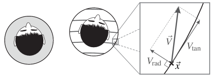
Figure 1: Radial and tangential component of the particle velocity vector defined on the circular contour around a local listening area.

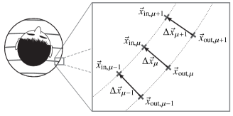
Figure 2: Pairs of control points located on the contour around a local listening area for JPVM+ such that the radial component of the particle velocity vector can be approximated.

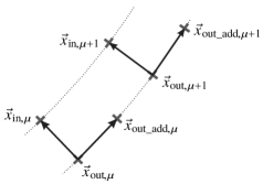
Figure 3: L-shaped groups of control points located on the contour around a local listening as required for the original version of JPVM buerger2015multi .

​-B Joint Optimization of Pressure and Particle Velocity

We now derive the optimization problem for the improved version of JPVM, referred to as JPVM+, where the individual steps of the derivation follow the same line as the ones presented in the original paper buerger2015multi . To formally describe the cost function for JPVM+, we first arrange the acoustic transfer functions from the $l$-th loudspeaker to all $M$ control points on each circle in column vectors $\mathbf{g}_{c,l}^{z}(\omega)=\left[G(\vec{x}_{c,1}^{z}|\vec{y}_{l},\omega),\ldots,G(\vec{x}_{c,M}^{z}|\vec{y}_{l},\omega)\right]^{\operatorname{T}}$, where the superscript $z\in\{\text{B},\text{D}\}$ indicates the bright or dark zone, and the subscript $c\in\{\text{in},\text{out}\}$ refers to the inner or outer circle of control points. Using this notation, the transfer functions from the entire set of loudspeakers to all control points can be conveniently captured in

$$\mathbf{G}(\omega)=\begin{bmatrix}\mathbf{g}_{\text{out},1}^{\text{B}}(\omega),\ldots,\mathbf{g}_{\text{out},{N_{\text{L}}}}^{\text{B}}(\omega)\\[3.0pt] \mathbf{g}_{\text{in},1}^{\text{B}}(\omega),\ldots,\mathbf{g}_{\text{in},{N_{\text{L}}}}^{\text{B}}(\omega)\\[3.0pt] \mathbf{g}_{\text{out},1}^{\text{D}}(\omega),\ldots,\mathbf{g}_{\text{out},{N_{\text{L}}}}^{\text{D}}(\omega)\\[3.0pt] \mathbf{g}_{\text{in},1}^{\text{D}}(\omega),\ldots,\mathbf{g}_{\text{in},{N_{\text{L}}}}^{\text{D}}(\omega)\\[3.0pt] \end{bmatrix},$$ (9)

such that the sound pressure at the control points can be compactly written as

$$\mathbf{p}(\omega)=\underbrace{\mathbf{G}(\omega)\mathbf{w}(\omega)}_{\mathbf{g}^{\text{p}}(\omega)}S(\omega),$$ (10)

with $\mathbf{g}^{\text{p}}$ representing the transfer function of the overall system w.r.t. the sound pressure.

As only the radial component of the particle velocity vector is considered here, which is motivated in Sec. IV, the original difference matrix buerger2015multi used for computing the corresponding pressure differences simplifies to

$$\mathbf{D}(\omega)=-\frac{1}{\mathrm{i}\omega\rho\Delta R}\left[\;\smash[b]{\underbrace{\begin{matrix}-\mathbf{I}&\mathbf{I}\\ \mathbf{0}&\mathbf{0}\\ \end{matrix}}_{\parbox{22.76228pt}{\scriptsize\centering bright zone\@add@centering}}}\right.\vphantom{\underbrace{\begin{matrix}-\mathbf{I}&\mathbf{I}\\ \mathbf{0}&\mathbf{0}\\ \end{matrix}}_{\parbox{22.76228pt}{\scriptsize\centering bright zone\@add@centering}}}\left.\smash[b]{\underbrace{\begin{matrix}\mathbf{0}&\mathbf{0}\\ -\mathbf{I}&\mathbf{I}\\ \end{matrix}}_{\parbox{22.76228pt}{\scriptsize\centering dark zone\@add@centering}}}\;\right]\vphantom{\underbrace{\begin{matrix}\mathbf{0}&\mathbf{0}\\ -\mathbf{I}&\mathbf{I}\\ \end{matrix}}_{\parbox{22.76228pt}{\scriptsize\centering dark zone\@add@centering}}}$$ (11)

where $\Delta R=\left\lVert\Delta\vec{x}_{\mu}\right\rVert_{2}\ \forall\mu$ represents the absolute difference between radii $R_{\text{in}}$ and $R_{\text{out}}$ of the inner and the outer circle of control points, respectively. Furthermore, $\mathbf{I}$ and $\mathbf{0}$ denote an identity and zero matrix, respectively, of dimensions $M\times M$. The resulting radial components of the particle velocity vector along the contours of the bright and dark zone are then given by

$$\mathbf{v}_{\text{rad}}(\omega)=\underbrace{\mathbf{D}(\omega)\mathbf{G}(\omega)\mathbf{w}(\omega)}_{\mathbf{g}^{\text{vel}}(\omega)}S(\omega),$$ (12)

where $\mathbf{g}^{\text{vel}}$ represents the transfer function of the overall system w.r.t. the radial component of the particle velocity vector.

Using  12 and  10, a weighted least squares optimization criterion for both quantities can be formulated,

$$\min\limits_{\mathbf{w}(\omega)}\left\{\kappa(\omega)\left\lVert\mathbf{G}(\omega)\mathbf{w}(\omega)-\mathbf{h}_{\text{des}}^{\text{p}}(\omega)\right\rVert_{2}^{2}\hskip 5.0pt+(1-\kappa(\omega))\left\lVert\mathbf{D}(\omega)\mathbf{G}(\omega)\mathbf{w}(\omega)-\mathbf{h}_{\text{des}}^{\text{vel}}(\omega)\right\rVert_{2}^{2}\right\},$$ (13)

where $\mathbf{h}_{\text{des}}^{\text{p}}$ and $\mathbf{h}_{\text{des}}^{\text{vel}}$ represent the desired pressure and velocity transfer functions, respectively, and $\kappa(\omega)\in[0,1]$ is used to adjust the relative weight of each quantity. Similar to the original JPVM approach buerger2015multi , the optimization problem  13 can be reformulated using stacked matrices such that a common least squares problem is obtained, which can then be solved in a closed form, e.g., using a Moore–Penrose pseudoinverse with Tikhonov regularization golub96matrix . For the sake of brevity, these steps are omitted here. Note that the cost function for JPVM+ does not contain the tangential component of the particle velocity vector implying that the optimization problem has a lower complexity compared to JPVM.

IV Analysis of the Impact of the Particle Velocity Vector Components on JPVM

In this section, we want to analyze how the individual components of the particle velocity vector affect the behavior and performance of JPVM. For this purpose, the sound pressure is formulated in the modal domain, where important fundamental relations are discussed in Sec. ​-A. Similar to the sound pressure, a modal representation of the radial and tangential component of the particle velocity vector is introduced in Sec. ​-B and Sec. ​-C, respectively. Finally, a representative example is given in Sec. ​-D which illustrates how well the different quantities on the contour are suited to control the sound field in the interior.

​-A Modal Representation of Sound Fields Evoked by Point Sources in a 2D Plane

The loudspeakers in this work are modeled as point sources, which is a simple yet reasonable approximation of real loudspeakers. This implies that, even though the previous considerations are limited to a 2D plane, the sound fields are in fact three-dimensional, where any point $\vec{x}$ in the 3D space can be addressed by its azimuth angle $\phi$, colatitude angle $\theta$, and radius $r$. It is well known that arbitrary 3D sound fields within a source-free region can be described as williams1999fourier

$$P(r,\theta,\phi,\omega)=\sum\limits_{n=0}^{\infty}\sum\limits_{m=-n}^{n}\alpha_{mn}(\omega)j_{n}(kr)Y_{n}^{m}(\theta,\phi),$$ (14)

where

$$Y_{n}^{m}(\theta,\phi)=\underbrace{\sqrt{\frac{(2n+1)}{4\pi}\frac{(n-\left\lvert m\right\rvert)!}{(n+\left\lvert m\right\rvert)!}}}_{b_{mn}}P_{n}^{\left\lvert m\right\rvert}(\cos\theta)\operatorname{e}^{+\mathrm{i}m\phi}$$ (15)

are the spherical harmonics of order $n$ and degree $m$, with $P_{n}^{m}$ being the associated Legendre functions, $j_{n}$ is the $n$-th order spherical Bessel function, and $\alpha_{mn}$ are the modal weights.

For a point source with frequency response $A(\omega)$ located at radius $r_{0}$ and direction ($\theta_{0},\phi_{0}$), the modal weights are given by colton2012inverse

$$\alpha_{mn}^{\text{PS}}(\omega)=-\mathrm{i}A(\omega)kh_{n}^{(2)}(kr_{0})b_{mn}P_{n}^{\left\lvert m\right\rvert}(\cos\theta_{0})\operatorname{e}^{-\mathrm{i}m\phi_{0}},$$ (16)

where $h_{n}^{(2)}$ denotes the $n$-th order spherical Hankel function of the second kind. Note that  14 with modal weights according to  16 and $A(\omega)=1\ \forall\omega$ is equivalent to the 3D Green’s function  1. As we assume in this work that the loudspeakers and observation points lie in the $x$-$y$ plane, i.e., $\theta_{0}=\pi/2$ and $\theta=\pi/2$, we omit the colatitude angles $\theta$ and $\theta_{0}$ in the notation for brevity. Using the above modal representation, the sound pressure evoked by a single loudspeaker, which is modeled as an ideal point source here, can be expressed as

$$P(r,\phi,\omega)=\sum\limits_{n=0}^{\infty}\sum\limits_{m=-n}^{n}\alpha_{mn}^{\text{PS}}(\omega)j_{n}(kr)b_{mn}P_{n}^{\left\lvert m\right\rvert}(1)\operatorname{e}^{+\mathrm{i}m\phi}.$$ (17)

On the other hand, the sound pressure at the circular contour around a local listening area can be represented by a Fourier series. More precisely, we express the sound pressure at the outer circle of control points with radius $R_{\text{out}}$ as

$$P(R_{\text{out}},\phi,\omega)=\sum\limits_{\mu=-\infty}^{\infty}a_{\mu}(R_{\text{out}},\omega)\operatorname{e}^{\mathrm{i}\mu\phi},$$ (18)

where $a_{\mu}$ are the Fourier coefficients. The coefficients $a_{\mu}$ obtained for a single point source can be computed by equating  18 with  17 and evaluating the inner product with the complex harmonics, i.e.,

$$a_{\mu}(R_{\text{out}},\omega)=\frac{1}{2\pi}\int\limits_{0}^{2\pi}\sum\limits_{n=0}^{\infty}\sum\limits_{m=-n}^{n}\alpha_{mn}^{\text{PS}}(\omega)j_{n}(kR_{\text{out}})b_{mn}P_{n}^{\left\lvert m\right\rvert}(1)\operatorname{e}^{+\mathrm{i}m\phi}\operatorname{e}^{-\mathrm{i}\mu\phi}\text{d}\phi.$$ (19)

Due to the orthogonality of complex harmonics, the integral may only be non-zero for $\mu=m$ such that the Fourier coefficients are given by

$$a_{m}(R_{\text{out}},\omega)=\sum\limits_{n=\left\lvert m\right\rvert}^{\infty}\alpha_{mn}^{\text{PS}}(\omega)\underbrace{j_{n}(kR_{\text{out}})b_{mn}P_{n}^{\left\lvert m\right\rvert}(1)}_{\gamma_{mn}(k,R_{\text{out}})}.$$ (20)

Note that the summation over $n$ in  20 must be limited to $n\geq\left\lvert m\right\rvert$, since $\left\lvert m\right\rvert$ of an associated Legendre function cannot be larger $n$. This is equivalent to the limitation of the sum over $m$ from $-n,\ldots,n$ in  14. From  20, it can be seen that a particular Fourier coefficient $a_{m}$ corresponds to a weighted sum of the modal weights $\alpha_{mn}^{\text{PS}}$ for a given degree $m$ and all orders $n$, where the individual weights are given by a set of scalar factors $\gamma_{mn}$. This set of frequency-dependent factors $\gamma_{mn}$ can be interpreted as a Multiple-Input Single-Output (MISO) system, which maps all modal weights for a particular index $m$ onto a Fourier coefficient representing a corresponding quantity on the contour (here: sound pressure), as illustrated in Fig. 4. Thus, a particular Fourier coefficient $a_{m}$ obtained at the output of such a MISO system describes how well the weighted sum of all modes of degree $m$ can be observed when evaluating the sound pressure on the contour. In case the mapping due to $\gamma_{mn}$ results in a very small absolute value $a_{m}$, a given set of modal weights $\alpha_{mn}^{\text{PS}}$ thus appears on the contour as strongly attenuated.

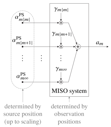
Figure 4: Schematic illustration of the mapping of the modal weights $\alpha_{mn}^{\text{PS}}$, with $n=\left\lvert m\right\rvert,\ldots,\infty$, onto the Fourier coefficients $a_{m}$ representing the sound pressure on the contour around a local listening area. For brevity, the frequency-dependency is omitted here.

To illustrate the mapping performed by  20, the Fourier coefficient $a_{0}$ is plotted in Fig. 5 for $R_{\text{out}}=0.3\,\mathrm{m}$ and a point source located at $r_{0}=2.5\,\mathrm{m}$, where the source direction $\phi_{0}$ is irrelevant here due to $m=0$. As expected, the magnitude of $a_{m}$ is strongly frequency-dependent, and the weighted sum of all modes for a given $m$ cannot be observed well at certain frequencies. Interestingly, the envelope/magnitude of $\alpha_{0}$ very closely follows the zeroth-order cylindrical Bessel function $J_{0}$ rather than the spherical Bessel function $j_{0}$, even though the sound field is resulting from a point source. This behavior cannot only be observed for the coefficient $a_{0}$, but for $a_{m}$ in general. It should be noted, however, that the cylindrical Bessel functions exhibit zero transitions, whereas the magnitude of $a_{m}$ does not take on the value zero for the corresponding arguments.

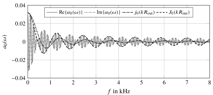
Figure 5: Fourier coefficient $a_{0}$ of the sound pressure $P$ at $R_{\text{out}}=0.3\,\mathrm{m}$ as resulting from a point source located at $r_{0}=2.5\,\mathrm{m}$ in the $x$-$y$ plane.

The previous considerations describe the mapping from given modal weights $\alpha_{mn}^{\text{PS}}$ onto the Fourier coefficients $a_{m}$ representing the sound pressure on the contour around a local listening area. If, on the other hand, the sound field shall be controlled by evoking the sound pressure on the contour, the inverse mapping comes into play. From a system-theoretical point of view, this may seem problematic, since it suggests the inversion of a MISO system. However, the factors $\gamma_{mn}$ of this MISO system only depend on the positions of the control points and are thus known. Furthermore, the modal coefficients $\alpha_{mn}^{\text{PS}}$ are dictated by the physics of a point source and its position. This implies that, for the given setup with a point source located in the $x$-$y$ plane, there is only a single possible set of modal coefficients (up to a scaling due to $A(\omega)$) for a given sound pressure on the contour. Only in case $a_{m}$ was equal to zero, infinitely many sets of modal coefficients would be possible, which is referred to as the nonuniqueness problem fazi2012nonuniqueness . Nevertheless, the inverse mapping may be ill-conditioned fazi2007ill and involve a strong amplification, such that low absolute values of the sound pressure on the contour may correspond to large values of the sound pressure in the interior of the local listening area. Accordingly, the sound pressure on the contour must then be evoked very precisely in order to reproduce the desired sound field properly, and even small errors on the contour may lead to a substantial deterioration in the interior. The observability of the modes on the contour can therefore be regarded as a robustness indicator: The larger the values of $a_{m}$ are, the less the sound field in the interior of the zone is affected by reproduction errors on the contour.

Similarly to the sound pressure itself, the radial and tangential pressure differences on the contours around the local listening areas may also be represented in terms of Fourier series, as shown below. The expressions thus obtained provide insights into the behavior of JPVM and serve as a basis for the modifications underlying the improved version JPVM+.

​-B The Radial Component of the Particle Velocity Vector

Analogously to the above, let us again consider a single loudspeaker located in the $x$-$y$ plane. Using the spherical harmonics representation of Eqs. 14, 15 and 16, the radial pressure difference in the numerator of  6 for a certain angle $\phi$ on the contour can be expressed as

$$\begin{split}\Delta P_{\text{rad}}(R_{\text{in}},R_{\text{out}},\phi,\omega)=&P(R_{\text{in}},\phi,\omega)-P(R_{\text{out}},\phi,\omega)\\ =&\sum\limits_{n=0}^{\infty}\sum\limits_{m=-n}^{n}\alpha_{mn}^{\text{PS}}(\omega)\underbrace{\left(j_{n}(kR_{\text{in}})-j_{n}(kR_{\text{out}})\right)b_{mn}P_{n}^{\left\lvert m\right\rvert}(1)}_{\gamma_{\text{rad},mn}(R_{\text{in}},R_{\text{out}},\omega)}\operatorname{e}^{\mathrm{i}m\phi}\\ =&\sum\limits_{m=-\infty}^{\infty}\underbrace{\sum\limits_{n=\left\lvert m\right\rvert}^{\infty}\alpha_{mn}^{\text{PS}}(\omega)\gamma_{\text{rad},mn}(R_{\text{in}},R_{\text{out}},\omega)}_{\Delta a_{\text{rad},m}(R_{\text{in}},R_{\text{out}},\omega)}\operatorname{e}^{\mathrm{i}m\phi},\end{split}$$ (21)

where the order of the summations over $m$ and $n$ is exchanged in the last step and the limits are adapted accordingly. Similarly to $\gamma_{mn}$ in  20, the set of frequency-dependent factors $\gamma_{\text{rad},mn}$ in  21 also describe a MISO system. The difference to  20 is that the modal weights $\alpha_{mn}^{\text{PS}}$ are now mapped onto Fourier coefficients $\Delta a_{\text{rad},m}$ which represent the radial pressure difference on the contour rather than the sound pressure itself. Accordingly, the output $\Delta a_{\text{rad},m}$ of the system describes how well the weighted sum of all modes of degree $m$ can be observed on the contour when evaluating the radial pressure difference. In turn, it also tells us how robustly a desired sound field can be reproduced by evoking the radial pressure difference on the contour. Before discussing the behavior of the radial pressure difference, we first want to also express the tangential pressure difference, which is also optimized in the original version of JPVM buerger2015multi , in the same way.

​-C The Tangential Component of the Particle Velocity Vector

Expressing the tangential pressure difference in the numerator of  8 by means of the spherical harmonics representation yields

$$\begin{split}\Delta P_{\text{tan}}(R_{\text{out}},\phi,\omega)=&P(R_{\text{out}},\phi+\Delta\phi,\omega)-P(R_{\text{out}},\phi,\omega)\\ =&\sum\limits_{n=0}^{\infty}\sum\limits_{m=-n}^{n}\alpha_{mn}^{\text{PS}}(\omega)\underbrace{j_{n}(kR_{\text{out}})b_{mn}P_{n}^{\left\lvert m\right\rvert}(1)\left(\operatorname{e}^{\mathrm{i}m\Delta\phi}-1\right)}_{\gamma_{\text{tan},mn}(R_{\text{out}},\Delta\phi,\omega)}\operatorname{e}^{\mathrm{i}m\phi}\\ =&\sum\limits_{m=-\infty}^{\infty}\underbrace{\sum\limits_{n=\left\lvert m\right\rvert}^{\infty}\alpha_{mn}^{\text{PS}}(\omega)\gamma_{\text{tan},mn}(R_{\text{out}},\Delta\phi,\omega)}_{\Delta a_{\text{tan},m}(R_{\text{out}},\Delta\phi,\omega)}\operatorname{e}^{\mathrm{i}m\phi},\end{split}$$ (22)

where $\Delta\phi$ denotes the angle between two neighboring control points on the circle with radius $R_{\text{out}}$. The frequency-dependent gain factors $\gamma_{\text{tan},mn}$ represent another MISO system, which maps the modal coefficients $\alpha_{mn}^{\text{PS}}$ onto Fourier coefficients $\Delta a_{\text{tan},m}$ representing the tangential pressure difference along the contour. Again, these coefficients indicate how well a sound field can be controlled by evoking the tangential pressure difference on the contour. It can be seen directly from  22 that the tangential pressure difference component $\Delta a_{\text{tan},m}$ is a scaled version of the sound pressure component $a_{m}$, where the scaling factor $\text{exp}\left(\mathrm{i}m\Delta\phi\right)-1$ is absolutely much smaller than one for small $\Delta\phi$ and low degrees $m$. This implies that the sound pressure itself can typically be better observed than the tangential pressure difference.

A more detailed discussion and comparison of the different mappings of modal coefficients due to $\gamma_{mn}$, $\gamma_{\text{rad},mn}$, and $\gamma_{\text{tan},mn}$ onto the corresponding Fourier coefficients representing the sound pressure on the contour, the radial pressure difference, and the tangential pressure difference, respectively, is provided below.

​-D Controllability of the Sound Pressure and its Radial and Tangential Difference

As an example, let us consider a point source located at $r_{0}=2.5\,\mathrm{m}$ and $\phi_{0}=\pi$, where the circles accommodating the control points are of radii $R_{\text{in}}=0.275\,\mathrm{m}$ and $R_{\text{out}}=0.3\,\mathrm{m}$, and the observation angle is $\phi=0^{\circ}$. The angular difference $\Delta\phi$ is chosen such that the absolute angular distance between two control points on the outer circle is identical to the absolute radial distance $\Delta R=2.5\,\mathrm{cm}$.

Figure 6 shows the resulting Fourier coefficients $a_{m}$, $\Delta a_{\text{rad},m}$, and $\Delta a_{\text{tan},m}$ for $m=1$, which represent the respective component of the sound pressure, the radial pressure difference, and the tangential pressure difference on the contour. It can be seen that sound pressure component $a_{1}$, whose magnitude behaves similarly as the magnitude of the Bessel function $J_{1}$, cannot be observed well on the contour for certain frequencies. Conversely, reproducing a sound field by controlling the sound pressure on the contour is prone to reproduction errors for these frequencies. Especially in a multizone scenario, reproduction errors are inevitably occurring as the optimization problem is typically ill-conditioned, such that a regularization is required in order to limit the gains of the loudspeaker prefilters. Therefore, a low performance must be expected for these frequencies.

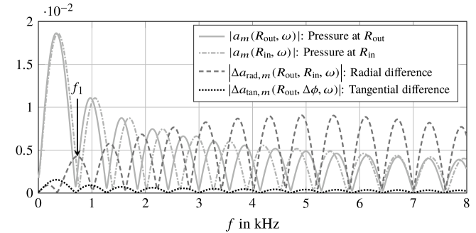
Figure 6: Magnitudes of the observed Fourier coefficients representing the sound pressure components for $m=1$ on the contour as well as the radial and tangential pressure differences.

A similar reasoning holds for the radial pressure difference $a_{\text{rad},m}$, which too exhibits low values at some frequencies, as can also be seen in Fig. 6 for $m=1$. However, the frequencies at which the local minima occur are shifted relative to the ones of the sound pressure itself. As a consequence, the radial pressure difference has generally large values if the pressure itself is low, and vice versa, such that at least one quantity can be used to robustly excite the sound field. Only for few frequencies beyond $5\,\mathrm{kHz}$, the local minima of the sound pressure component and the radial pressure difference lie closely together. It is worth noting here that the location of the local minima of the radial pressure difference can be controlled by the distance $\Delta R$ between the two circles of control points. If $\Delta R\rightarrow 0$, as an extreme case, the difference becomes proportional to the spatial derivative with its extremal values being at those frequencies where the magnitude of the sound pressure component has its steepest slope, i.e., in the vicinity of the local minima. Even though this may seem to be the best choice, the absolute values of the radial pressure difference $a_{\text{rad},m}$ would then be very small for all frequencies which again implies a low robustness against reproduction errors. Therefore, a compromise needs to be found between the absolute values of $a_{\text{rad},m}$ and the locations of the local minima by choosing proper values for $\Delta R$.

Finally, the magnitude of the Fourier coefficient $\Delta a_{\text{tan},m}$ describing the tangential pressure difference on the contour is also plotted in Fig. 6 for $m=1$. In contrast to the radial pressure difference, the tangential pressure difference defined in  22 typically is very small. The main reason for it is that the scaling factor $\text{exp}(\mathrm{i}m\Delta\phi)-1$ generally takes on very low absolute values, unless very high degrees $m$ or a large spacing $\Delta\phi$ are considered. Due to the fact that $\Delta\phi$ must be chosen sufficiently small in order to approximate the spatial derivative well, the scaling factor will be generally much smaller than one. The components $\Delta a_{\text{tan},m}$ representing the tangential pressure difference are therefore also much smaller than the components $a_{m}$ for the pressure itself. Moreover, the local minima of $\Delta a_{\text{tan},m}$ coincide with the local minima of $a_{m}$, such that an optimization of the tangential pressure difference does not provide any benefit over the sound pressure itself. In fact, evoking the tangential pressure difference may even degrade the reproduction performance, as shown in Sec. ​-C.

The analysis of the above example shows that it is beneficial to simultaneously control the sound pressure and the radial pressure difference. However, one may ask whether it is also sufficient to optimize only the sound pressure itself on two different radii, which should also (implicitly) control the radial pressure difference. The answer to that question can also be found in Fig. 6: For a frequency of $f_{1}=728\,\mathrm{Hz}$, as an example, the magnitude of $a_{1}$ representing sound pressure components for $m=1$ on the contour is equally small for both radii $R_{\text{in}}$ and $R_{\text{out}}$, i.e., a local minimum of $\max\left\{\left\lvert a_{1}(R_{\text{in}})\right\rvert,\left\lvert a_{1}(R_{\text{out}})\right\rvert\right\}$ is obtained. In fact, the PM approach exhibits a local performance minimum for frequencies around $f_{1}$, as will be shown by simulation results in Sec. ​-B. An explicit optimization of the radial pressure difference, on the other hand, does not suffer from this kind of performance drop, because the magnitude of the radial pressure difference component $\Delta a_{\text{rad},1}$ is significantly larger than the corresponding magnitudes of the individual sound pressure components for the considered frequency. In other words, the performance of the PM approach is dictated by two pressure components of the same magnitude, whereas the JPVM/JPVM+ approach can also exploit and optimize a quantity whose absolute value is significantly larger due to the phase differences between the individual pressure components. Therefore, an explicit optimization of the radial pressure difference is more robust to errors than an implicit optimization. Nevertheless, the optimization of the sound pressure $a_{m}$ on two circles with different radii rather than a single circle is still beneficial for frequencies where the absolute value of the radial pressure difference $a_{\text{rad},m}$ is smaller than the absolute values of both individual sound pressures themselves.

V Simulations

The reproduction performance of PM, JPVM, and JPVM+ is now evaluated for a simulated free-field environment, where the simulation setup and the utilized performance measures are explained in Sec. ​-A. Afterwards, a comparison of the three approaches is conducted in Sec. ​-B, before evaluation results are shown in Sec. ​-C which illustrate how the optimization of tangential pressure difference affects the reproduction performance. The impact of an explicit optimization of the radial component of the pressure difference is shown in Sec. ​-D by means of synthesized sound fields, which also demonstrate the broadband behavior of JPVM+. Finally, it is investigated in Sec. ​-E how inherent noise of the microphones, which are required to capture the Room Impulse Responses in practice, affects the reproduction performance.

​-A Simulation Setup

For a validation of the analytical findings presented above, we simulate a 70-element rectangular loudspeaker array of dimensions $3.95\,\mathrm{m}\times 3\,\mathrm{m}$ with an inter-element spacing of $9.6\,\mathrm{cm}$, where the loudspeakers are modeled as ideal point sources. This setup allows for a direct comparison with the results of the original JPVM paperbuerger2015multi . Two local listening areas are considered, whose centers are separated by a distance of $1\,\mathrm{m}$ along the $y$-axis and placed symmetrically w.r.t. the array center, as illustrated in Fig. 7. Each zone has a diameter of $0.6\,\mathrm{m}$ (implying that $R_{\text{out}}=0.3\,\mathrm{m}$), i.e., the edges of the bright zone $\mathcal{R}^{\text{B}}$ and the dark zone $\mathcal{R}^{\text{D}}$ are separated by $0.4\,\mathrm{m}$. The radius of the inner circle of control points is chosen as $R_{\text{in}}=0.275\,\mathrm{m}$, which amounts to a radial spacing of $\Delta R=2.5\,\mathrm{cm}$. To allow for a fair performance comparison, the number of utilized control points is identical for all approaches and amounts to 48 per zone. That is, 24 pairs of control points are uniformly distributed around each local listening area when applying the improved version JPVM+ and PM. In case of the original version of JPVM, which requires more control points on the outer circle, 16 L-shaped groups consisting of three control points each (cf. Fig. 3) are utilized for each zone, where both the radial and tangential spacing is $2.5\,\mathrm{cm}$. The relative weight $\kappa$ for the sound pressure and particle velocity in  13 is set to 0.04, and the minimization problem is solved using the Moore–Penrose pseudioinverse, where the regularization parameter is iteratively increased until the Loudspeaker Weight Energy (LWE) betlehem2012sound falls below the specified upper limit of $10/{N_{\text{L}}}$. As shown in the appendix, the chosen constraint on the LWE is comparable to a White Noise Gain (WNG) of $10\log_{10}(0.1{N_{\text{L}}})$. For comparison, a WNG of $10\log_{10}({N_{\text{L}}})$ corresponds to a delay-and-sum beamformer vantrees2004detection , which is the most robust beamformer and $10\,\mathrm{dB}$ larger than the one obtained here. The target sound field in the upper, bright zone is given by a plane wave originating from direction $\phi_{\text{src}}=-50^{\circ}$. This constitutes an especially difficult scenario as the effective distance between the zones as ‘observed’ from the source direction $\phi_{\text{src}}$ is close to zero. In other words, the acoustic energy needs to be focused very sharply and its level needs to rapidly drop in the lateral direction in order not to travel through the dark zone. Note that the plane wave front defining the target sound field in the bright zone does not have a magnitude of one, but it is scaled such that it corresponds to the magnitude which would be obtained with a point source located at a distance of $\bar{r}\approx 2\,\mathrm{m}$ from the center of $\mathcal{R}^{\text{B}}$, where $\bar{r}$ is the average distance from all loudspeakers to the zone center. If this scaling was not applied, the prefilters would need to compensate for the distance-dependent attenuation of the spherical waves emitted by the loudspeakers and, thus, have an inappropriately high energy. Furthermore, the above choice allows for directly relating the LWE to the WNG cox1986practical (see Appendix). All simulations are conducted using a sampling frequency of $f_{\text{s}}=8\,\mathrm{kHz}$, and a filter length $L=256$ is chosen for the loudspeaker prefilters.

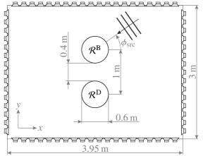
Figure 7: Schematic illustration of the reproduction setup with a plane-wave front originating from direction $\phi_{\text{src}}$ relative to the center of the bright zone $\mathcal{R}^{\text{B}}$.

As a first objective performance measure for the different reproduction algorithms, the Mean Squared Error (MSE) of the overall system transfer function w.r.t. the sound pressure is evaluated at ${N_{\text{grid}}}=441$ grid points in each zone,

$$\text{MSE}^{\left\{\text{B},\text{D}\right\}}(\omega)=\frac{1}{{N_{\text{grid}}}}\sum\limits_{q=1}^{{N_{\text{grid}}}}\left\lvert H_{\text{des}}\left(\vec{x}^{\left\{\text{B},\text{D}\right\}}_{q},\omega\right)-\mathbf{g}^{\operatorname{T}}\left(\vec{x}^{\left\{\text{B},\text{D}\right\}}_{q},\omega\right)\mathbf{w}(\omega)\right\rvert^{2},$$ (23)

where $\vec{x}^{\text{B}}_{q}\in\mathcal{R}^{\text{B}}$, $\vec{x}^{\text{D}}_{q}\in\mathcal{R}^{\text{D}}$, and the $x$- and $y$-spacing between the evaluation grid positions is $2\,\mathrm{cm}$. Furthermore, we evaluate the average level difference $\Delta L$ between the bright zone and the dark zone,

$$\Delta L(\omega)=10\log_{10}\left(\frac{E^{\text{B}}(\omega)}{E^{\text{D}}(\omega)}\right)\,\mathrm{dB},$$ (24)

where the average energies for $\mathcal{R}^{\text{B}}$ and $\mathcal{R}^{\text{D}}$ are computed as

$$E^{\left\{\text{B},\text{D}\right\}}(\omega)=\frac{1}{{N_{\text{grid}}}}\sum\limits_{q=1}^{{N_{\text{grid}}}}\left\lvert\mathbf{g}^{\operatorname{T}}\left(\vec{x}^{\left\{\text{B},\text{D}\right\}}_{q},\omega\right)\mathbf{w}(\omega)\right\rvert^{2}$$ (25)

at the same grid positions.

​-B Performance Comparison for PM, JPVM, and JPVM+

As a first investigation, we want to compare the performance obtained with PM poletti2008investigation , the original JPVM approach buerger2015multi , and the modified version JPVM+ presented here. As mentioned above, L-shaped groups of control points are used for JPVM, whereas the control points are arranged in pairs in case of PM and JPVM+. Even though this implies that the setup is not identical for all approaches, the number of utilized control points is the same such that the comparison is still fair.

The MSE inside the local listening areas obtained for the three approaches is shown as a function of frequency in Fig. 8(a). As can be seen, the performance of PM oscillates very strongly in the frequency range between about $250\,\mathrm{Hz}$ and $1250\,\mathrm{Hz}$, which is attributed to the ill-conditioning stemming from the low observability of certain modes at particular frequencies (cf. Sec. IV). For comparison purposes, the frequencies $f_{m}$ corresponding to the respective first local minimum of the magnitude of Fourier coefficient $a_{m}$ are indicated with arrows for $m=0,\ldots,3$. As can be seen, these frequencies match the local MSE maxima very well. When optimizing the entire particle velocity vector in addition to the sound pressure, as is the case in JPVM, the oscillation of the MSE curve can be significantly reduced, which implies a much more uniform performance and suggests less coloration of the perceived signal. However, the MSE can be reduced even further for almost all frequencies when utilizing JPVM+. This is due to the fact that the optimization of the tangential pressure difference in JPVM is very prone to (even tiny) errors, which cannot be avoided in practice. Especially in the bright zone, the performance towards higher frequencies clearly decreases for all approaches. Additional investigations showed that this can be mitigated by reducing the spacing between the loudspeakers, which leads to a lower spatial aliasing frequency, or by relaxing the constraint on the LWE. However, higher values of the LWE imply a lower robustness against errors typically occurring in practice, such as transducer noise, positioning errors, or variations of the properties of real loudspeakers.

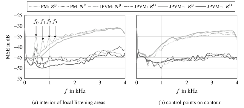
Figure 8: MSE inside (a) and at the control points around (b) the bright zone $\mathcal{R}^{\text{B}}$ and dark zone $\mathcal{R}^{\text{D}}$ for PM (dotted line), JPVM (dash-dotted line), and JPVM+ (solid line).

For completeness, the MSE for the control points themselves (i.e., the contour) is also shown in Fig. 8(b). Note that the MSE values are again computed according to  23. That is, the MSE only captures the sound pressure and not the particle velocity vector. As expected, the MSE is lowest in case of PM, where all degrees of freedom are used to optimize the sound pressure at the control points. Interestingly, the MSE at the control points has local minima at frequencies where the MSE inside the local listening area exhibits local maxima. This again indicates the problem that a low observability of the sound pressures on the contours, which form the basis for the optimization problem of PM, may lead to large reproduction errors in the interior of the zone. Evoking the sound pressure on the contour is thus not sufficient to infer the sound field inside the contour. In case of JPVM and JPVM+, the error of the sound pressure at the control points for frequencies below about $1.5\,\mathrm{kHz}$ is larger compared to PM, as some degrees of freedom are used to optimize the particle velocity (vector). Nevertheless, they result in a better performance inside the listening areas, as shown in Fig. 8(a).

Figure 8(a) may suggest that the benefit of JPVM+ over PM is rather low as the absolute MSE values in both zones are very low for all approaches. However, it is not sufficient to only assess the MSE, but it is also necessary to evaluate the achieved level difference $\Delta L$ between the two local listening areas, which is illustrated in Fig. 9. Again, the PM approach results in strong oscillations of the performance measure, where the level difference drops from $20\,\mathrm{dB}$ to almost $10\,\mathrm{dB}$ when increasing the frequency from $250\,\mathrm{Hz}$ to $450\,\mathrm{Hz}$. This implies that the acoustic scene to be synthesized in the bright zone does not leak into the dark zone equally strong for all frequencies, but certain frequencies produce more leakage than others. The level difference achieved with JPVM+, in contrast, is much more uniform and also clearly larger in the entire frequency range. This indicates that not only the overall energy in the dark zone is lower in case of JPVM+, but the arriving signals also have less coloration. The original JPVM approach ranges mostly between PM and JPVM+, and even though the curve is comparably smooth, the absolute level differences in certain frequency ranges are even lower than those of PM.

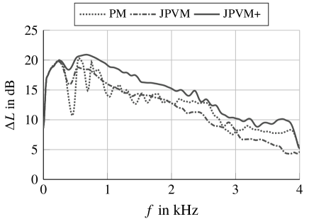
Figure 9: Level difference $\Delta L$ between the bright zone $\mathcal{R}^{\text{B}}$ and the dark zone $\mathcal{R}^{\text{D}}$ for PM (dotted line), JPVM (dash-dotted line), and JPVM+ (solid line).

​-C Impact of the Tangential Component of the Particle Velocity Vector

As the control points for JPVM and JPVM+ need to be arranged differently, we now want to evaluate a single setup and investigate in an isolated manner how the optimization of the tangential particle velocity vector component impairs the reproduction performance. For this purpose, we again consider the already evaluated setup for JPVM with 16 L-shaped groups of control points being distributed on the contour around each zone. The resulting frequency-dependent MSE obtained with JPVM is again shown in Fig. 10, which also contains the MSE obtained when excluding the tangential component of the particle velocity vector, i.e., when optimizing the sound pressure at all available control points and the radial component only. Note that the latter case does not correspond to JPVM+, as the control points are still arranged in L-shaped groups, and the number of control points on the outer circle is twice as large as for the inner circle. As can be seen in Fig. 10, the MSE is almost consistently lower if the tangential component is not optimized. Only for very few frequencies, a negligible performance degradation can be observed. These results confirm the insights obtained by the theoretical analysis presented in Sections ​-C and ​-D, and they show that the tangential component of the particle velocity vector should not be optimized, as doing so may generally reduce the reproduction performance. For completeness, the MSE obtained when excluding the radial component, i.e., when only optimizing the sound pressure at all available control points and the tangential component only, is also plotted in Fig. 10. This is to show that the MSE reduction obtained when neglecting the tangential component does not stem from the reduced complexity of the resulting optimization problem, and it furthermore confirms the efficacy of optimizing the radial component.

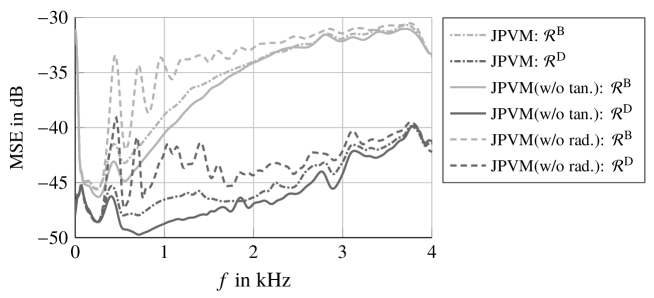
Figure 10: MSE inside the bright zone $\mathcal{R}^{\text{B}}$ and dark zone $\mathcal{R}^{\text{D}}$ for the original JPVM approach (dash-dotted line), the JPVM approach without the optimization of the tangential component of the particle velocity vector (solid line), and the JPVM approach without the optimization of the radial component of the particle velocity vector (dashed line).

​-D Impact of the Radial Component of the Particle Velocity Vector

In addition to the objective performance measure evaluated above, we now want to illustrate the benefit of explicitly optimizing the radial component of the particle velocity vector by means of visualizations of the sound fields synthesized by PM and JPVM+. Note that the illustrated sound fields are normalized in order to allow for a better assessment.

To demonstrate the broadband behavior of JPVM+, a von Hann impulse synthesized as a plane-wave front is shown in Fig. 11 for two time instants. The time instants are chosen such that a virtual plane perpendicular to the propagation direction of the wave front is at the center of the respective local listening area. It can be seen that the acoustic wave travels nicely around the lower, dark zone, where only the edge of the wave front leaks slightly into the interior of the zone (a). At the center of the upper, bright zone (b), a plane-wave front of desired orientation is synthesized. We do not show the corresponding plots of PM here, as the differences for these two time instants are rather hard to see when a short impulse is reproduced. Instead, the sound fields are illustrated for a frequency of $450\,\mathrm{Hz}$ and $700\,\mathrm{Hz}$ in Fig. 12. These frequencies are close to $f_{0}$ and $f_{1}$, which correspond to local minima of the magnitudes of the Fourier coefficients $a_{0}$ and $a_{1}$, respectively, representing the respective component of the sound pressure on the contour (see  20). Especially in the dark zone, it can be seen that the modes for $m=0$ (a) and $m=1$ (b) are erroneously excited in the interior of the zones when using PM. That is, a large sound energy is present in the dark zone at these frequencies, whereas the desired wave front in the bright zone is clearly distorted. The JPVM+ approach, on the other hand, only slightly excites the modes for $m=0$ in the dark zone (see Fig. 12(c)), and the modes for $m=1$ cannot be observed at all (see Fig. 12(d)). Similarly, the wave front in the bright zone is much less distorted for both frequencies.

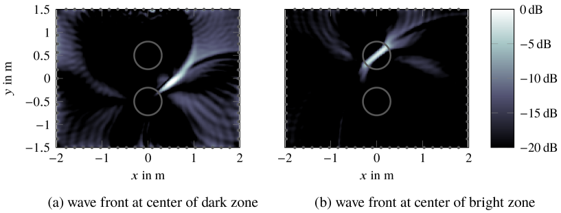
Figure 11: Reproduction of a plane-wave front for two different time instants using JPVM+.

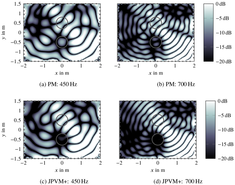
Figure 12: Reproduction of a plane-wave front of frequency $450\,\mathrm{Hz}$ and $700\,\mathrm{Hz}$ using PM and JPVM+.

​-E Sensor Noise

All previous simulations are based on the free-field assumption and it is assumed that the acoustic transfer functions are perfectly known. In practice, however, the reproduction system will typically be installed in a closed room and the sound waves emitted by the loudspeakers undergo reflections. In order to compensate for these undesired reflections, the acoustic properties of the room need to be captured, possibly in an adaptive manner. The topic of listening room equalization goetze2008multi ; schneider2012adaptive ; schneider2012iterative ; talagala2014efficient ; hofmann2016higher is not in the scope of this work and we would like to refer to literature here buerger2017multi . However, we still want to investigate how the utilization of real microphones for identifying the RIRs at the control points affects the reproduction performance. In addition to the inherent noise of microphones, RIR measurements typically also suffer from positioning errors and mismatches between the characteristics of the individual microphones. According to the work by Cox et al. cox1986practical and Teutsch teutsch2007modal , these imperfections have a similar effect as spatially white noise. To assess the impact on the performance of PM, JPVM, and JPVM+, we therefore add spatially uncorrelated white Gaussian noise sequences to the clean free-field RIRs corresponding to $\mathbf{G}$ in  13, where different Signal-to-Noise Ratios are considered. The free-field RIRs are of length 128 samples and the SNRs are determined based on the energies of the clean RIRs and the noise sequences. The broadband reproduction error (MSE) in the bright zone and the broadband level difference $\Delta L$ obtained from averaging  23 and  24, respectively, are listed in Table 1 for the three approaches. The table contains results for SNR values of $10\,\mathrm{dB}$, $20\,\mathrm{dB}$, $30\,\mathrm{dB}$, and $60\,\mathrm{dB}$, where only frequencies above $100\,\mathrm{Hz}$ are considered for evaluation. As expected, decreasing the SNR results in an increase of the MSE values and a reduction of the level difference. In case of PM, the MSE in the bright zone degrades by less than $0.5\,\mathrm{dB}$ when the SNR is reduced from $60\,\mathrm{dB}$ to $10\,\mathrm{dB}$. Due to the exploitation of the pressure differences, both JPVM and JPVM+ are more susceptible to sensor noise, where the MSE in the bright zone increases by more than $1\,\mathrm{dB}$ for both approaches. Nevertheless, the absolute MSE values are always lowest when utilizing JPVM+. The impact of sensor noise on the level difference $\Delta L$ is most pronounced in case of JPVM+, where a reduction of the SNR from $60\,\mathrm{dB}$ to $10\,\mathrm{dB}$ results in a degradation by more than $2.5\,\mathrm{dB}$. A slightly lower reduction of $\Delta L$ can be observed for JPVM, whereas the decrease for PM is below $1\,\mathrm{dB}$. However, JPVM+ achieves the highest absolute level differences throughout the entire SNR range. These results indicate that sensor noise should not be a severe problem in practice. It is worth noting that, albeit the average gain in level difference provided by JPVM+ relative to PM is only about $2\,\mathrm{dB}$ at most, the curves in Figures 8 and 9 indicate that JPVM+ introduces much less coloration, which is an important aspect when it comes the perceived reproduction quality.

Table 1: Impact of sensor noise on the reproduction accuracy in the bright zone (MSE) and the level difference $\Delta L$ between the bright zone and the dark zone when using PM, JPVM, and JPVM+.

	PM			JPVM			JPVM+
SNR in dB	$\Delta L$	MSE		$\Delta L$	MSE		$\Delta L$	MSE
10	12.3	-34.3		10.9	-33.7		12.7	-34.6
20	13.0	-34.7		12.7	-34.9		14.8	-35.8
30	13.1	-34.7		12.9	-35.2		15.2	-36.1
60	13.1	-34.8		13.0	-35.2		15.3	-36.2

VI Conclusion

In this paper, a recently proposed method for multizone sound reproduction, referred to as JPVM, is analyzed and further developed to yield the improved JPVM+ method. The core idea of JPVM is to independently control the sound field in different zones by jointly optimizing the sound pressure and particle velocity vector on the surrounding contours. The analysis of JPVM presented in this work utilizes spherical harmonics to describe the sound field and provides fundamental insights into its behavior. First of all, it illustrates that the optimization of the tangential component of the particle velocity vector is very prone to errors, and it may even degrade the reproduction performance. Therefore, JPVM+, an improved version of JPVM is proposed which only considers the radial component of the particle velocity vector. As a result, the computational complexity is reduced, while increasing the reproduction performance, as is verified by simulation results. The simulations also reveal that the error of the sound pressure on the contour is not a reliable measure for inferring the error in the interior. Finally, it is shown that sensor noise does not have a significant impact on the reproduction performance of JPVM+ despite relying on pressure differences.

Appendix: Relation between White Noise Gain and Loudspeaker Weight Energy

In this section, we want to relate the LWE betlehem2012sound to the WNG cox1986practical , which is a well-known and commonly used robustness measure in beamforming. The WNG is defined as the SNR obtained for a particular ‘target direction’ in the presence of spatially white transducer noise of unit variance. In the context of multizone sound rendering, not only the direction, but also the distance is crucial, such that the target direction becomes a ‘target position’. In fact, it is only meaningful to compute the WNG for target positions $\vec{x}^{\text{B}}$ in the bright zone $\mathcal{R}^{\text{B}}$, as the desired signal in the dark zone $\mathcal{R}^{\text{D}}$ is typically zero which, in the ideal case, would imply an SNR of $-\infty\,\mathrm{dB}$.

To establish a relation between the WNG and the LWE, let us consider the optimization problem for pressure matching  4 with an additional constraint on the LWE,

$$\min\limits_{\mathbf{w(\omega)}}\left\lVert\mathbf{G}(\omega)\mathbf{w(\omega)}-\mathbf{h}_{\text{des}}^{\text{p}}(\omega)\right\rVert_{2}^{2}\quad\text{s.~{}t.}\quad\left\lVert\mathbf{w}(\omega)\right\rVert_{2}^{2}\leq\alpha,$$ (26)

where $\alpha$ is the upper bound for the LWE. The target sound field in the bright zone is chosen as

$$H_{\text{des}}\left(\vec{x}^{\text{B}},\omega\right)=\frac{1}{4\pi\left\lVert\vec{y}-\vec{x}^{\text{B}}\right\rVert_{2}}\operatorname{e}^{-\mathrm{i}k\left\lVert\vec{y}-\vec{x}^{\text{B}}\right\rVert_{2}},$$ (27)

which corresponds to the sound pressure that would be obtained with a single loudspeaker located at position $\vec{y}$. For simplicity, we assume in the following that the bright zone is located at the center of a circular loudspeaker array of radius $r_{0}$. Furthermore, it is assumed that $\left\lVert\vec{y}\right\rVert_{2}=r_{0}$ and that the bright zone is sufficiently small relative to the array radius $r_{0}$, i.e., the distance-dependent attenuation of the spherical waves emitted by the loudspeakers is approximately identical for all $\vec{x}^{\text{B}}$. Given that the optimization problem in  26 is solved reasonably well, the overall transfer function of the reproduction system w.r.t. the sound pressure at the target positions in the bright zone may be approximated as

$$\mathbf{g}^{\operatorname{T}}\big{(}\vec{x}^{\text{B}},\omega\big{)}\mathbf{w}(\omega)\approx\frac{1}{4\pi r_{0}}\operatorname{e}^{-\mathrm{i}k\left\lVert\vec{y}-\vec{x}^{\text{B}}\right\rVert_{2}}.$$ (28)

Note that, due to the assumption that the zone size is small relative to $r_{0}$, the level within the bright zone is approximately constant.

To specify the WNG, we also need to determine the noise signal $N\big{(}\vec{x}^{\text{B}},\omega\big{)}$ at the target position $\vec{x}^{\text{B}}$ as resulting from spatially white transducer noise. Denoting the spatially white noise signal originating from the $l$-th loudspeaker as $N_{l}(\omega)$, $l=1,\ldots,{N_{\text{L}}}$, the resulting noise signal $N\big{(}\vec{x}^{\text{B}},\omega\big{)}$ is given by (cf.  2)

$$\begin{split}N\big{(}\vec{x}^{\text{B}},\omega\big{)}&=\sum\limits_{l=1}^{{N_{\text{L}}}}G\big{(}\vec{x}^{\text{B}}|\vec{y}_{l},\omega\big{)}W_{l}(\omega)N_{l}(\omega)\\ &=\mathbf{w}^{\operatorname{T}}(\omega)\mathbf{n}\big{(}\vec{x}^{\text{B}},\omega\big{)},\end{split}$$ (29)

where $\mathbf{n}\big{(}\vec{x}^{\text{B}},\omega\big{)}=\big{[}G\big{(}\vec{x}^{\text{B}}|\vec{y}_{1},\omega\big{)}N_{1}(\omega),\ldots,G\big{(}\vec{x}^{\text{B}}|\vec{y}_{N_{\text{L}}},\omega\big{)}N_{N_{\text{L}}}(\omega)\big{]}^{\operatorname{T}}$ is a vector capturing the contributions of each loudspeaker to the noise field at $\vec{x}^{\text{B}}$.

According to its definition, the WNG can be expressed as

$$\begin{split}\acs{WNG}\big{(}\vec{x}^{\text{B}},\omega\big{)}&=\frac{\left\lvert\mathbf{g}^{\operatorname{T}}\big{(}\vec{x}^{\text{B}},\omega\big{)}\mathbf{w(\omega)}\right\rvert^{2}}{\mathcal{E}\left\{N\big{(}\vec{x}^{\text{B}},\omega\big{)}N^{*}\big{(}\vec{x}^{\text{B}},\omega\big{)}\right\}}\\ &\approx\frac{\frac{1}{(4\pi r_{0})^{2}}}{\mathbf{w}^{\operatorname{T}}(\omega)\underbrace{\mathcal{E}\left\{\mathbf{n}\big{(}\vec{x}^{\text{B}},\omega\big{)}\mathbf{n}^{\operatorname{H}}\big{(}\vec{x}^{\text{B}},\omega\big{)}\right\}}_{\mathbf{R}(\vec{x}^{\text{B}},\omega)}\mathbf{w}^{*}(\omega)},\end{split}$$ (30)

where $\mathcal{E}\left\{\cdot\right\}$ is the expectation operator and the superscript $(\cdot)^{*}$ denotes complex conjugation. As the noise signals $N_{l}$ are spatially white, the correlation matrix $\mathbf{R}$ is diagonal and contains the squared magnitudes of the individual Green’s functions. Due to the assumption that these magnitudes are approximately equal for all target positions, the correlation matrix can be approximated as

$$\mathbf{R}(\vec{x}^{\text{B}},\omega)\approx\frac{1}{(4\pi r_{0})^{2}}\mathbf{I}_{N_{\text{L}}},$$ (31)

with $\mathbf{I}_{N_{\text{L}}}$ being an identity matrix of dimensions ${N_{\text{L}}}\times{N_{\text{L}}}$. Inserting  31 into  30 finally yields

$$\acs{WNG}\big{(}\vec{x}^{\text{B}},\omega\big{)}\approx\frac{\frac{1}{(4\pi r_{0})^{2}}}{\frac{1}{(4\pi r_{0})^{2}}\mathbf{w}^{\operatorname{T}}(\omega)\mathbf{w}^{*}(\omega)}=\frac{1}{\left\lVert\mathbf{w}(\omega)\right\rVert_{2}^{2}}.$$ (32)

That is, the WNG can be approximated by the inverse of the LWE. Note that  32 is only valid if the target sound field for the bright zone is specified such that the distance-dependent attenuation resulting from the Green’s functions is considered. If the target sound field in  27 was defined with a magnitude of one, the WNG in  32 would be increased by a factor of $(4\pi r_{0})^{2}$. It shall finally be noted that, even though the distances between all loudspeakers and target positions are not identical in practice,  32 can still be used to obtain an approximate relation between the WNG and the LWE.

References

- (1) A. J. Berkhout, D. de Vries, and P. Vogel, “Acoustic control by wave field synthesis,” J. Acoust. Soc. Am. (JASA), vol. 93, no. 5, pp. 2764–2778, 1993.
- (2) S. Spors, R. Rabenstein, and J. Ahrens, “The Theory of Wave Field Synthesis Revisited,” in 124th Audio Eng. Soc. (AES) Conv., (Amsterdam), May 2008. Paper Number: 7358.
- (3) J. Ahrens, R. Rabenstein, and S. Spors, “Sound field synthesis for audio presentation,” Acoust. Today, vol. 10, no. 2, pp. 15–25, 2014.
- (4) M. A. Gerzon, “Ambisonics in multichannel broadcasting and video,” J. Audio Eng. Soc. (JAES), vol. 33, no. 11, pp. 859–871, 1985.
- (5) D. B. Ward and T. D. Abhayapala, “Reproduction of a plane-wave sound field using an array of loudspeakers,” IEEE Trans. Speech Audio Process., vol. 9, pp. 697–707, Sep 2001.
- (6) J. Ahrens and S. Spors, “Analytical driving functions for higher order ambisonics,” in Proc. IEEE Int. Conf. Acoustics, Speech, Signal Process. (ICASSP), pp. 373–376, IEEE, 2008.
- (7) J.-W. Choi and Y.-H. Kim, “Generation of an acoustically bright zone with an illuminated region using multiple sources,” J. Acoust. Soc. Am. (JASA), vol. 111, no. 4, pp. 1695–1700, 2002.
- (8) M. Poletti, “An investigation of 2-D multizone surround sound systems,” in Proc. 125th Audio Eng. Soc. (AES) Conv., Oct. 2008.
- (9) M. Shin, S. Q. Lee, F. M. Fazi, P. A. Nelson, D. Kim, S. Wang, K. H. Park, and J. Seo, “Maximization of acoustic energy difference between two spaces,” J. Acoust. Soc. Am. (JASA), vol. 128, no. 1, pp. 121–131, 2010.
- (10) J. Ahrens and S. Spors, “An analytical approach to local sound field synthesis using linear arrays of loudspeakers,” in Proc. IEEE Int. Conf. Acoustics, Speech, Signal Process. (ICASSP), pp. 65–68, IEEE, May 2011.
- (11) S. Spors and J. Ahrens, “Local sound field synthesis by virtual secondary sources,” in Proc. 40th Audio Eng. Soc. (AES) Conf.: Spatial Audio—Sense the Sound of Space, pp. 6–3, 2010.
- (12) Y. J. Wu and T. D. Abhayapala, “Spatial multizone soundfield reproduction: Theory and design,” IEEE Trans. Audio, Speech, Language Process., vol. 19, no. 6, pp. 1711–1720, 2011.
- (13) W. Jin, W. B. Kleijn, and D. Virette, “Multizone soundfield reproduction using orthogonal basis expansion,” in Proc. IEEE Int. Conf. Acoustics, Speech, Signal Process. (ICASSP), pp. 311–315, IEEE, 2013.
- (14) N. Radmanesh and I. S. Burnett, “Generation of isolated wideband sound fields using a combined two-stage lasso-ls algorithm,” IEEE Trans. Audio, Speech, Language Process., vol. 21, pp. 378–387, Feb. 2013.
- (15) P. Coleman, P. Jackson, M. Olik, and J. A. Pedersen, “Optimizing the planarity of sound zones,” in Proc. 52nd Audio Eng. Soc. (AES) Conf.: Sound Field Control—Engineering and Perception, 2013.
- (16) K. Helwani, S. Spors, and H. Buchner, “The synthesis of sound figures,” Multidimensional Systems and Signal Processing, vol. 25, no. 2, pp. 379–403, 2014.
- (17) W. Jin and W. B. Kleijn, “Multizone soundfield reproduction in reverberant rooms using compressed sensing techniques,” in Proc. IEEE Int. Conf. Acoustics, Speech, Signal Process. (ICASSP), pp. 4728–4732, IEEE, 2014.
- (18) Y. Cai, M. Wu, and J. Yang, “Sound reproduction in personal audio systems using the least-squares approach with acoustic contrast control constraint,” J. Acoust. Soc. Am. (JASA), vol. 135, no. 2, pp. 734–741, 2014.
- (19) M. A. Poletti and F. M. Fazi, “An approach to generating two zones of silence with application to personal sound systems,” J. Acoust. Soc. Am. (JASA), vol. 137, no. 2, pp. 598–605, 2015.
- (20) T. Betlehem, W. Zhang, M. A. Poletti, and T. D. Abhayapala, “Personal Sound Zones: Delivering interface-free audio to multiple listeners,” IEEE Signal Proc. Mag., vol. 32, pp. 81–91, March 2015.
- (21) M. Buerger, C. Hofmann, and W. Kellermann, “The Impact of Loudspeaker Array Imperfections and Reverberation on the Performance of a Multizone Sound Field Synthesis System,” in Proc. 3rd Int. Conf. Spatial Audio (ICSA), Sept. 2015.
- (22) M. Buerger, R. Maas, H. W. Löllmann, and W. Kellermann, “Multizone sound field synthesis based on the joint optimization of the sound pressure and particle velocity vector on closed contours,” in Proc. IEEE Workshop Applications Signal Process. to Audio, Acoustics (WASPAA), Oct. 2015.
- (23) M. A. Poletti and F. M. Fazi, “Generation of half-space sound fields with application to personal sound systems,” J. Acoust. Soc. Am. (JASA), vol. 139, no. 3, pp. 1294–1302, 2016.
- (24) F. Winter, N. Hahn, and S. Spors, “Time-domain realisation of model-based rendering for 2.5 d local wave field synthesis using spatial bandwidth-limitation,” in Proc. 25th Eur. Signal Process. Conf. (EUSIPCO), pp. 688–692, IEEE, 2017.
- (25) N. Hahn, F. Winter, and S. Spors, “Synthesis of a spatially band-limited plane wave in the time-domain using wave field synthesis,” in Proc. 25th Eur. Signal Process. Conf. (EUSIPCO), pp. 673–677, IEEE, 2017.
- (26) S. Spors, J. Ahrens, and K. Helwani, “Local sound field synthesis by virtual acoustic scattering and time-reversal,” in Proc. 131st Audio Eng. Soc. (AES) Conv., Oct 2011.
- (27) E. G. Williams, Fourier Acoustics: Sound Radiation and Nearfield Acoustical Holography. Academic Press, 1999.
- (28) G. H. Golub and C. F. V. Loan, Matrix Computations. Johns Hopkins University Press, third ed., 1996.
- (29) T. Betlehem and C. Withers, “Sound field reproduction with energy constraint on loudspeaker weights,” IEEE Trans. Audio, Speech, Language Process., vol. 20, pp. 2388–2392, Oct. 2012.
- (30) G. N. Lilis and D. Angelosante, “Sound field reproduction using the lasso,” IEEE Trans. Audio, Speech, Language Process., vol. 11, pp. 1902–1912, Nov. 2010.
- (31) L. L. Beranek, Acoustics. McGraw-Hill, 1954.
- (32) P. G. Craven and M. A. Gerzon, “Coincident microphone simulation covering three dimensional space and yielding various directional outputs,” Aug 1977. US Patent 4,042,779.
- (33) E. Benjamin and T. Chen, “The Native B-Format Microphone,” in Proc. 119th Audio Eng. Soc. (AES) Conv., Oct 2005.
- (34) H. Teutsch and G. W. Elko, “First-and second-order adaptive differential microphone arrays,” in Proc. Int. Workshop Acoustic Echo Noise Control (IWAENC), pp. 35–38, 2001.
- (35) D. Colton and R. Kress, Inverse Acoustic and Electromagnetic Scattering Theory. Springer, 2012.
- (36) F. M. Fazi and P. A. Nelson, “Nonuniqueness of the solution of the sound field reproduction problem with boundary pressure control,” Acta Acustica united with Acustica, vol. 98, no. 1, pp. 1–14, 2012.
- (37) F. M. Fazi and P. A. Nelson, “The ill-conditioning problem in sound field reconstruction,” in Proc. 123rd Audio Eng. Soc. (AES) Conv., Oct 2007.
- (38) H. L. V. Trees, Detection, Estimation, and Modulation Theory, Optimum Array Processing (Part IV). John Wiley & Sons, 2002.
- (39) H. Cox, R. M. Zeskind, and T. Kooij, “Practical supergain,” IEEE Trans. Acoust., Speech, Signal Process., vol. 34, no. 3, pp. 393–398, 1986.
- (40) S. Goetze, M. Kallinger, A. Mertins, and K. D. Kammeyer, “Multi-channel listening-room compensation using a decoupled filtered-x lms algorithm,” in Proc. 42nd Asilomar Conf. Signals, Syst., Comput., pp. 811–815, Oct 2008.
- (41) M. Schneider and W. Kellermann, “Adaptive listening room equalization using a scalable filtering structure in thewave domain,” in Proc. IEEE Int. Conf. Acoustics, Speech, Signal Process. (ICASSP), pp. 13–16, March 2012.
- (42) M. Schneider and W. Kellermann, “Iterative dft-domain inverse filter determination for adaptive listening room equalization,” in Proc. Int. Workshop Acoustic Echo Noise Control (IWAENC), pp. 1–4, Sept 2012.
- (43) D. S. Talagala, W. Zhang, and T. D. Abhayapala, “Efficient multi-channel adaptive room compensation for spatial soundfield reproduction using a modal decomposition,” IEEE Trans. Audio, Speech, Language Process., vol. 22, pp. 1522–1532, Oct 2014.
- (44) C. Hofmann, M. Guenther, M. Buerger, and W. Kellermann, “Higher-order listening room compensation with additive compensation signals,” in Proc. IEEE Int. Conf. Acoustics, Speech, Signal Process. (ICASSP), March 2016.
- (45) M. Buerger, C. Hofmann, C. Frankenbach, and W. Kellermann, “Multizone sound reproduction in reverberant environments using an iterative least-squares filter design method with a spatiotemporal weighting function,” in Proc. IEEE Workshop Applications Signal Process. to Audio, Acoustics (WASPAA), Oct. 2017.
- (46) H. Teutsch, Modal Array Signal Processing: Principles and Applications of Acoustic Wavefield Decomposition (Lecture Notes in Control and Information Sciences). Springer, 2007.