New entropic inequalities for qubit and unimodal Gaussian states

Abstract

The Tsallis relative entropy $S_{q}(\hat{\rho},\hat{\sigma})$ measures the distance between two arbitrary density matrices $\hat{\rho}$ and $\hat{\sigma}$. In this work the approximation to this quantity when $q=1+\delta$ ($\delta\ll 1$) is obtained. It is shown that the resulting series is equal to the von Neumann relative entropy when $\delta=0$. Analyzing the von Neumann relative entropy for arbitrary $\hat{\rho}$ and a thermal equilibrium state $\hat{\sigma}=e^{-\beta\hat{H}}/{\rm Tr}(e^{-\beta\hat{H}})$ is possible to define a new inequality relating the energy, the entropy, and the partition function of the system. From this inequality, a parameter that measures the distance between the two states is defined. This distance is calculated for a general qubit system and for an arbitrary unimodal Gaussian state. In the qubit case, the dependence on the purity of the system is studied for $T\geq 0$ and also for $T<0$. In the Gaussian case, the general partition function given a unimodal quadratic Hamiltonian is calculated and the comparison of the thermal light state as a thermal equilibrium state of the parametric amplifier is presented.

1 Introduction

The quantum aspects of thermodynamics have been subjects of intense studies in recent review articles; see, e.g., [1, 2]. There are many topics relating quantum information theory and thermodynamics since the Maxwell’s demon and the Landauer principle [3, 4] to entanglement in many-body systems [5]. In particular, how concepts and techniques from quantum mechanics or quantum information theory have been applied to thermodynamics [6] and inversely how concepts from thermodynamics are applied in the context of quantum information [7, 8, 9, 10].

The importance of the study of classical and quantum entropies as the ones defined by von Neumann [11] and Tsallis [12] for quantum information systems has been increasing in the last decade. In particular, new entropic inequalities are used to characterize quantum correlations of qudit systems [13]. They have lead to nonlinear relations between unitary matrices which have been checked in experiments of superconducting qudits [14, 15, 16].

The relative entropy [17] ($\textrm{Tr}\,(\hat{\rho}\ln\hat{\rho}-\hat{\rho}\ln\hat{\sigma})\geq 0$), has been used to describe finite systems approaching thermal equilibrium [18]; in those systems this quantity can be interpreted as information needed to change an arbitrary density matrix $\hat{\rho}$ to the thermal equilibrium $\hat{\sigma}$ [6].

In the previous work [19], it was found that the sum of the dimensionless energy $E(\hat{\rho},\hat{H})={\rm Tr}(\hat{\rho}\hat{H})$ and entropy $S(\hat{\rho})=-{\rm Tr}(\hat{\rho}\ln\hat{\rho})$ of the system is bounded by $\ln Z(\beta=-1,\hat{H})$, where the partition function $Z(\beta,\hat{H})={\rm Tr}(e^{-\beta\hat{H}})$ at $\beta=-1$ determines the value of the bound. As it was shown in [13], the sum of the energy and the entropy equals to the bound only if the density operator $\hat{\rho}$ of the system equals to the thermal equilibrium state at temperature value $T=-1$.

The aim of this work is to study the distance between and arbitrary density matrix and a state approaching thermal equilibrium. In order to do this, a new quantum inequality relating the free energy ($F(\hat{\rho},\hat{H},T)=-T\ln(Z(\beta,\hat{H}))$) of an arbitrary system with the corresponding partition function is obtained. We apply the inequality to a spin-1/2 state and also for an unimodal Gaussian state. We show that the bound in this inequality is determined by the thermal equilibrium state (TES) of the system and thus a parameter for the distance can be defined.

2 Tsallis relative entropy

The Tsallis relative entropy introduced in [20] and expressed as

$$S_{q}(\hat{\rho},\hat{\sigma})=\frac{1}{1-q}(1-{\rm Tr}(\hat{\rho}^{q}\hat{\sigma}^{1-q}))$$ (1)

measures the distance between the density matrices $\hat{\rho}$ and $\hat{\sigma}$. This quantity is zero iff the two are equal and greater than zero in other case. When $q\rightarrow 1$ this expression corresponds to the von Neumann relative entropy. If the parameter $q$ approach $1$ ($q=1+\delta$, $\delta>0$, $\delta\ll 1$), Eq. (1) can be written as a Taylor series of $\delta$ as follows:

$$S_{1+\delta}(\hat{\rho},\hat{\sigma}) = {\rm Tr}(\hat{\rho}(\ln\hat{\rho}-\ln\hat{\sigma}))+\frac{1}{2!}{\rm Tr}(\hat{\rho}(\ln\hat{\rho}-\ln\hat{\sigma})^{2})\delta+$$ (2)

$$+ \frac{1}{3!}({\rm Tr}(\hat{\rho}(\ln\hat{\rho}-\ln\hat{\sigma})^{3}+{\rm Tr}(\hat{\rho}(\ln\hat{\rho}\ln\hat{\sigma}-\ln\hat{\sigma}\ln\hat{\rho})\ln\hat{\sigma})))\delta^{2}+\mathcal{O}(\delta^{3})\,,$$

this expression can be checked using the expansion $\hat{\rho}^{q}=e^{q\ln\hat{\rho}}={\bf 1}+q\ln\hat{\rho}+q^{2}\ln^{2}\hat{\rho}/2!+\cdots$ and an analogous expression for $\hat{\sigma}$. Using the relative entropy between two states ($\hat{\rho}$ and $\hat{\sigma}$), where $\hat{\sigma}$ is a thermal equilibrium state, it is possible to show the relation between the energy, the entropy and the partition function. If the state $\hat{\sigma}$ corresponds to a mixed state dependent on a parameter $T$ (which it may or may not be related with the temperature of the system), in the form of

$$\hat{\sigma}=\frac{e^{-\beta\hat{H}}}{\textrm{Tr}(e^{-\beta\hat{H}})}\,,$$ (3)

then the positivity of the relative entropy defines an inequality relation between the entropy, energy and the normalization factor of $\hat{\sigma}$: Tr$(e^{-\beta\hat{H}})$. This relation for $T>0$ has the following form:

$$E(\hat{\rho},\hat{H})-TS(\hat{\rho})\geq-T\ln(Z(\beta,\hat{H}))\,.$$

This inequality must hold for any temperature $T$ for a fixed Hamiltonian. Defining the parameter $\Delta$ as

$$\Delta=E(\hat{\rho},\hat{H})-TS(\hat{\rho})+T\ln(Z(\beta,\hat{H}))\geq 0\,,$$ (4)

then the difference between any state and a TES can be evaluated.

In this work, the study of the $\Delta$ parameter is presented for an arbitrary qubit system and a general unimodal Gaussian state.

3 Qubit system

In a previous work [19], the entropy–energy relation for extremal density matrices describing qudit states was analyzed. In this section, a generalization of this relation is obtained for any qubit system.

The most general density matrix for a qubit system is parametrized by the Bloch vector $\mathbf{p}=(p_{x},p_{y},p_{z})$, where each component is given by the mean value of the Pauli matrices in a system described by the density matrix $\hat{\rho}$, i.e., $p_{x}={\rm Tr}(\hat{\rho}\,\hat{\sigma}_{x})$, $p_{y}={\rm Tr}(\hat{\rho}\,\hat{\sigma}_{y})$, and $p_{z}={\rm Tr}(\hat{\rho}\,\hat{\sigma}_{z})$. In this case, the density matrix $\hat{\rho}$ is given by the expression

$$\hat{\rho}=\frac{1}{2}\left(\begin{array}[]{cc}1+p_{z}&p_{x}-ip_{y}\\ p_{x}+ip_{y}&1-p_{z}\end{array}\right)\,.$$ (5)

In order to guaranty the positivity of the density matrix, the norm of its Bloch vector must be bounded $0\leq|\mathbf{p}|\leq 1$; on the other hand, this norm also fixes the purity of the state $|\mathbf{p}|=\sqrt{2\,{\rm Tr}(\hat{\rho}^{2})-1}$, if $|\mathbf{p}|=1$ the state is pure and in other case the state is mixed. Also if $|\mathbf{p}|=0$, the density matrix corresponds to the most mixed state.

In an analogous way, the Hamiltonian can be expressed in terms of its own Bloch vector $\mathbf{h}=(h_{1},h_{2},h_{3})$ as

$$\hat{H}=\frac{1}{2}\left(\begin{array}[]{cc}h_{0}+h_{3}&h_{1}-ih_{2}\\ h_{1}+ih_{2}&h_{0}-h_{3}\end{array}\right)\,,$$ (6)

where $h_{0}={\rm Tr}(\hat{H})$.

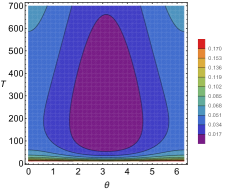
(a) (b)

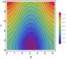
Figure 1: (a) Contour plots of the $\Delta$ parameter as a function of the $\theta$ angle for $T>0$ in a qubit system with $|\mathbf{p}|=0.01$ and $|\mathbf{h}|=\sqrt{14}$. (b) $|\mathbf{p}|=0.99$ .

In the most general case, the mean value of the energy, the entropy and the partition function of the system are given by the following

$$\langle\hat{H}\rangle=\frac{1}{2}(h_{0}+\mathbf{p}\cdot\mathbf{h}),\quad S=-\frac{1}{2}\{(1-|\mathbf{p}|)\ln(1-|\mathbf{p}|)+(1+|\mathbf{p}|)\ln(1+|\mathbf{p}|)\},$$

$$Z(\beta,\hat{H})=e^{-\beta h_{0}/2}\cosh(\beta|\mathbf{h}|/2)\,.$$ (7)

One can see that $\hat{\rho}$ corresponds to a thermal equilibrium state ($\Delta=0$), when its Bloch vector and the Bloch vector of the Hamiltonian follow the relation

$$\mathbf{p}=-\frac{\mathbf{h}}{|\mathbf{h}|}\tanh\left(\frac{\beta|\mathbf{h}|}{2}\right)\,,$$ (8)

this is when the Bloch vectors are antiparallel and $T=|\mathbf{h}|/(2\,{\rm arctanh}|\mathbf{p}|)$. In fig. (1a), one can see the dependence of the $\Delta$ parameter as a function of $\theta$ and $T$ for given $|\mathbf{p}|=0.01$ and $|\mathbf{h}|=\sqrt{14}$; in this case, $\Delta=0$ for $T\approx 187$. A small $|\mathbf{p}|$ indicates a state near the most mixed state (${\rm Tr}(\hat{\rho}^{2})=1/2$). In fig. (1b), the plots for $|\mathbf{p}|=0.99$ (almost a pure state) can be seen, in that case $\Delta=0$ for $T\approx 0.71$.

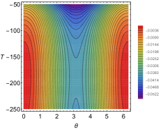
(a) (b)

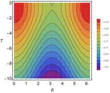
Figure 2: (a) Contour plots of the $\Delta$ parameter as a function of the $\theta$ angle for $T<0$ in a qubit system with $|\mathbf{p}|=0.01$ and $|\mathbf{h}|=\sqrt{14}$. (b) $|\mathbf{p}|=0.99$ .

It is possible to do the same analysis for $T<0$; in that case, the parameter $\Delta$ of Eq.(4) must be negative. The state $\hat{\rho}$ is a thermal equilibrium state when $\mathbf{p}$ and $\mathbf{h}$ are parallel for $T=-|\mathbf{h}|/(2\,{\rm arctanh}|\mathbf{p}|)$. The corresponding plots of this parameter are presented in fig. (2a) for an almost most mixed state ($|\mathbf{p}|=0.01$) and in fig. (2b) for an almost pure state ($|\mathbf{p}|=0.99$). In the case of the mixed state, $\Delta=0$ for $T\approx-187$, for $|\mathbf{p}|=0.99$ (almost pure state) $\Delta=0$ for $T\approx-0.71$.

4 Single-mode Gaussian states as thermal equilibrium states

In recent years, the Gaussian states have become very important due to their use in quantum information theory [21, 22]. In this section, we study the parameter $\Delta$ for a general unimodal Gaussian state. The most general unimodal Gaussian state (GS) is described by the density matrix

$$\hat{\rho}(q^{\prime},q)=\mathcal{N}e^{-a_{1}q^{2}-a_{1}^{*}q^{\prime 2}+a_{2}qq^{\prime}+b_{1}q+b_{1}^{*}q^{\prime}},$$

$$\mathcal{N}=\sqrt{\frac{a_{1}+a_{1}^{*}-a_{2}}{\pi}}\exp\left(\frac{-(b_{1}+b_{1}^{*})^{2}}{4(a_{1}+a_{1}^{*}-a_{2})}\right)\,,$$ (9)

where the normalization condition (${\rm Tr}(\hat{\rho})=1$) implies that parameter $a_{2}\in\mathbb{R}$ and $2\textrm{Re}(a_{1})>a_{2}$. The coherent state, the squeezed vacuum state and the thermal light state are examples of Gaussian states. The properties of these states are determined by the covariance matrix of the system $\boldsymbol{\sigma}$ and the mean values in the quadrature components ($\hat{p}$, $\hat{q}$). For the general case of Eq. (9), the covariance matrix is

$$\boldsymbol{\sigma}=\frac{1}{2(a_{1}+a_{1}^{*}-a_{2})}\left(\begin{array}[]{cc}4|a_{1}|^{2}-a_{2}^{2}&i(a_{1}^{*}-a_{1})\\ i(a_{1}^{*}-a_{1})&1\end{array}\right),$$ (10)

while the mean values are

$$\langle\hat{p}\rangle=\frac{a_{2}\,{\rm Im(b_{1})}-2\,{\rm Im}(a_{1}^{*}b_{1})}{2(a_{1}+a_{1}^{*}-a_{2})},\ \ \langle\hat{q}\rangle=\frac{b_{1}+b_{1}^{*}}{2(a_{1}+a_{1}^{*}-a_{2})}\,.$$ (11)

4.1 Quadratic Hamiltonian

It can be seen that a state of the form $e^{-\beta\hat{H}}/{\rm Tr}(e^{-\beta\hat{H}})$ with $\hat{H}$ being quadratic is a Gaussian state. Due to this, in order to describe the unimodal Gaussian states as quasi-thermal equilibrium states, we obtain some properties of quadratic Hamiltonians.

A general one-mode quadratic Hamiltonian can be written as

$$\hat{H}=\boldsymbol{\zeta}\boldsymbol{\Omega}\widetilde{\boldsymbol{\zeta}}\,,$$ (12)

where $\boldsymbol{\zeta}=(\hat{p},\hat{q})$, $\boldsymbol{\Omega}=\left(\begin{array}[]{cc}\omega_{1}&\omega_{2}\\ \omega_{2}^{*}&\omega_{3}\end{array}\right)$, and the tilde means the transposition operation. These parameters may be functions of the time.

It can be demonstrated that, for any Gaussian state with covariance matrix $\boldsymbol{\sigma}$ and mean values $\langle\boldsymbol{\zeta}\rangle=(\langle\hat{p}\rangle,\langle\hat{q}\rangle)$, the mean value of the energy can be expressed as

$$E(\hat{\rho},\hat{H})=\langle\hat{H}\rangle=\textrm{Tr}(\boldsymbol{\Omega}\boldsymbol{\sigma})+\langle\boldsymbol{\zeta}\rangle\boldsymbol{\Omega}\langle\widetilde{\boldsymbol{\zeta}}\rangle+\textrm{Im}(\omega_{2})\,.$$ (13)

where $\textrm{Im}(\omega_{2})$ denotes the imaginary part of $\omega_{2}$.

The partition function of the system $Z(\beta,\hat{H})=\textrm{Tr}(e^{-\beta\hat{H}})$ can be calculated making use of the $SU(1,1)$ decomposition [23] for the exponential $\exp(-\beta\hat{H})$ in Eq. (12) and making use of the Fock basis $|n\rangle$. It can be shown (see Appendix A) that this partition function may be expressed as

$$Z(\beta,\hat{H})=\frac{\zeta^{1/4}e^{-\beta{\rm\,Im}(\omega_{2})}}{(1-2\zeta^{1/2}+\zeta(1-\xi))^{1/2}}\,,$$ (14)

where the functions $\xi$ and $\zeta$ depend on the temperature, the Hamiltonian parameters and the frequency of the quadrature components $\omega_{0}$ (i.e., $\hat{p}=i\sqrt{\omega_{0}/2}(\hat{a}^{\dagger}-\hat{a})$ and $\hat{q}=(\hat{a}+\hat{a}^{\dagger})/\sqrt{2\omega_{0}}$); these are given by

$$\xi=\frac{4|\gamma_{1}|^{2}\sinh^{2}\phi}{\left(\omega_{0}\omega_{1}+\frac{\omega_{3}}{\omega_{0}}\right)^{2}-4|\gamma_{1}|^{2}}\,,$$

$$\zeta=\left(\cosh\phi+\frac{\left(\omega_{0}\omega_{1}+\frac{\omega_{3}}{\omega_{0}}\right)\sinh\phi}{\left(\left(\omega_{0}\omega_{1}+\frac{\omega_{3}}{\omega_{0}}\right)^{2}-4|\gamma_{1}|^{2}\right)^{1/2}}\right)^{-2}\,,$$

$$\phi=\beta\sqrt{\left(\omega_{0}\omega_{1}+\frac{\omega_{3}}{\omega_{0}}\right)^{2}-4|\gamma_{1}|^{2}}\,,$$ (15)

and $\gamma_{1}=(\omega_{3}/\omega_{0}-\omega_{0}\omega_{1}-2i\,{\rm Re}(\omega_{2}))/2$. It is important to notice that, in the Gaussian case, the dimension of the Hilbert space is infinite, in such a case it is not always possible to define the partition function of a system. For that reason, the validity of inequality (4) is restricted to the systems with a well-defined partition function. For example, in the case of the harmonic oscillator, the partition function is $Z(\beta,\omega)=\sum_{n=0}^{\infty}\exp(-\beta\omega(n+1/2))$; this sum is only convergent when $T>0$, also there can be Hamiltonians where this kind of sum is divergent even for $T>0$.

The von Neumann entropy associated to the density matrix $\hat{\rho}$ is given by the expression [24]

$$S(\hat{\rho})=\frac{1-\mu}{2\mu}\ln\left(\frac{1+\mu}{1-\mu}\right)-\ln\left(\frac{2\mu}{1+\mu}\right)\,,$$ (16)

where $\mu$ is the purity of the system $\mu=(2\sqrt{\textrm{Det}\boldsymbol{\sigma}})^{-1}$.

4.2 Example

To illustrate the interpretation of Gaussian states as thermal equilibrium states, we take a system described by the degenerated parametric amplifier Hamiltonian [25]

$$\hat{H}=\omega_{0}\left(\hat{a}^{\dagger}\hat{a}+\frac{1}{2}\right)-k(\hat{a}^{\dagger 2}e^{-i\omega t}+\hat{a}^{2}e^{i\omega t})\,,$$ (17)

this Hamiltonian describes the interaction of a pump beam of frequency $\omega$ with a signal beam of frequency $\omega_{0}$ in a nonlinear crystal. This interaction results in the amplification of the signal beam.

In this case, the Hamiltonian parameters of Eq.(12) are given by

$$\omega_{1}=\frac{1}{2}+\frac{k}{\omega_{0}}\cos\omega t,\quad\omega_{2}=\omega_{2}^{*}=k\sin\omega t,\quad\omega_{3}=\frac{\omega_{0}^{2}}{2}-k\omega_{0}\cos\omega t\,.$$

The density matrix of the Gaussian state is given by the thermal light state

$$\hat{\rho}_{tl}=\sum_{n}\frac{\bar{n}^{n}}{(1+\bar{n})^{n+1}}|n\rangle\langle n|\,,$$ (18)

where $\bar{n}=1/(\exp(\omega_{t}/T^{\prime})-1)$, with $T^{\prime}$ being associated to the temperature of the light generation. It is well known that this thermal light state can be expressed as a thermal equilibrium state with density matrix given by $e^{-\beta\omega_{t}\hat{a}^{\dagger}\hat{a}}/{\rm Tr}(e^{-\beta\omega_{t}\hat{a}^{\dagger}\hat{a}})$. For this reason, one can expect that for a small interaction constant $k$ for the parametric amplifier Hamiltonian of Eq. (17), the parametric amplifier gives arise to a thermal equilibrium state close to a thermal light state.

The covariance matrix for the thermal light state, the entropy and the quadrature components mean value can be expressed as

$$\sigma(0)=\frac{1+2\bar{n}}{2}\left(\begin{array}[]{cc}\omega_{0}&0\\ 0&1/\omega_{0}\end{array}\right)\,,$$ (21)

$$S=\bar{n}\ln\left(\frac{1+\bar{n}}{\bar{n}}\right)+\ln(\bar{n}+1)\,,\quad\langle\hat{p}\rangle=\langle\hat{q}\rangle=0\,.$$ (22)

These expressions combined with Eqs. (13) and (14) are used to obtain the evaluation of the parameter $\Delta$. In figure 3, one can see the parameter $\Delta$ as a function of the parameter $T$ and $\bar{n}$ for fixed Hamiltonian with $\omega_{0}=1$, $\omega=3$ and $k=0.1$. As expected for small $k$, one can see that the thermal light state can be interpreted as a quasi-thermal equilibrium state of the parametric amplifier Hamiltonian. We can also notice that the minimum values of $\Delta$ are located around the line $T=\bar{n}$.

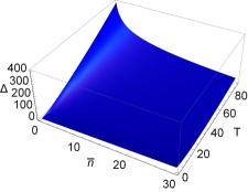
(a)  (b)

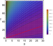
Figure 3: (a) $\Delta$ parameter as a function of $T$ and $\bar{n}$ for the thermal light state and the Hamiltonian of a degenerated parametric amplifier. (b) Contour plots of the $\Delta$ parameter, the red line corresponds to $T=\bar{n}$. The Hamiltonian parameters used are: $\omega_{0}=\omega_{t}=1$, $\omega=3$ and $k=0.1$.

5 Summary and concluding remarks

In this work, we analyzed the Tsallis relative entropy between the states $\hat{\rho}$ and $\hat{\sigma}$: $S_{q}(\hat{\rho},\hat{\sigma})$ for $q=1+\delta$ ($\delta\ll 1$, $\delta>0$). The result is expressed in terms of powers of $\delta$. Studying the first term of the series (the von Neumann relative entropy), we defined a parameter $\Delta$ that measures the distance between an arbitrary density $\hat{\rho}$ and a thermal equilibrium state $\hat{\sigma}=e^{-\beta\hat{H}}/{\rm Tr}(e^{-\beta\hat{H}})$. This parameter can be expressed in terms of the energy $E(\hat{\rho},\hat{H})$, the entropy $S(\hat{\rho})$ and the partition function $Z(\beta,\hat{H})$ of the system. We studied this parameter for a general qubit system and unimodal Gaussian state.

Also we showed that a qubit system is equal to a thermal equilibrium state, if the Bloch vectors of the state $\mathbf{p}$ and the Hamiltonian $\mathbf{h}$ follow the relation $\mathbf{p}=-\mathbf{h}\tanh(\beta|\mathbf{h}|/2)/|\mathbf{h}|$. This condition implies that the two Bloch vectors are antiparallel for $T\geq 0$ and parallel for $T<0$. In both cases, the temperature where $\Delta=0$ is given by $T=|\mathbf{h}|/(2\,{\rm arctanh}|\mathbf{p}|)$.

In the Gaussian case, the general partition function for a quadratic Hamiltonian was obtained in order to calculate $\Delta$. As an example, we presented the comparison between the thermal light state and a thermal equilibrium state given by the parametric amplifier Hamiltonian. We demonstrated that, in the case of small interaction constant $k$ of the parametric amplifier, there is a region ($T\approx\bar{n}$) where $\Delta$ is minimum.

Appendix A Partition function for unimodal quadratic Hamiltonian systems

The partition function associated to the arbitrary unimodal quadratic Hamiltonian of Eq. (12) is obtained in this section. It is possible to see that the quadratic Hamiltonian $\hat{H}$ can be expressed in terms of the SU(1,1) operators $\hat{K}_{+}=\hat{a}^{\dagger 2}/2$, $\hat{K_{-}}=\hat{a}^{2}/2$ and $\hat{K}_{0}=(\hat{a}^{\dagger}\hat{a}+1/2)/2$ as follows

$$\hat{H}=2\left(\gamma_{1}\hat{K}_{-}+\gamma_{1}^{*}\hat{K}_{+}+\left(\frac{\omega_{3}}{\omega_{0}}+\omega_{0}\omega_{1}\right)\hat{K}_{0}\right)+\textrm{Im}(\omega_{2}),$$

where $\gamma_{1}=(\omega_{3}/\omega_{0}-\omega_{0}\omega_{1}-2i\,{\rm Re}(\omega_{2}))/2$. Because of this property the exponential operator $e^{-\beta\hat{H}}$ can be decompose as the product of exponential of each element of the algebra i.e.,

$$e^{-\beta\hat{H}}=e^{-\beta\,\textrm{Im}(\omega_{2})}e^{A_{+}\hat{K}_{+}}e^{\ln(A_{0})\hat{K}_{0}}e^{A_{-}\hat{K}_{-}}$$

where

$$A_{+}=\frac{(-2\beta\gamma_{1}^{*}/\phi)\sinh\phi}{\cosh\phi+(\beta(\omega_{0}\omega_{1}+\frac{\omega_{3}}{\omega_{0}})/\phi)\sinh\phi},\quad A_{-}=\frac{(-2\beta\gamma_{1}/\phi)\sinh\phi}{\cosh\phi+(\beta(\omega_{0}\omega_{1}+\frac{\omega_{3}}{\omega_{0}})/\phi)\sinh\phi},$$

$$A_{0}=\left(\cosh\phi+\frac{\beta(\omega_{0}\omega_{1}+\frac{\omega_{3}}{\omega_{0}})}{\phi}\sinh\phi\right)^{-2},\quad\phi=\beta\left(\left(\omega_{0}\omega_{1}+\frac{\omega_{3}}{\omega_{0}}\right)^{2}-4|\gamma_{1}|^{2}\right)^{1/2}.$$

The diagonal matrix elements in the Fock representation of the exponential operator can be expressed in terms of the Legendre polynomials $P_{n}(z)$

$$\langle n|e^{-\beta\hat{H}}|n\rangle=e^{-\beta\,\textrm{Im}(\omega_{2})}A_{0}^{1/4}(A_{0}(1-\xi))^{n/2}P_{n}\left(\frac{1}{\sqrt{1-\xi}}\right),\quad\xi=\frac{A_{+}A_{-}}{A_{0}},$$

summing this elements over $n$ we finally have

$$Z(\beta,\hat{H})=\frac{A_{0}^{1/4}e^{-\beta\,\textrm{Im}(\omega_{2})}}{\sqrt{1-2A_{0}^{1/2}+A_{0}(1-\xi)}},$$

renaming $A_{0}=\zeta$ we arrive to the expression for the partition function of Eq. (14).

References

References

- [1] J. Goold, M. Huber, A. Riera, L. del Rio, P. Skrzypczyk, The role of quantum information in thermodynamics a topical review, J. of Phys. A 49 (14) (2016) 143001.
- [2] J. M. R. Parrondo, J. M. Horowitz, T. Sagawa, Thermodynamics of information, Nat. Phys. 11 (2) (2015) 131–139.
- [3] L. Szilard, Über die entropieverminderung in einem thermodynamischen system bei eingriffen intelligenter wesen, Z. Physik 53 (11) (1929) 840–856.
- [4] K. Maruyama, F. Nori, V. Vedral, The physics of maxwell’s demon and information, Rev. Mod. Phys. 81 (2009) 1–23.
- [5] L. Amico, R. Fazio, A. Osterloh, V. Vedral, Entanglement in many-body systems, Rev. Mod. Phys. 80 (2008) 517–576.
- [6] M. Esposito, C. V. den Broeck, Second law and landauer principle far from equilibrium, Europhys. Lett. 95 (4) (2011) 40004.
- [7] F. G. S. L. Brandão, M. Horodecki, J. Oppenheim, J. M. Renes, R. W. Spekkens, Resource theory of quantum states out of thermal equilibrium, Phys. Rev. Lett. 111 (2013) 250404.
- [8] P. Skrzypczyk, A. J. Short, S. Popescu, Work extraction and thermodynamics for individual quantum systems, Nat. Comm. 5 (2014) 4185.
- [9] P. Faist, F. Dupuis, J. Oppenheim, R. Renner, The minimal work cost of information processing, Nat. Comm. 6 (2015) 7669.
- [10] N. Yunger Halpern, P. Faist, J. Oppenheim, A. Winter, Microcanonical and resource-theoretic derivations of the thermal state of a quantum system with noncommuting charges, Nat. Comm. 7 (2016) 12051.
- [11] J. von Neumann, Mathematical foundations of quantum mechanics, Princeton University Press, Princeton N.J, 1955.
- [12] C. Tsallis, Possible generalization of boltzmann-gibbs statistics, J. of Stat. Phys. 52 (1) (1988) 479–487.
- [13] M. A. Man’ko, V. I. Man’ko, G. Marmo, Entropies and correlations in classical and quantum systems, Il Nuovo Cimento C 38 (2016) 167.
- [14] E. O. Kiktenko, A. K. Fedorov, O. V. Man’ko, V. I. Man’ko, Multilevel superconducting circuits as two-qubit systems: Operations, state preparation, and entropic inequalities, Phys. Rev. A 91 (2015) 042312.
- [15] E. Kiktenko, A. Fedorov, A. Strakhov, V. Man’ko, Single qudit realization of the deutsch algorithm using superconducting many-level quantum circuits, Phys. Lett. A 379 (22) (2015) 1409 – 1413.
- [16] E. Glushkov, A. Glushkova, V. I. Man’ko, Testing entropic inequalities for superconducting qudits, J. of Russ. Laser Res. 36 (5) (2015) 448–457.
- [17] M. A. Nielsen, I. L. Chuang, Quantum Computation and Quantum Information: 10th Anniversary Edition, 10th Edition, Cambridge University Press, New York, NY, USA, 2011.
- [18] B. Gaveau, L. Schulman, A general framework for non-equilibrium phenomena: the master equation and its formal consequences, Phys. Lett. A 229 (6) (1997) 347 – 353.
- [19] A. Figueroa, J. López, O. Castaños, R. López-Peña, M. A. Man’ko, V. I. Man’ko, Entropy energy inequalities for qudit states, J. of Phys. A 48 (6) (2015) 065301.
- [20] H. Hasegawa, divergence of the non-commutative information geometry, Rep. on Math. Phys. 33 (1) (1993) 87 – 93.
- [21] C. Weedbrook, S. Pirandola, R. García-Patrón, N. J. Cerf, T. C. Ralph, J. H. Shapiro, S. Lloyd, Gaussian quantum information, Rev. Mod. Phys. 84 (2012) 621–669.
- [22] G. Adesso, S. Ragy, A. R. Lee, Continuous variable quantum information: Gaussian states and beyond, Open Sys. and Inf. Dyn. 21 (01n02) (2014) 1440001.
- [23] M. Ban, Decomposition formulas for su(1, 1) and su(2) lie algebras and their applications in quantum optics, J. Opt. Soc. Am. B 10 (8) (1993) 1347–1359.
- [24] A. Serafini, F. Illuminati, S. D. Siena, Symplectic invariants, entropic measures and correlations of gaussian states, J. of Phys. B 37 (2) (2004) L21.
- [25] W. H. Louisell, A. Yariv, A. E. Siegman, Quantum fluctuations and noise in parametric processes. i., Phys. Rev. 124 (1961) 1646–1654.