3D Deformable Object Manipulation using Fast Online Gaussian Process Regression

Abstract

In this paper, we present a general approach to automatically visual-servo control the position and shape of a deformable object whose deformation parameters are unknown. The servo-control is achieved by online learning a model mapping between the robotic end-effector’s movement and the object’s deformation measurement. The model is learned using the Gaussian Process Regression (GPR) to deal with its highly nonlinear property, and once learned, the model is used for predicting the required control at each time step. To overcome GPR’s high computational cost while dealing with long manipulation sequences, we implement a fast online GPR by selectively removing uninformative observation data from the regression process. We validate the performance of our controller on a set of deformable object manipulation tasks and demonstrate that our method can achieve effective and accurate servo-control for general deformable objects with a wide variety of goal settings. Experiment videos are available at https://sites.google.com/view/mso-fogpr.

I Introduction

Manipulation of deformable objects is a challenging problem in robotic manipulation and has many important applications, including cloth folding [1, 2], string insertion [3], sheet tension [4], robot-assisted surgery [5], and suturing [6].

Most previous work on robotic manipulation can be classified into two categories: some approaches did not explicitly model the deformation parameters of the object, and used vision or learning methods to accomplish tasks [1, 7, 6, 8, 9, 10, 11, 12]. These methods focus on high-level policies but lack the capability to achieve accurate operation – actually most of them are open-loop methods. Other approaches require a model about the object’s deformation properties in terms of stiffness, Young’ modules, or FEM coefficients, to design a control policy [13, 5, 14, 15, 16, 17]. However, such deformation parameters are difficult to be estimated accurately and may even change during the manipulation process, especially for objects made by nonlinear elastic or plastic materials. These challenges leave the automatic manipulation of deformable objects an open research problem in robotics [18].

In this paper, we focus on designing servo-manipulation algorithm which can learn a nonlinear deformation function along with the manipulation process. The deformation function is efficiently learned using a novel online Gaussian process regression and is able to model the relation between the movement of the robotic end-effectors and the soft object’s deformation adaptively during the manipulation. In this way, we design a nonlinear feedback controller that makes a good balance between exploitation and exploration and provides better convergence and dynamic behavior than previous work using linear deformation models such as  [15, 16]. Our manipulation system successfully and efficiently accomplishes a set of different manipulation tasks for a wide variety of objects with different deformation properties.

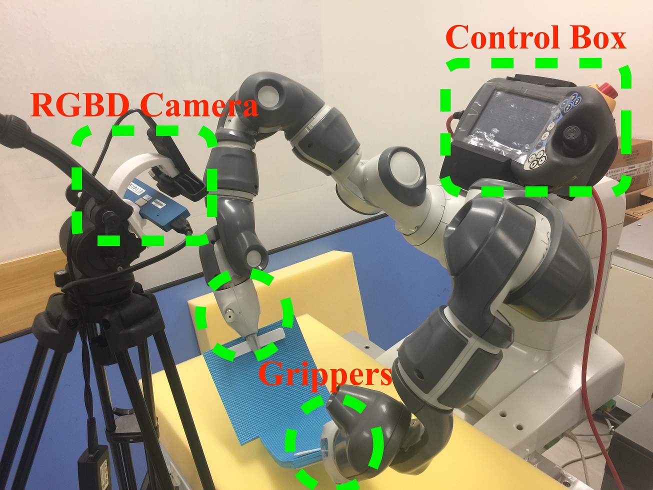
Figure 1: Our robotic system for deformable object manipulation is made by two 3D cameras and one dual-arm ABB robot.

II Related Work

Many robotic manipulation method for deformable objects have been proposed recent years. Early work [19, 20] used knot theory or energy theory to plan the manipulation trajectories for linear deformable objects like ropes. Some recent work [21] further considered manipulating cloths using dexterous cloths. These work required a complete and accurate knowledge about the object’ geometric and deformation parameters and thus are not applicable in practice.

More practical work used sensors to guide the manipulation process.  [22] used image to estimate the knot configuration.  [1] used vision to estimate the configuration of a cloth and then leverage gravity to accomplish folding tasks [23].  [7] used RGBD camera to identify the boundary components in clothes.  [11, 12] first used vision to determine the status of the cloth, then optimized a set of grasp points to unfold the clothes on the table, and finally found a sequence of folding actions. Schulman et al. [6] enabled a robot to accomplish complex multi-step deformation object manipulation strategies by learning from a set of manipulation sequences with depth images to encode the task status. Such learning from demonstration technique has further been extended using reinforcement learning [8] and tangent space mapping [9]. A deep learning-based end-to-end framework has also been proposed recently [10]. A complete pipeline for clothes folding task including vision-based garments grasping, clothes classification and unfolding, model matching and folding has been described in [24].

Above methods generally did not explicitly model the deformation parameters of the deformation objects, which is necessary for high-quality manipulation control. Some methods used uncertainty model [13] or heuristics [25, 3] to take into account rough deformation models during the manipulation process. Some work required an offline procedure to estimate the deformation parameters [14]. There are several recent work estimating the object’s deformation parameters in an online manner and then design controller accordingly. Navarro-Alarcon et al. [15, 16] used an adaptive and model-free linear controller to servo-control soft objects, where the object’s deformation is modeled using a spring model [26]. [17] learned the models of the part deformation depending on the end-effector force and grasping parameters in an online manner to accomplish high-quality cleaning task. A more complete survey about deformable object manipulation in industry is available in[18].

In this paper, we are using Gaussian process regression (GPR) to model and learn the deformation parameters of a soft object. Our method is motivated by several recent work focus on reducing the computational cost of the offline GPR.  [27] presented a sparse GPR method by selecting $M$ pseudo-input points from the $N$ training data to balance the computational cost and the model accuracy, where $M\ll N$.  [28, 29] divided the input space of the Gaussian process model into smaller subspaces, and fit a local GPR for each subspace.  [30] used many local GPRs and updated local models iteratively, in order to reduce the training time. Our method proposed an online sparse method for efficient deformation model adaptation during the manipulation process.

III Overview and Problem Formulation

The problem of 3D deformable object manipulation can be formulated as follows. Similar to [26], we describe an object as a set of discrete points, which are classified into three types: the manipulated points, the feedback points, and the uninformative points, as shown in Figure 2. The manipulated points correspond to the positions on the object that are grabbed by the robot and thus is fixed relative to the robotic end-effectors; the feedback points correspond to the object surface regions that define the task goal setting and involve in the visual feedbacks; and the uninformative points correspond to other regions on the object. Given this setup, the deformable object manipulation problem is about how to move the manipulated points in order to drive the feedback points toward a required target configuration.

Since the manipulation of deformable object is usually executed at a low speed to avoid vibration, we can reasonably assume that the object always lies in the quasi-static state where the internal forces caused by the elasticity of the object is balanced with the external force applied by the end-effector on the manipulated points. We use a potential energy function $U(\mathbf{p}^{m},\mathbf{p}^{f},\mathbf{p}^{u})$ to formulate the elasticity of the deformable object, where the potential energy depends on all the points on the object, and vectors $\mathbf{p}^{m}$, $\mathbf{p}^{f}$ and $\mathbf{p}^{u}$ represent the stacked coordinates of all manipulated points, feedback points and uninformed points, respectively. The equation of equilibrium for the object can then be described as follows:

$$\frac{\partial U}{\partial\mathbf{p}^{m}}-\mathbf{F} =\mathbf{0},$$ (1)

$$\frac{\partial U}{\partial\mathbf{p}^{f}} =\mathbf{0},$$ (2)

$$\frac{\partial U}{\partial\mathbf{p}^{u}} =\mathbf{0},$$ (3)

where $\mathbf{F}$ is the external force vector applied on the manipulated points. To solve the above equations, we need exact knowledge about that deformable object’s deformation property, which is not available or difficult to acquire in many applications. To cope with this issue, we first simplify the potential energy function to only depend on $\mathbf{p}^{m}$ and $\mathbf{p}^{f}$, which is reasonable because usually the uninformed points are far from the manipulated and feedback points and thus their influence on the manipulation process is small and can be neglected. Next, we perform Taylor expansion of Equation 1 and Equation 2 about the current static equilibrium status $(\mathbf{p}^{f}_{*},\mathbf{p}^{m}_{*})$, and the equation of equilibrium implies a relationship between the relative displacements of feedback points and the manipulated points:

$$A(\delta\mathbf{p}^{f})+B(\delta\mathbf{p}^{m})=\mathbf{0},$$ (4)

where $\delta\mathbf{p}^{f}=\mathbf{p}^{f}-\mathbf{p}^{f}_{*}$ and $\delta\mathbf{p}^{m}=\mathbf{p}^{m}-\mathbf{p}^{m}_{*}$ are the displacement relative to the equilibrium for feedback points and manipulated points, respectively. The functions $A(\cdot)$ and $B(\cdot)$ are nonlinear in general, though they can be linear in some special cases. For instance, when only performing the first order Taylor expansion as what is done in [16], $A(\delta\mathbf{p}^{f})=\frac{\partial^{2}U}{\partial\mathbf{p}^{m}\partial\mathbf{p}^{f}}$ and $B(\delta\mathbf{p}^{m})=\frac{\partial^{2}U}{\partial(\mathbf{p}^{m})^{2}}\delta\mathbf{p}^{m}$ are two linear functions. In this paper, we allow $A(\cdot)$ and $B(\cdot)$ to be general smooth linear functions to estimate a better model for the deformable object manipulation process.

We further assume the function $B(\cdot)$ to be invertible, which implies

$$\delta\mathbf{p}^{m}=D(\delta\mathbf{p}^{f}),$$ (5)

where $D=A\circ B^{-1}$ is the mapping between the velocities of the feedback points and the manipulated points. In this way, we can determine a suitable end-effector velocity via feedback control $\delta_{p}^{m}=D(\eta\cdot\Delta\mathbf{p}^{f})$ to derive the object toward its goal state, where $\Delta\mathbf{p}^{f}=\mathbf{p}^{f}_{d}-\mathbf{p}^{f}$ is the difference between the desired vector and the current vector of the feedback points and $\eta$ is the feedback gain.

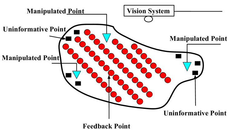
Figure 2: We model a soft object using three classes of points： manipulated points, feedback points, and uninformative points.

However, the velocities of feedback points usually cannot be directly used in the control, because in practice these velocities are measured using visual tracking of deformable objects and thus are likely to be noisy or even unreliable when tracking fails. More importantly, a soft object needs a large set of feedback points to characterize its deformation, but a robotic manipulation system usually only has a few end-effectors, and thus the $D(\cdot)$ function is Equation 5 is a mapping from the high-dimensional space of feedback point velocities to the low-dimensional space of manipulated point velocities. Such a system is extremely underactuated and thus the convergence speed of the control would be slow.

To deal with aforementioned difficulties, we extract a low-dimensional feature vector $\mathbf{x}$ from the feedback points for the control purpose, where $\mathbf{x}=C(\mathbf{p}^{f})$ is a feature vector whose dimension is much smaller than that of $\mathbf{p}^{f}$, and the function $C(\cdot)$ is the feature extraction function. Around the equilibrium state, we have $\delta\mathbf{x}=C^{\prime}(\mathbf{p}^{f}_{*})\delta\mathbf{p}^{f}_{*}$, and can rewrite the equilibrium function using the feature vector as

$$\delta\mathbf{p}^{m}=D(C^{\prime}(\mathbf{p}^{f}_{*})^{-1}\delta\mathbf{x})\triangleq H(\delta\mathbf{x}),$$ (6)

where the function $H(\cdot)$ is called the deformation function.

The manipulation problem of deformable object can finally be described as: given the desired state $\mathbf{x}_{d}$ of an object in the feature space, design a controller which learns the nonlinear function $H(\cdot)$ in an online manner, and outputs the control velocity $\delta\mathbf{p}^{m}$ decreasing the distance between the object’s current state $\mathbf{x}$ and $\mathbf{x}_{d}$, i.e. $\delta\mathbf{p}^{m}=H(\eta\cdot\Delta\mathbf{x})$, where $\Delta\mathbf{x}=\mathbf{x}_{d}-\mathbf{x}$ and $\eta$ is the feedback gain.

IV Controller Design

IV-A Deformation Function Learning

Since the deformation function $H(\cdot)$ is a general and highly nonlinear function determining how the movement of the manipulated points is converted into the feature space, the learning of the function $H$ requires a flexible and non-parametric method. Our solution is to use the Gaussian Process Regression (GPR) to fit the deformation function in an online manner.

GPR is a nonparametric regression technique which defines a distribution over functions and the inference takes place directly in the functional space given the covariance and mean of the functional distribution. For our manipulation problem, we formulate the deformation function $H$ as a Gaussian process:

$$H\sim GP\left(m(\delta\mathbf{x}),\,\,k(\delta\mathbf{x},\delta\mathbf{x}^{\prime})\right)$$ (7)

where $\delta\mathbf{x}$ still denotes the velocity in the feature space. For the covariance or kernel function $k(\delta\mathbf{x},\delta\mathbf{x}^{\prime})$, we are using the Radius Basis Function (RBF) kernel: $k(\delta\mathbf{x},\delta\mathbf{x}^{\prime})=\exp(-\frac{\|\delta\mathbf{x}-\delta\mathbf{x}^{\prime}\|^{2}}{2\sigma_{RBF}^{2}})$, where the parameter $\sigma_{RBF}$ sets the spread of the kernel. For the mean function $m(\delta\mathbf{x})$, we are using the linear mean function $m(\delta\mathbf{x})=\mathbf{W}\delta\mathbf{x}$, $\mathbf{W}$ is the linear regression weight matrix. We choose to use a linear mean function rather than the common zero mean function, because previous work [16] showed that a linear function can capture a large part of the deformation function $H$. As a result, a linear mean function can result in faster convergence of our online learning process and also provide a relatively accurate prediction in the unexplored region in the feature space. The matrix $W$ is learned online by minimizing a squared error $Q=\frac{1}{2}\|\delta\mathbf{p}^{m}-\mathbf{W}\delta\mathbf{x}\|_{2}$ with respect to the weight matrix $\mathbf{W}$.

Given a set of training data in terms of pairs of feature space velocities and manipulated point velocities $\{(\delta\mathbf{x}_{t},\delta\mathbf{p}^{m}_{t})\}_{t=1}^{N}$ during the previous manipulation process, the standard GPR computes the distribution of the deformation function as a Gaussian process $H(\delta\mathbf{x})\sim\mathcal{N}(\mu(\delta\mathbf{x}),\sigma^{2}(\delta\mathbf{x}))$, where GP’s mean function is

$$\mu(\delta\mathbf{x}) =m(\delta\mathbf{x})+\mathbf{k}^{T}(\delta\mathbf{X},\delta\mathbf{x})\cdot[\mathbf{K}(\delta\mathbf{X},\delta\mathbf{X})+\sigma_{n}^{2}\mathbf{I}]^{-1}$$

$$\quad\cdot(\delta\mathbf{P}^{m}-m(\delta\mathbf{X}))$$ (8)

and GP’s covariance function is

$$\sigma^{2}(\delta\mathbf{x}) =k(\delta\mathbf{x},\delta\mathbf{x})-\mathbf{k}^{T}(\delta\mathbf{X},\delta\mathbf{x})\cdot[\mathbf{K}(\delta\mathbf{X},\delta\mathbf{X})+\sigma_{n}^{2}\mathbf{I}]^{-1}$$

$$\quad\cdot\mathbf{k}(\delta\mathbf{X},\delta\mathbf{x}).$$ (9)

Here $\delta\mathbf{X}$ and $\delta\mathbf{P}^{m}$ are matrices corresponding to the stack of $\{\delta\mathbf{x}_{t}\}_{t=1}^{N}$ and $\{\delta\mathbf{p}^{m}_{t}\}_{t=1}^{N}$ in the training data, respectively. $\mathbf{K}$ and $\mathbf{k}$ are matrices and vectors computed using a given covariance function $k(\cdot,\cdot)$. The matrix $\mathbf{A}=\mathbf{K}+\sigma_{n}^{2}\mathbf{I}$ is called the Gram matrix, and the parameter $\sigma_{n}$ estimates the uncertainty or noise level of the training data.

IV-B Real-time Online GPR

In the deformation object manipulation process, the data $(\delta\mathbf{x}_{t},\delta\mathbf{p}_{t}^{m})$ is generated sequentially, and thus at each time step $t$, we need to update the GP deformation function $H_{t}(\delta\mathbf{x})\sim\mathcal{N}(\mu_{t}(\delta\mathbf{x}),\sigma^{2}(\delta\mathbf{x}))$ at an interactive manner, with

$$\mu_{t}(\delta\mathbf{x}) =m(\delta\mathbf{x})+\mathbf{k}^{T}(\delta\mathbf{X}_{t},\delta\mathbf{x})\cdot[\mathbf{K}(\delta\mathbf{X}_{t},\delta\mathbf{X}_{t})+\sigma_{n}^{2}\mathbf{I}]^{-1}$$

$$\quad\cdot(\delta\mathbf{P}^{m}_{t}-m(\delta\mathbf{X}_{t}))$$ (10)

and

$$\sigma^{2}_{t}(\delta\mathbf{x}) =k(\delta\mathbf{x},\delta\mathbf{x})-\mathbf{k}^{T}(\delta\mathbf{X}_{t},\delta\mathbf{x})\cdot[\mathbf{K}(\delta\mathbf{X}_{t},\delta\mathbf{X}_{t})+\sigma_{n}^{2}\mathbf{I}]^{-1}$$

$$\quad\cdot\mathbf{k}(\delta\mathbf{X}_{t},\delta\mathbf{x}).$$ (11)

In the online GPR, we need to perform the inversion of the Gram matrix $\mathbf{A}_{t}=\mathbf{K}(\delta\mathbf{X}_{t},\delta\mathbf{X}_{t})+\sigma_{n}^{2}\mathbf{I}$ repeatedly with a time complexity $\mathcal{O}(N^{3})$, where $N$ is the size of the current training set involved in the regression. Such cubic complexity makes the training process slow for long manipulation sequence where the training data size $N$ increases quickly. In addition, the growing up of the GP model will reduce the newest data’s impact on the regression result and make the GP fail to capture the change of the objects’s deformation parameters during the manipulation. This is critical for deformable object manipulation, because the deformation function $H$ is derived from the local force equilibrium and thus is only accurate in a small region.

Motivated by previous work about efficient offline GPR [27, 28, 29, 30], we here present a novel online GPR method called the Fast Online GPR (FO-GPR) to reduce the high computational cost and to adapt to the changing deformation properties while updating the deformation model during the manipulation process. The main idea of FO-GPR includes two parts: 1) maintaining the inversion of the Gram matrix $\mathcal{A}_{t}$ incrementally rather using direct matrix inversion; 2) restricting the size of $\mathbf{A}_{t}$ to be smaller than a given size $M$, and $\mathbf{A}_{t}$’s size exceeds that limit, using a selective “forgetting” method to replace stale or uninformative data by the fresh new data point.

IV-B1 Incremental Update of Gram matrix $\mathbf{A}_{t}$

Suppose at time $t$, the size of $\mathbf{A}_{t}$ is still smaller than the limit $M$. In this case, $A_{t}$ and $A_{t-1}$ are related by

$$\mathbf{A}_{t}=\begin{bmatrix}\mathbf{A}_{t-1}&\mathbf{b}\\ \mathbf{b}^{T}&c\end{bmatrix},$$ (12)

where $\mathbf{b}=\mathbf{k}(\delta\mathbf{X}_{t-1},\delta\mathbf{x}_{t})$ and $c=k(\delta\mathbf{x}_{t},\delta\mathbf{x}_{t})+\sigma^{2}_{n}$. According to the Helmert-–Wolf blocking inverse property, we can compute the inverse of $\mathbf{A}_{t}$ based on the inverse of $\mathbf{A}_{t-1}$:

$$\mathbf{A}_{t}^{-1} =\begin{bmatrix}\left(\mathbf{A}_{t-1}-\frac{1}{c}\mathbf{bb}^{T}\right)^{-1}&-\frac{1}{r}\mathbf{A}_{t-1}^{-1}\mathbf{b}\\ -\frac{1}{r}\mathbf{b}^{T}\mathbf{A}_{t-1}^{-1}&\frac{1}{r}\end{bmatrix}$$

$$=\begin{bmatrix}\mathbf{A}_{t-1}^{-1}+\frac{1}{r}\mathbf{A}_{t-1}^{-1}\mathbf{bb}^{T}\mathbf{A}_{t-1}^{-1}&-\frac{1}{r}\mathbf{A}_{t-1}^{-1}\mathbf{b}\\ -\frac{1}{r}\mathbf{A}_{t-1}^{T}\mathbf{A}_{t-1}^{-1}&\frac{1}{r}\end{bmatrix},$$ (13)

where $r=c-\mathbf{b}^{T}\mathbf{A}_{t-1}^{-1}\mathbf{b}$. In this way, we achieve the incremental update of the inverse Gram matrix from $\mathbf{A}_{t-1}^{-1}$ to $\mathbf{A}_{t}^{-1}$, and the computational cost is $\mathcal{O}(N^{2})$ rather than $\mathcal{O}(N^{3})$ of direct matrix inversion. This acceleration enables fast GP model update during the manipulation process.

IV-B2 Selective Forgetting in Online GPR

When the size of $\mathbf{A}_{t-1}$ reaches the limit $M$, we use a “forgetting” strategy to replace the most uninformative data by the fresh data points while keeping the size of $\mathbf{A}_{t}$ to be $M$. In particular, we choose to forget the $i_{*}$ data point that is the most similar to other data points in terms of the covariance, i.e.,

$$i_{*}=\operatorname*{\arg\!\max}_{i}\sum\nolimits_{j}\mathbf{A}[i,j],$$ (14)

where $\mathbf{A}[i,j]$ denotes the covariance value stored in the $i$-th row and $j$-th column in $\mathbf{A}$, i.e., $k(\delta\mathbf{x}_{i},\delta\mathbf{x}_{j})+\sigma_{n}^{2}$.

Given the new data $(\delta\mathbf{x}_{t},\delta\mathbf{p}^{m}_{t})$, we need to update $\delta\mathbf{X}_{t}$, $\delta\mathbf{P}^{m}_{t}$, and $\mathbf{A}_{t}^{-1}=[\mathbf{K}(\delta\mathbf{X}_{t},\delta\mathbf{X}_{t})+\sigma_{n}^{2}\mathbf{I}]^{-1}$ in Equation IV-B and IV-B by swapping data terms related to $\delta\mathbf{x}_{t}$ and $\delta\mathbf{x}_{i_{*}}$, in order to update the deformation function $H_{t}$.

The incremental update for $\delta\mathbf{X}_{t}$ and $\delta\mathbf{P}_{m}^{t}$ is trivial: $\delta\mathbf{X}_{t}$ is identical to $\delta\mathbf{X}_{t-1}$ except $\delta\mathbf{X}_{t}[i_{*}]$ is $\delta\mathbf{x}_{t}$ rather than $\delta\mathbf{x}_{i_{*}}$; $\delta\mathbf{P}_{t}^{m}$ is identical to $\delta\mathbf{P}_{t-1}^{m}$ except $\delta\mathbf{P}_{t}^{m}[i_{*}]$ is $\delta\mathbf{p}_{t}^{m}$ rather than $\delta\mathbf{p}_{i_{*}}^{m}$.

We then discuss how to update $\mathbf{A}_{t}$ from $\mathbf{A}_{t-1}$. Since $\mathbf{A}_{t}-\mathbf{A}_{t-1}$ is only non-zero at the $i_{*}$-th column or the $i_{*}$-th row:

$$(\mathbf{A}_{t}-\mathbf{A}_{t-1})[i,j]=\begin{cases}0,&i,j\neq i_{*}\\ k(\delta\mathbf{x}_{i},\delta\mathbf{x})-k(\delta\mathbf{x}_{i},\delta\mathbf{x}_{i_{*}}),&j=i_{*}\\ k(\delta\mathbf{x}_{j},\delta\mathbf{x})-k(\delta\mathbf{x}_{j},\delta\mathbf{x}_{i_{*}}),&i=i_{*},\end{cases}$$

this matrix can be written as the multiplication of two matrices $\mathbf{U}$ and $\mathbf{V}$, i.e. $\mathbf{A}_{t}-\mathbf{A}_{t-1}=\mathbf{U}\mathbf{V}^{T}$, where

$$\mathbf{U}=\begin{bmatrix}\mathbf{e}_{i_{*}}&(\mathbf{I}-\frac{1}{2}\mathbf{e}_{i_{*}}\mathbf{e}_{i_{*}}^{T})(\mathbf{k}_{t}-\mathbf{k}_{t-1})\end{bmatrix}$$

and

$$\mathbf{V}=\begin{bmatrix}(\mathbf{I}-\frac{1}{2}\mathbf{e}_{i_{*}}\mathbf{e}_{i_{*}}^{T})(\mathbf{k}_{t}-\mathbf{k}_{t-1})&\mathbf{e}_{i_{*}}\end{bmatrix}.$$

Here $\mathbf{e}_{i_{*}}$ is a vector that is all zero but one at the $i_{*}$-th item, $\mathbf{k}_{t}$ is the vector $\mathbf{k}(\delta\mathbf{X}_{t},\delta\mathbf{x}_{t})$ and $\mathbf{k}_{t-1}$ is the vector $\mathbf{k}(\delta\mathbf{X}_{t-1},\delta\mathbf{x}_{i_{*}})$. Both $\mathbf{U}$ and $\mathbf{V}$ are size $M\times 2$ matrices.

Then using Sherman-Morrison formula, there is

$$\mathbf{A}_{t}^{-1} =(\mathbf{A}_{t-1}+\mathbf{U}\mathbf{V}^{T})^{-1}$$ (15)

$$=\mathbf{A}_{t-1}^{-1}-\mathbf{A}_{t-1}^{-1}\mathbf{U}(\mathbf{I}+\mathbf{V}^{T}\mathbf{A}_{t-1}^{-1}\mathbf{U})^{-1}\mathbf{V}^{T}\mathbf{A}_{t-1}^{-1},$$

which provides the incremental update scheme for the Gram matrix $\mathbf{A}_{t}$. Since $\mathbf{I+V}^{T}\mathbf{A}_{t-1}^{-1}\mathbf{U}$ is a $2\times 2$ matrix, its inversion can be computed in $\mathcal{O}(1)$ time. Therefore, the incremental update computation is dominated by the matrix-vector multiplication and thus the time complexity is $\mathcal{O}(M^{2})$ rather than $\mathcal{O}(M^{3})$.

A complete description for FO-GPR is as shown in Algorithm 1.

Algorithm 1 FO-GPR

0:  $\delta\mathbf{X}_{t-1}$, $\delta\mathbf{P}^{m}_{t-1}$, $\mathbf{A}_{t-1}$, $\delta\mathbf{x}_{t}$, $\delta\mathbf{p}^{m}_{t}$

0:  $\delta\mathbf{X}_{t}$, $\delta\mathbf{P}^{m}_{t}$, $\mathbf{A}_{t}^{-1}$

1:  if $dim(\mathbf{A}_{t-1})<M$ then

2:     $\delta\mathbf{X}_{t}=[\delta\mathbf{X}_{t-1},\delta\mathbf{x}_{t}]$

3:     $\delta\mathbf{P}^{m}_{t}=[\delta\mathbf{P}^{m}_{t-1},\delta\mathbf{p}_{t}^{m}]$

4:     $\mathbf{A}_{t}^{-1}$ computed using Equation IV-B1

5:  else

6:     $i_{*}$ computed using Equation 14

7:     $\delta\mathbf{X}_{t}=\delta\mathbf{X}_{t-1}$, $\delta\mathbf{X}_{t}[i_{*}]=\delta\mathbf{x}_{t}$

8:     $\delta\mathbf{P}_{t}^{m}=\delta\mathbf{P}_{t-1}^{m}$, $\delta\mathbf{P}_{t}^{m}[i_{*}]=\delta\mathbf{p}^{m}_{t}$

9:     $\mathbf{A}_{t}^{-1}$ computed using Equation 15

10:  end if

IV-C Exploitation and Exploration

Given the deformation function $H_{t}$ learned by FO-GPR, the controller system predicts the required velocity to be executed by the end-effectors based on the error between the current state and the goal state in the feature space:

$$\delta\mathbf{p}^{m}=H_{t}(\eta\cdot(\mathbf{x}^{d}-\mathbf{x})),$$ (16)

where $\eta$ is a scale factor as the feedback gain.

However, when there is no sufficient data, GPR cannot output control policy with high confidence, which typically happens in the early step of the manipulation or when the robot manipulates the object into a new unexplored configuration. Fortunately, the GPR framework provides a natural way to trade-off exploitation and exploration by sampling the control velocity from distribution of $H_{t}$:

$$\delta\mathbf{p}^{m}\sim\mathcal{N}(\mu_{t},\sigma_{t}^{2})$$ (17)

If $\mathbf{x}_{t}$ is now in unexplored region with large $\sigma_{t}^{2}$, the controller will perform exploration around $\mu_{t}$; if $\mathbf{x}_{t}$ is in a well-explored region with small $\sigma_{t}^{2}$, the controller will output velocity close to $\mu_{t}$.

A complete description of the controller based on FO-GPR is shown in Figure 3.

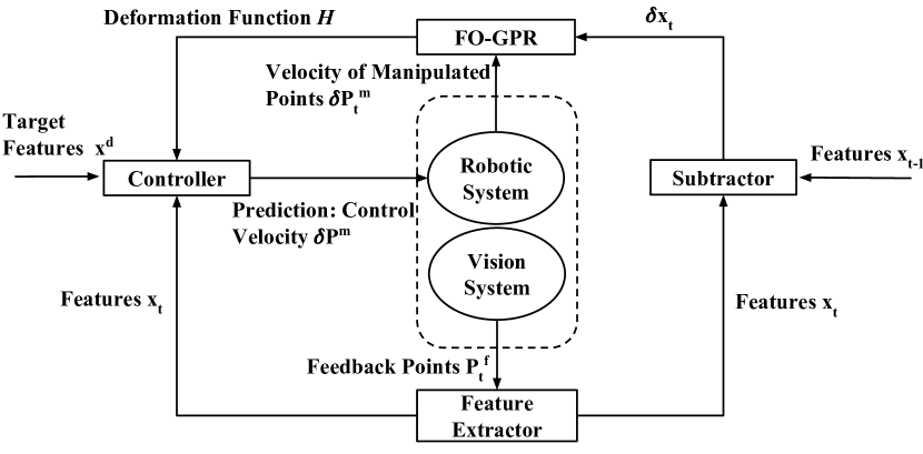
Figure 3: An overview of our deformable object manipulation system.

V Feature Extraction

For rigid body manipulation, an object’s state can be completely described by its centroid position and orientation. But such global features are not sufficient to determine the configuration of a deformable object. As mentioned in Section IV, we extract a feature vector $\mathbf{x}$ from the feedback points to represent the object’s configuration. $\mathbf{x}$ is constituted of two parts in terms of global and local features.

V-A Global Features

V-A1 Centroid

The centroid feature $\mathbf{c}\in\mathcal{R}^{3}$ is computed as the geometric center of the 3D coordinates of the feedback points：

$$\mathbf{c}=\left(\mathbf{p}^{f}_{1}+\mathbf{p}^{f}_{2}+\cdots+\mathbf{p}^{f}_{K}\right)/K$$ (18)

and use $\mathbf{c}$ as part of $\mathbf{x}$ for the position term. When the number of feedback points $K$ increases, the estimation of the centroid is more accurate. The centroid feature is preferred when there are many feedback points.

V-A2 Positions of feedback points

Another way to describe a deformable object’s configuration is to directly use the positions of all feedback points as part of $\mathbf{x}$, i.e.

$$\mathbf{\rho}=\left[(\mathbf{p}^{f}_{1})^{T},(\mathbf{p}^{f}_{2})^{T},\cdots,(\mathbf{p}^{f}_{K})^{T}\right]$$ (19)

This feature descriptor is advantageous when we want to drive all the feedback points toward their desired positions, but comes with a defect that its dimension increases rapidly when the number of feedback points to be tracked increases.

V-B Local Features

V-B1 Distance between points

The distance between each pair of feedback points intuitively measures the stretch of deformable objects. This feature is computed as

$$d=\|\mathbf{p}^{f}_{1}-\mathbf{p}^{f}_{2}\|_{2},$$ (20)

where $\mathbf{p}^{f}_{1}$ and $\mathbf{p}^{f}_{2}$ are a pair of feedback points.

V-B2 Surface variation indicator

For deformable objects with developable surfaces, the surface variation around each feedback point can measure the local geometric property. Given a feedback point $\mathbf{p}$, we first compute the covariance matrix $\Omega$ for its neighborhood as

$$\Omega=\frac{1}{n}\sum_{i=1}^{n}\left(\mathbf{p}_{i}-\mathbf{\bar{p}}\right)\cdot\left(\mathbf{p}_{i}-\mathbf{\bar{p}}\right)^{T}，$$ (21)

where $\{\mathbf{p}_{i}\}$ $(1\leq i\leq n)$ are surface points around $\mathbf{p}$ and $\mathbf{\bar{p}}=\frac{1}{n}\sum_{i=1}^{n}\mathbf{p}_{i}$ is the centroid of the neighboring points. The surface variation $\sigma$ is computed as

$$\sigma=\frac{\lambda_{0}}{\lambda_{0}+\lambda_{1}+\lambda_{2}}$$ (22)

where $\lambda_{0}$, $\lambda_{1}$, $\lambda_{2}$ are eigenvectors of $\Omega$ with $\lambda_{0}\leq\lambda_{1}\leq\lambda_{2}$. The variation indicator $\sigma$ needs sufficient surface sample points for accuracy.

V-B3 Extended FPFH from VFH

Extended FPFH is the local descriptor of VFH and is based on Fast Point Feature Histograms (FPFH) [31]. Its idea is to use a histogram to record differences between the centroid point $\mathbf{p}_{c}$ and its normal $\mathbf{n}_{c}$ with all other points and normals. Given a point $\mathbf{p}_{i}$ and its normal $\mathbf{n}_{i}$, we compute a Darboux coordinate frame with basis

$$\begin{split}&\mathbf{u}_{i}=\mathbf{n}_{c}\\ &\mathbf{v}_{i}=\frac{\mathbf{p}_{i}-\mathbf{p}_{c}}{\|\mathbf{p}_{i}-\mathbf{p}_{c}\|_{2}}\times\mathbf{u}_{i}\\ &\mathbf{w}_{i}=\mathbf{u}_{i}\times\mathbf{v}_{i}\end{split}$$ (23)

The differences between $\left\{\mathbf{p}_{c},\mathbf{n}_{c}\right\}$ and $\left\{\mathbf{p}_{i},\mathbf{n}_{i}\right\}$ are described by three values:

$$\begin{split}&\cos(\alpha_{i})=\mathbf{v}_{i}\cdot\mathbf{n}_{i}\\ &\cos(\varphi_{i})=\mathbf{u}_{i}\cdot\frac{\mathbf{p}_{i}-\mathbf{p}_{c}}{\|\mathbf{p}_{i}-\mathbf{p}_{c}\|_{2}}\\ &\theta_{i}=\mathrm{atan2}(\mathbf{w}_{i}\cdot\mathbf{n}_{i},\mathbf{u}_{i}\cdot\mathbf{n}_{i})\end{split}$$ (24)

These values are invariant to rotation and translation, making extended FPFH a useful local descriptor.

VI Experiments and Results

VI-A Experiment Setup

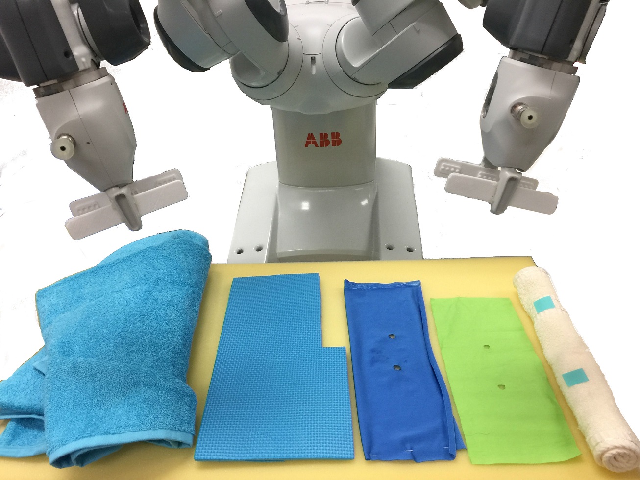
Figure 4: The set of deformable objects to be manipulated in our experiment. From left to right: towel, plastic sheet, stretchable fabric, unstretchable fabric, and rolled towel.

We evaluate our approach using one dual-arm robot (ABB Yumi) with 7 degrees-of-freedom in each arm. To get precise information of the 3D object to be manipulated, we set up a vision system including two 3D cameras with different perception fields and precision: one realsense SR300 camera for small objects and one ZR300 camera for large objects. The entire manipulation system is shown in Figuree 1. For FO-GPR parameters, we set the observation noise $\sigma_{n}=0.001$, the RBF spread width $\sigma_{RBF}=0.6$, and the maximum size of the Gram matrix $M=300$. The executing rate of our approach is $30$ FPS.

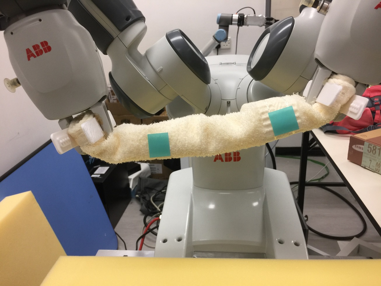
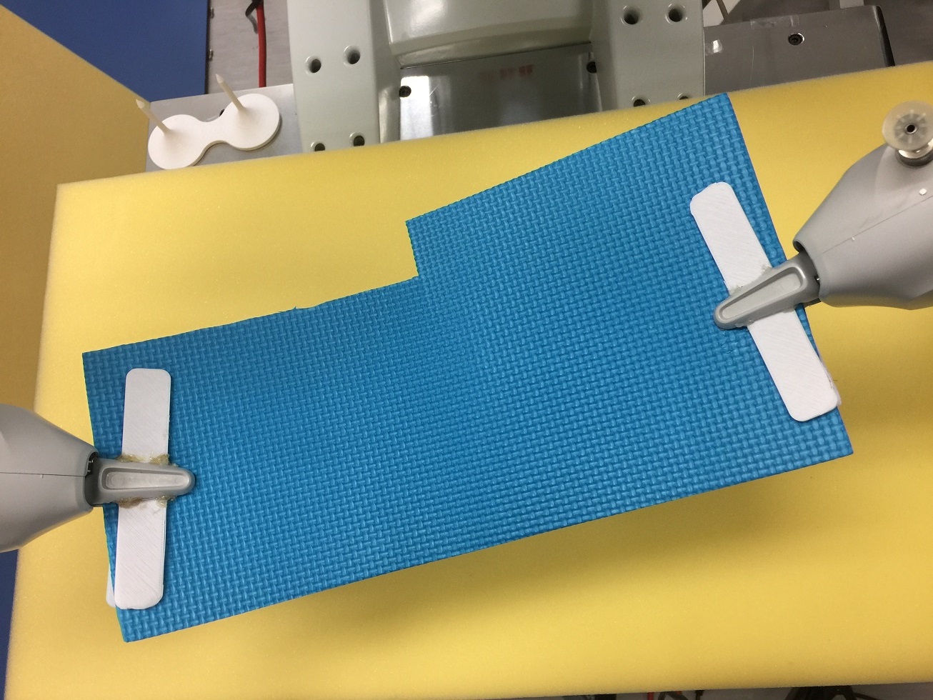
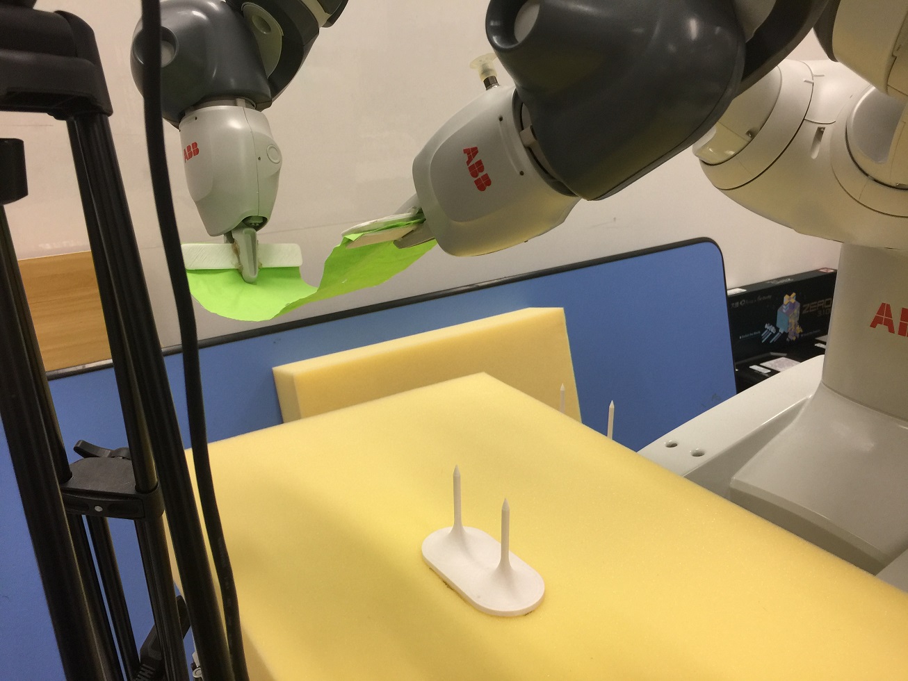
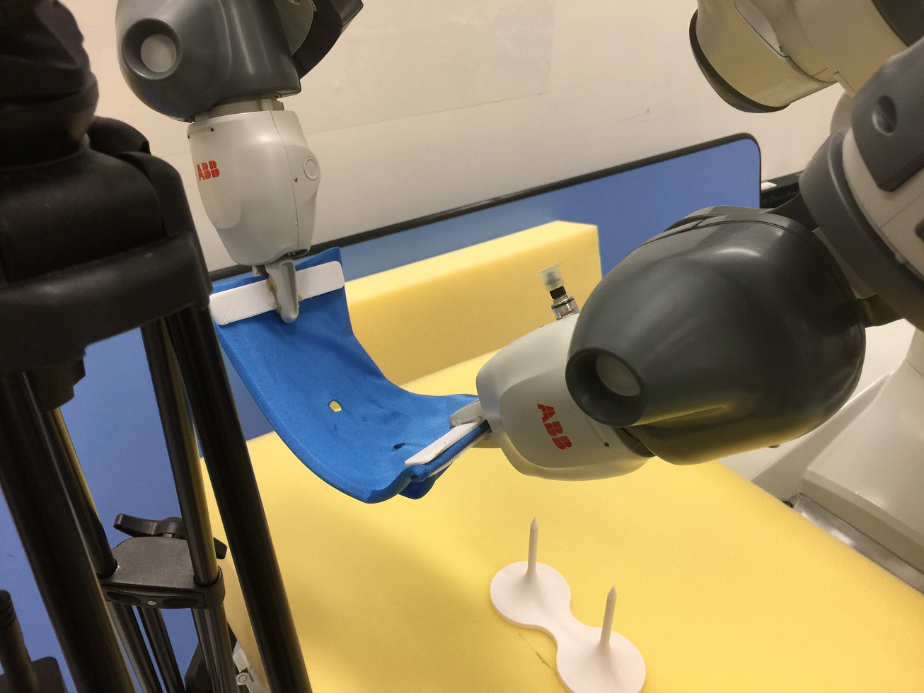
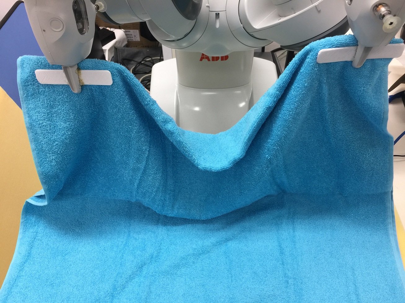
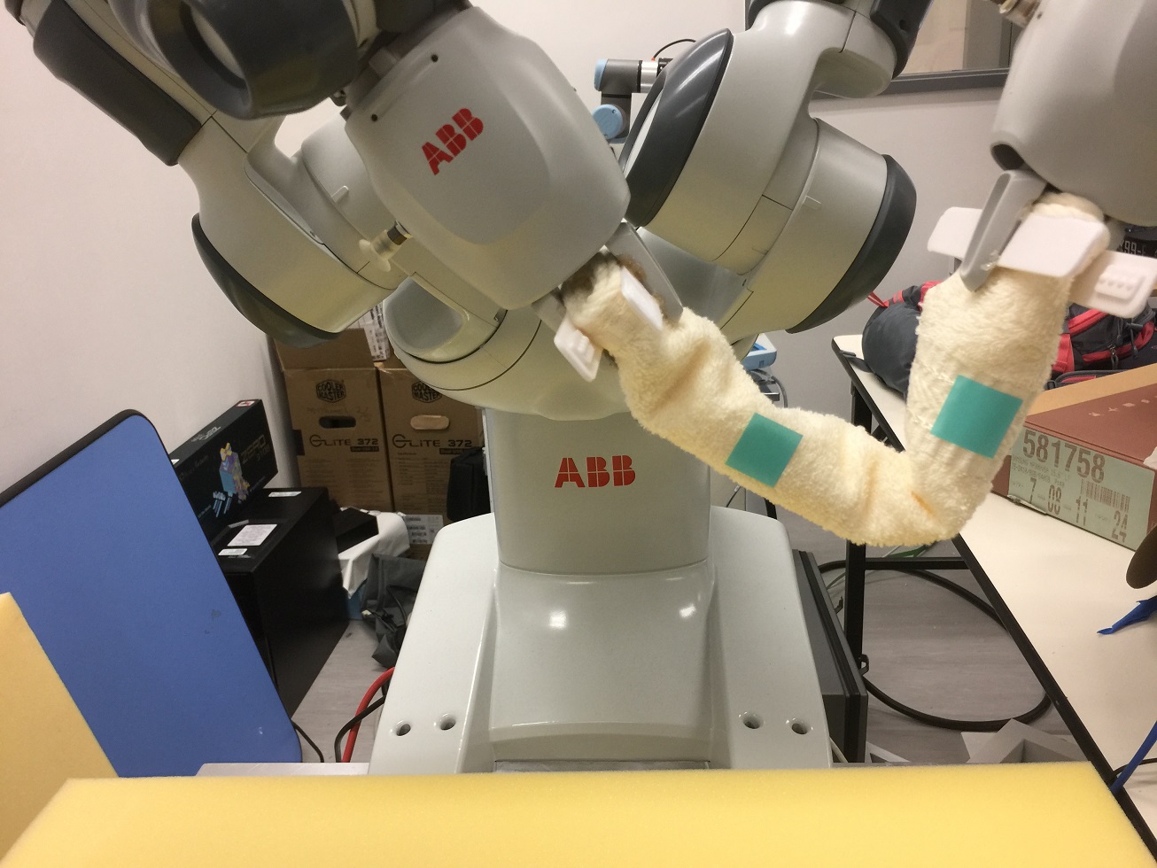
(a)

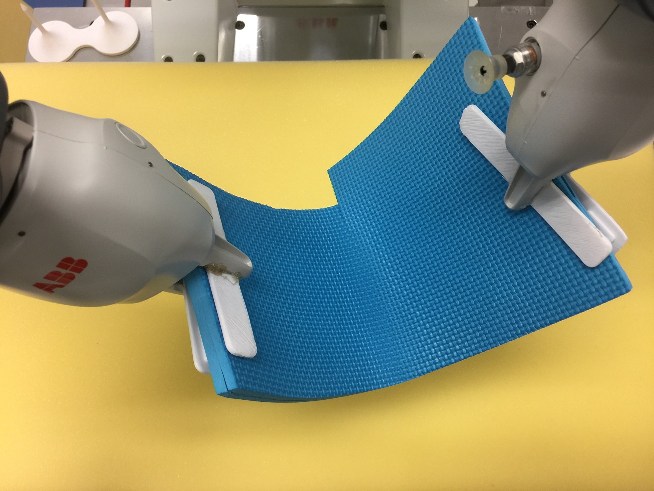
(b)

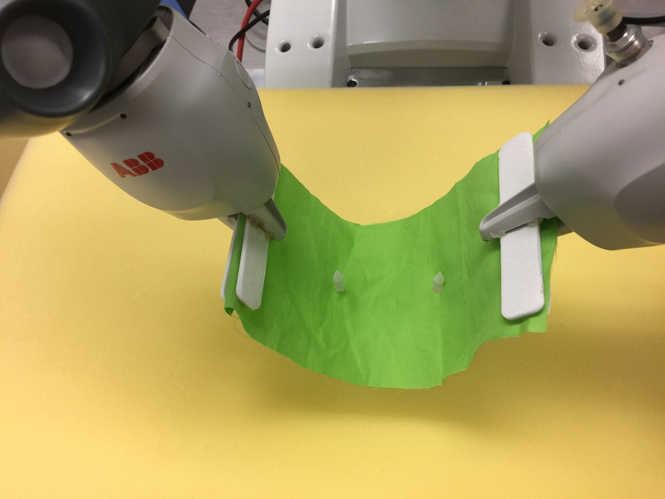
(c)

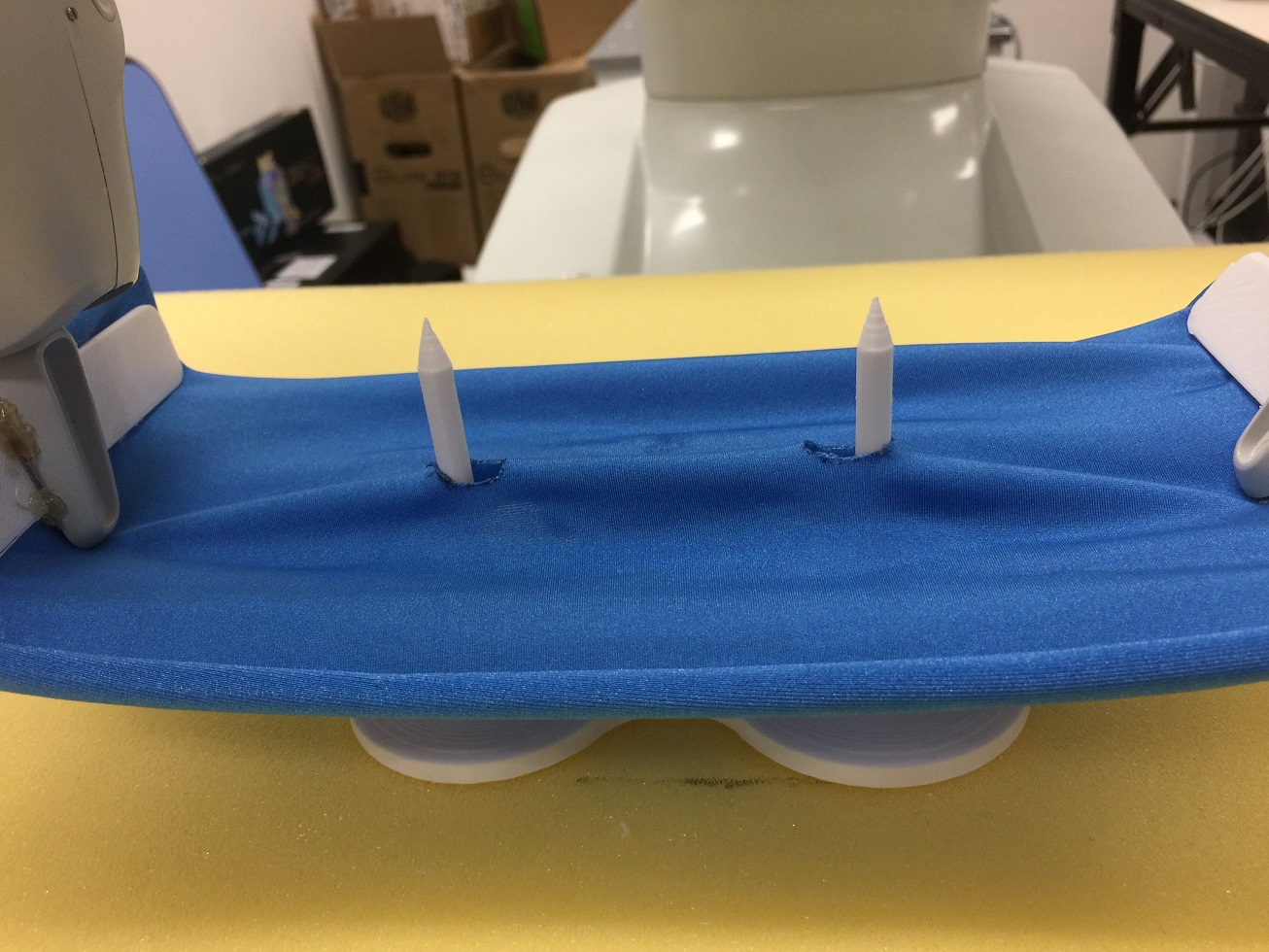
(d)

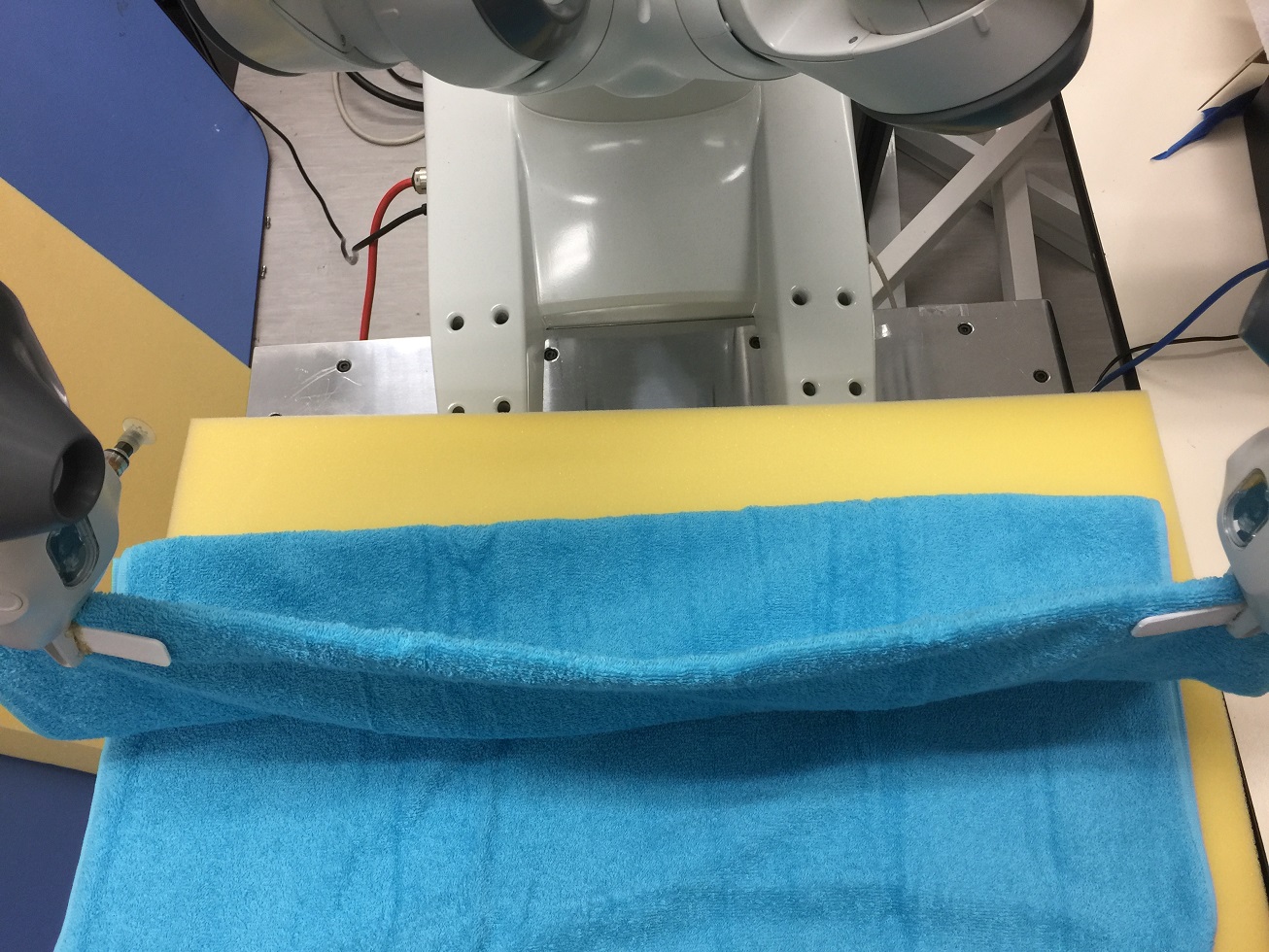
(e)

Figure 5: The set of tasks used to evaluate the performance of our approach: (a) rolled towel bending, (b) plastic sheet bending, (c) peg-in-hole for unstretchable fabric, (d) peg-in-hole for stretchable fabric, and (e) towel folding. The first row shows the initial state of each object before the manipulation and the second row shows the goal states of the object after the successful manipulation.

VI-B Manipulation Tasks

To evaluate the performance of our approach, we apply it to different manipulation tasks involving distinct objects as shown in Figure 4. For each task, we choose different set of features as discussed in Section V to achieve the best performance.

VI-B1 Rolled towel bending

This task aims at bending a rolled towel in to a specific goal shape as shown in Figure 5(a). We use a $4$-dimension feature vector $\mathbf{x}=\left[\mathbf{c},d\right]$ as the feature vector used in the FO-GPR driven visual-servo, where $\mathbf{c}$ is the centroid feature described by Equation 18 and $d$ is the distance feature as described by Equation 20 for two feature points on the towel.

VI-B2 Plastic sheet bending

This goal of this task is to manipulate a plastic sheet into a preassigned curved status as shown in Figure 5(b). We use a $4$-dimension feature vector $\mathbf{x}=\left[\mathbf{c},\sigma\right]$ to describe the state of the plastic sheet, where $\mathbf{c}$ is the centroid feature described by Equation 18 and $\sigma$ is the surface variation feature computed by Equation 22.

VI-B3 Peg-in-hole for fabrics

This task aims at moving cloth pieces so that the pins can be inserted into the corresponding holes on the fabric. Two different types of fabric with different stiffness have been tested in our experiment: one is an unstretchable fabric as shown in Figure 5(c) and the other is a stretchable fabric as shown in Figure 5(d). The $6$-dimension feature vector $\mathbf{x}=\mathbf{\rho}$ is the position of feedback points as described in Equation 19.

VI-B4 Towel folding

This task aims at flattening and folding a towel into a desired state as shown in Figure 5(e). We use a binned histogram of extended FPFH to describe the towel’s shape. The three values $\cos(\alpha)$, $\cos(\varphi)$ and $\theta$ are computed for all the feedback points using Equation 24, and are then aggregated into $45$ bins individually, generating a feature vector of $135$ dimensions. Since the feature has a very large dimension, for this experiment we need to manually move the robot in the beginning to explore sufficient data so that the FO-GPR can learn a good enough initial model for the complex deformation function.

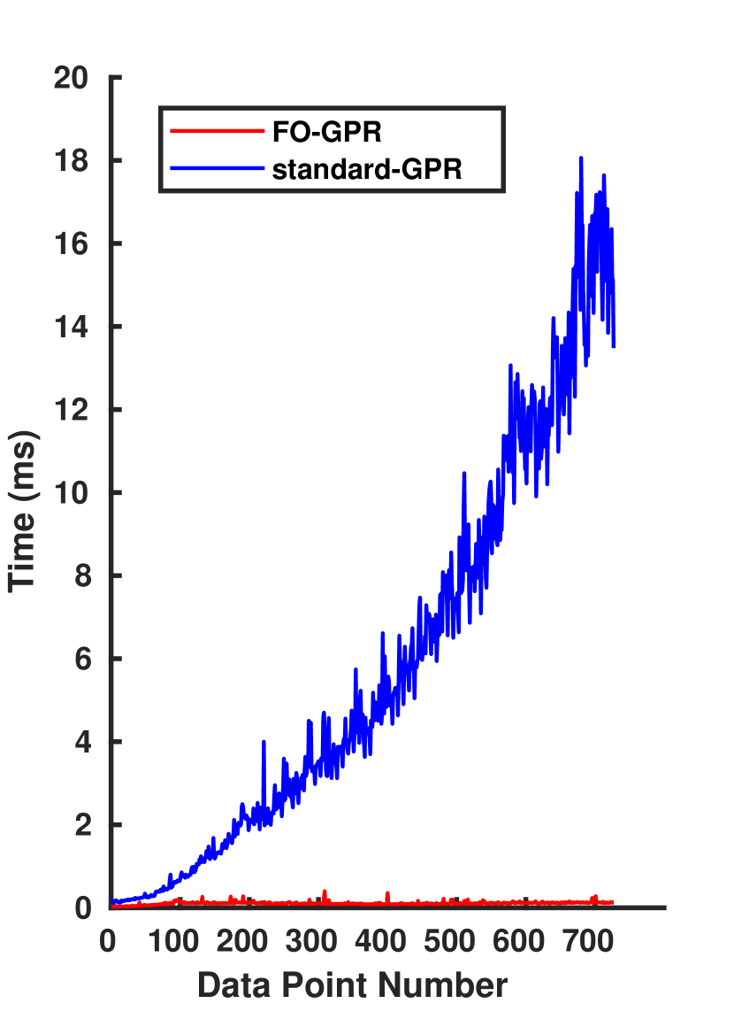
(a)

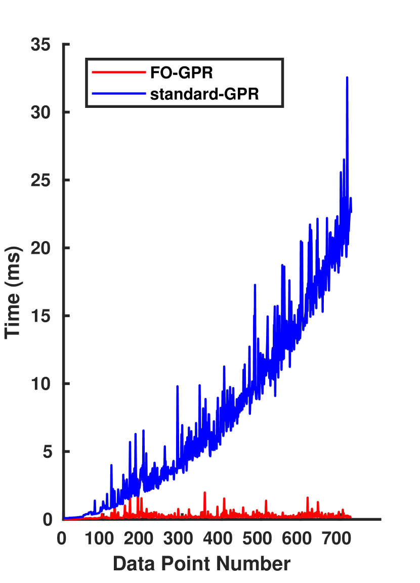
(b)

Figure 6: Comparison of the time cost of FO-GPR and standard GPR: (a) the time cost comparison between GP model estimation; (b) the time cost comparison for the entire manipulation process.

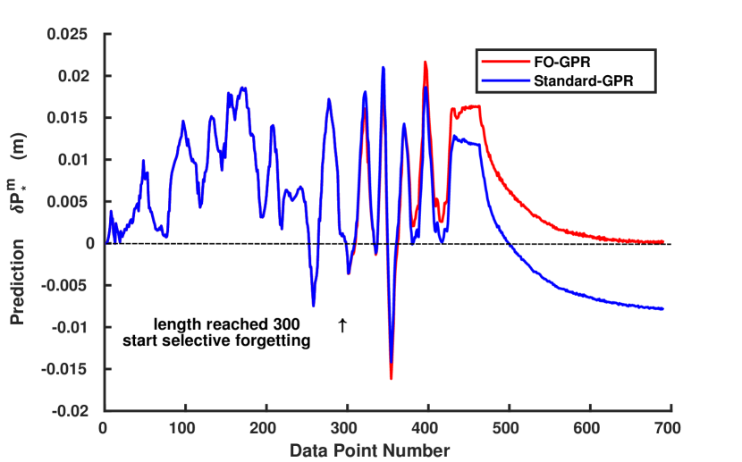
Figure 7: Impact of selective forgetting in FO-GPR: FO-GPR is superior over the standard GPR in terms of the computational cost and the deformation model accuracy.

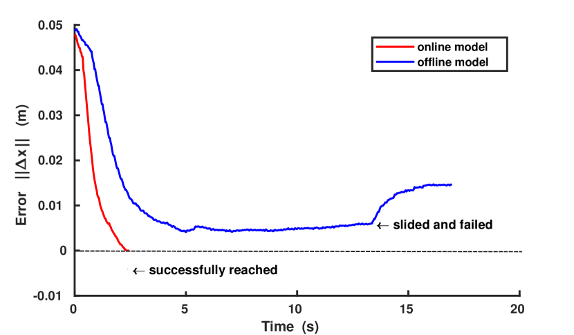
Figure 8: Comparison of online and offline GP models for rolled towel manipulation. The controller based on the online model succeeds while the controller based on the offline model fails.

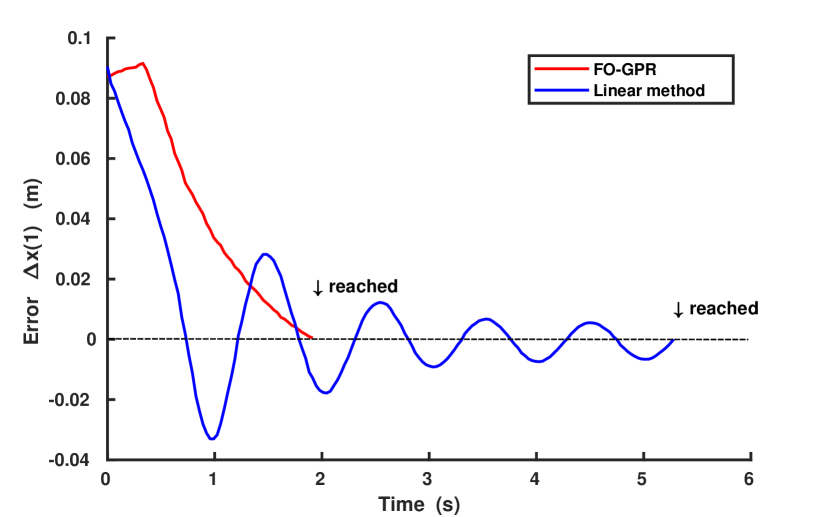
Figure 9: Comparison of the controllers based on FO-GPR and the linear model on the rolled towel task.

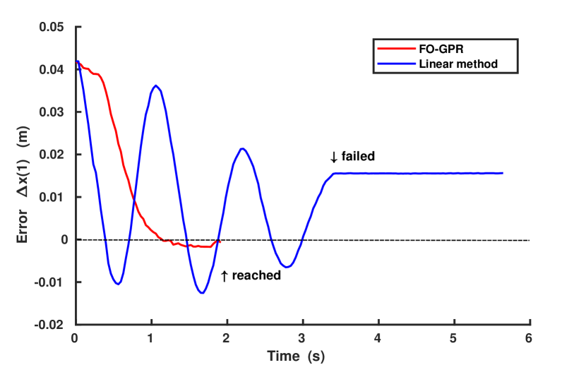
Figure 10: Comparison of the controllers based on FO-GPR and the linear model on the peg-in-hole task with stretchable fabric.

VI-C Results and Discussion

Our FO-GPR based manipulation control is able to accomplish all the five tasks efficiently and accurately. Please refer to the videos at https://sites.google.com/view/mso-fogpr for manipulation details.

Next, we provide some quantitative analysis of our approach by comparing with some state-of-the-art approaches.

VI-C1 Comparison of computational cost with standard GPR

As shown in Figure 6(a), the time cost of the standard GPR operation in each iteration increases significantly when the number of training points increases, which makes the online deformation function update impossible. Our FO-GPR method’s time cost is always under $2$ ms. We also compare the time cost of each complete cycle of the manipulation process, including feature extraction, tracking, robot control, and GPR, and the result is shown in Figure 6(b). Again, the time cost of manipulation using standard GPR fluctuates significantly, which can be 10 times slower than our FO-GPR based manipulation, whose time cost is always below $5$ ms and allows for real-time manipulation. This experiment is performed using the rolled towel bending task.

VI-C2 Impact of selective forgetting

In Figure 7, we compares the GP prediction quality between FO-GPR and the standard GPR on the rolled towel task, in order to show the impact of selective forgetting in FO-GPR. We record about $700$ data entries continuously. The first $450$ data are produced using random controller, and the rest are generated by the FO-GPR based controller which drives the soft object toward the target state smoothly. Before the data size reaches the maximum limit $M=300$, the controllers using two GPR models provide the same velocity output. From this point on, FO-GPR selectively forgets uninformative data while the standard GPR still uses all data for prediction. For data points with indices between $300$ and $450$, the output from two controllers are similar , which implies that FO-GPR still provides a sufficiently accurate model. After that, the FO-GPR based controller drives the object toward goal and eventually the controller output is zero; while for standard GPR, the controller output remains unzero. This experiment suggests that the performance of FO-GPR is much better than the GPR in real applications in terms of both time saving and the accuracy of the learned deformation model.

VI-C3 Comparison of online and offline GPR

In this experiment, we fix the Gram matrix unchanged after a while in the rolled towel manipulation task, and compare the performance of the resulting offline model with that of our online learning approach. As shown in Figure 8, the error in the feature space $\|\Delta\mathbf{x}\|_{2}$ decreases at the beginning of manipulation while using both models for control. However, when the soft object is close to its target configuration, the controller using the offline model cannot output accurate prediction due to the lack of data around the unexplored target state. Thanks to the balance of exploration and exploitation of online FO-GPR, our method updates the deformation model all the time and thus is able to output a relative accurate prediction so that the manipulation process is successful.

VI-C4 Comparison of FO-GPR and linear model

We compare our approach to the state-of-the-art online learning method for soft objects’ manipulation [16], which uses a linear model for the deformation function. First, we first through the experiment that the learning rate of the linear model has a great impact on the manipulation performance and needs to be tuned offline for different tasks; while our approach is able to use the same set of parameters for all tasks. Next, we perform both methods on the rolled towel and the peg-in-hole with stretchable fabric tasks, and the results are shown in Figure 9 and 10, respectively. To visualize the comparison results, we choose one dimension from the feature vector $\mathbf{x}$ and plot it. In Figure 9, we observe that the error of the controller based on the linear model decreases quickly, but the due to the error in other dimensions the controller still outputs a high control velocity and thus vibration starts. The controller needs a long time to accomplish the task. As a contrast, the error of the plotted dimension decreases slower but the controller finishes the task faster because the error of all dimensions declines to zero quickly, thanks to the nonlinear modeling capability of GPR. In the peg-in-hole task, we can observe that the GPR-based controller successfully accomplish the task while the controller based on the linear model fails.

VII Conclusion and Limitations

In this paper, we have presented a general approach to automatically servo-control soft objects using a dual-arm robot. We proposed an online GPR model to estimate the deformation function of the manipulated objects, and used low-dimension features to describe the object’s configuration. The resulting GPR-based visual servoing system can generate high quality control velocities for the robotic end-effectors and is able to accomplish a set of manipulation tasks robustly.

For future work, we plan to find a better exploration method to learn a more complicate deformation function involving not only the feature velocity but also the current configuration of the object in the feature space, in order to achieve more challenging tasks like cloth folding.

References

- [1] S. Miller, J. van den Berg, M. Fritz, T. Darrell, K. Goldberg, and P. Abbeel, “A geometric approach to robotic laundry folding,” The International Journal of Robotics Research, vol. 31, no. 2, pp. 249–267, 2011.
- [2] M. Cusumano-Towner, A. Singh, S. Miller, J. F. O’Brien, and P. Abbeel, “Bringing clothing into desired configurations with limited perception,” in IEEE International Conference on Robotics and Automation, 2011, pp. 3893–3900.
- [3] W. Wang, D. Berenson, and D. Balkcom, “An online method for tight-tolerance insertion tasks for string and rope,” in IEEE International Conference on Robotics and Automation, 2015, pp. 2488–2495.
- [4] D. Kruse, R. J. Radke, and J. T. Wen, “Collaborative human-robot manipulation of highly deformable materials,” in IEEE International Conference on Robotics and Automation, 2015, pp. 3782–3787.
- [5] S. Patil and R. Alterovitz, “Toward automated tissue retraction in robot-assisted surgery,” in IEEE International Conference on Robotics and Automation, 2010, pp. 2088–2094.
- [6] J. Schulman, J. Ho, C. Lee, and P. Abbeel, “Generalization in robotic manipulation through the use of non-rigid registration,” in International Symposium on Robotics Research, 2013.
- [7] L. Twardon and H. Ritter, “Interaction skills for a coat-check robot: Identifying and handling the boundary components of clothes,” in IEEE International Conference on Robotics and Automation, 2015, pp. 3682–3688.
- [8] D. Hadfield-Menell, A. X. Lee, C. Finn, E. Tzeng, S. Huang, and P. Abbeel, “Beyond lowest-warping cost action selection in trajectory transfer,” in IEEE International Conference on Robotics and Automation, 2015, pp. 3231–3238.
- [9] T. Tang, C. Liu, W. Chen, and M. Tomizuka, “Robotic manipulation of deformable objects by tangent space mapping and non-rigid registration,” in IEEE/RSJ International Conference on Intelligent Robots and Systems, 2016, pp. 2689–2696.
- [10] P. C. Yang, K. Sasaki, K. Suzuki, K. Kase, S. Sugano, and T. Ogata, “Repeatable folding task by humanoid robot worker using deep learning,” IEEE Robotics and Automation Letters, vol. 2, no. 2, pp. 397–403, 2017.
- [11] Y. Li, Y. Yue, D. Xu, E. Grinspun, and P. K. Allen, “Folding deformable objects using predictive simulation and trajectory optimization,” in IEEE/RSJ International Conference on Intelligent Robots and Systems, 2015, pp. 6000–6006.
- [12] Y. Li, D. Xu, Y. Yue, Y. Wang, S. F. Chang, E. Grinspun, and P. K. Allen, “Regrasping and unfolding of garments using predictive thin shell modeling,” in IEEE International Conference on Robotics and Automation, 2015, pp. 1382–1388.
- [13] D. McConachie and D. Berenson, “Bandit-based model selection for deformable object manipulation,” in Workshop on the Algorithmic Foundations of Robotics, 2016.
- [14] L. Bodenhagen, A. R. Fugl, A. Jordt, M. Willatzen, K. A. Andersen, M. M. Olsen, R. Koch, H. G. Petersen, and N. Krüger, “An adaptable robot vision system performing manipulation actions with flexible objects,” IEEE Transactions on Automation Science and Engineering, vol. 11, no. 3, pp. 749–765, 2014.
- [15] D. Navarro-Alarcon, Y. H. Liu, J. G. Romero, and P. Li, “Model-free visually servoed deformation control of elastic objects by robot manipulators,” IEEE Transactions on Robotics, vol. 29, no. 6, pp. 1457–1468, 2013.
- [16] D. Navarro-Alarcon, H. M. Yip, Z. Wang, Y. H. Liu, F. Zhong, T. Zhang, and P. Li, “Automatic 3-d manipulation of soft objects by robotic arms with an adaptive deformation model,” IEEE Transactions on Robotics, vol. 32, no. 2, pp. 429–441, 2016.
- [17] J. D. Langsfeld, A. M. Kabir, K. N. Kaipa, and S. K. Gupta, “Online learning of part deformation models in robotic cleaning of compliant objects,” in ASME Manufacturing Science and Engineering Conference, vol. 2, 2016.
- [18] D. Henrich and H. Wörn, Robot manipulation of deformable objects. Springer Science & Business Media, 2012.
- [19] M. Saha and P. Isto, “Manipulation planning for deformable linear objects,” IEEE Transactions on Robotics, vol. 23, no. 6, pp. 1141–1150, 2007.
- [20] M. Moll and L. E. Kavraki, “Path planning for deformable linear objects,” IEEE Transactions on Robotics, vol. 22, no. 4, pp. 625–636, 2006.
- [21] Y. Bai, W. Yu, and C. K. Liu, “Dexterous manipulation of cloth,” Computer Graphics Forum, vol. 35, no. 2, pp. 523–532, 2016.
- [22] T. Matsuno, D. Tamaki, F. Arai, and T. Fukuda, “Manipulation of deformable linear objects using knot invariants to classify the object condition based on image sensor information,” IEEE/ASME Transactions on Mechatronics, vol. 11, no. 4, pp. 401–408, 2006.
- [23] M. Bell and D. Balkcom, “Grasping non-stretchable cloth polygons,” International Journal of Robotics Research, vol. 29, no. 6, pp. 775–784, 2010.
- [24] A. Doumanoglou, J. Stria, G. Peleka, I. Mariolis, V. Petrík, A. Kargakos, L. Wagner, V. Hlaváč, T. K. Kim, and S. Malassiotis, “Folding clothes autonomously: A complete pipeline,” IEEE Transactions on Robotics, vol. 32, no. 6, pp. 1461–1478, 2016.
- [25] D. Berenson, “Manipulation of deformable objects without modeling and simulating deformation,” in IEEE/RSJ International Conference on Intelligent Robots and Systems, 2013, pp. 4525–4532.
- [26] S. Hirai and T. Wada, “Indirect simultaneous positioning of deformable objects with multi-pinching fingers based on an uncertain model,” Robotica, vol. 18, no. 1, pp. 3–11, 2000.
- [27] E. Snelson and Z. Ghahramani, “Sparse gaussian processes using pseudo-inputs,” in Advances in neural information processing systems, 2006, pp. 1257–1264.
- [28] C. E. Rasmussen and Z. Ghahramani, “Infinite mixtures of gaussian process experts,” in Advances in neural information processing systems, 2002, pp. 881–888.
- [29] E. Snelson and Z. Ghahramani, “Local and global sparse gaussian process approximations,” in Artificial Intelligence and Statistics, 2007, pp. 524–531.
- [30] D. Nguyen-Tuong, J. R. Peters, and M. Seeger, “Local gaussian process regression for real time online model learning,” in Advances in Neural Information Processing Systems, 2009, pp. 1193–1200.
- [31] R. B. Rusu, N. Blodow, and M. Beetz, “Fast point feature histograms (fpfh) for 3d registration,” in IEEE International Conference on Robotics and Automation, 2009, pp. 1848–1853.