Sensitivity of Displacement Detection for a Particle Levitated in the Doughnut Beam

Abstract

Displacement detection of a sphere particle in focused laser beams with quadrant photodetector (QPD) provides a fast and high precision way to determine the particle location. In contrast to the traditional Gaussian beams, the sensitivity of displacement detection using various doughnut beams are investigated. The sensitivity improvement for large sphere particles along the longitudinal direction is reported. With appropriate vortex charge $l$ of the doughnut beams, they can outperform the Gaussian beam to get more than one order higher sensitivity and thus have potential applications in various high precision measurement. By using the levitating doughnut beam itself to detect the particle displacement, the result will also facilitate the recent proposal of levitating a particle in doughnut beams to suppress the light absorption.

Introduction The displacement of the levitated particle is usually measured by the interferometry method with quadrant photodetector (QPD) in the back focal plane Denk and Webb (1990); Svoboda et al. (1993); Finer et al. (1994); Gittes and Schmidt (1998); Pralle et al. (1999); Rohrbach and Stelzer (2002); Rohrbach et al. (2003); Volpe et al. (2007). With high sensitivity and high bandwidth, it is widely used in high precision displacement measurement Denk and Webb (1990), weak force measurement Svoboda et al. (1993); Finer et al. (1994), photon force microscope Florin et al. (1997), optical nanoprobing Rodríguez-Herrera et al. (2010) and even surface imaging Friedrich and Rohrbach (2015). Especially, with the sensitivity as high as 3 $\rm{fm/\sqrt{Hz}}$ Li (2012), it can measure the instantaneous velocity of brownian particle Li et al. (2010); Li (2012) and provides a key tool to investigate the dynamics of the particle in various physical systems Mazilu et al. (2016); Jiang et al. (2010) including the optomechanical system Neukirch et al. (2015); Hoang et al. (2016).

Particle levitated by laser beam absorbs light and meets heating problem Neukirch et al. (2015); Hoang et al. (2016). It is proposed to reduce heating of strong absorptive particle by designing a core-shell structure of the particle and trapping it in the doughnut-shaped beams Zhou et al. (2017). The proposal of the using doughnut beams show excellent tolerance of the heat absorption of the particle and keeps the high quality factor of the mechanical oscillation. When the laser beam is changing from Gaussian beam to doughnut beams, it is significant to know how the doughnut beams affect the sensitivity in detecting the particle displacement.

The interferometry method with QPD has been investigated extensively using Gaussian beam Denk and Webb (1990); Svoboda et al. (1993); Finer et al. (1994); Gittes and Schmidt (1998); Pralle et al. (1999); Rohrbach and Stelzer (2002); Rohrbach et al. (2003); Volpe et al. (2007); Friedrich and Rohrbach (2015). However, few papers have investigated the sensitivity of displacement detection of a particle in doughnut beams van de Nes and Torok (2007); Garbin et al. (2008, 2009). Nes et. al. van de Nes and Torok (2007) has investigated the scattering of a sphere particle in LG beam and shown the response signal of QPD for certain LG beams. Garbin et. al. Garbin et al. (2009) have investigated the signal of QPD for LG beams with different sign of vortex charge $l$. It has shown that the result can be used to distinguish the vortex charge of the beam. Here, we give a detail and systematical investigation of interferometry method using various doughnut beams. Especially, the displacement detection with the large sphere particle size has been included. The result shows that the interferometry method is still efficient for doughnut beams. More importantly, the sensitivity along the longitudinal direction is dramatically improved for large sphere particles. By choosing appropriate doughnut beams, they can outperform the Gaussian beam with more than one order.

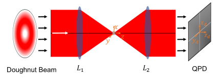
Figure 1: The schematic of the displacement detection setup in an optical levitating system (consisted of an optical trap and a trapped particle). Incident beams here include various doughnut beams. The field after the particle scattering is collected by lens ${\rm L}_{2}$ to the quadrant photodetector (QPD) to get the signal.

The system structure and method The system we considered is shown in Fig. 1. The incident laser beam is focused by a high Numerical Aperture (NA) objective lens ${\rm L}_{1}$ to trap a sphere particle near the focus in vacuum. The scattering beam field, along with the incident beam field is collected by the second lens ${\rm L}_{2}$ to the QPD as the detection signal. In the previous literatures Gittes and Schmidt (1998); Pralle et al. (1999); Rohrbach and Stelzer (2002); Rohrbach et al. (2003); Volpe et al. (2007), the incident beam is typically Gaussian beam. Here we focused on various doughnut beams. The system is described with the following parameters: the power of incident beam $P$, the wavelength of the beam in vacuum $\lambda_{0}$, the polarization of incident beam $\mathbf{e}$, the numerical aperture of the object lens ${\rm NA}$, the filling factor of the incident beam $f_{01}$ and the radius of sphere particle $a$. Unless stated otherwise, we assume $P=100\ {\rm mW}$, $\lambda_{0}=1064\ {\rm nm}$, ${\rm NA}=0.95$, $\mathbf{e}=\mathbf{\hat{\mathbf{x}}}$ and $f_{01}=1.0$ in this work.

We apply the generalized Lorentz-Mie Theory (GLMT) to simulate the electromagnetic field scattering by the particle. The GLMT has been widely used in literatures Nieminen et al. (2007); Chen et al. (2009), and provides a powerful and convenient tool to calculated the scattering field. In this method, the incident and scattering beam are described by the partial wave expansion coefficients in the bases of vector spherical wave functions. The two sets of coefficients are linked by the $T$-Matrix of the particle which is independent of the incident beam. The strongly focused incident beam cannot be described by the expression of paraxial beam, thus we described the beam by the generalized vector Debye integral theory Chen et al. (2009).

The incident and scattered electromagnetic fields are collected by the lens ${\rm L}_{2}$. The QPD then outputs the response signal based on the interference distribution of the light intensity. The responses signals of the QPD are Jones et al. (2015)

$$S_{x} = \underset{x_{d}>0}{\iint}I(x_{d},y_{d})dx_{d}dy_{d}-\underset{x_{d}<0}{\iint}I(x_{d},y_{d})dx_{d}dy_{d},$$ (1a)

$$S_{y} = \underset{y_{d}>0}{\iint}I(x_{d},y_{d})dx_{d}dy_{d}-\underset{y_{d}<0}{\iint}I(x_{d},y_{d})dx_{d}dy_{d},$$ (1b)

$$S_{z} = \iint I(x_{d},y_{d})dx_{d}dy_{d}.$$ (1c)

Among Eqs. (1a-1c), the subscripts $x,y,z$ denote the QPD’s three different signals respectively. Usually, $S_{x}$ is chosen to measure the particle displacement for a particle moving along the $x$ direction for example, because the signal $S_{x}$ changes most dramatically at the same time. So are the cases of $S_{y}$ and $S_{z}$. Since both $S_{x}$ and $S_{y}$ denote the signals in the transverse direction and have similar behaviors, we mainly show the results of $S_{x}$ and $S_{z}$ in the investigation below without loss of generality. The light intensity on the detector is $I(x_{d},y_{d})=\frac{c\varepsilon_{d}}{2n_{d}}|\mathbf{E}(x_{d},y_{d})|^{2}$, where the permittivity and refractive index of medium before the detector are $\varepsilon_{d}$ and $n_{d}$ respectively. The velocity of light in vacuum is denoted as $c$. The field $\mathbf{E}(x_{d},y_{d})$ is the electric field on the detector. It can be written as $\mathbf{E}(x_{d},y_{d})={\mathbf{E}_{\rm inc}}(x_{d},y_{d})+{\mathbf{E}_{\rm scat}}(x_{d},y_{d})$, where ${\mathbf{E}_{\rm inc}}(x_{d},y_{d})$ comes from the incident beam which can be expressed analytically for the confocal system here; and ${\mathbf{E}_{\rm scat}}(x_{d},y_{d})$ comes from the scattering filed, which is calculated through the $T$-matrix method.

Result In this part, we show the numerical result of displacement detection sensitivity for a particle in Gaussian beam, and various doughnut beams. The definition of doughnut beams including LG beam with different vortex charge $l$, radially polarized and azimuthally polarized beam follows the convention in Ref. Jones et al. (2015).

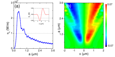
Figure 2: (a) The sensitivity of displacement detection using QPD for a silica sphere particle trapped in the $\hat{\mathbf{x}}$ direction linearly polarized Gaussian beam. The inset: a typical response of the QPD for a sphere particle ($a=400\ {\rm nm}$) moving along the x axis in the Gaussian beam. (b) The response signal of the QPD for particles with various radii in the $\hat{\mathbf{x}}$ direction linearly polarized Gaussian beam.

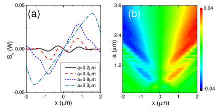
Figure 3: (a) The typical response of the QPD for a silica particle particle moving along the x axis in the $\hat{\mathbf{x}}$ direction linearly polarized ${\rm LG}_{01}$ beam. Cases with some representative particle radii have been shown. The slope near the beam focus (i.e., the sensitivity) could be either positive or negative. (b) The response signal of the QPD for particles with various radii in the $\hat{\mathbf{x}}$ direction linearly polarized ${\rm LG}_{01}$ beam.

Sensitivity and Range of a sphere particle in Gaussian beam Figure 2(a) shows the result of the detection sensitivity using Gaussian beam, for a silica sphere particle moving along $\hat{\mathbf{x}}$ direction in vacuum. Especially, the case for the sphere particle with large size (i.e., much larger than the wavelength) is included. In the inset of Fig. 2(a), the response signal of the QPD for a sphere with radius $a=0.4\ \upmu{\rm m}$ is shown. The sensitivity is defined as

$$\left.\eta_{i}=\frac{dS_{i}}{dr_{i}}\right|_{\mathbf{r}=\mathbf{r}_{0}},$$ (2)

where $i=x,y,z$ denote the sensitivity along different displacement direction and ${\mathbf{r}_{0}}$ is the location of the particle. Here we focus on ${\mathbf{r}_{0}}=0$ in the work because the sensitivity usually reaches it best at the axis origin. As shown in Fig. 2(a), the sensitivity $\eta$ increase with the increasing sphere particle radius $a$ and reaches the maximum when $a\approx 0.4\ \upmu{\rm m}$. At this point, the particle size is comparable with the beam waist. With larger radius $a$, the sensitivity decreases and shows shallow modulations. The shallow modulations in the sensitivity curve when $a>0.4\ \upmu{\rm m}$ are caused by the Mie resonance which changes the scattering field distribution.

Sensitivity of a particle in doughnut beams The QPD signal of a sphere particle in LG beams is quite different from that in Gaussian beam. As shown in Fig. 3(a), taking the ${\rm LG}_{01}$ beam as an example, there are more maximums and minimums of the signal $S_{x}$ when the particle location changes. The slope of $S_{x}$ about $x$ at the coordinate origin, which is defined as sensitivity, could be either positive or negative depending on the radius $a$. Figure 4(a) shows the result of the sensitivity $\eta_{x}$ for ${\rm LG}_{0l}$ beams with $l=1,2,3$. The sensitivity for Gaussian beam (i.e., $l=0$) is also shown for comparison. For particles with size $a$ much larger than the beam waist size, the sensitivity of LG beams show the same behavior with that of Gaussian beam. However, for $a$ smaller than the beam waist size, the sensitivity of LG beams (taking ${\rm LG}_{01}$ beam as an example) will change from negative to positive at certain size $R_{0}$. The displacement direction can be positive or negative when the response signal is positive, depending on whether the size of the particle exceeds $R_{0}$. This is different from that in Gaussian beam (blue solid line), which is always positive.

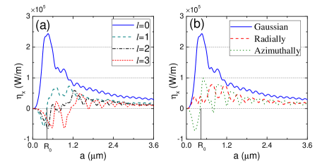
Figure 4: (a) The sensitivity of the transverse displacement detection for different particle radii in the $\hat{\mathbf{x}}$ direction linearly polarized ${\rm LG}_{01}$, ${\rm LG}_{02}$ and ${\rm LG}_{03}$ beam and Gaussian beam (i.e., $l=0$). (b) The same as Fig. (a) for radially and azimuthally polarized beams.

The different behaviors here are caused by the doughnut shape of intensity distribution of LG beams. The scattering field will show totally different distribution depending on two factors. One is whether the particle is inside or outside the bright rings of LG beams. The other one is whether the particle radius is larger than the size of the bright rings. To show this more clearly, the QPD signal $S_{x}$ are plotted with various sphere radii and locations in Fig. 3(b) and Fig. 2(b) for linearly polarized ${\rm LG}_{01}$ beam and Gaussian beam, respectively. For the ${\rm LG}_{01}$ beam, the QPD signal shows different behaviors when the particle size is smaller than the beam waist size. There are more lobes which affect the sensitivity.

For Gaussian beam, the sensitivity increases first and then decreases with the increasing size of the sphere particle, and there is a tradeoff between the sensitivity and linear range of displacement detection. It is the same for LG beams only when the particle size is larger than the beam waist size. For smaller particles in LG beams, as the sensitivity sign depends on the particle size and changes dramatically near $R_{0}$, it could be used to measure the size of particle with high accuracy. The sensitivity for radially and azimuthally polarized beams is shown in Fig. 4(b). The azimuthally polarized beam shows same behaviors as LG beams. The radially polarized beam shows similar behavior as the linearly polarized Gaussian beam, except the large modulations when the particle size is smaller than the beam waist size.

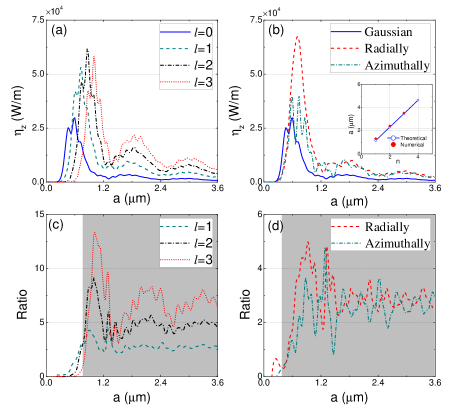
Figure 5: (a) The sensitivity $\eta_{z}$ of the longitudinal displacement detection, for different particle radii $a$ in the $\hat{\mathbf{x}}$ direction linearly polarized ${\rm LG}_{01}$, ${\rm LG}_{02}$ and ${\rm LG}_{03}$ beam and Gaussian beam (i.e., $l=0$). (b) The same as Fig. 5(a) for radially and azimuthally polarized beams. (c) The sensitivity improvement ratio $\xi$ for LG beams. (d) The same as Fig. 5(c) for radially and azimuthally polarized beams. The region is colored grey in Fig. 5(c) and Fig. 5(d) where the particle can be trapped stably by $\rm{LG_{03}}$ beam and azimuthally polarized beam respectively.

The sensitivity along longitudinal direction $\eta_{z}$ using various beams is shown in Fig. 5(a) and Fig. 5(b). Similar to the case for transverse displacement, the sensitivity increases first and then decreases with the increasing size of the sphere particle. With larger radius $a$, the sensitivity shows a large period oscillation along with shallow modulations. The shallow modulations is caused by the Mie resonance as in the transverse case. The large period oscillation is induced by the interference between the incident beam propagating directly to the detector and the scattering beam passing through the sphere particle to the detector. The destruction interference point is then given by

$$2ak_{0}(n_{m}-1)=2n\pi,$$ (3)

where $n$ are positive integers, $n_{m}=1.458$ is the refractive index of the silica sphere particle and $k_{0}$ is the vacuum wavevector. To verify this, minimum points for the case of Gaussian beam in Fig. 5(b) are plotted in its inset to compare with the theoretical result given by Eq. (3). Thus we also get the oscillation period

$$\lambda_{L}=\frac{\lambda_{0}}{2(n_{m}-1)},$$ (4)

and $\lambda_{L}=1.16\ \upmu{\rm m}$ here. The existence of these destruction interference point has a disadvantage in the displacement detection for sphere particles with size $a=n\lambda_{L}$.

At the same time, it is noticed that the sensitivity $\eta_{z}$ in doughnut beam is higher than that in Gaussian beam, when the size of the particle is comparable or lager than the beam waist. We define the sensitivity improvement ratio as

$$\xi_{l}=\eta_{\text{z},l}/\eta_{\text{z,Gaussian}},$$ (5)

where $l=1,2,3$ denotes different LG beams. The result is shown in Fig. 5(c). The improvement ratio of sensitivity can be more than one order. Especially, the grey region in Fig. 5(c) shows where the particle could be trapped stably by LG beams (taking the ${\rm LG}_{03}$ beam as an example) Zhou et al. (2017). The region of improved sensitivity (i.e., $\xi>1$) falls just into the grey region, thus the LG beam provides higher sensitivity in LG beam levitated systems. The sensitivity improvement ratio for radially and azimuthally polarized beams is shown in Fig. 5(d) and it has the same improvement behavior as LG beams.

Discussion It is significant to know the best sensitivity we could get for a particle with certain size. The systematically result for Gaussian beam and various doughnut beams here will facilitate us to choose the proper beam to get optimal sensitivity. Generally speaking, Gaussian beam will get better sensitivity for transverse displacement detection. However, doughnut beams can have one order higher sensitivity for longitude displacement detection, when the particle has the size exceeds the beam waist.

As a conclusion, the sensitivity of displacement detection of a particle in various doughnut beams are studied. We pay attention especially to the case of large particle size. The result for doughnut beams provides us the ability to choose proper beam to get best sensitivity. By using the levitating doughnut beam itself to detect the particle displacement, it will also benefit the recent proposal of levitating a particle using doughnut beams to suppress the light absorption.

Note: In the last version of this manuscript on arXiv, there was a mistake: the incident beam hasn’t been normalized to the power $P=100\ {\rm mW}$ while the scattering beam has. So, as the incident beam has the power of only several percent of the scattering beam power, the last version showed approximately the signal behaviors of scattering beams.

Acknowledgement We thank Prof. Zhi-Fang Lin and Dr. Wen-Zhao Zhang for the helpful discussion. This work is supported by Science Challenge Project No. TZ2018003, National Basic Research Program of China No. 2014CB848700, No. 2016YFA0301201, NSFC No. 11534002, NSAF U1730449 and NSAF No. U1530401. Z.-Q. Y. is supported by NSFC Grant 61771278, 61435007, and the Joint Fund of the Ministry of Education of China (6141A02011604). J.C. is supported by NSFC No. 11674204.

Appendix A Field on the detector

For the detection system described in the main text, it can be simplified as a confocal system as show in Fig. 6. The incident field ${\mathbf{E}_{\rm inc}}(x_{d},y_{d})$ on the detector is denoted as $\mathbf{E}_{4}(x,y,f_{2})$ here. It can be expressed by the incident filed $\mathbf{E}_{{\rm inc}}(x,y,-f_{1})$ as

$$\mathbf{E}_{4}(x_{2},y_{2},f_{2})=-e^{ik(f_{2}+f_{1})}e^{il\phi}\mathbf{E}_{{\rm inc}}(-\frac{x_{2}}{M},-\frac{y_{2}}{M},-f_{1}).$$ (6)

To make our convention clear, we will show the procedures to get this relation here.

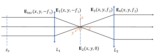
Figure 6: Theoretical model of the detection system. Here $\mathbf{E}_{{\rm inc}}(x,y,-f_{1})$ and $\mathbf{E}_{1}(x,y,-f_{1})$ are used to denote the field on the left and right side of the focusing lens $L_{1}$. Field $\mathbf{E}_{3}(x,y,f_{2})$ and $\mathbf{E}_{4}(x,y,f_{2})$ are used to denote the field on the left and right side of the collecting lens (condensor) $L_{2}$. And $\mathbf{E}_{2}(x,y,0)$ denotes the field on the $z=0$ plane.

A.1 Angular spectrum representation of a propagating wave

An electromagnetic field $\mathbf{E}(x,y,z)$ in the space satisfies the Maxwell equations. The electric field $\mathbf{E}(x,y,z\mathbf{)}$ can be expressed as

$$\mathbf{E}(x,y,z)=\stackrel{{\scriptstyle[}}{{-}}\infty]{\infty}{\iint}\mathbf{\hat{E}}(k_{x},k_{y};z)e^{i(k_{x}x+k_{y}y)}dk_{x}dk_{y},$$ (7)

where $\mathbf{\hat{\mathbf{E}}}(k_{x},k_{y};z)$ is the Fourier transform of the electrical field on the $z={\rm constant}$ plane $\mathbf{E}(x,y,z)$:

$$\mathbf{\hat{\mathbf{E}}}(k_{x},k_{y};z)=\frac{1}{4\pi^{2}}\stackrel{{\scriptstyle[}}{{-}}\infty]{\infty}{\iint}\mathbf{E}(x,y,z)e^{-i(k_{x}x+k_{y}y)}dxdy.$$ (8)

Considering the case that the medium in the space is source free, linear, homogeneous and isotropic, the $\mathbf{E}(x,y,z)$ satisfy the vector Helmholtz equation:

$$(\nabla^{2}+k^{2})\mathbf{E}(x,y,z)=0.$$ (9)

Substituting Eq. (7) into Eq. (9), we get the general solution (see similar materials on pp. 110 in Ref. Mandel and Wolf (1995))

$$\mathbf{\hat{E}}(k_{x},k_{y};z)=\mathbf{\hat{A}}(k_{x},k_{y})e^{ik_{z}z}+\mathbf{\hat{B}}(k_{x},k_{y})e^{-ik_{z}z},$$ (10)

where we define $k_{z}=(k^{2}-k_{x}^{2}-k_{y}^{2})^{\frac{1}{2}}$ and ${\rm Im}(k_{z})>0$. On substituting Eq. (10) into Eq. (7) the field

$$\mathbf{E}(x,y,z) = \stackrel{{\scriptstyle[}}{{-}}\infty]{\infty}{\iint}[\mathbf{\hat{A}}(k_{x},k_{y})e^{ik_{z}z}+\mathbf{\hat{B}}(k_{x},k_{y})e^{-ik_{z}z}]$$ (11)

$$\times e^{i(k_{x}x+k_{y}y)}dk_{x}dk_{y}.$$

It is noted that so far we haven’t specified the propagating direction of $\mathbf{E}(x,y,z)$ or any other physical information. In fact, $\mathbf{E}(x,y,z)$ expressed by Eq. (11) has four parts: homogeneous wave propagating in the positive $\mathbf{z}$ direction ($e^{ik_{z}z}$, $k_{x}^{2}+k_{y}^{2}<k^{2}$), evanescent wave propagating in the positive $\mathbf{z}$ direction ($e^{ik_{z}z}$, $k_{x}^{2}+k_{y}^{2}>k^{2}$), homogeneous wave propagating in the negative $\mathbf{z}$ direction ($e^{-ik_{z}z}$, $k_{x}^{2}+k_{y}^{2}<k^{2}$), and evanescent wave propagating in the negative $\mathbf{z}$ direction ($e^{-ik_{z}z}$, $k_{x}^{2}+k_{y}^{2}>k^{2}$).

Now we consider an electromagnetic wave propagating along positive $\mathbf{z}$ direction into the $z\geq z_{s}$ half space where $z_{s}\rightarrow-\infty$. First, since we have known the direction of the wave, then $B(k_{x},k_{y})=0$. Thus Eq. (10) is reduced to

$$\mathbf{\hat{E}}(k_{x},k_{y};z)=\mathbf{\hat{A}}(k_{x},k_{y})e^{ik_{z}z}.$$ (12)

Also, setting $z=0$ in Eq. (12) we get

$$\hat{\mathbf{A}}(k_{x},k_{y})=\mathbf{\hat{E}}(k_{x},k_{y};0),$$ (13)

where $\mathbf{\hat{\mathbf{E}}}(k_{x},k_{y};0)$ is the Fourier transform of the electrical field on the $z=0$ plane $\mathbf{E}(x,y,0)$:

$$\mathbf{\hat{\mathbf{E}}}(k_{x},k_{y};0)=\frac{1}{4\pi^{2}}\stackrel{{\scriptstyle[}}{{-}}\infty]{\infty}{\iint}\mathbf{E}(x,y,0)e^{-i(k_{x}x+k_{y}y)}dxdy.$$ (14)

Second, $\mathbf{\hat{E}}(k_{x},k_{y};z_{s})=\mathbf{\hat{E}}(k_{x},k_{y};0)e^{ik_{z}z_{s}}$ with $z_{s}\rightarrow-\infty$ should be a finite value when $k_{x}^{2}+k_{y}^{2}>k^{2}$, because it represents a physical field. Thus $\mathbf{\hat{E}}(k_{x},k_{y};0)=0$ when $k_{x}^{2}+k_{y}^{2}>k^{2}$. It means that a propagating wave has none evanescent part (saying in another way, the evanescent wave can’t propagate along the positive $\mathbf{z}$ direction to far from $z=z_{s}$). The electric field $\mathbf{E}(x,y,z\mathbf{)}$ in the $z\geq z_{s}$ half space with $|z-z_{s}|\gg 0$ now reads

$$\mathbf{E}(x,y,z)=\underset{k_{x}^{2}+k_{y}^{2}\leq k^{2}}{\iint}\mathbf{\hat{E}}(k_{x},k_{y};0)e^{i(k_{x}x+k_{y}y+k_{z}z)}dk_{x}dk_{y}.$$ (15)

A.2 Focusing of the propagating wave by aplanatic lens

As shown in Fig. 6, $\mathbf{E}_{{\rm inc}}(x,y,-f_{1})$ and $\mathbf{E}_{1}(x,y,-f_{1})$ are used to denote the field on the left and right side of the lens $L_{1}$. $\mathbf{E}_{3}(x,y,f_{2})$ and $\mathbf{E}_{4}(x,y,f_{2})$ are used to denote the field on the left and right side of the lens $L_{2}$. And $\mathbf{E}_{2}(x,y,0)$ denotes the field on the $z=0$ plane.

Using the stationary phase method Carter (1972); Mandel and Wolf (1995), Eq. (15) can be evaluated. For $z>0$ and $kr\rightarrow+\infty$, it reads

$$\mathbf{E}_{+\infty}(x,y,z)=-2\pi is_{z}k\mathbf{\hat{E}}(ks_{x},ks_{y};0)\frac{e^{ikr}}{r}.$$ (16)

Thus substituting Eq. (16) into Eq. (15) and using variable substitution, it arrives

$$\mathbf{E}(x,y,z) = \frac{ire^{-ifr}}{2\pi}\underset{k_{x}^{2}+k_{y}^{2}\leq k^{2}}{\iint}\mathbf{E}_{+\infty}(rt_{x},rt_{y},rt_{z})$$ (17)

$$\times e^{i(k_{x}x+k_{y}y+k_{z}z)}\frac{1}{k_{z}}dk_{x}dk_{y}.$$

Here, we have defined those symbols:

$$r=\sqrt{x^{2}+y^{2}+z^{2}},$$ (18)

$$\mathbf{s}=(s_{x},s_{y},s_{z})=(\frac{x}{r},\frac{y}{r},\frac{z}{r}),$$ (19)

$$\mathbf{t}=(t_{x},t_{y},t_{z})=(\frac{k_{x}}{k},\frac{k_{y}}{k},\frac{k_{z}}{k}).$$ (20)

For $z<0$ and $kr\rightarrow-\infty$, using the same method, we get

$$\mathbf{E}_{-\infty}(x,y,z)=-2\pi is_{z}k\mathbf{\hat{E}}(-ks_{x},-ks_{y};0)\frac{e^{-ikr}}{r},$$ (21)

and

$$\mathbf{E}(x,y,z) = -\frac{ire^{+ifr}}{2\pi}\underset{k_{x}^{2}+k_{y}^{2}\leq k^{2}}{\iint}\mathbf{E}_{-\infty}(-rt_{x},-rt_{y},-rt_{z})$$ (22)

$$\times e^{i(k_{x}x+k_{y}y+k_{z}z)}\frac{1}{k_{z}}dk_{x}dk_{y}.$$

It is noted that the focal point is usually chosen as the original point of the axis frame as shown in Fig. 6. The lens $L_{1}$ locates at $z=-f_{1}$, so $kr\rightarrow-\infty$ is satisfied since $f_{1}$ is much larger than the wavelength. Then Eq. (22) describes the filed near the focus.

Usually the incident beam is linearly polarized Gaussian beam, so the field is with even symmetry. At this time, the field on the $z=-f_{1}$ plane is even, i.e.,

$$\mathbf{E}(-x,-y,z)=\mathbf{E}(x,y,z),$$

then Eq. (22) can be written as

$$\mathbf{E}(x,y,z) = -\frac{ire^{ifr}}{2\pi}\underset{k_{x}^{2}+k_{y}^{2}\leq k^{2}}{\iint}\mathbf{E}_{-\infty}(rt_{x},rt_{y},-rt_{z})$$ (23)

$$\times e^{i(k_{x}x+k_{y}y+k_{z}z)}\frac{1}{k_{z}}dk_{x}dk_{y}.$$

For linearly polarized LG beams, the vortex phase term $e^{il\phi}$ in $\mathbf{E}(x,y,z)$ will add a total phase $e^{il\pi}$ before the right side of Eq. (23). Similar equations as Eq. (23) can be found in Ref. Novotny and Hecht (2012); Jones et al. (2015) (with the phase term in the front different, which can be omitted).

As a systematical formulation, we also list the relations between the focal field and far field for the case of wave propagating along negative $\mathbf{z}$ direction. For $z>0$ and $kr\rightarrow+\infty$:

$$\mathbf{E}_{+\infty}(x,y,z)=2\pi is_{z}k\mathbf{\hat{E}}(-ks_{x},-ks_{y};0)\frac{e^{-ikr}}{r},$$ (24)

and

$$\mathbf{E}(x,y,z) = -\frac{ire^{ifr}}{2\pi}\underset{k_{x}^{2}+k_{y}^{2}\leq k^{2}}{\iint}\mathbf{E}_{+\infty}(-rt_{x},-rt_{y},rt_{z})$$ (25)

$$\times e^{i(k_{x}x+k_{y}y-k_{z}z)}\frac{1}{k_{z}}dk_{x}dk_{y}.$$

For $z<0$ and $kr\rightarrow-\infty$:

$$\mathbf{E}_{-\infty}(x,y,z)=2\pi is_{z}k\mathbf{\hat{E}}(ks_{x},ks_{y};0)\frac{e^{ikr}}{r},$$ (26)

and

$$\mathbf{E}(x,y,z) = \frac{ire^{-ifr}}{2\pi}\underset{k_{x}^{2}+k_{y}^{2}\leq k^{2}}{\iint}\mathbf{E}_{-\infty}(rt_{x},rt_{y},-rt_{z})$$ (27)

$$\times e^{i(k_{x}x+k_{y}y-k_{z}z)}\frac{1}{k_{z}}dk_{x}dk_{y}.$$

A.3 Relation of the field on the detector and the focusing lens

Now we use the theory in last subsection to derive the relation between $\mathbf{E}_{3}(x,y,-f_{2})$ and $\mathbf{E}_{1}(x,y,-f_{1})$. For $\mathbf{E}_{1}(x,y,-f_{1})$, taking $-kf_{1}\rightarrow-\infty$, according Eq. (21) we get

$$\hat{\mathbf{E}}_{2}(k\frac{x_{1}}{f_{1}},k\frac{y_{1}}{f_{1}};0)=\frac{if_{1}e^{+ikf_{1}}}{2\pi s_{1z}k}\mathbf{E}_{1}(-x_{1},-y_{1},-f_{1}).$$ (28)

In aplanatic system, $r_{1}=f_{1}$ and $r_{2}=f_{2}$. For $\mathbf{E}_{3}(x,y,f_{2})$, taking $kf_{2}\rightarrow+\infty$, according Eq. (16) we get

$$\hat{\mathbf{E}}_{2}(k\frac{x_{2}}{f_{2}},k\frac{y_{2}}{f_{2}};0)=\frac{if_{2}e^{-ikf_{2}}}{2\pi s_{2z}k}\mathbf{E}_{3}(x_{2},y_{2},f_{2}).$$ (29)

Since the left sides of last two equations denote the same field, using the variable substitutions $x_{1}=\frac{f_{1}}{f_{2}}x_{2}$ and $y_{1}=\frac{f_{1}}{f_{2}}y_{2}$ in Eq. (28), the right sides of Eq. (28) and Eq. (29) are equal. Then it arrives

$$\mathbf{E}_{3}(x_{2},y_{2},f_{2})=-e^{ik(f_{2}+f_{1})}e^{il\phi}\mathbf{E}_{1}(-\frac{x_{2}}{M},-\frac{y_{2}}{M},-f_{1}),$$ (30)

where $M=\frac{f_{2}}{f_{1}}$ is the magnification factor. Usually it is supposed that all the light ( s-polarized and p-polarized light with various incident angle) transmits through the aplanatic lens completely (transmission $t(p)=t(s)=1$), thus we get Eq. (6).

References

- Denk and Webb (1990) W. Denk and W. W. Webb, Appl. Opt. 29, 2382 (1990).
- Svoboda et al. (1993) K. Svoboda, C. F. Schmidt, B. J. Schnapp, and S. M. Block, Nature 365, 721 (1993).
- Finer et al. (1994) J. T. Finer, R. M. Simmons, and J. A. Spudich, Nature 368, 113 (1994).
- Gittes and Schmidt (1998) F. Gittes and C. F. Schmidt, Opt. Lett. 23, 7 (1998).
- Pralle et al. (1999) A. Pralle, M. Prummer, E.-L. Florin, E. Stelzer, and J. Hörber, Microsc. Res. Tech. 44, 378 (1999).
- Rohrbach and Stelzer (2002) A. Rohrbach and E. H. K. Stelzer, J. Appl. Phys. 91, 5474 (2002).
- Rohrbach et al. (2003) A. Rohrbach, H. Kress, and E. H. K. Stelzer, Opt. Lett. 28, 411 (2003).
- Volpe et al. (2007) G. Volpe, G. Kozyreff, and D. Petrov, J. Appl. Phys. 102, 084701 (2007).
- Florin et al. (1997) E.-L. Florin, A. Pralle, J. H. Hörber, and E. H. Stelzer, J. Struct. Biol. 119, 202 (1997).
- Rodríguez-Herrera et al. (2010) O. G. Rodríguez-Herrera, D. Lara, K. Y. Bliokh, E. A. Ostrovskaya, and C. Dainty, Phys. Rev. Lett. 104, 253601 (2010).
- Friedrich and Rohrbach (2015) L. Friedrich and A. Rohrbach, Nat. Nanotechnol. (2015).
- Li (2012) T. Li, Fundamental tests of physics with optically trapped microspheres (Springer Science & Business Media, 2012).
- Li et al. (2010) T. Li, S. Kheifets, D. Medellin, and M. G. Raizen, Science 328, 1673 (2010).
- Mazilu et al. (2016) M. Mazilu, Y. Arita, T. Vettenburg, J. M. Auñón, E. M. Wright, and K. Dholakia, Phys. Rev. A 94, 053821 (2016).
- Jiang et al. (2010) Y. Jiang, T. Narushima, and H. Okamoto, Nat. Phys. 6, 1005 (2010).
- Neukirch et al. (2015) L. P. Neukirch, E. V. Haartman, J. M. Rosenholm, and A. N. Vamivakas, Nat. Photon. 9, 653 (2015).
- Hoang et al. (2016) T. M. Hoang, J. Ahn, J. Bang, and T. Li, Nat. Commun. 7, 12250 (2016).
- Zhou et al. (2017) L.-M. Zhou, K.-W. Xiao, J. Chen, and N. Zhao, Laser Photonics Rev. (2017).
- van de Nes and Torok (2007) A. van de Nes and P. Torok, Opt. Express 15, 13360 (2007).
- Garbin et al. (2008) V. Garbin, G. Volpe, E. Ferrari, G. Kozyreff, M. Versluis, D. Petrov, and D. Cojoc, in CLEO/QELS (2008).
- Garbin et al. (2009) V. Garbin, G. Volpe, E. Ferrari, M. Versluis, D. Cojoc, and D. Petrov, New J. Phys. 11, 013046 (2009).
- Nieminen et al. (2007) T. A. Nieminen, V. L. Y. Loke, A. B. Stilgoe, G. Knoner, A. M. Branczyk, N. R. Heckenberg, and H. Rubinsztein-Dunlop, J. Opt. A: Pure Appl. Opt. 9, S196 (2007).
- Chen et al. (2009) J. Chen, J. Ng, S. Liu, and Z. Lin, Phys. Rev. E 80, 026607 (2009).
- Jones et al. (2015) P. Jones, O. Maragó, and G. Volpe, Optical tweezers: Principles and applications (Cambridge University Press, 2015).
- Mandel and Wolf (1995) L. Mandel and E. Wolf, Optical coherence and quantum optics (Cambridge university press, 1995).
- Carter (1972) W. H. Carter, J. Opt. Soc. Am. 62, 1195 (1972).
- Novotny and Hecht (2012) L. Novotny and B. Hecht, Principles of nano-optics (Cambridge university press, 2012).