Computing Maximal Expected Termination Time of Probabilistic Timed Automata

Abstract

The paper addresses the problem of computing maximal expected time to termination of probabilistic timed automata (PTA) models, under the condition that the system will, eventually, terminate. This problem can exhibit high computational complexity, in particular when the automaton under analysis contains cycles that may be repeated very often (due to very high probabilities, e.g. $p=0.999$). Such cycles can degrade the performance of typical model checking algorithms, as the likelihood of repeating the cycle converges to zero arbitrarily slowly. We introduce an acceleration technique that can be applied to improve the execution of such cycles by collapsing their iterations. The acceleration process of a cyclic PTA consists of several formal steps necessary to handle the cumulative timing and probability information that result from successive executions of a cycle. The advantages of acceleration are twofold. First, it helps to reduce the computational complexity of the problem without adversely affecting the outcome of the analysis. Second, it can bring the “worst case execution time” problem of PTAs within the bounds of feasibility for model checking techniques. To our knowledge, this is the first work that addresses the problem of accelerating execution of cycles that exhibit both timing and probabilistic behavior.

1 Introduction

In this paper, we consider the problem of computing the “expected worst case execution time”, or “maximum expected termination time”, for probabilistic timed automata (PTA). Given a probabilistic timed automaton $\mathcal{P}$, with a start location $l_{s}$ and a final location $l_{f}$, this problem aims to compute an upper bound on the time needed to reach the final location $l_{f}$ from the start location $l_{s}$. The problem is easy to solve in the case of acyclic PTA, but successive executions of a cycle in a PTA model might yield a time series whose total summation can potentially be unbounded. The problem is interesting as cycles are common in the behavior of probabilistic systems. It is important since, in modelling real, cyber-physical systems, we often want to know not just “how quickly” but “how slowly” a particular system might execute. In general, “worst case execution time” (WCET) analysis is undecidable: it is undecidable to determine whether or not an execution of a system will eventually halt. However, for PTA models one can often use model checking to analyse the system and compute the WCET.

The WCET problem for the case of non-probabilistic timed systems with cyclic behavior has been addressed in [2], where a model checking algorithm based on the zone-abstraction technique was used allowing on-the-fly computation of WCET for timed automata models and detection of the cases where WCET may be unbounded. For probabilistic timed systems, for example, the problem becomes much harder, as any solution needs to handle both timed transitions and probability distributions simultaneously.

We present an efficient approach at computing the WCET of cyclic PTAs which attempts to avoid the explicit repeated exploration of cycles encountered during model checking (explicit-state exploration with clock zones computed to represent the possible sets of values for a set of real-time clocks). This can be performed by detecting the cycles, analyzing the periodic behavior of the cycles, collapsing the cycle by computing the cummulative effect (in terms of contribution to WCET) of the cycle, and then eliminating the cycle from the subsequent search. A key feature of the proposed WCET algorithm is that it can detect on-the-fly cycles in the input model and determine whether the detected cycle is a cycle with constant delays or a cycle with periodic delay by examining only the characteristics of the reached fixed-points.

The proposed algorithm is based, roughly, on extending the standard forward exploration of the state space augmented with the acceleration of cycles encountered during the search, with some heuristics to optimize the computations. The primary case where the cycle collapsing presented in the algorithm would have benefit is in systems where a cycle is taken with a high probability potentially leading to numerous iterations before reaching some point of escape. The proposed acceleration technique is an interesting addition to the collection of techniques for PTA analysis, where existing algorithms for PTAs [10, 9] are not optimized to check WCET.

Related Work.

The work in [10] studied the problem of computing expected costs or rewards in PTAs using digital clocks, where they prove the equivalence of the continuous and integer-time semantics w.r.t. expected rewards. The approach is limited to finite-state models, and it is not clear how it performs in presence of cycles that can be repeated with high probability. The authors have not proposed any acceleration technique to speed-up the verification of WCET of cyclic PTAs.

The work in [9] proposed a solution to the problem of computing optimal expected reachability time in PTAs, relying on an interpretation of the PTA as an uncountable-state Markov decision process and employing a representation in terms of an extension of the ‘simple’ and ‘nice’ functions of [4]. The optimal prices are computed via a Bellman equation using value iteration. However, the authors did not provide any details about the the complexity and efficiency of their algorithm. It is also not clear how the algorithm behaves in presence of complex cycles which can be repeated with high frequency. Furthermore, the algorithm in [9] does not employ any form of acceleration technique to reduce the computational complexity of the problem.

In [2], the authors proposed a model checking algorithm based on the zone abstraction for the problem of computing maximum termination time of non-probabilistic timed automata (TA). However, for probabilistic timed systems the problem may be much harder, as the solution needs to handle both timed transitions and probability distributions. Moreover, the abstractions, optimisations, and accelerations developed for the verification of WCET of TAs [1, 2] cannot be used to verify expected WCET of PTAs, as cycles in PTAs exhibit both timing and probabilistic behavior.

2 Preliminaries

In this section, for the sake of completeness, we recall the definitions of probabilistic and timed probabilistic systems needed to give semantics to probabilistic timed automata. We also recall definitions of zone abstraction and the difference bound matrix data structure that is used to symbolically represent the state space of probabilistic timed systems.

2.1 Timed Probabilistic Systems

A (discrete probability) distribution over a finite set $Q$ is a function $\mu:Q\rightarrow[0,1]$ such that $\sum_{q\in Q}\mu(q)=1$. For an uncountable set $Q^{{}^{\prime}}$, let $\verb+Dist+(Q^{{}^{\prime}})$ be the set of distributions over finite subsets of $Q^{{}^{\prime}}$.

Definition 1

(Probabilistic systems). A probabilistic system PS, is a tuple $(S,Steps,\mathcal{L})$ where $S$ is a set of states, $Steps\subseteq S\times\verb+Dist+(S)$ is probabilistic transition relation, and $\mathcal{L}:S\rightarrow 2^{AP}$ is a labelling function assigning atomic propositions to states.

A probabilistic transition $s\xrightarrow{\mu}s^{\prime}$ is made from a state s by nondeterministically selecting a distribution $\mu\in\verb+Dist+(S)$ such that $(s,\mu)\in Steps$, and then making a probabilistic choice of target state $s^{\prime}$ according to $\mu$, such that $\mu(s^{\prime})>0$.
We now consider the definition of timed probabilistic systems.

Definition 2

(Timed Probabilistic systems). A timed probabilistic system, TPS, is a tuple $(S,Steps,\mathcal{L})$ where: $S$ and $\mathcal{L}$ are as in Definition 1 and $Steps\subseteq S\times\mathbb{R}\times\verb+Dist+(S)$ is a timed probabilistic transition relation, such that, if $(s,t,\mu)\in Steps$ and $t>0$, then $\mu$ is a distribution. The component, $t$, of a tuple $(s,t,\mu)$ is called a duration.

2.2 PTA Models and Expected WCET Problem

A probabilistic timed automaton (PTA) [3, 11, 5] models real-time behaviour in the same fashion as a classical timed automaton [4], namely by using clocks. Clocks are real-valued variables which increase at the same rate as time. Let $\mathcal{X}$ be the set of clock variables in a PTA $\mathcal{P}$. We write $\mathcal{C}(\mathcal{X})$ to denote the set of clock constraints over $\mathcal{X}$, i.e., the set of boolean combinations of atomic constraints of the form $x\sim c$, where $\sim\in\{<,\leq,>,\geq\}$ and $c\in\mathbb{N}$. We note by $\mathcal{C}_{<\cdot}(\mathcal{X})$ the restriction of $\mathcal{C}(\mathcal{X})$ to positive boolean combinations only containing constraints of the form $x\leq c$ or $x<c$.

Definition 3

(PTA syntax). A probabilistic timed automaton (PTA) is defined by a tuple $\mathcal{P}=(L,\ell_{0},L_{f},\mathcal{X},Act,inv,E,\mathcal{L})$ where

• $L$ is a finite set of locations and $\ell_{0}\in L$ is an initial location;

• $L_{F}\subseteq L$ is a finite set of final (halting) locations;

• $\mathcal{X}$ is a finite set of clocks;

• $Act$ is a finite set of actions;

• $inv:L\rightarrow\mathcal{C}_{<\cdot}(\mathcal{X})$ is an invariant condition;

• $E\subseteq L\times Act\times\mathcal{C}(\mathcal{X})\times Dist(2^{\mathcal{X}}\times L)\times L$ is a finite set of probabilistic edges;

• $\mathcal{L}:L\rightarrow 2^{AP}$ is a labelling function mapping each location to a set of atomic propositions.

Definition 4

(PTA Semantics). Let $\mathcal{P}=(L,\ell_{0},L_{f},\mathcal{X},Act,inv,E,\mathcal{L})$ be a PTA. The semantic of $\mathcal{P}$ is defined as the (infinite-state) timed probabilistic system $TPS_{\mathcal{P}}=(S,Step,\mathcal{L^{{}^{\prime}}})$ where $S\subseteq L\times\mathbb{R}^{X}$ such that $(\ell,v)\in S$ if, and only if, $v\models inv(\ell)$ and $(\ell,v),t,\mu\in Steps$ if and only if the following conditions hold

• Time transitions: $t\geq 0$, $\mu=\mu(\ell,v+t)$ and $v+t^{{}^{\prime}}\models inv(\ell)$ for $0\leq t^{{}^{\prime}}\leq t$

• Discrete transitions: $t=0$ and there exists $(\ell,a,g,d,\ell^{{}^{\prime}})\in E$ such that $v\models g$ and for any $(\ell^{{}^{\prime}},v^{{}^{\prime}})\in S:\mu(\ell^{{}^{\prime}},v^{{}^{\prime}})=\sum_{X\subseteq\mathcal{X}\land v^{{}^{\prime}}=v[X:=0]}d(X,\ell^{{}^{\prime}})$

A state of a PTA is a pair $(\ell,v)\in L\times\mathcal{R}_{\geq 0}^{\mathcal{X}}$ such that $v\models inv(\ell)$. In any state $(\ell,v)$, either a certain amount of time $t\in\mathcal{R}_{\geq 0}$ elapses, or an action $a\in Act$ is performed. If time elapses, then the choice of $t$ requires that the invariant $inv(\ell)$ remains continuously satisfied while time passes. We write $(\ell,v)\xrightarrow{t,e,p}(\ell^{{}^{\prime}},v^{{}^{\prime}})$ if from state $(\ell,v+t)$ and assuming probabilistic edge $e$ is selected, the next state is $(\ell^{{}^{\prime}},v^{{}^{\prime}})$ with probability $p$. Throughout this paper, we use the following notations: $weight(e)$ to refer to the probability weight of an edge $e$, $src(e)$ to refer to the source control location of edge $e$, and $out(src(e))$ to refer to the set of outgoing edges of the location $src(e)$. For example, if $e=(\ell,a,g,d,\ell^{{}^{\prime}})$ then $src(e)=\ell$ and $weight(e)=d(X,\ell^{{}^{\prime}})=p$, where $p\in(0,1]$ and $X\subseteq\mathcal{X}$. However, in this paper, we make the following assumptions on the PTAs we consider.

Assumption 1

For any PTA $\mathcal{P}$ we have:

1. all states in $\mathcal{P}$ behave purely probabilistic (i.e. there is no non-determinism between edges of $\mathcal{P}$);

2. every probabilistic edge in $\mathcal{P}$ is associated with a weight from (0, 1];

3. $\mathcal{P}$ is a flat automaton, where each location in $\mathcal{P}$ is part of at most one cycle;

4. $\mathcal{P}$ is structurally non-zeno;

5. $\mathcal{P}$ is well-formed (i.e. all transitions in $\mathcal{P}$ lead to valid states);

6. all invariants of $\mathcal{P}$ are bounded;

7. halting states of $\mathcal{P}$ are time-lock states;

8. all invariants and enabling conditions of $\mathcal{P}$ are convex;

It is interesting to note that in PTAs, edges do not result in the reset of a fixed set of clocks leading to a fixed location, but rather yield a distribution $d\in Dist(2^{\mathcal{X}}\times L)$ over resets and locations. Hence, a run of a PTA can be split into several parallel subruns whenever the nodes of PTA have probabilistic choices. It thus may seem natural to define a run of PTA as a tree (i.e. set of branches) whose nodes are labeled by configurations of the automaton. To simplify definition of WCET of PTAs, we will consider symbolic runs, that is, a special sets of runs in PTAs in which the time delay the automaton can spend at a control location $\ell_{i}$ is represented by an interval $T_{i}$ of the form $[T^{\min}_{i},T^{\max}_{i}]$. We can then define WCET as follows.

Definition 5

(WCET of PTAs). Let $\mathcal{P}$ be a single-run PTA with a symbolic run $r$. Suppose that $r$ can be split into $r_{0},...,r_{k-1}$ symbolic subruns, where each subrun $r_{i}$ has the form $\ell_{0}\xrightarrow{T_{0},e_{0},p_{0}}\ell_{1}\xrightarrow{T_{1},e_{1},p_{1}}..\xrightarrow{T_{n-1},e_{n-1},p_{n-1}}\ell_{f}$. Then maximum delay of $r_{i}$ can be computed as follows

$$Maxdelay(r_{i})=\sum_{a=0}^{n-1}(\prod_{b=0}^{a}(p_{b}))*T^{\max}_{a}.$$

Hence, WCET of $\mathcal{P}$ can be computed as follows

$$\mathbb{WCET}(\mathcal{P})=\sum_{i=0}^{k-1}Maxdelay(r_{i}).$$

Definition 6

(Termination of PTAs). We say that a PTA $\mathcal{P}$ with single-run $r$ terminates if every subrun of $r$ reaches a halting state.

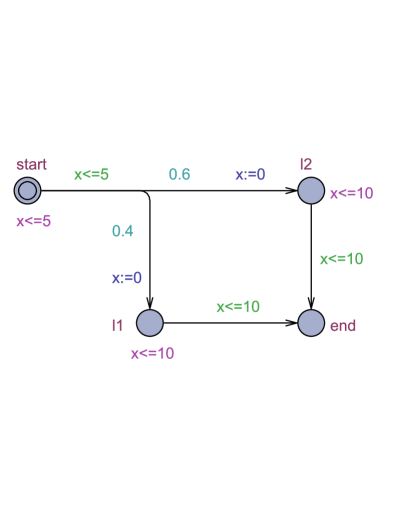
Figure 1: $\mathcal{P}_{1}$: A PTA with two subruns

Example 1.

To demonstrate how one can compute WCET of PTAs, let us consider the PTA given in Fig. 1. Note that the given PTA consists of a single run which can be split into two subruns $r_{1}$ and $r_{2}$, where $r_{1}$ visits locations start, l1 and end while subrun $r_{2}$ visits locations start, l2 and end. The location end represents the halting location of the automaton. Let us denote the edge from start to l1 by $e_{0}$ and the edge from start to l2 by $e_{1}$. Then $weight(e_{0})=0.4$ and $weight(e_{1})=0.6$, while the other edges have probability weight of one. The WCET of this automaton can be obtained by taking the sum of the delays of the two subruns, while maximizing the time delay the automaton can spend at each visited location. That is, $Maxdelay(r_{1})=5*0.4+0.4*10=6$ and $Maxdelay(r_{2})=5*0.6+0.6*10=9$. Hence, $\mathbb{WCET}(\mathcal{P}_{1})=Maxdelay(r_{1})+Maxdelay(r_{2})=15$.

Our goal here is to develop an efficient solution for WCET of cyclic PTAs by accelerating the execution of cycles that can be taken with high probability. Such classes of cycles can degrade the performance of model checking algorithms, since the probability to repeat the cycle converges to zero arbitrarily slowly.

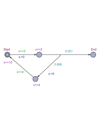
Figure 2: $\mathcal{P}_{2}$: A cyclic PTA which can be taken with high probability

Example 2.

The automaton in Fig. 2 contains a cycle that can be repeated with very high probability, where the likelihood to repeat the cycle gradually decreases. The first time we reach the choice point in Fig. 2, the probability of cycling is $0.999$ while the probability of moving to the ‘End’ state is $0.001$. If we take the cycle then the next time we reach the choice point we will effectively have a lower probability of again taking the cycle ‘choice’. Effectively, the probability here is $0.999\times 0.999$. And so on. In this way, the likelihood of staying within the cycle monotonically decreases and eventually reaches zero (or close enough to be considered as zero).

2.3 The Zone Abstraction and Difference Bound Matrices

The state space of dense-time models can, in general, be infinite (uncountable) and therefore can not be directly model checked. However, researchers in real-time model checking devised an efficient representation of the state space of a TA based on zone-graphs [8, 12]. In a zone graph, zones denote symbolic states. In practice, this provides a more compact representation of the state-space of a given TA model.

A zone is a pair $(l,\varphi)$, where $l$ is a location of a PTA $\mathcal{P}$ and $\varphi$ is a clock zone. The clock zone $succ(\varphi,e)$ will denote the set of clock valuations $v^{{}^{\prime}}$ such that for some $v\in\varphi$ the state $(l^{{}^{\prime}},v^{{}^{\prime}})$ can be reached from the state $(l,v)$ by letting time elapse and by executing the transition $e$. The pair $(l^{{}^{\prime}},succ(\varphi,e))$ will represent the set of successors of $(l,\varphi)$ under the transition $e$. Note that the assignment of the values of the clocks in the initial location of $\mathcal{P}$ is easily expressed as a clock zone since $v(x)=0$ for every clock $x\in X$. Note also that every constraint used in the invariant of an automaton location or in the guard of a transition is a clock zone. Therefore, clock zones can be used for various state reachability analysis algorithms for (probabilistic) timed automata.

Difference bound matrices (DBMs) [7] are the data structures most commonly used for representing the state spaces of (probabilistic) timed automata. A DBM is a two-dimensional matrix that records the difference between upper bounds of clock pairs up to a certain constant. Recall that a clock constraint over the set of clocks $X$ is a conjunction of atomic constraints of the form $x\sim m$ and $x-y\sim n$ where $x,y\in X$, $\sim\in\{\leq,<,=,\geq,>\}$, and $m,n$ are integers. In order to provide a unified form for clock constraints in a DBM we introduce a reference clock $x_{0}\in X$ with the constant value 0 that is not used in any guards or invariants. The matrix is indexed by the clocks in $X$ together with the special clock $x_{0}$. The element $D_{i,j}$ in matrix $D$ is of the form $(n,\prec)$ where $x_{i},x_{j}\in X$, $n$ represents the difference between them, and $\prec\in\{\leq,<\}$. Each row in the matrix represents the bound difference between the value of the clock $x_{i}$ and all the other clocks in the zone, thus a zone can be represented by at most $|X|^{2}$ atomic constraints. This implies that each pair of variables $(x_{i},x_{j})$ ($i\neq j$) will be represented by two atomic constraints $(d_{i,j},\prec)$ and $(d_{j,i},\prec)$.

3 Accelerating Execution of Probabilistic Timed Cycles

In this section we discuss some acceleration techniques that can be used to improve the execution of cycles that may be repeated a high number of times. Let us denote the series of maximal expected delays that results from successive executions of a cycle $\pi$ in a PTA $\mathcal{P}$ by $\mathcal{S}_{\pi}$ and $n$ be a cycle counter. We then use the notations $\mathcal{S}_{\pi}\xrightarrow{p}0$ to denote that the probability of taking the cycle moves to zero, and $\mathcal{S}_{\pi}\xrightarrow{a.s}\zeta$, where $\zeta<\infty$, to denote that the series converges almost surely. However, for any reachable cycle $\pi$ in the PTAs we consider, the series $\mathcal{S}_{\pi}$ converges to zero probability (i.e. the cycle will not be taken forever) and converges with probability one, as discussed in Theorem 3.1. (Note that, as the effective probability of remaining in a cycle reduces every time we take the cycle, we often view the probability at the branch point as reducing in this way.)

Theorem 3.1

Let $\pi$ be a cycle in a PTA model that satisfies Assumption 1. Then (1) $\mathcal{S}_{\pi}\xrightarrow{p}0$ as $n\rightarrow\infty$ and (2) $\mathcal{S}_{\pi}\xrightarrow{a.s}\zeta$ as $n\rightarrow\infty$, where $\zeta<\infty$.

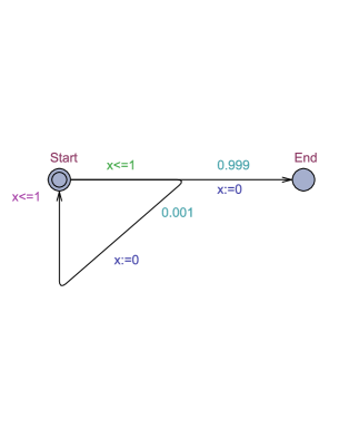
Figure 3: $\mathcal{S}_{\pi}$ converges sufficiently fast

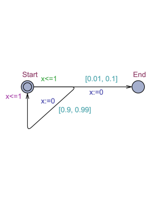
Figure 4: $\mathcal{S}_{\pi}$ converges arbitrary slow

Note that the series $\mathcal{S}_{\pi}$ may converge to zero probability sufficiently fast or arbitrary slow depending on the probability weights of the edges of the cycle. Suppose that we use an approximation bound $\Delta=10^{-6}$ to represent “close enough to zero” in probability when executing cycles in PTAs. So that once the probability that results from successive executions of a cycle becomes smaller than the bound $\Delta$, the cycle will no longer be repeated. It is easy to see then that the cycle in Fig. 4 will be repeated only four iterations (as it becomes “close enough to zero” quite quickly) where the series $\mathcal{S}_{\pi}=(10^{-2}+10^{-4}+10^{-6}+10^{-8})$, while the cycle in Fig. 4 will be repeated around $13808$ iterations where the series $\mathcal{S}_{\pi}=(0.999+0.998001+0.997002+0.996005+...+9\times 10^{-8})$. We now discuss two forms of cycles that may be encountered when analyzing a cyclic PTA model: cycles with constant delays and cycles with periodic delays.

Definition 7

(Cycles with constant delays). Let $\pi$ be a cycle in a PTA model $\mathcal{P}$ and $\verb+delay+(\pi,i)$ be a function that computes the summation of delays of $\pi$ at some arbitrary iteration $i\geq 1$. We say that $\pi$ is a cycle with constant delays if for any two distinct iterations $i,j$ we have $\verb+delay+(\pi,i)=\verb+delay+(\pi,j)$.

Definition 8

(Cycles with periodic delays). Let $\pi$ be a cycle in a PTA model $\mathcal{P}$. We say that $\pi$ is a cycle with periodic delays if the delays of $\pi$ are repeated every $k$ iterations, where $k>1$. That is, $\verb+delay+(\pi,i)=\verb+delay+(\pi,i+k)$.

We now describe the basic formal steps that can be followed to accelerate the execution of a cycle $\pi$ in a PTA model $\mathcal{P}$.

1. Synthesize a delay formula, $\phi_{\pi}$, for the detected cycle $\pi$ that can be used to compute the cumulative delay introduced by successive executions of $\pi$. A delay formula for $\pi$ can be synthesized once a fixed-point of $\pi$ is reached.

2. Find the value of the loop counter $n$ at which the probability to repeat the cycle converges to zero. Recall that for PTAs we consider the probability to repeat cycles decreases monotonically as the iteration number increases.

3. Compute the total expected delay of the cycle $\pi$ using $\phi_{\pi}$.

4. Compute the clock zone that results from collapsing the cycle’s iterations.

5. Update the probability weights of the automaton edges that have been affected by the acceleration process.

6. Restart the corresponding constructed Markov chain of $\mathcal{P}$.

We first discuss how one can synthesize a formula for computing expected delay of cycles with constant delays and cycles with periodic delays.

Definition 9

(Synthesizing formulae for cycles with constant delays). Let $\mathcal{P}=(L,\ell_{0},L_{f},\mathcal{X},Act,inv,E,\mathcal{L})$ be a PTA and $(e_{0},...,e_{m-1})\in E_{\pi}$ be the sequence of edges of a reachable cycle $\pi$ in $\mathcal{P}$ whose delay intervals between iterations are constant. Let $T_{0}^{\max},...,T_{m-1}^{\max}$ be the maximum delay bounds that can elapse at the cycle’s locations $src(e_{0}),...,src(e_{m-1})$. The cumulative delays that result from successive executions of $\pi$ can be computed as follows

$$\phi_{\pi}^{c}=\sum_{a=0}^{n}\sum_{b=0}^{m-1}\mathcal{I}*(\prod_{c=0}^{m-1}weight(e_{c}))^{a}*(\prod_{d=0}^{b-1}weight(e_{d}))*T_{b}^{\max}$$

where $\mathcal{I}$ represents the initial probability value at which the cycle $\pi$ has been reached during the analysis. The first summation operator in the formula is used to iterate through the cycle until the probability to repeat the cycle effectively converges to zero, while the second summation operator is used to iterate through the control locations of the cycle at each iteration. Since the control locations of the cycle can be reached with different probability values at each different iteration, the expected delays that result from visiting these locations can vary between iterations. However, the formula in Definition 9 can be simplified further as $\sigma=\prod_{c=0}^{m-1}weight(e_{c})$ is constant. This yields the following formula

$$\phi_{\pi}^{c}=\sum_{a=0}^{n}\sum_{b=0}^{m-1}\mathcal{I}*\sigma^{a}*(\prod_{c=0}^{b-1}weight(e_{c}))*T_{b}^{\max}.$$

It remains to discuss how to compute the value of $n$ (i.e. the number of times the cycle can be repeated). To find the value of $n$ we need to solve the simple exponential formula $\sigma^{n}=\dfrac{\Delta}{\mathcal{I}}$. However, by taking the natural logarithmic of both sides, then $n$ can be computed as follows

$$n=(\dfrac{ln(\Delta)}{ln(\sigma*\mathcal{I})}).$$

Definition 10

(Synthesizing formulae for cycles with periodic delays). Let $\mathcal{P}=(L,\ell_{0},L_{f},\mathcal{X},Act,inv,E,\mathcal{L})$ be a PTA and $(e_{0},...,e_{m-1})\in E_{\pi}$ be the sequence of edges of a reachable cycle $\pi$ in $\mathcal{P}$. Suppose that $\pi$ is a cycle with periodic delays so that the delays are repeated every $k$ iterations. The cumulative delays that result from successive executions of $\pi$ can be computed as follows

$$\phi_{\pi}^{p}=\sum_{a=0,a+k}^{n}\sum_{b=1}^{k}\sum_{c=0}^{m-1}\mathcal{I}*(\prod_{d=0}^{m-1}weight(e_{d}))^{a}*(\prod_{e=0}^{b-1}weight(e_{e}))*T_{(b,c)}^{\max}$$

where $k$ represents the rate (i.e. number of iterations) at which delays of $\pi$ are repeated, and $T_{(b,c)}^{\max}$ is the maximum delay that $\mathcal{P}$ can spend at location $src(e_{c})$ at iteration $b$ where $b\in\{1,..k\}$ and $c\in\{0,..,m-1\}$. However, since the cycle contains periodic delays then every $k$ iterations the counter $b$ needs to be reset. Similar to cycles with constant delays, the given formula can be simplified to

$$\phi_{\pi}^{p}=\sum_{a=0,a+k}^{n}\sum_{b=0}^{k-1}\sum_{c=0}^{m-1}\mathcal{I}*\sigma^{a}*(\prod_{d=0}^{b-1}weight(e_{d}))*T_{(b,c)}^{\max}.$$

The next step in the process is to compute the accelerated clock zone that results from collapsing iterations of the cycle. Recall that zones provide a representation of sets of clock interpretations as constraints on (lower and upper) bounds on individual clocks and clock differences. Let $k$ be the iteration number at which the delay of the cycle becomes constant and $n$ be the value of the cycle counter at which the probability to repeat the cycle effectively converges to zero. We can compute the clock zone that results from accelerating such a cycle as follows.

• Updating lower/upper bounds of the automaton clocks. Updating the automaton clocks during acceleration is an easy task as the delays of the cycle are constant between iterations. Hence, the lower and upper bound of a clock $z$ can be updated as follows.

  $$D_{0,z}^{n}=(D_{0,z}^{k}+(n-k)*(D_{0,z}^{k}-D_{0,z}^{k-1}))$$

  $$D^{n}_{z,0}=(D_{z,0}^{k}+(n-k)*(D_{z,0}^{k}-D_{z,0}^{k-1}))$$

• Updating diagonal constraints of the automaton clocks. Updating this set of constraints is also a straightforward task. Let $z_{1}$ and $z_{2}$ be two clocks in the automaton being accelerated. Then the diagonal constraints involving $z_{1}$ and $z_{2}$ can be updated as follows.

  $$D_{z_{1},z_{2}}^{n}=D_{z_{1},z_{2}}^{k}+(D^{k}_{z_{1},0}-D^{k}_{0,z_{2}})*(n-k)$$

  $$D_{z_{2},z_{1}}^{n}=D_{z_{2},z_{1}}^{k}+(D^{k}_{z_{2},0}-D^{k}_{0,z_{1}})*(n-k)$$

We now turn to discuss how to compute the accelerated clock zone that results from collapsing the iterations of cycles with periodic delays. For this class of cycles, the lower and upper bounds of the automaton clocks can be updated as follows, where the variable $k$ used in the formulae to represent the rate (number of iterations) at which delays are repeated.

$$D_{0,z}^{n}=((D_{0,z}^{k}-D_{0,z}^{0})*\lfloor n/k\rfloor)+\sum_{i=1}^{(n\%k)}(D_{0,z}^{i}-D_{0,z}^{i-1})$$

$$D_{z,0}^{n}=((D_{z,0}^{k}-D_{z,0}^{0})*\lfloor n/k\rfloor)+\sum_{i=1}^{(n\%k)}(D_{z,0}^{i}-D_{z,0}^{i-1})$$

The diagonal constraints of the automaton clocks can be updated as follows.

$$D_{z_{1},z_{2}}^{n}=((D_{z_{1},z_{2}}^{k}-D_{z_{1},z_{2}}^{0})*\lfloor n/k\rfloor)+\sum_{i=1}^{(n\%k)}(D_{z_{1},z_{2}}^{i}-D_{z_{1},z_{2}}^{i-1})$$

$$D_{z_{2},z_{1}}^{n}=((D_{z_{2},z_{1}}^{k}-D_{z_{2},z_{1}}^{0})*\lfloor n/k\rfloor)+\sum_{i=1}^{(n\%k)}(D_{z_{2},z_{1}}^{i}-D_{z_{2},z_{1}}^{i-1})$$

The next important step of the acceleration process is to update the probability weights of the edges of the automaton that have been affected by the acceleration. Note that, after acceleration, the probability weights of some edges of the cycle will have decreased (e.g. will be set to zero) and hence the probability weights of some other edges of the automaton need to be updated (increased) in order to maintain the overall probability distribution at states. This step can also be performed according to the update rules given in Definition 11.

Definition 11

(Probability update rules after acceleration). Let $\mathcal{P}=(L,\ell_{0},L_{f},\mathcal{X},Act,inv,E,\mathcal{L})$ be a PTA and $(e_{0},e_{1},...,e_{m-1})\in E_{\pi}$ be the sequence of edges of a reachable cycle $\pi$ in $\mathcal{P}$. Then after accelerating the execution of $\pi$ the probability weights of some edges in $\mathcal{P}$ will be updated as follows

1. Let $E_{out}$ be the set of edges in the set $out(src(e_{i}))\setminus e_{i}$, where $e_{i}\in E_{\pi}$. Then for each edge $e_{j}\in E_{out}$, such that $0<weight(e_{j})<1$, update the probability weight of $e_{j}$ as follows

   $$\overline{weight(e_{j})}=weight(e_{j})+\frac{weight(e_{j})*weight(e_{i})}{\sum_{e_{k}\in E_{out}}weight(e_{k})}$$

   where $weight(e_{j})$ represents the probability weight of the edge $e_{j}$ in the prior distribution (before acceleration) and $\overline{weight(e_{j})}$ represents the probability weight of the edge $e_{j}$ in the new distribution (after acceleration).

2. For each edge $e_{i}\in E_{\pi}$ whose $weight(e_{i})<1$ set $weight(e_{i})$ to zero.

The last step of the process involves restarting the Markov chain of the model $\mathcal{P}$ by setting the initial probability of the system to one. The new initial state of the model will be chosen according to available probabilistic choices.

3.1 Effectiveness of Acceleration

The effectiveness of the proposed acceleration (the possible reduction on the size of the generated zone graph) depends on four factors: (a) the value of $\sigma$ (the rate at which the probability to repeat the cycle is decreasing), (b) the length of the cycle being accelerated, (c) the approximation bound $\Delta$ used to represent “convergence to zero”, and (d) the size of the states of the model (the number of the clocks in the model as this can affect the size of the generated DBMs).

Theorem 3.2

(Effectiveness of acceleration). Let $\mathcal{P}$ be a PTA that satisfies Assumption 1 and $\pi$ be a reachable cycle in $\mathcal{P}$. Then the proposed acceleration can reduce the size of the generated zone graph of $\mathcal{P}$ by $((n-k)\times length(\pi))$ states, where $n$ represents the number of times the cycle can be repeated, $k$ represents the iteration number at which a fixed-point of $\pi$ can be reached, and $length(\pi)$ represents the number of transitions of $\pi$.

Let us denote the zone graph that results from model checking the non-accelerated cyclic PTA automaton $\mathcal{P}$ in which all system states are explored by $\mathcal{Z}(\mathcal{P})$, and the graph that results from model checking the accelerated version of $\mathcal{P}$ where cycles iterations are collapsed by $\mathcal{Z}(\mathcal{P^{\mathfrak{a}}})$. Suppose that branches or subruns of $\mathcal{P}$ contain $m$-cycles $\{\pi_{1},...,\pi_{m}\}$. Then the reduction gained ($RG$) from accelerating the executions of cycles in $\mathcal{P}$ can be measured as follows

$$RG=(|\mathcal{Z}(\mathcal{P})|-|\mathcal{Z}(\mathcal{P^{\mathfrak{a}}}|)=\sum_{i=1}^{m}((n_{i}-k_{i})\times length(\pi_{i})).$$

The reader can easily construct an example where the series $\mathcal{S}_{\pi}$ (the series that results from successive executions of $\pi$) converges almost surely while the series converges to zero probability arbitrarily slowly.

4 A Zone-based Algorithm for WCET of Cyclic PTAs

In this section, we describe a zone-based algorithm that can be used to compute the expected WCET of cyclic PTAs. Each node in the computed zone graph of the given PTA model has the form $(\ell,Z,\alpha,sts,cnt)$ where the variable $sts$ (which is assigned to each state) is used to detect whether there exists a cycle on locations in the behavior of the automaton. The variable $sts$ can take values from the set $\{0,1,2\}$. When it is 0 it means that the location has not been visited before, when it is 1 it means the location has been visited before but not fully explored, and when it is 2 it means that everything reachable from that location has been explored. We assume that the reader is familiar with the classical DFS algorithm with the labeling process of nodes to unvisited (0), being explored (1), and finished (2) and hence we omit these details. The variable $\alpha$ maintains the probability value at which the state has been reached. The variable $cnt$ is used to keep track of the iteration number of a detected cycle, where $cnt$ is incremented every time a full iteration of the cycle is completed and reset once the cycle is skipped. By examining the value of the variable $cnt$ when a fixed-point of a cycle is reached, we can then distinguish between different forms of cycles.

Definition 12

(Detecting cycles with constant/periodic delays.) Let $\pi$ be a reachable cycle in a PTA model $\mathcal{P}$. Suppose that during the analysis of $\pi$ the two states $s$ and $s^{\prime}$ have been reached where $(s.\ell=s^{\prime}.\ell\land(s.Z\setminus inact=s^{\prime}.Z\setminus inact))$ (i.e. a fixed-point has been reached w.r.t. the active clocks of the cycle). Suppose further that $s.cnt<s^{\prime}.cnt$ so that the state $s^{\prime}$ has been reached in an iteration that is greater than state $s$. We can then determine the class of the cycle $\pi$ by examining the characteristics of the reached fixed-point as follows

1. We say that $\pi$ is a cycle with constant delays or a cycle whose delays become constant after some iterations if the following condition holds

   $$(s.\ell=s^{\prime}.\ell\land(s.Z\setminus inact=s^{\prime}.Z\setminus inact)\land(s^{\prime}.cnt\leq 3\lor(s^{\prime}.cnt-s.cnt)=1))$$

2. We say that $\pi$ is a cycle with periodic delays if the following condition holds

   $$(s.\ell=s^{\prime}.\ell\land(s.Z\setminus inact=s^{\prime}.Z\setminus inact)\land s^{\prime}.cnt>3\land(s^{\prime}.cnt-s.cnt)>1)$$

It is interesting to note that the set of clock zones that result from the first iteration of a cycle can be arbitrary zones as the initial zone at which the cycle is reached has not been obtained from the cycle’s internal computations. Hence, if a fixed-point of a cycle is reached within the first three iterations, or within any two consecutive iterations of the cycle, then we know that the cycle must have constant delays. Otherwise, the cycle will have periodic delays. Note that the tests described in Definition 12 can detect all forms of cycles with constant or periodic delays, regardless of their underlying syntactic structures.

l‌​

1:Input: $(\mathcal{P}$)

2:Output: $\textbf{double}~{}\verb+WCET+:=0$

3:double $\alpha:=1,prob:=1,\Delta:=10^{-6}$

4:int $sts:=0,cnt:=0$

5:clock $\verb+CLK+$

6:WAIT := $\{(l_{0},Z_{0},\alpha,sts,cnt)\}$, PASSED := $\emptyset$

7:while WAIT $\neq~{}\emptyset$ do

8:     select $s$ from WAIT

9:     add $s$ to PASSED

10:     for each $e\in out(s.\ell)$ do

11:         $prob:=(s.\alpha*weight(e))$

12:         $s^{\prime}:=succ(s.Z,e)$

13:         if $s^{\prime}.\ell=s^{{}^{\prime\prime}}.\ell\land s^{{}^{\prime\prime}}.sts=1\land s^{\prime}.Z=s^{{}^{\prime\prime}}.Z$ for any $s^{{}^{\prime\prime}}\in$ PASSED then

14:              $L_{\pi}$ := $ComputeLocationsofCycle()$

15:              $\phi_{\pi}:=SynthDelayFormula(L_{\pi})$

16:              if $s^{\prime}.cnt\leq 3~{}\lor((s^{\prime}.cnt-s^{{}^{\prime\prime}}.cnt)=1)$ then

17:                  for each $\ell\in L_{\pi}$ such that $out(\ell)>1\ \textbf{do}$

18:                       add $(\ell,AccelConstCycle(L_{\pi}))$ to WAIT

19:                  end for

20:              else if $s^{\prime}.cnt>3~{}\land((s^{\prime}.cnt-s^{{}^{\prime\prime}}.cnt)>1)$ then

21:                  for each $\ell\in L_{\pi}$ such that $out(\ell)>1\ \textbf{do}$

22:                       add $(\ell,AccelPeriodCycle(L_{\pi}))$ to WAIT

23:                  end for

24:              end if

25:              $s^{\prime}.cnt:=0$

26:         else if $s^{\prime}.\ell=s^{{}^{\prime\prime}}.\ell\land s^{{}^{\prime\prime}}.sts=1\land s^{\prime}.\dot{Z}\neq s^{{}^{\prime\prime}}.\dot{Z}\land prob>\Delta$
          for any $s^{{}^{\prime\prime}}\in$ PASSED then

27:              $\verb+WCET+:=\verb+WCET++prob*(|s^{\prime}.Z_{(CLK,0)}-s.Z_{(CLK,0)}|)$

28:              $s^{\prime}.cnt++$

29:              add $s^{\prime}$ to WAIT

30:         else if $s^{\prime}.\ell=s^{{}^{\prime\prime}}.\ell\land s^{{}^{\prime\prime}}.sts=1\land s^{\prime}.\dot{Z}\neq s^{{}^{\prime\prime}}.\dot{Z}\land prob<\Delta$
          for any $s^{{}^{\prime\prime}}\in$ PASSED then

31:              $s^{\prime}.cnt:=0$

32:              $prob:=1$

33:         else

34:              $\verb+WCET+:=\verb+WCET++prob*(|s^{\prime}.Z_{(CLK,0)}-s.Z_{(CLK,0)}|)$

35:              add $s^{\prime}$ to WAIT

36:         end if

37:     end for

38:end while

39:return WCET

Algorithm 1 An algorithm for computing WCET of deterministic PTAs

Algorithm 1 uses an extra clock CLK to keep track of time delays that can elapse at each state of the model. The algorithm uses a number of operations to handle cycles in the input PTA. The operation $ComputeLocationsofCycle()$ is used to compute the set of control locations of the detected cycle in the form $(\ell_{0},...,\ell_{m-1})$. This is necessary in order to compute the set of final states when accelerating the execution of the cycle. The operation $SynthDelayFormula()$ is used to synthesize a delay formula for the detected cycle once a fixed point is reached. Two acceleration procedures are used, namely $AccelConstCycle()$ which is used to accelerate cycles with constant delays, and $AccelPeriodCycle()$ which is used to accelerate cycles with periodic delays. Each of these acceleration procedures consists of a number of operations as described in Section 3. Note that in some cases, however, Algorithm 1 may compute more than one final state when accelerating the execution of a detected cycle $\pi$, depending mainly on the structure of the cycle. That is, for each outgoing edge $e_{j}$ of the cycle’s location $\ell$, where $e_{j}\not\in E_{\pi}$, the algorithm computes a final state. So that if there are $k$ control locations of the cycle $\pi$ that have more than one outgoing edge then the algorithm computes $k$ final states.

It is interesting to note also that the algorithm uses the activity abstraction when searching for a fixed-point of visited cycles. The activity abstraction ignores clocks that are inactive at some point during the exploration. A clock is active within a cycle $\pi$ if its value at some location of the cycle may influence the future evolution of the cycle. This can happen either when the clock appears in the invariant condition of some location of the cycle, it is tested in the condition of some of the edges of the cycle, or an active clock takes its value when moving through an edge of the cycle. We write $s.\dot{Z}$ to refer to the set of clock constraints involving active clocks at state $s$.

Theorem 4.1

Algorithm 1 computes a sound estimation of WCET of PTAs.

To compute the WCET of a cyclic PTA, Algorithm 1 requires that each reachable cycle is repeated until the probability that results from successive executions of the cycle converges to zero. Since there is actually no end (it is not possible, theoretically, to reach zero), Algorithm 1 uses an arbitrary stopping point $\Delta$, which is chosen in a way such that any errors accumulated across several cycles are minimized and so that zero can be effectively reached. This ensures the sound estimation of whole automaton WCET.

5 Implementation

In this section we briefly summarise our prototype implementation of the model checking algorithms given in Section 4. It is important to note that the goal of our implementation is to validate the presented algorithms, rather than to devise an efficient implementation; this will be the subject of our future work.

The prototype implementation has been developed using the opaal tool [6] which has been designed to rapidly prototype new model checking algorithms. The opaal tool is implemented in Python and is a standalone model checking engine. We use the open source UPPAAL DBM library for the internal symbolic representation of time zones in the algorithms.

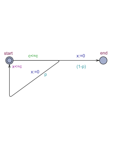
Figure 5: Demonstrating example

We consider here one example of cyclic PTA (see Fig. 5), but we verify it under four different settings: (a) when $p=0.001$ and $c=1$, (b) when $p=0.001$ and $c=10^{6}$, (c) when $p=0.999$ and $c=1$, and (d) when $p=0.999$ and $c=10^{6}$. It is easy to see that the WCET of the automaton under these four settings will be different, as the number of times the cycle will be repeated and the time that can elapse at each iteration will be different. For this example, we set $\Delta=10^{-6}$. It is easy to see that the cycle in the given automaton has constant delays as the active clock of the cycle (clock x) is reset each time the cycle is executed and hence after two iterations the search will reach a fixed-point at location Start. The synthesized delay formula for computing WCET of the cycle will be $\phi_{\pi}=\sum_{i=1}^{n}(p^{i}*c)$, where $n=\dfrac{ln(\Delta)}{ln(p)}$. The WCET as computed by the algorithm for the four cases is as follows: (a) WCET = 1.001, (b) WCET = 1001001.001, (c) WCET = 1000, and (d) WCET = $10^{9}$. For cases (a) and (b) the cycle needs to be repeated only two times, while for cases (c) and (d) the cycle needs to be repeated about 13808 times. However, the algorithm collapsed the iterations of the cycle and hence it avoided the explicit repeated exploration of the cycle. The algorithm returned an answer for each case almost instantly. Note that there is no available implementation for the algorithms presented in [10, 9], and hence we were not able to report any result about their performance in presence of cycles. However, the algorithms in [10, 9] are not optimized to check WCET of PTAs (specially those which contain cycles that can be repeated very often due to high probabilities.)

Nested Cycles and Intersecting cycles

Algorithm 1 can handle only cyclic PTAs that satisfies the flatness assumption, wherein each location can be part of at most one cycle. Hence, nested cycles and intersecting cycles (i.e. two or more cycles which have at least one control location in common) cannot be handled using Algorithm 1. The presence of such classes of cycles complicates the formal verification of expected WCET of PTAs. In particular, if there is a nested cycle in the automaton, then if some inner cycle is detected and then collapsed, the adjustment of the weights performed (as detailed in section 3) (along with the addition of the visited states to the PASSED list in the algorithm) would impact the ability to accurately collapse an “outer cycle” with arcs composed in part of the inner cycle. Furthermore, the order at which intersecting cycles are executed can affect the outcome of the WCET analysis, depending on the way the probabilistic choices at common control location are resolved. In future work, we aim to extend the algorithm to handle complex forms of cycles including nested cycles and intersecting cycles.

6 Conclusion and Future Work

We have described a model checking algorithm which can be applied to verify expected WCET of probabilistic timed systems with cyclic behavior. Indeed, the presence of cycles that can be repeated a very high number of times in the input timed probabilistic model can degrade the performance of the model checking algorithm. However, we have shown that it is possible to accelerate the execution of probabilistic timed cycles without adversely affecting the outcome of the analysis. In a future work, we aim to reconsider the problem while allowing non-deterministic choices between edges, where the precise complexity of the expected WCET problem for cyclic PTAs with non-determinism is still open.

References

- [1] Omar Al-Bataineh, Mark Reynolds, and Tim French. Accelerating worst case execution time analysis of timed automata models with cyclic behaviour. Formal Aspect of Computing, 27(5-6):917–949, 2015.
- [2] Omar Al-Bataineh, Mark Reynolds, and Tim French. Finding minimum and maximum termination time of timed automata models with cyclic behaviour. Theoretical Computer Science, 665:87 - 104, 2017.
- [3] Rajeev Alur, Costas Courcoubetis, and David Dill. Model-checking for probabilistic real-time systems (extended abstract). In Proceedings of the 18th International Colloquium on Automata, Languages and Programming, pages 115–126. Springer-Verlag New York, Inc., 1991.
- [4] Rajeev Alur and David L. Dill. A theory of timed automata. Theoretical Computer Science, 126(2):183–235, 1994.
- [5] Danièle Beauquier. On probabilistic timed automata. Theoretical Computer Science, 292(1):65–84, January 2003.
- [6] Andreas Engelbredt Dalsgaard, René Rydhof Hansen, Kenneth Yrke Jørgensen, Kim Guldstrand Larsen, Mads Chr. Olesen, Petur Olsen, and Jirí Srba. opaal: A lattice model checker. In NASA Formal Methods’11, pages 487–493, 2011.
- [7] David Dill. Timing assumptions and verification of finite-state concurrent systems. In Proceedings of the international workshop on Automatic verification methods for finite state systems, pages 197–212. Springer-Verlag New York, Inc., 1990.
- [8] Thomas A. Henzinger, Xavier Nicollin, Joseph Sifakis, and Sergio Yovine. Symbolic model checking for real-time systems. Information and Computation, 111:394–406, 1992.
- [9] Aleksandra Jovanovi, Marta Kwiatkowska, Gethin Norman, and Quentin Peyras. Symbolic optimal expected time reachability computation and controller synthesis for probabilistic timed automata. Theoretical Computer Science, 669:1–21, 2017.
- [10] Marta Kwiatkowska, G. Norman, D. Parker, and J. Sproston. Performance analysis of probabilistic timed automata using digital clocks. In Proceeding of Formal Modeling and Analysis of Timed Systems (FORMATS’03), volume 2791 of LNCS, pages 105–120. Springer-Verlag, 2003.
- [11] Marta Z. Kwiatkowska, Gethin Norman, Roberto Segala, and Jeremy Sproston. Automatic verification of real-time systems with discrete probability distributions. Theoretical Computer Science, 282:101–150, 2002.
- [12] Mihalis Yannakakis and David Lee. An efficient algorithm for minimizing real-time transition systems. Formal Methods of System Design, 11(2):113–136, 1997.