The Ehrenfest Urn Model with Interaction

Abstract

We studied the Ehrenfest urn model in which particles in the same urn interact with each other. Depending on the nature of interaction, the system undergoes a first-order or second-order phase transition. The relaxation time to the equilibrium state, the Poincare cycles of the equilibrium state and the most far-from-equilibrium state, and the duration time of the states during first-order phase transition are calculated. It was shown that the scaling behavior of the Poincare cycles could be served as an indication to the nature of phase transition, and the ratio of duration time of the states could be a strong evidence of the metastability during first-order phase transition.

I I. Introduction

Historically, the Boltzmann’s $H$ theorem based on the assumption of molecular chaos singles out a direction of time, which led to two pardoxes huang . The first one, so-called reversal paradox, states that the $H$ theorem is inconsistent with the time reversal invariance. The Poincare theorem poincare requires that the system should return to its initial state (up to an arbitrarily small neighborhood) after sufficiently long time. This fact implies reversibility of the dynamical system, leading to the so-called recurrence paradox. Later on, the Ehrenfest urn model ehrenfest was proposed to resolve the paradoxes and clarify the relationship between reversible dynamics and irreversible thermodynamics.

The Ehrenfest model deals with two urns with total $N$ particles. Each particle is randomly chosen with equal probability in such a way that it is taken from one urn to another urn. It is found that the relaxation time for the system to reach its equilibrium is proportional to $N$, and the Poincare cycle of the most far-from-equilibrium state is proportional to $2^{N}$ kac .

Since then, the Ehrenfest model was generalized such that the jumping rates between two urns are unbalanced siegert ; klein , the system of two urns becomes multiurn kao03 ; kao04 ; nagler05 , and multiurn are connected in a complex network clark . Fluctuation distribution of the model was also studied hauert ; bakar09 ; bakar10 .

The Ehrenfest model was also applied to understand the granular system by inducing different effective temperatures with respect to gravitational field in different urns, which turns out to exhibit the spatial separation (symmetry-breaking) phase transition lipowski02a ; lipowski02b ; coppex . This model was also solved analytically shim .

By considering the continuum limit of time step in the evolution of the probability of the state, the linear Fokker-Planck equation is obtained kac ; nagler99 . Modification of the Ehrenfest model by incorporating nonlinear contribution to the Fokker-Planck equation recently calls for attention curado ; nobre ; casas , which is motivated by the processes associated with anomalous-diffusion phenomena bouchaud ; boon ; lutsko . The generalized $H$ theorem for the nonlinear Fokker-Planck equation was studied by many authors in recent years schwammle ; shiino ; frank ; chavanis .

Although many attempts were made to modify the Ehrenfest model, none of them has been associated with explicit particle interaction, to our knowledge. The model that we modified exhibits the (first-order and second-order) phase transition depending on the nature of interaction. We also calculate the relaxation time to the equilibrium state, the Poincare cycles of both the equilibrium and the most far-from-equilibrium states, and the duration time of the states during the first-order phase transition. Finally, we point out that the scaling behavior of the Poincare cycle could be served as an indication of the nature of the phase transition, and the ratio of duration time of the states could be a strong evidence of the metastability during first-order phase transition.

II II. Ehrenfest model with interaction

We present our model as follows. There are $N$ particles distributed into two urns. The number of particle in the left and right urns are $n$ and $N-n$, respectively. Since the total particle number $N$ is fixed, we label the state of the system by its particle number in the left urn, denoted by $|n\rangle$.

Unlike the original Ehrenfest model, we introduce particle interaction in the same urn. Two particles of different urns do not interact. The total energy $E=\frac{J}{2}(n(n-1)+(N-n)(N-n-1))$ with energy coupling $J$. The interaction is attractive (replusive) if $J$ is negative (positive). When a particle jumps from the left to the right urn, $\Delta E=-J(2n-N-1)$. To satisfy the principle of detailed balance, we should have the restriction on the transition probability such that

$$\frac{T_{n,n-1}}{T_{n-1,n}}={\rm e}^{\beta\Delta E}={\rm e}^{-\frac{g}{N}(2n-N-1)}$$ (1)

where $T_{n\pm 1,n}$ is the transition probability from the state $|n\rangle$ to $|n\pm 1\rangle$, $\beta$ is the inverse of effective temperature, and we introduce the coupling constant $g\equiv NJ\beta$ such that $\Delta E$ is extensive (proportional to $N$ given fixed $g$). There is a degree of freedom to choose the transition probability; however, we adopt

$$T_{n-1,n} = \frac{1}{{\rm e}^{-\frac{g}{N}(2n-N-1)}+1}$$ (2)

$$T_{n,n-1} = \frac{1}{{\rm e}^{\frac{g}{N}(2n-N-1)}+1}$$ (3)

Note that $T_{n-1,n}=T_{n,n-1}=\frac{1}{2}$ if the interaction is turned off. Different proportionality implies different time scale chosen. Besides the particle interaction, we further introduce the jumping rate from one urn to another urn, which is independent of the particle interaction. Suppose the probability of jumping rate from the left (right) to the right (left) urn is $p(q)$. For convenience, we restrict $p+q=1$. Again this restriction only changes the time scale.

After $s$ steps from the initial state $|n_{0}\rangle$, the probability of the state $|n\rangle$ is denoted by $\langle n|p(s)|n_{0}\rangle$, where $p(s)$ is the corresponding operator. As illustrated in Fig. 1, one have the recurrence relation from the $(s-1)$-th to $s$-th step such that

$$\langle n|p(s)|n_{0}\rangle=W_{n,n-1}\langle n-1|p(s-1)|n_{0}\rangle+W_{n,n+1}\langle n+1|p(s-1)|n_{0}\rangle+W_{n,n}\langle n|p(s-1)|n_{0}\rangle$$ (4)

where $W_{n-1,n}=\frac{n}{N}pT_{n-1,n}$, $W_{n,n-1}=\frac{N-n+1}{N}qT_{n,n-1}$, and $W_{n,n}=1-W_{n-1,n}-W_{n+1,n}$.

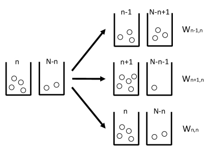
Figure 1: Schematic Diagram to illustrate the transition in our model.

It is convenient to rewrite the recurrence relation in a matrix form. Let the state vector

$$\psi(s)=\left(\begin{array}[]{c}\langle 0|p(s)|n_{0}\rangle\\ \langle 1|p(s)|n_{0}\rangle\\ \vdots\\ \langle N|p(s)|n_{0}\rangle\\ \end{array}\right)$$ (9)

The normalization condition (probability conservation) of the state vector is $\sum_{n=0}^{N}\psi_{n}(s)=\sum_{n=0}^{N}\langle n|p(s)|n_{0}\rangle=1$ for any $s$. Define the matrix $M_{nm}=\langle n|p(1)|m\rangle$ so that $\psi(s)=M\psi(s-1)$. In general, $\psi(s)=M^{s}\psi(0)$. Based on the normalization condition of the state vectors, the matrix $M$ should satisfy

$$\sum_{n=0}^{N}(M^{s})_{nm}=1$$ (10)

for $m=0,1,\ldots,N$ and $s\geq 1$. $M^{s}$ can be evaluated if the eigenvalues $\lambda_{m}$ and eigenvectors $\phi(m)=(\phi_{0}(m),\phi_{1}(m),\ldots,\phi_{N}(m))^{t}$ of $M$ are known, and so

$$M^{s}=A\Lambda^{s}A^{-1}$$ (11)

where $A$ and $\Lambda$ are matrices of dimension $(N+1)\times(N+1)$. Their components are $A_{nm}=\phi_{n}(m)$ and $\Lambda_{nm}=\lambda_{m}\delta_{nm}$.

The eigensystem becomes

$$\frac{N-n+1}{N}\frac{q}{{\rm e}^{\frac{g}{N}(2n-N-1)}+1}\phi_{n-1}+\frac{n+1}{N}\frac{p}{{\rm e}^{-\frac{g}{N}(2n-N+1)}+1}\phi_{n+1}$$

$$+\left(1-\frac{n}{N}\frac{p}{{\rm e}^{-\frac{g}{N}(2n-N-1)}+1}-\frac{N-n}{N}\frac{q}{{\rm e}^{\frac{g}{N}(2n-N+1)}+1}\right)\phi_{n}=\lambda\phi_{n}$$ (12)

The indices $m$ to $\lambda$ and $\phi_{n}$ is omitted without causing any confusion. We found no exact solution to the eigenproblem except for some special cases, e.g. the cases in which $g=0$ and $g\rightarrow-\infty$ (See Appendix A and B for details). If $\lambda_{N}=1$ (we label its index $N$),

$$\phi_{n}(N)=\frac{N!}{n!(N-n)!}p^{N-n}q^{n}{\rm e}^{\frac{g}{N}n(N-n)}$$ (13)

in which the eigenstate could be verified by directly substitution into Eq. (II).

III III. Mean Particle Number

The mean particle number after $s$ steps,

$$\langle n\rangle_{s} = \sum_{n=0}^{N}n\psi_{n}(s)$$ (14)

$$= \sum_{n=0}^{N}n(M^{s}\psi(0))_{n}$$

$$= \sum_{n=0}^{N}\sum_{m,k=0}^{N}nA_{nm}\lambda_{m}^{s}A_{mk}^{-1}\psi_{k}(0)$$

Suppose there is an unique state of unity eigenvalue, says, $\lambda_{N}=1$, and all the remaining eigenvalues are less than unity, as $s\rightarrow\infty$, the mean value $\langle n\rangle$ is defined as

$$\langle n\rangle\equiv\langle n\rangle_{\infty}=\sum_{n=0}^{N}\sum_{k=0}^{N}nA_{nN}A_{Nk}^{-1}\psi_{k}(0)$$ (15)

By taking the limit $s\rightarrow\infty$ in Eq. (10), we get $\sum_{n=0}^{N}A_{nN}A_{Nm}^{-1}=1$ for any $m$. Hence

$$A_{Nm}^{-1}=\frac{1}{\sum_{n=0}^{N}A_{nN}}=\frac{1}{\sum_{n=0}^{N}\phi_{n}(N)}$$ (16)

which is independent of $m$. Substitute Eq. (16) into Eq. (15),

$$\langle n\rangle = \sum_{n=0}^{N}n\phi_{n}(N)\frac{1}{\sum_{n=0}^{N}\phi_{n}(N)}\sum_{k=0}^{N}\psi_{k}(0)$$ (17)

$$= \frac{\sum_{n=0}^{N}n\phi_{n}(N)}{\sum_{n=0}^{N}\phi_{n}(N)}$$

In general, there is no closed form for Eq. (17) if $N$ is finite. If $N$ is large enough, we could derive the asymptotic result. Notice that, by using the Stirling formula mathews , one can rewrite Eq. (13) as $\phi_{n}(N)=\exp(Nf(\frac{n}{N})-\frac{1}{2}\log(2\pi\frac{n}{N}(1-\frac{n}{N})N)+O(N^{-1}))$. Then the denominator in Eq. (17)

$$\sum_{n=0}^{N}\phi_{n}(N)=\left(\frac{N}{2\pi}\right)^{\frac{1}{2}}\int_{0}^{1}dx\frac{{\rm e}^{Nf(x)}}{\sqrt{x(1-x)}}$$ (18)

where $x=\frac{n}{N}$, the proportion of particle number in the left urn, and

$$f(x) = -x\ln x-(1-x)\ln(1-x)$$ (19)

$$+(1-x)\ln p+x\ln q+gx(1-x)$$

As $N$ is large enough, the integral is asymptotically

$$\left(\frac{N}{2\pi}\right)^{\frac{1}{2}}\sum_{\{x_{\rm sp}\}}\frac{{\rm e}^{Nf(x_{\rm sp})}}{\sqrt{x_{\rm sp}(1-x_{\rm sp})}}\int_{0}^{1}dx{\rm e}^{\frac{N}{2}f^{\prime\prime}(x_{\rm sp})(x-x_{\rm sp})^{2}}$$ (20)

$$= \sum_{\{x_{\rm sp}\}}\frac{{\rm e}^{Nf(x_{\rm sp})}}{\sqrt{x_{\rm sp}(1-x_{\rm sp})}|f^{\prime\prime}(x_{\rm sp})|^{\frac{1}{2}}}$$

where $\{x_{\rm sp}\}$ is the set of the saddle points satisfying $f^{\prime}(x_{\rm sp})=0$ and $f^{\prime\prime}(x_{\rm sp})<0$. $x_{\rm sp}$ represents the proportion of particle number in the left urn at equilibrium state or metastable state. The condition that $f^{\prime}(x_{\rm sp})=0$ is expressed as

$$2y_{\rm sp}=-\tanh\left[gy_{\rm sp}+\frac{1}{2}\ln\left(\frac{p}{q}\right)\right]$$ (21)

where $y_{\rm sp}\equiv x_{\rm sp}-\frac{1}{2}\equiv\frac{1}{N}(n_{\rm sp}-\frac{N}{2})$. If $g$ is large enough, says, $g>g_{\rm sp}$, there is only one saddle point $x_{\rm sp}$. When $g<g_{\rm sp}$, two saddle points appear, namely $x_{\rm sp,-}<x_{\rm sp,+}$. $f(x_{\rm sp,+})>f(x_{\rm sp,-})$ as $p<\frac{1}{2}$ and vice versa. The plot of the saddle points as a function of $g$ for different $p$ are shown in Fig. 2. $g_{\rm sp}$ as a function of $p$ is plotted in the inset.

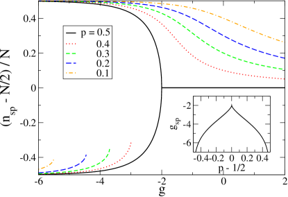
Figure 2: The relation between the saddle point $y_{\rm sp}$ in Eq. (21) and the coupling constant $g$. $\frac{1}{N}(n_{\rm sp}-\frac{N}{2})$ as a function of coupling constant $g$ for different $p$. As $g\leq g_{\rm sp}$, two saddle points arise where $n_{\rm sp,-}<n_{\rm sp,+}$. Inset: $g_{\rm sp}$ as a function of $p-\frac{1}{2}$.

The numerator in Eq. (17) in large $N$ limit can be evaluated by a similar way. In large $N$ limit, $\langle n\rangle=n_{\rm sp}$ if $g>g_{\rm sp}$. When $g<g_{\rm sp}$, we have

$$\langle n\rangle=\left\{\begin{tabular}[]{cc}$n_{\rm sp,+}$&\ \ \ if \ $p<\frac{1}{2}$\\ $\frac{N}{2}$&\ \ \ if \ $p=\frac{1}{2}$\\ $n_{\rm sp,-}$&\ \ \ if \ $p>\frac{1}{2}$\end{tabular}\right.$$ (25)

When $p=\frac{1}{2}$, the system undergoes a second-order phase transition by varying the coupling constant $g$. The order parameter, $\langle n\rangle$, changes continuously across the transition. The critical point $g_{c}$ can be determined by solving $f^{\prime\prime}(x_{\rm sp})|_{g\rightarrow g_{c}^{+}}=0$, which gives $g_{c}=-2$.

If $g<g_{c}$, there’s a first-order phase transition as $p$ varies. The critical point $p_{c}$ is given by $f(x_{\rm sp,+})|_{p\rightarrow p_{c}^{-}}=f(x_{\rm sp,-})|_{p\rightarrow p_{c}^{+}}$, which gives $p_{c}=\frac{1}{2}$. As seen from Eq. (25) and Fig. 3, the order parameter, $\langle n\rangle$, changes discontinuously at $p=p_{c}$. The saddle point at $x_{\rm sp,-}(x_{\rm sp,+})$ when $p<p_{c}(p>p_{c})$ represents the metastable state. Due to the existence of the metastable state, the system shows hysteresis. In the section VI, we provide another means to indicate the existence of metastability.

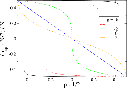
Figure 3: The relation between the saddle point $y_{\rm sp}$ in Eq. (21) and $p$. $\frac{1}{N}(n_{\rm sp}-\frac{N}{2})$ as a function of $p-\frac{1}{2}$ for different $g$.

IV IV. Relaxation to equilibrium

When the system is not at its equilibrium, it will relax. It is interesting to know how the relaxation time behaves. Expanding Eq. (14) with the help of Eq. (15) gives

$$\langle n\rangle_{s} = \langle n\rangle+\lambda_{N-1}^{s}\sum_{n,k=0}^{N}nA_{n,N-1}A_{N-1,k}^{-1}\psi_{k}(0)$$ (26)

$$+\lambda_{N-2}^{s}\sum_{n,k=0}^{N}nA_{n,N-2}A_{N-2,k}^{-1}\psi_{k}(0)$$

$$+\cdots+\lambda_{0}^{s}\sum_{n,k=0}^{N}nA_{n0}A_{0k}^{-1}\psi_{k}(0)$$

where the eigenvalues are arranged in ascending order, $\lambda_{0}<\lambda_{1}<\cdots<\lambda_{N-1}<\lambda_{N}=1$. If $s$ is large enough, the last contribution term before reaching the equilibrium is the $\lambda_{N-1}$ term, which also defines the relaxation time

$$\tau_{\rm R}\equiv-\frac{1}{\ln(\lambda_{N-1})}$$ (27)

If $g=0$, for large $N$, $\tau_{\rm R}=N$. If $g\neq 0$, the eigenvalues can be found by perturbation (See Appendix D for details).

For $g>g_{\rm sp}$, let $M_{0}$ be the transition matrix at $g=0$. The perturbed transition matrix $M_{1}=M-M_{0}$, and then apply Eq. (101), after some algebra, we have the first-order perturbation correction to the $m$-th eigenvalue

$$\lambda_{m}^{(1)} = -\frac{1}{2N}\sum_{n=1}^{N}A^{-1}_{mn}(q(N-n+1)A_{n-1,m}+pnA_{nm})\tanh[\frac{g}{2N}(2n-N-1)]$$ (28)

$$+\frac{1}{2N}\sum_{n=0}^{N-1}A^{-1}_{mn}(q(N-n)A_{nm}+p(n+1)A_{n+1,m})\tanh[\frac{g}{2N}(2n-N+1)]$$

$$= \frac{1}{2N}\sum_{k=0}^{\frac{N}{2}-1}\tanh[\frac{g}{2N}(2k+1)]\left([A^{-1}_{m,\frac{N}{2}-k}-A^{-1}_{m,\frac{N}{2}-k-1}][q(\frac{N}{2}+k+1)A_{\frac{N}{2}-k-1,m}+p(\frac{N}{2}-k)A_{\frac{N}{2}-k,m}]\right.$$

$$\left.+[A^{-1}_{m,\frac{N}{2}+k}-A^{-1}_{m,\frac{N}{2}+k+1}][q(\frac{N}{2}-k)A_{\frac{N}{2}+k,m}+p(\frac{N}{2}+k+1)A_{\frac{N}{2}+k+1,m}]\right)$$

For $m=N$, notice that $A^{-1}_{Nn}=1$ by using Eqs. (68) and (74), we get $\lambda_{N}^{(1)}=0$. It is consistent with the fact that the eigenvalue $\lambda_{N}=1$ for the equilibrium state should be unchanged under perturbation.

The next largest eigenvalue is responsible for the relaxation time to the equilibrium. For $m=N-1$ in Eq. (28), and notice that $A^{-1}_{N-1,n}=qN-n$ and $A_{n,N-1}=\phi_{n}(N)(qN-n)/(Npq)$ which can be obtained from Eqs. (68) and (74), after some algebra, we have

$$\lambda_{N-1}^{(1)} = -\frac{1}{2qN^{2}}\sum_{k=0}^{\frac{N}{2}-1}\frac{N!}{(\frac{N}{2}+k)!(\frac{N}{2}-k)!}p^{\frac{N}{2}+k}q^{\frac{N}{2}-k}(\frac{N}{2}-k)[2k+1+(2q-1)N]\tanh[\frac{g}{2N}(2k+1)]$$ (29)

$$-\frac{1}{2pN^{2}}\sum_{k=0}^{\frac{N}{2}-1}\frac{N!}{(\frac{N}{2}+k)!(\frac{N}{2}-k)!}q^{\frac{N}{2}+k}p^{\frac{N}{2}-k}(\frac{N}{2}-k)[2k+1+(2p-1)N]\tanh[\frac{g}{2N}(2k+1)]$$

$$\simeq -\frac{1}{q}\sqrt{\frac{N}{2\pi pq}}\int_{-\frac{1}{2}(p-q)}^{q}dx{\rm e}^{-\frac{N}{2pq}x^{2}}x(q-x)\tanh[g(x+\frac{1}{2}(p-q))]$$

$$-\frac{1}{p}\sqrt{\frac{N}{2\pi pq}}\int_{-\frac{1}{2}(q-p)}^{p}dx{\rm e}^{-\frac{N}{2pq}x^{2}}x(p-x)\tanh[g(x+\frac{1}{2}(q-p))]$$

$$= -\frac{gpq}{N}{\rm sech}^{2}[\frac{g}{2}(q-p)]+O(N^{-2})$$

where we only keep the leading order for large $N$ in the asymptotic expansion. From the definition of the relaxation time in Eq. (27),

$$\tau_{\rm R}=\frac{2N}{1+2gpq{\rm sech}^{2}[\frac{g}{2}(q-p)]}$$ (30)

In particular, when $p=\frac{1}{2}$,

$$\tau_{\rm R}=\frac{2N}{1+\frac{g}{2}}$$ (31)

Notice that $\tau_{R}\rightarrow 0$ as $g\rightarrow+\infty$. The more repulsive interaction, the shorter relaxation time to the equilibrium.

By keeping only the first two terms in Eq. (26), and using the definition of $\tau_{R}$ from Eq. (27), we have

$$\langle n\rangle_{s}=\langle n\rangle+(n_{0}-\langle n\rangle){\rm e}^{-s/\tau_{\rm R}}$$ (32)

as $s$ is large enough. $n_{0}$ is the initial value. The above formula is compared with the numerical result, as shown in Fig. 4. Good agreement at large $s$ is found.

For $g<g_{\rm sp}$, let $M_{0}$ be the transition matrix at $g\rightarrow-\infty$. Without loss of generality, suppose $p\leq\frac{1}{2}$, then the equilibrium eigenstate is labelled by $m=N$, of eigenvalue $\lambda_{N}^{(0)}=1$. The eigenstate of the next largest eigenvalue is labelled by $m=N-1$, of eigenvalue $\lambda_{N-1}^{(0)}=1-\frac{p}{N}$.

By Eq. (101), and notice that the non-vanishing $A_{nN}=1$ for $n=N$, $A_{n,N-1}=(-1)^{n}$ for $n\geq N-1$ from Eq. (81), we get $\lambda_{N}^{(1)}=(M_{1})_{NN}+(M_{1})_{N-1,N}=0$, which is again consistent with $\lambda_{N}=1$ unchanged under perturbation.

The first-order perturbation correction to the next largest eigenvalue is

$$\lambda_{N-1}^{(1)} = -(M_{1})_{N-1,N}+(M_{1})_{N-1,N-1}+2(M_{1})_{N-2,N-1}$$ (33)

$$= -\frac{qN-p}{N}\frac{1}{{\rm e}^{|g|(1-\frac{1}{N})}+1}+\frac{q(N-1)}{N}\frac{1}{{\rm e}^{|g|(1-\frac{3}{N})}+1}$$

$$= \frac{1}{N}\left(\frac{|g|q}{2}{\rm sech}^{2}(\frac{|g|}{2})+\frac{p-q}{{\rm e}^{|g|}+1}\right)+O(N^{-2})$$

if only the leading order for large $N$ is kept. The relaxation time is then

$$\tau_{\rm R}=\frac{N}{p-\frac{|g|q}{2}{\rm sech}^{2}(\frac{|g|}{2})-\frac{p-q}{{\rm e}^{|g|}+1}}$$ (34)

$g$ is largely negative if $p$ deviates from $\frac{1}{2}$ a lot, as shown in the inset of Fig. 2. In this case, $\tau_{\rm R}\simeq\frac{N}{p}$, which is the limit as $g\rightarrow-\infty$.

Similarly, if $p>\frac{1}{2}$, the relaxation time is

$$\tau_{\rm R}=\frac{N}{q-\frac{|g|p}{2}{\rm sech}^{2}(\frac{|g|}{2})-\frac{q-p}{{\rm e}^{|g|}+1}}$$ (35)

and $\tau_{\rm R}\simeq\frac{N}{q}$ when $p$ deviates from $\frac{1}{2}$ a lot.

With the help of the relaxation time, we have

$$\langle|n-n_{0}|\rangle_{s}+n_{0}=\langle n\rangle+(n_{0}-\langle n\rangle){\rm e}^{-s/\tau_{\rm R}}$$ (36)

as $s$ is large enough. $n_{0}$ is the initial value. Here we use $\langle|n-n_{0}|\rangle_{s}+n_{0}$ instead of $\langle n\rangle_{s}$ in order to avoid the interference from the metastable state. The above formula is compared with the numerical result, as shown in Fig. 5. Again both analytical and numerical results match well at large $s$.

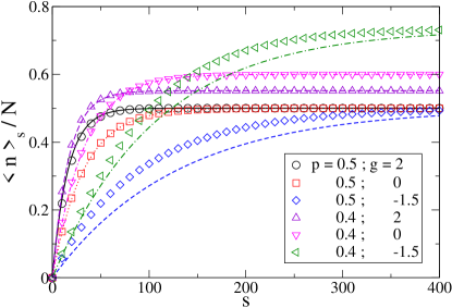
Figure 4: The proportion of particle number in the left urn, $\langle n\rangle_{s}/N$, as a function of time step $s$ for $g>g_{\rm sp}$ at different $p$ and $g$. The initial value $n_{0}$ is chosen to be the most far-from-equilibrium state. Solid lines represent the corresponding result by Eq. (32).

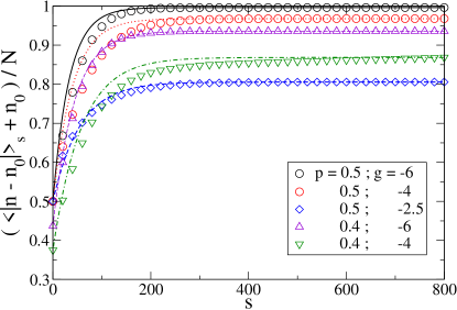
Figure 5: The proportion of particle number in the left urn, $(\langle|n-n_{0}|\rangle_{s}+n_{0})/N$, as a function of time step $s$ for $g<g_{\rm sp}$ at different $p$ and $g$. The initial value $n_{0}$ is chosen to be the most far-from-equilibrium state. Solid lines represent the corresponding result by Eq. (36).

V V. Poincare cycle

In this section, we are going to discuss the scaling behavior of the Poincare cycle with respect to the particle number $N$ and the tuning parameters ($g$ or $p$) across the (first-order and second-order) phase transition.

The Poincare cycle of the state $|n\rangle$, denoted by $\tau_{\rm P}(n)$, is defined as the mean time from the state $|n\rangle$ to its original state at its first time, $\tau(n\rightarrow n)$, which is (see Appendix C for the proof)

$$\tau_{\rm P}(n)=\frac{\sum_{k=0}^{N}\phi_{k}(N)}{\phi_{n}(N)}$$ (37)

If $p=\frac{1}{2}$, by Eqs. (13) and (20), and also notice that $f^{\prime\prime}(x_{\rm sp})=-2(g-g_{c})$ with $g_{c}=-2$, it is straightforward to have the Poincare cycle of the equilibrium

$$\tau_{\rm P}^{\rm eq}=\tau_{\rm P}(n_{\rm sp})=\sqrt{\pi}(g-g_{c})^{-\frac{1}{2}}N^{\frac{1}{2}}$$ (38)

If $g<g_{c}$, two saddle points $n_{{\rm sp},\pm}$ emerge. When $g\lesssim g_{c}$, $n_{{\rm sp},+}\gtrsim\frac{N}{2}$ and $n_{{\rm sp},-}\lesssim\frac{N}{2}$. $f(x_{{\rm sp},+})=f(x_{{\rm sp},-})$. One can solve for $x_{{\rm sp},\pm}\simeq\frac{1}{2}\pm\sqrt{\frac{3}{8}}(g_{c}-g)^{\frac{1}{2}}$. Notice that $f^{\prime\prime}(x_{{\rm sp},\pm})=-4(g_{c}-g)$, the Poincare cycle of the equilibrium

$$\tau_{\rm P}^{\rm eq}=\sqrt{2\pi}(g_{c}-g)^{-\frac{1}{2}}N^{\frac{1}{2}}$$ (39)

When $g\ll g_{c}$, $n_{{\rm sp},+}\lesssim N$ and $n_{{\rm sp},-}\gtrsim 0$, then $x_{{\rm sp},+}\simeq 1-{\rm e}^{g}$, and $x_{{\rm sp},-}\simeq{\rm e}^{g}$. $f^{\prime\prime}(x_{{\rm sp},\pm})\simeq-{\rm e}^{-g}$, then

$$\tau_{\rm P}^{\rm eq}=2\sqrt{2\pi}{\rm e}^{-\frac{|g|}{2}}N^{\frac{1}{2}}$$ (40)

The Poincare cycle of the equilibrium state $\tau_{\rm P}^{\rm eq}$ has always $\sqrt{N}$ dependence. It becomes divergent at the transition point $g=g_{c}$. From Eq. (20), it is seen that the divergence comes from the vanishing $|f^{\prime\prime}(x_{\rm sp})|_{g\rightarrow g_{c}}$ in the denominator, which implies that it is universal in second-order phase transition. However, note that Eq. (20) is obtained in large $N$ limit. For large but finite $N$, one should see the divergent-like scaling behavior instead of real divergence.

Next we investigate the scaling behavior of the Poincare cycle of the most far-from-equilibrium state $\tau_{\rm P}^{\rm feq}$, in which it is defined as the longest Poincare cycle.

When $p=\frac{1}{2}$, and $g>g_{c}$, then $n_{\rm sp}=\frac{N}{2}$, the most far-from-equilibrium state is at $n=N$ (or $n=0$), then

$$\tau_{\rm P}^{\rm feq}=\tau_{\rm P}(N)=\sqrt{2}(g-g_{c})^{-\frac{1}{2}}\exp[N(\ln 2+\frac{g}{4})]$$ (41)

If $g\lesssim g_{c}$,

$$\tau_{\rm P}^{\rm feq}=\tau_{\rm P}(N)=2(g_{c}-g)^{-\frac{1}{2}}\exp[N(\ln 2+\frac{g}{4})]$$ (42)

If $g\ll g_{c}$,

$$\tau_{\rm P}^{\rm feq}=\tau_{\rm P}(\frac{N}{2})=\sqrt{2\pi}N^{\frac{1}{2}}\exp[N(\frac{|g|}{4}-\ln 2)]$$ (43)

The Poincare cycle of the most far-from-equilibrium $\tau_{\rm P}^{\rm feq}$ has the exponential form ${\rm e}^{\alpha N}$. It also becomes “divergent” (see the argument above) at $g=g_{c}$, but the scaling exponent $\alpha$ is finite and continuous across the transition point.

In the following, we are going to investigate the behavior of the Poincare cycle across the first-order phase transition. Suppose $g\ll g_{\rm sp}$, there are two saddle points. When $p<p_{c}=\frac{1}{2}$, $x_{\rm sp,+}\simeq 1-(1+\ln\frac{p}{q}){\rm e}^{g}$ and $x_{\rm sp,-}\simeq(1-\ln\frac{p}{q}){\rm e}^{g}$, the Poincare cycle of the equilibrium state

$$\tau_{\rm P}^{\rm eq}=\tau_{\rm P}(n_{\rm sp,+})=\sqrt{2\pi}{\rm e}^{-\frac{|g|}{2}}N^{\frac{1}{2}}\left(1+\ln\left(\frac{p}{q}\right)\right)^{\frac{1}{2}}$$ (44)

When $p>p_{c}$, $x_{\rm sp,+}\simeq 1-(1+\ln\frac{q}{p}){\rm e}^{g}$, $x_{\rm sp,-}\simeq(1-\ln\frac{q}{p}){\rm e}^{g}$, then

$$\tau_{\rm P}^{\rm eq}=\tau_{\rm P}(n_{\rm sp,-})=\sqrt{2\pi}{\rm e}^{-\frac{|g|}{2}}N^{\frac{1}{2}}\left(1+\ln\left(\frac{q}{p}\right)\right)^{\frac{1}{2}}$$ (45)

It is interesting to notice that $\tau_{\rm P}^{\rm eq}\simeq\sqrt{2\pi}|g|^{-\frac{1}{2}}N^{\frac{1}{2}}$ if $p\neq p_{c}$. At the transition point $p=p_{c}$, $\tau_{\rm P}^{\rm eq}=2\sqrt{2\pi}|g|^{-\frac{1}{2}}N^{\frac{1}{2}}$. The Poincare cycle of the equilibrium state is finite and continuous during first-order transition.

The most far-from-equilibrium state is at $n=N(\frac{1}{2}-\ln(\frac{p}{q}){\rm e}^{g})$, then

$$\tau_{\rm P}^{\rm feq}= \sqrt{\frac{\pi}{2}}N^{\frac{1}{2}}\exp[N(\frac{|g|}{4}-\ln 2)]$$ (46)

$$\times\left(\left(\frac{p}{q}\right)^{\frac{N}{2}}+\left(\frac{q}{p}\right)^{\frac{N}{2}}\right)$$

When $p$ is around the transition point $p_{c}$, in large $N$ limit, $\tau_{\rm P}^{\rm feq}=\sqrt{\frac{\pi}{2}}N^{\frac{1}{2}}\exp[N(\frac{|g|}{4}-\ln 2)]$. At exactly $p=p_{c}$, $\tau_{\rm P}^{\rm feq}$ is double its value.

The Poincare cycle of the most far-from-equilibrium has still the exponential form ${\rm e}^{\alpha N}$ dependence, with a continuous exponent $\alpha$ across the first-order phase transition.

In summary, the Poincare cycles $\tau_{\rm P}^{\rm eq}$ and $\tau_{\rm P}^{\rm feq}$ have the $\sqrt{N}$ and ${\rm e}^{\alpha N}$ dependence, respectively. During second-order phase transition, both $\tau_{\rm P}^{\rm eq}$ and $\tau_{\rm P}^{\rm feq}$ behave divergent-like at the transition point. At first-order phase transition, the Poincare cycles are finite and continuous. Such a behavior of the Poincare cycle could be served as an indication of the nature of the phase transition

VI VI. Duration Time

When $g\ll g_{\rm sp}$, the system will stay at the states $|0\rangle$ and $|N\rangle$. Suppose the system transits from $|N\rangle$ to $|0\rangle$, it should meet $|\frac{N}{2}\rangle$ during the evolution because $n$ changes continuously (Here the continuity of $n$ means $n$ changes its value at most $\pm 1$ at each step).

Define $\tau_{\rm D}(n,1)$ as the mean time for the system to evolve from $|\frac{N}{2}\rangle$ to $|n\rangle$ at its first time, and then back $|\frac{N}{2}\rangle$ at its first time. When $n=N$,

$$\tau_{\rm D}(N,1)\equiv\sum_{s_{1}=1}^{\infty}\sum_{s_{2}=1}^{\infty}(s_{1}+s_{2})(\frac{N}{2}|p(s_{2})|N)(N|p(s_{1})|\frac{N}{2})$$

where the notation $(m|p(s)|n)$ represents the probability that the state $|m\rangle$ becomes $|n\rangle$ at its first time after $s$ steps. With the help of Eqs. (95-97), Eq. (VI) becomes

$$\tau_{\rm D}(N,1) = \tau(\frac{N}{2}\rightarrow N)g_{\frac{N}{2},N}(1)+\tau(N\rightarrow\frac{N}{2})g_{N,\frac{N}{2}}(1)$$ (48)

$$= \tau_{\rm P}(N)+\tau_{\rm P}(\frac{N}{2})$$

Since $\tau_{\rm P}(\frac{N}{2})\gg\tau_{\rm P}(N)$ for $g\ll g_{\rm sp}$, $\tau_{\rm D}(N,1)=\tau_{\rm P}(\frac{N}{2})$. By similar argument, $\tau_{\rm D}(0,1)=\tau_{\rm P}(\frac{N}{2})$.

The above transition ( $|\frac{N}{2}\rangle\rightarrow|n\rangle\rightarrow|\frac{N}{2}\rangle$ ) may occur $k$ times consecutively. Define $\tau_{\rm D}(n,k)$ as its mean time, then

$$\tau_{\rm D}(n,k) \equiv \sum_{s_{1},\ldots,s_{2k}=1}^{\infty}(s_{1}+s_{2}+\ldots+s_{2k})(\frac{N}{2}|p(s_{2k}|n)(n|p(s_{2k-1})|\frac{N}{2})\cdots(\frac{N}{2}|p(s_{2})|n)(n|p(s_{1})|\frac{N}{2})$$ (49)

$$= k\sum_{s=1}^{\infty}s(n|p(s)|\frac{N}{2})+k\sum_{s=1}^{\infty}s(\frac{N}{2}|p(s)|n)$$

$$= k\left(\tau_{\rm P}(n)+\tau_{\rm P}(\frac{N}{2})\right)$$

Hence $\tau_{\rm D}(N,k)=\tau_{\rm D}(0,k)=k\tau_{\rm P}(\frac{N}{2})$.

The duration time at state $|N\rangle$, $\tau_{D}(N)$, defined as the total time at which the system stays at $|N\rangle$ before transits to $|0\rangle$,

$$\tau_{\rm D}(N) \equiv \sum_{k=1}^{\infty}\left(\frac{\tau_{\rm P}(N)^{-1}}{\tau_{\rm P}(N)^{-1}+\tau_{\rm P}(0)^{-1}}\right)^{k}\tau_{\rm D}(N,k)$$

$$= \left(\tau_{\rm P}(N)+\tau_{\rm P}(\frac{N}{2})\right)\sum_{k=1}^{\infty}k\left(\frac{p^{N}}{p^{N}+q^{N}}\right)^{k}$$

$$= \left(\frac{q}{p}\right)^{N}\left[\left(\frac{q}{p}\right)^{N}+1\right]\left(\tau_{\rm P}(N)+\tau_{\rm P}(\frac{N}{2})\right)$$

The asymptotic form at large $N$ limit becomes

$$\tau_{\rm D}(N)=\left\{\begin{tabular}[]{cc}$(\frac{q}{p})^{2N}\tau_{\rm P}(\frac{N}{2})$&\ \ \ if \ $p<\frac{1}{2}$\\ $2\tau_{\rm P}(\frac{N}{2})$&\ \ \ if \ $p=\frac{1}{2}$\\ $(\frac{q}{p})^{N}\tau_{\rm P}(\frac{N}{2})$&\ \ \ if \ $p>\frac{1}{2}$\\ \end{tabular}\right.$$ (54)

Similarly, the duration time at state $|0\rangle$ is

$$\tau_{\rm D}(0)=\left(\frac{p}{q}\right)^{N}\left[\left(\frac{p}{q}\right)^{N}+1\right]\left(\tau_{\rm P}(0)+\tau_{\rm P}(\frac{N}{2})\right)$$

and its asymptotic form

$$\tau_{\rm D}(0)=\left\{\begin{tabular}[]{cc}$(\frac{p}{q})^{N}\tau_{\rm P}(\frac{N}{2})$&\ \ \ if \ $p<\frac{1}{2}$\\ $2\tau_{\rm P}(\frac{N}{2})$&\ \ \ if \ $p=\frac{1}{2}$\\ $(\frac{p}{q})^{2N}\tau_{\rm P}(\frac{N}{2})$&\ \ \ if \ $p>\frac{1}{2}$\\ \end{tabular}\right.$$ (59)

There is a first-order phase transition as $p$ varies. As $p<p_{c}$, $\tau_{\rm D}(N)>\tau_{\rm D}(0)>0$. It means the state $|N\rangle$ is preferable but $|0\rangle$ still survives. Upon increasing $p$, the ratio of the duration time of two states, $\tau_{\rm D}(N)/\tau_{\rm D}(0)$, decreases. At $p=p_{c}$, $\tau_{\rm D}(N)=\tau_{\rm D}(0)$. Further increasing $p>p_{c}$, $\tau_{\rm D}(0)>\tau_{\rm D}(N)>0$. Such a behavior indicates a strong evidence of metastability during first-order phase transition.

VII VII. Discussion

The order-of-magnitude determination of the Poincare cycle of the most far-from-equilibrium state was originally used to resolve the recurrence paradox. In macroscopic world, it is far beyond the time scale we can observe. If $N$ is not large enough, in principle, the measurement of the Poincare cycle should be experimentally accessible. For example, in colloidal system, one can easily prepare the system of small particle number $N$. The interaction between the colloidal particles ($g$ in our model) is also well controlled yethiraj . The probability of directed transport ($p$ in our model) can be tuned by applying the electric field along the direction from the left to the right urn, and the particles are slightly charged.

VIII acknowledgement

One of the authors (C.H.C.) thanks Pik-Yin Lai and Chi-Ning Chen for their helpful discussion. The work was supported by the Ministry of Science and Technology of the Republic of China.

*

Appendix A Appendix A: Eigenproblem for $g=0$

The standard way to solve the eigenproblem is the method of generating functions feller . For $g=0$, it was already known siegert ; klein ; lee . In the following, we briefly outline the solution.

For $g=0$, Eq. (II) is reduced to

$$\frac{N-n+1}{2N}q\phi_{n-1}+\frac{n+1}{2N}p\phi_{n+1}+\left(1-\frac{n}{2N}p-\frac{N-n}{2N}q\right)\phi_{n}=\lambda\phi_{n}$$ (60)

Let $f(z)\equiv\sum_{n=0}^{N}\phi_{n}z^{n}=\sum_{n=-\infty}^{\infty}\phi_{n}z^{n}$, if we extend $\phi_{n}\equiv 0$ for $n<0$ and $n>N$, then

$$\frac{1}{N}\frac{df}{dz}(p+qz)(1-z)=(2\lambda-1-(p+qz))f$$ (61)

The solution is

$$f(z)=(p+qz)^{N(2\lambda-1)}(1-z)^{2N(1-\lambda)}$$ (62)

up to an arbitrary proportional constant. Since $f(z)$ is a polynomial in $z$ by definition, $N(2\lambda-1)$ and $2N(1-\lambda)$ have to be non-negative integers. Hence we get

$$\lambda_{m}=\frac{1}{2}+\frac{m}{2N}$$ (63)

where $m=0,1,2,\ldots,N$ are the numbers to label the eigenvalues. The corresponding eigenvectors of the component $\phi_{n}(m)$ could be obtained by comparing the $z^{n}$ coefficient of $f(z)$ in Eq. (62) with its definition, we have

$$\phi_{n}(m)=\sum_{k+l=n}\left(\begin{array}[]{c}m\\ k\\ \end{array}\right)\left(\begin{array}[]{c}N-m\\ l\\ \end{array}\right)(-1)^{l}p^{m-k}q^{k}$$ (68)

In particular, for $\lambda_{N}=1$, its corresponding eigenvector

$$\phi_{n}(N)=\frac{N!}{n!(N-n)!}p^{N-n}q^{n}$$ (70)

Now $A_{nm}=\phi_{n}(m)$, its inverse $A_{nm}^{-1}$ is defined as

$$\sum_{n}A_{ln}A_{nm}^{-1}=\delta_{lm}$$ (71)

Multiply $z^{l}$, sum over $l$, and make use of Eq.(62-63), we get

$$\sum_{n}(p+qz)^{n}(1-z)^{N-n}A_{nm}^{-1}=z^{m}$$ (72)

By change of variable $t=-\frac{p+qz}{1-z}$, we have

$$\sum_{n}A_{nm}^{-1}(-1)^{m+n}t^{n}=q^{N-m}f_{m}(\frac{t}{q})$$ (73)

which gives

$$A_{nm}^{-1}=(-1)^{m+n}q^{N-m-n}\phi_{n}(m)$$ (74)

Appendix B Appendix B: Eigenproblem for $g\rightarrow-\infty$

As $g\rightarrow-\infty$, Eq. (II) is reduced to

$$\frac{N-n+1}{N}q\Theta(n-\frac{N+1}{2})\phi_{n-1}+\frac{n+1}{N}p\Theta(\frac{N-1}{2}-n)\phi_{n+1}$$

$$+\left(1-\frac{n}{N}p\Theta(\frac{N+1}{2}-n)-\frac{N-n}{N}q\Theta(n-\frac{N-1}{2})\right)\phi_{n}=\lambda\phi_{n}$$ (75)

where $\Theta(x)$ is the step function. When $n=\frac{N}{2}$, it becomes $\frac{1}{2}\phi_{\frac{N}{2}}=\lambda\phi_{\frac{N}{2}}$. Hence $\lambda_{\frac{N}{2}}=\frac{1}{2}$, and the corresponding eigenvector is $\phi(\frac{N}{2})=(0,\ldots,1,\ldots,0)^{T}$ with the only non-vanishing component $\phi_{\frac{N}{2}}(\frac{N}{2})=1$ (Here we label this eigenstate by $\frac{N}{2}$ ). The matrix $M$ is in block diagonal form. We first search for the eigenstates such that $\phi_{n}=0$ for $n\geq\frac{N}{2}$, and further assume that $\phi_{n}\equiv 0$ for $n<0$. Let $f(z)\equiv\sum_{n=0}^{N}\phi_{n}z^{n}=\sum_{n=-\infty}^{\infty}\phi_{n}z^{n}$, then

$$\frac{p}{N}\frac{df}{dz}(1-z)=(\lambda-1)f$$ (76)

The solution is

$$f(z)=(1-z)^{N(1-\lambda)/p}$$ (77)

up to an arbitrary proportional constant. Since $f(z)$ is a polynomial of degree $\frac{N}{2}-1$ in $z$ by definition, $N(1-\lambda)/p$ have to be non-negative integers less than or equal to $\frac{N}{2}-1$. Hence we get

$$\lambda_{m}=1-p\frac{N-m}{N}$$ (78)

where $m=\frac{N}{2}+1,\ldots,N-1,N$ are the numbers to label the eigenvalues. The non-vanishing components of the corresponding eigenvectors are

$$\phi_{n}(m)=(-1)^{n}\left(\begin{array}[]{c}N-m\\ N-n\\ \end{array}\right)$$ (81)

which are the $z^{N-n}$ coefficient of $f_{m}(z)=(1-z)^{N-m}$ with $\frac{N}{2}+1\leq m\leq n\leq N$.

By making the transformation from $n$ to $N-n$ and $p$ to $1-p$ in Eq.(75), we get another set of eigenstates such that

$$\phi_{n}(m)=\phi_{N-n}(N-m)$$ (82)

where $m=0,1,\ldots,\frac{N}{2}-1$. With the help of Eq.(78-81), the non-vanishing components of the eigenvectors are

$$\phi_{n}(m)=(-1)^{n}\left(\begin{array}[]{c}m\\ n\\ \end{array}\right)$$ (85)

where $0\leq n\leq m\leq\frac{N}{2}-1$, $f_{m}(z)=(1-z)^{m}$, and the corresponding eigenvalues are

$$\lambda_{m}=1-q\frac{m}{N}$$ (86)

Now the matrix $A_{nm}=\phi_{n}(m)$ is block diagonal with three blocks, $\{A_{nm}\}_{0\leq n,m\leq\frac{N}{2}-1}$, $A_{\frac{N}{2},\frac{N}{2}}$, and $\{A_{nm}\}_{\frac{N}{2}+1\leq n,m\leq N}$. We first restrict the upper block, its inverse $A_{nm}^{-1}$ is defined as

$$\sum_{n=0}^{\frac{N}{2}-1}A_{ln}A_{nm}^{-1}=\delta_{lm}$$ (87)

Similar to the treatment for the case that $g=0$, multiply $z^{l}$, sum over $l$, make use of Eq. (85-86), and then make the change of variable $t=1-z$, we arrive at

$$\sum_{n=0}^{\frac{N}{2}-1}A_{nm}^{-1}t^{n}=f_{m}(t)$$ (88)

which gives

$$A_{nm}^{-1}=\phi_{n}(m)$$ (89)

where $0\leq n,m\leq\frac{N}{2}-1$. Eq. (89) also holds for $0\leq n,m\leq N$. By the symmetry argument as above, the transformation $n\rightarrow N-n$, $p\rightarrow 1-p$ leaves Eq. (75) unchanged, Eq. (89) should hold for $\frac{N}{2}+1\leq n,m\leq N$. It’s also straightforward to check $A_{\frac{N}{2},\frac{N}{2}}^{-1}=A_{\frac{N}{2},\frac{N}{2}}=\phi_{\frac{N}{2}}(\frac{N}{2})=1$, which is Eq. (89) with $n=m=\frac{N}{2}$.

Appendix C Appendix C: Mean Time from state to state

Denote $(n|p(s)|m)$ as the probability that the state $|m\rangle$ becomes the state $|n\rangle$ at its first time after $s$ steps. It’s relation with the probability $\langle n|p(s)|m\rangle$ is

$$\langle n|p(s)|m\rangle=(n|p(s)|m)+\sum_{k=1}^{s-1}\langle n|p(s-k)|n\rangle(n|p(k)|m)$$

Define two generating functions,

$$h_{mn}(z) \equiv \sum_{s=1}^{\infty}\langle n|p(s)|m\rangle z^{s}$$ (91)

$$= \sum_{s=1}^{\infty}(M^{s})_{nm}z^{s}$$

$$= \sum_{s=1}^{\infty}\sum_{k=0}^{N}A_{nk}\lambda_{k}^{s}A_{km}^{-1}z^{s}$$

$$= \sum_{k=0}^{N}A_{nk}A_{km}^{-1}\frac{\lambda_{k}z}{1-\lambda_{k}z}$$

and

$$g_{nm}(z) \equiv \sum_{s=1}^{\infty}(n|p(s)|m)z^{s}$$ (92)

We can deduce the relation between these two generating functions from Eq. (C).

$$h_{mn}(z)=g_{nm}(z)+h_{nn}(z)g_{nm}(z)$$ (93)

or equivalently,

$$g_{mn}(z)=\frac{h_{nm}(z)}{h_{nn}(z)+1}$$ (94)

The probability normalization

$$\sum_{s=1}^{\infty}(n|p(s)|m)=g_{nm}(1)=\lim_{z\rightarrow 1^{-}}\frac{h_{nm}(z)}{h_{nn}(z)+1}=\frac{A_{nN}A_{Nm}^{-1}}{A_{nN}A_{Nn}^{-1}}=1$$ (95)

Here we use the fact that $A_{Nk}^{-1}$ is independent of $k$, and we label $\lambda_{N}=1$.

The mean time from the state $|m\rangle$ to the state $|n\rangle$ at its first time is defined as

$$\tau(m\rightarrow n)\equiv\sum_{s=1}^{\infty}s(n|p(s)|m)=\left.\frac{dg_{nm}}{dz}\right|_{z=1}=\frac{A_{nN}A_{Nm}^{-1}}{(A_{nN}A_{Nn}^{-1})^{2}}=\frac{\sum_{k=0}^{N}\phi_{k}(N)}{\phi_{n}(N)}$$ (96)

Note that the mean time is independent of the initial state $|m\rangle$. The Poincare cycle $\tau_{\rm P}(n)$, defined as $\tau(n\rightarrow n)$, also shares the same result,

$$\tau_{\rm P}(n)=\frac{\sum_{k=0}^{N}\phi_{k}(N)}{\phi_{n}(N)}$$ (97)

Appendix D Appendix D: Perturbation Theory

We want to solve the eigenproblem

$$M\phi(m)=\lambda_{m}\phi(m)$$ (98)

Suppose the eigenproblem $M_{0}\phi^{(0)}(m)=\lambda_{m}^{(0)}\phi^{(0)}(m)$ are solved. Let the matrix $A_{nm}=\phi^{(0)}_{n}(m)$, $\psi^{(0)}(m)=A^{-1}\phi^{(0)}(m)$, then

$$\Lambda_{0}\psi^{(0)}(m)=\lambda_{m}^{(0)}\psi^{(0)}(m)$$ (99)

where $(\Lambda_{0})_{nm}=\lambda_{m}^{(0)}\delta_{nm}$ and $\psi_{n}^{(0)}(m)=\delta_{nm}$. It is obvious to see the orthnormality relation $\psi^{(0)T}(n)\psi^{(0)}(m)=\delta_{nm}$.

Write $M=M_{0}+M_{1}$ and $\phi(m)=\phi^{(0)}(m)+\phi^{(1)}(m)$. Keep Eq. (98) up to the first order, we have

$$(\Lambda_{1}-\lambda_{m}^{(1)})\psi^{(0)}(m)=(\lambda_{m}^{(0)}-\Lambda_{0})\psi^{(1)}(m)$$ (100)

where $\Lambda_{1}=A^{-1}M_{1}A$ and $\psi^{(1)}(m)=A^{-1}\phi^{(1)}(m)$. Multiply both sides of Eq. (100) by $\psi^{(0)T}(m)$, then we get the first order correction of eigenvalue

$$\lambda_{m}^{(1)}=(\Lambda_{1})_{mm}=(A^{-1}M_{1}A)_{mm}$$ (101)

References

(1)
K. Huang, Statistical Mechanics, 2nd ed. (Wiley, 1987).
(2)
H. Poincare, Acta Math. 13, 1 (1892).
(3)
P. Ehrenfest and T. Ehrenfest, Phys. Z. 8, 311 (1907).
(4)
M. Kac, Am. Math. Mon. 54, 369 (1947).
(5)
A.J.F. Siegert, Phys. Rev. 76, 1708 (1949).
(6)
M.J. Klein, Phys. Rev. 103, 17 (1956).
(7)
Y.M. Kao and P.G. Luan, Phys. Rev. E67, 031101 (2003).
(8)
Y.M. Kao, Phys. Rev. E69, 027103 (2004).
(9)
J. Nagler, Phys. Rev. E72, 056129 (2005).
(10)
J. Clark, M. Kiwi, F. Torres, J. Rogan, and J.A. Valdivia, Phys. Rev. E92, 012103 (2015).
(11)
Ch. Hauert, J. Nagler, and H.G. Schuster, J. Stat. Phys. 116, 1453 (2004).
(12)
B. Bakar and U. Tirnakli, Phys. Rev. E79, 040103(R) (2009).
(13)
B. Bakar and U. Tirnakli, Physica A 389, 3382 (2010).
(14)
A. Lipowski and M. Droz, Phys. Rev. E65, 031307 (2002).
(15)
A. Lipowski and M. Droz, Phys. Rev. E66, 016118 (2002).
(16)
F. Coppex, M. Droz, and A. Lipowski, Phys. Rev. E66, 011305 (2002).
(17)
G.M. Shim, B.Y. Park, and H. Lee, Phys. Rev. E67, 011301 (2003).
(18)
J. Nagler, C. Hauert, and H.G. Schuster, Phys. Rev. E60, 2706
(1999).