Local Private Hypothesis Testing: Chi-Square Tests

Abstract

The local model for differential privacy is emerging as the reference model for practical applications of collecting and sharing sensitive information while satisfying strong privacy guarantees. In the local model, there is no trusted entity which is allowed to have each individual’s raw data as is assumed in the traditional curator model for differential privacy. Individuals’ data are usually perturbed before sharing them. We explore the design of private hypothesis tests in the local model, where each data entry is perturbed to ensure the privacy of each participant. Specifically, we analyze locally private chi-square tests for goodness of fit and independence testing, which have been studied in the traditional, curator model for differential privacy.

1 Introduction

Hypothesis testing is a widely applied statistical tool used to test whether given models should be rejected, or not, based on sampled data from a population. Hypothesis testing was initially developed for scientific and survey data, but today it is also an essential tool to test models over collections of social network, mobile, and crowdsourced data (American Statistical Association, 2014; Hunter et al., 2008; Steele et al., 2017). Collected data samples may contain highly sensitive information about the subjects, and the privacy of individuals can be compromised when the results of a data analysis are released. In work from Homer et al. (2008), it was shown that a subject in a dataset can be identified as being in the case or control group based on the aggregate statistics of a genetic-wide association study (GWAS). Privacy-risks may bring data contributors to opt out, which reduces the confidence in the data study. A way to address this concern is by developing new techniques to support privacy-preserving data analysis. Among the different approaches, differential privacy (Dwork et al., 2006b) has emerged as a viable solution: it provides strong privacy guarantees and it allows to release accurate statistics. A standard way to achieve differential privacy is by injecting some statistical noise in the computation of the data analysis. When the noise is carefully chosen, it helps to protect the individual privacy without compromising the utility of the data analysis. Several recent works have studied differentially private hypothesis tests that can be used in place of the standard, non-private hypothesis tests (Uhler et al., 2013; Yu et al., 2014; Sheffet, 2015; Karwa and Slavković, 2016; Wang et al., 2015; Gaboardi et al., 2016; Kifer and Rogers, 2017; Cai et al., 2017). These tests work in the curator model of differential privacy. In this model, the data is centrally stored and the curator carefully injects noise in the computation of the data analysis in order to satisfy differential privacy.

In this work we instead address the local model of privacy, formally introduced by Raskhodnikova et al. (2008). The first differentially private algorithm called randomized response – in fact it predates the definition of differential privacy by more than 40 years – guarantees differential privacy in the local model (Warner, 1965). In this model, there is no trusted centralized entity which is responsible for the noise injection. Instead, each individual adds enough noise to guarantee differential privacy for their own data, which provides a stronger privacy guarantee when compared to traditional differential privacy. The data analysis is then run over the collection of the individually sanitized data. The local model of differential privacy is a convenient model for several applications: for example it is used to collect statistics about the activity of the Google Chrome Web browser users (Erlingsson et al., 2014), and to collect statistics about the typing patterns of Apple’s iPhone users (Apple Press Info, 2016). Despite these applications, the local model has received far less attention than the more standard centralized curator model. This is in part due to the more firm requirements imposed by this model, which make the design of effective data analysis harder.

Our main contribution is in designing chi-square hypothesis tests for the local model of differential privacy. Similar to previous works we focus on goodness of fit and independence hypothesis tests. Most of the differentially private chi-square hypothesis tests proposed so far are based on mechanisms that add noise in some form to the aggregate data, e.g. the cells of the contingency tables, or the resulting chi-square statistics value. These approaches cannot be used in the local model, since noise needs to be added at the individual’s data level. We then consider instead general privatizing techniques in the local model, and we study how to build new hypothesis tests with them. Each test we present is characterized by a specific local model mechanism. The main technical challenge for designing each test is to create statistics, which incorporate the local model mechanisms, that converge as we collect more data to a chi-square distribution, as in the classical chi-square tests. We then use these statistics to find the critical value to correctly bound the Type I error.

We present three different goodness of fit tests: LocalNoiseGOF presents a statistic that guarantees the convergence to a chi-square distribution under the null hypothesis so that we can use the correct critical values when local (concentrated) differential privacy is guaranteed by adding Laplace or Gaussian noise to the individual data; LocalExpGOF also provides a statistic that converges to a chi-square under the null hypothesis when a private value for each individual is selected by using the exponential mechanism (McSherry and Talwar, 2007); finally, LocalBitFlipGOF introduces a statistic that converges to a chi-square distribution when the data is privatized using a bit flipping algorithm (Bassily and Smith, 2015), which provide better accuracy for higher dimensional data. Further, we develop corresponding independence tests: LocalNoiseIND, LocalExpIND, and LocalBitFlipIND. For all these tests we study their asymptotic behavior. A desiderata for private hypothesis tests is to have a guaranteed upper bound on the probability of a false discovery (or Type I error) – rejecting a null hypothesis or model when the data was actually generated from it – and to minimize the probability of a Type II error, which is failing to reject the null hypothesis when the model is indeed false. This latter criteria corresponds to the power of the statistical test. We then present experimental results showing the power of the different tests which demonstrates that no single local differentially private algorithm is best across all data dimensions and privacy parameter regimes.

2 Related Works

There have been several works in developing private hypothesis test for categorical data, but all look at the traditional model of (concentrated) differential privacy instead of the local model, which we consider here. Several works have explored private statistical inference for GWAS data, (Uhler et al., 2013; Yu et al., 2014; Johnson and Shmatikov, 2013). Following these works, there has also been general work in private chi-square hypothesis tests, where the main tests are for goodness of fit and independence testing, although some do extend to more general tests (Wang et al., 2015; Gaboardi et al., 2016; Kifer and Rogers, 2017; Cai et al., 2017; Kakizaki et al., 2017). Among these, the works most related to ours are the ones by (Gaboardi et al., 2016; Kifer and Rogers, 2017). We will compare our work with these in Section 4 after introducing them. There has also been work in private hypothesis testing for ordinary least squares regression (Sheffet, 2015).

There are other works that have studied statistical inference and estimators in the local model of differential privacy. Duchi et al. (2013b, a) focus on controlling disclosure risk in statistical estimation and inference by ensuring the analysis satisfies local differential privacy. They provide minimax convergence rates to show the tight tradeoffs between privacy and statistical efficiency, i.e. the number of samples required to give quality estimators. In their work, they show that a generalized version of randomized response gives optimal sample complexity for estimating the multinomial probability vector. We use this idea as the basis for our hypothesis test LocalBitFlipGOF. Kairouz et al. (2014) also considers hypothesis testing in the local model, although they measure utility in terms of $f$-divergences and do not give a decision rule, i.e. when to reject a given null hypothesis. We provide statistics whose distributions asymptotically follow a chi-square distribution, which allows for approximating statistical $p$-values that can be used in a decision rule. We consider their extremal mechanisms and empirically confirm their result that for small privacy regimes (small $\epsilon$) one mechanism has higher utility than other mechanisms and for large privacy regimes (large $\epsilon$) a different mechanism outperforms the others. However, we measure utility in terms of the power of a locally private hypothesis test subject to a given Type I error bound. Other notable works in the local privacy model include Pastore and Gastpar (2016); Kairouz et al. (2016); Ye and Barg (2017)

3 Preliminaries

We consider datasets $\boldsymbol{x}=(x_{1},\cdots,x_{n})\in\mathcal{X}^{n}$ in some data universe $\mathcal{X}$, typically $\mathcal{X}=\{0,1\}^{d}$ where $d$ is the dimensionality. We first present the standard definition of differential privacy, as well as its variant concentrated differential privacy. We say that two datasets $\boldsymbol{x},\boldsymbol{x}^{\prime}\in\mathcal{X}^{n}$ are neighboring if they differ in at most one element, i.e. $\exists i\in[n]$ such that $x_{i}\neq x_{i}^{\prime}$ and $\forall j\neq i$, $x_{j}=x_{j}^{\prime}$.

Definition 3.1 (Dwork et al. (2006b, a)).

An algorithm $\mathcal{M}:\mathcal{X}^{n}\to\mathcal{Y}$ is $(\epsilon,\delta)$-differentially private (DP) if for all neighboring datasets $\boldsymbol{x},\boldsymbol{x}^{\prime}\in\mathcal{X}^{n}$ and for all outcomes $S\subseteq\mathcal{Y}$, we have $\mathrm{Pr}\left[\mathcal{M}(\boldsymbol{x})\in S\right]\leq e^{\epsilon}\mathrm{Pr}\left[\mathcal{M}(\boldsymbol{x}^{\prime})\in S\right]+\delta.$

We then state the definition of zero-mean concentrated differential privacy.

Definition 3.2 (Bun and Steinke (2016)).

An algorithm $\mathcal{M}:\mathcal{X}^{n}\to\mathcal{Y}$ is $\rho$-zero-mean concentrated differentially private (zCDP) if for all neighboring datasets $\boldsymbol{x},\boldsymbol{x}^{\prime}\in\mathcal{X}^{n}$, we have the following bound for all $t>0$ where the expectation is over outcomes $y\sim\mathcal{M}(\boldsymbol{x})$,

$$\operatorname*{\mathbb{E}}\left[\exp\left(t\left(\ln\left(\frac{\mathrm{Pr}\left[\mathcal{M}(\boldsymbol{x})=y\right]}{\mathrm{Pr}\left[\mathcal{M}(\boldsymbol{x}^{\prime})=y\right]}\right)-\rho\right)\right)\right]\leq e^{t^{2}\rho}.$$

Note that in both of these privacy definitions, it is assumed that all the data is stored in a central location and the algorithm $\mathcal{M}$ can access all the data. Most of the work in differential privacy has been in this trusted curator model. One of the main reasons for this is that we can achieve much greater accuracy in our differentially private statistics when used in the curator setting. However, in many cases, having a trusted curator is too strong of an assumption. We then define local differential privacy, formalized by Raskhodnikova et al. (2008) and Dwork and Roth (2014), which does not require the subjects to release their raw data, rather each data entry is perturbed to prevent the true entry from being stored. Thus, local differential privacy ensures a very strong privacy guarantee.

Definition 3.3 (LR Oracle).

Given a dataset $\boldsymbol{x}$, a local randomizer oracle $LR_{\boldsymbol{x}}(\cdot,\cdot)$ takes as input an index $i\in[n]$ and an $\epsilon$-DP algorithm $R$, and outputs $y\in\mathcal{Y}$ chosen according to the distribution of $R(x_{i})$, i.e. $LR_{\boldsymbol{x}}(i,R)=R(x_{i})$.

Definition 3.4 (Raskhodnikova et al. (2008)).

An algorithm $\mathcal{M}:\mathcal{X}^{n}\to\mathcal{Y}$ is $(\epsilon,\delta)$-local differentially private (LDP) if it accesses the input database $\boldsymbol{x}$ via the LR oracle $LR_{\boldsymbol{x}}$ with the following restriction: if $LR(i,R_{j})$ for $j\in[k]$ are $\mathcal{M}$’s invocations of $LR_{\boldsymbol{x}}$ on index $i$, then each $R_{j}$ for $j\in[k]$ is $(\epsilon_{j},\delta_{j})$- DP and $\sum_{j=1}^{k}\epsilon_{j}\leq\epsilon$, $\sum_{j=1}^{k}\delta_{j}\leq\delta$.

An easy consequence of this definition is that an algorithm which is $(\epsilon,\delta)$-LDP is also $(\epsilon,\delta)$-DP. Note that these definitions can be extended to include $\rho$-local zCDP (LzCDP) where each local randomizer is $\rho_{j}$-zCDP and $\sum_{j=1}^{k}\rho_{j}\leq\rho$. We point out the following connection between $LzCDP$ and $LDP$, which follows directly from results in Bun and Steinke (2016)

Lemma 3.5.

If $\mathcal{M}:\mathcal{X}^{n}\to\mathcal{Y}$ is $(\epsilon,0)$-LDP then it is also $\epsilon^{2}/2$-LzCDP. If $\mathcal{M}$ is $\rho$-LzCDP, then it is also $\left(\left(\rho+\sqrt{2\rho\ln(2/\delta)}\right),\delta\right)$-LDP for any $\delta>0$.

Thus, in the local setting, (pure) LDP (where $\delta=0$) provides the strongest level of privacy, followed by LzCDP and then approximate-LDP (where $\delta>0)$.

4 Chi-Square Hypothesis Tests

As was studied in Gaboardi et al. (2016), Wang et al. (2015), and Kifer and Rogers (2017), we will study hypothesis tests with categorical data. A null hypothesis, or model $\mathrm{H}_{0}$ is how we might expect the data to be generated. The goal for hypothesis testing is to reject the null hypothesis if the data is not likely to have been generated from the given model. As is common in statistical inference, we want to design hypothesis tests to bound the probability of a false discovery (or Type I error), i.e. rejecting a null hypothesis when the data was actually generated from it, by at most some amount $\alpha$, such as $5\%$. However, designing tests that achieve this is easy, because we can just ignore the data and always fail to reject the null hypothesis, i.e. have an inconclusive test. Thus, we would additionally like to design our tests so that they can reject $\mathrm{H}_{0}$ if the data was not actually generated from the given model. We then want to minimize the probability of a Type II error, which is failing to reject $\mathrm{H}_{0}$ when the model is false, subject to a given Type I error.

For goodness of fit testing, we assume that each individual’s data $\boldsymbol{X}_{i}$ for $i\in[n]$ is sampled i.i.d. from $\mathrm{Multinomial}(1,\boldsymbol{p})$ where $\boldsymbol{p}\in\mathbb{R}^{d}_{>0}$ and $\boldsymbol{p}^{\intercal}\cdot\boldsymbol{1}=1$. The classical chi-square hypothesis test (without privacy) forms the histogram $\boldsymbol{H}=(H_{1},\cdots,H_{d})=\sum_{i=1}^{n}\boldsymbol{X}_{i}$ and computes the chi-square statistic $\mathrm{T}=\sum_{j=1}^{d}\frac{\left(H_{j}-np^{0}_{j}\right)^{2}}{np^{0}_{j}}.$ The reason for using this statistic is that it converges in distribution to $\chi_{d-1}^{2}$ as more data is collected, i.e. $n\to\infty$, when $\mathrm{H}_{0}:\boldsymbol{p}=\boldsymbol{p}^{0}$ holds. Hence, we can ensure the probability of false discovery to be close to $\alpha$ as long as we only reject $\mathrm{H}_{0}$ when $\mathrm{T}>\chi^{2}_{d-1,1-\alpha}$ where the critical value $\chi^{2}_{d-1,1-\alpha}$ is defined as the following quantity $\mathrm{Pr}\left[\chi^{2}_{d-1}>\chi^{2}_{d-1,1-\alpha}\right]=\alpha$.

4.1 Prior Private Chi-square Tests in the Curator Model

One approach for chi-square private hypothesis tests that was explored by Gaboardi et al. (2016) and Wang et al. (2015) is to add noise (Gaussian or Laplace) directly to the histogram to ensure privacy and then use the classical test statistic. Note that the resulting asymptotic distribution needs to be modified for such changes to the statistic – it is no longer a chi-square random variable. To introduce the different statistics, we will consider goodness of fit testing after adding noise $\boldsymbol{Z}$ from distribution $\mathcal{D}^{n}$ to the histogram of counts $\widetilde{\boldsymbol{H}}=\boldsymbol{H}+\boldsymbol{Z}$, which ensures $\rho$-zCDP when $\mathcal{D}=\mathrm{N}\left(0,1/\rho\right)$ and $\epsilon$-DP when $\mathcal{D}=\mathrm{Lap}(2/\epsilon)$. The chi-square statistic then becomes

$$\widetilde{\mathrm{T}}\left(\mathcal{D}\right)=\sum_{i=1}^{d}\frac{\left(H_{i}+Z_{i}-np^{0}_{i}\right)^{2}}{np^{0}_{i}}\quad\text{ where }\boldsymbol{Z}\sim\mathcal{D}^{n}.$$ (1)

They then show that this statistic converges in distribution to a linear combination of chi-squared random variables, when $\mathcal{D}\sim\mathrm{N}\left(0,1/\rho\right)$ and $\rho$ is also decreasing with $n$.

In followup work from Kifer and Rogers (2017), the authors showed that modifying the chi-square statistic to account for the additional noise leads to tests with better empirical power. The projected statistic from Kifer and Rogers (2017) is the following where we use projection matrix $\Pi\stackrel{{\scriptstyle\mathrm{defn}}}{{=}}\left(I_{d}-\frac{1}{d}\boldsymbol{1}\boldsymbol{1}^{\intercal}\right)$, middle matrix $M_{\sigma}=\Pi\left(\mathrm{Diag}\left(\boldsymbol{p}^{0}+\sigma\right)-\boldsymbol{p}^{0}\left(\boldsymbol{p}^{0}\right)^{\intercal}\right)^{-1}\Pi$, and sample noise $\boldsymbol{Z}\sim\mathcal{D}^{n}$,

$${\mathrm{T}}_{KR}^{(n)}\left(\sigma;\mathcal{D}\right)=n\left(\frac{\boldsymbol{H}+\boldsymbol{Z}}{n}-\boldsymbol{p}^{0}\right)^{\intercal}M_{\sigma}\left(\frac{\boldsymbol{H}+\boldsymbol{Z}}{n}-\boldsymbol{p}^{0}\right).$$ (2)

We use $\mathcal{D}=\mathrm{Lap}(2/\epsilon)$ with $\sigma=\frac{8}{n\epsilon^{2}}$ for an $\epsilon$-DP claim or $\mathcal{D}=\mathrm{N}\left(0,1/\rho\right)$ with $\sigma=\frac{1}{n\rho}$ for a $\rho$-zCDP claim. When comparing the power of all our tests, we will be considering the alternate $\mathrm{H}_{1}:\boldsymbol{p}=\boldsymbol{p}^{1}_{n}$ where

$$\boldsymbol{p}^{1}_{n}=\boldsymbol{p}^{0}+\frac{\boldsymbol{\Delta}}{\sqrt{n}}\qquad\text{ where }\boldsymbol{1}^{\intercal}\boldsymbol{\Delta}=0.$$ (3)

Theorem 4.1 (Kifer and Rogers (2017)).

Under the null hypothesis $\mathrm{H}_{0}:\boldsymbol{p}=\boldsymbol{p}^{0}$, the statistic ${\mathrm{T}}_{KR}^{(n)}\left(\frac{1}{n\rho};\mathrm{N}\left(0,1/\rho\right)\right)$ given in (2) for $\rho>0$ converges in distribution to $\chi^{2}_{d-1}$. Further, under the alternate hypothesis $\mathrm{H}_{1}:\boldsymbol{p}=\boldsymbol{p}^{1}_{n}$, the resulting asymptotic distribution is a noncentral chi-square random variable,

$${\mathrm{T}}_{KR}^{(n)}\left(\frac{1}{n\rho};\mathrm{N}\left(0,1/\rho\right)\right)\stackrel{{\scriptstyle D}}{{\to}}$$

$$\qquad\chi_{d-1}^{2}\left(\boldsymbol{\Delta}^{\intercal}\left(\mathrm{Diag}(\boldsymbol{p}^{0})-\boldsymbol{p}^{0}\left(\boldsymbol{p}^{0}\right)^{\intercal}+1/\rho I_{d}\right)^{-1}\boldsymbol{\Delta}\right).$$

When $\mathcal{D}=\mathrm{Lap}(2/\epsilon)$, we can still obtain the null hypothesis distribution using Monte Carlo simulations to estimate the critical value, since the asymptotic distribution will no longer be chi-square. That is, we can obtain $m$ samples from the statistic under the null hypothesis with Laplace noise added to the histogram of counts. We can then guarantee that the probability of a false discovery is at most $\alpha$ as long as $m>\lceil 1/\alpha\rceil$ (see Gaboardi et al. (2016) for more details).

5 Local Private Chi-Square Goodness of Fit Tests

We now turn to designing local private goodness of fit tests. We begin by showing how the existing statistics from the previous section can be used in the local setting and then develop new tests based on the exponential mechanism (McSherry and Talwar, 2007) and bit flipping (Bassily and Smith, 2015). Each test is locally private because it perturbs each individual’s data through a local randomizer. We finish the section by empirically checking the power of each test to see which tests outperform others in different parameter regimes. We empirically show that the power of a test is directly related to the size of the noncentral parameter of the chi-square statistic under the alternate distribution.

5.1 Goodness of Fit Test with Noise Addition

In the local model we can add $\boldsymbol{Z}_{i}\sim\mathrm{N}\left(\boldsymbol{0},\frac{1}{\rho}\ I_{d}\right)$ independent noise to each individual’s data $\boldsymbol{X}_{i}$ to ensure $\rho$-LzCDP or $\boldsymbol{Z}_{i}\stackrel{{\scriptstyle i.i.d.}}{{\sim}}\mathrm{Lap}\left(\frac{2}{\epsilon}\right)$ independent noise to $\boldsymbol{X}_{i}$ to ensure $\epsilon$-LDP. In either case, the resulting noisy histogram $\widehat{\boldsymbol{H}}=\boldsymbol{H}+\boldsymbol{Z}$ where $\boldsymbol{Z}=\sum_{i}\boldsymbol{Z}_{i}$ will have variance that scales with $n$ for fixed privacy parameters $\epsilon,\rho>0$. Consider the case where we add Gaussian noise, which results in the following histogram, $\widehat{\boldsymbol{H}}=\boldsymbol{H}+\boldsymbol{Z}$ where $\boldsymbol{Z}\sim\mathrm{N}\left(\boldsymbol{0},\frac{n}{\rho}\ I_{d}\right)$. Thus, we can use either statistic $\widetilde{\mathrm{T}}\left(\rho/n\right)$ or ${\mathrm{T}}_{KR}^{(n)}\left(\rho/n\right)$, with the latter statistic typically having better empirical power (Kifer and Rogers, 2017). We then give our first local private hypothesis test in Algorithm 1.

Algorithm 1 Locally Private GOF Test:LocalNoiseGOF

0:  $\boldsymbol{x}=(\boldsymbol{x}_{1},\cdots,\boldsymbol{x}_{n})$, $\rho$, $\alpha$, $\mathrm{H}_{0}:\boldsymbol{p}=\boldsymbol{p}^{0}$.

  Let $\boldsymbol{H}=\sum_{\ell=1}^{n}\boldsymbol{x}_{\ell}$

  if $\mathcal{D}=\mathrm{N}\left(0,n/\rho\right)$ then

     Set $q={\mathrm{T}}_{KR}^{(n)}\left(1/\rho;\mathcal{D}\right)$ given in (2).

     if $q>\chi_{d-1,1-\alpha}^{2}$ Decision $\leftarrow$ Reject.

     else Decision $\leftarrow$ Fail to Reject.

  if $\mathcal{D}=\sum_{i=1}^{n}\mathrm{Lap}(2/\epsilon)$ then

     Set $q={\mathrm{T}}_{KR}^{(n)}\left(8/\epsilon^{2};\mathcal{D}\right)$ given in (2).

     Sample $m>\lceil 1/\alpha\rceil$ from the distribution of ${\mathrm{T}}_{KR}^{(n)}\left(8/\epsilon^{2};\mathcal{D}\right)$ assuming $H_{0}$

     Set $\tau$ to be the $\lceil(m+1)(1-\alpha)\rceil$th largest sample.

     if $q>\tau$ Decision $\leftarrow$ Reject.

     else Decision $\leftarrow$ Fail to Reject.

  Decision

Theorem 5.1.

LocalNoiseGOF is $\rho$-LzCDP when $\mathcal{D}=\mathrm{N}\left(0,1/\rho\right)$ and $\epsilon$-LDP when $\mathcal{D}=\mathrm{Lap}(2/\epsilon)$.

Proof.

The proof follows from the fact that we are adding appropriately scaled noise to each individual’s data via the Gaussian mechanism and then LocalNoiseGOF aggregates the privatized data, which is just a post-processing function on the privatized data. ∎

Although we cannot guarantee the probability of a Type I error at most $\alpha$ due to the fact that we use the asymptotic distribution (as in the tests from prior work and the classical chi-square tests without privacy), we expect the Type I errors to be similar to those from the nonprivate test. Note that the test can be modified to accommodate arbitrary noise distributions, e.g. Laplace to ensure differential privacy as was done in Kifer and Rogers (2017). In this case, we can use a Monte Carlo (MC) approach to estimate the critical value $\tau$ that ensures the probability of a Type I error is at most $\alpha$ if we reject $\mathrm{H}_{0}$ when the statistic is larger than $\tau$. For the local setting, if each individual perturbs each coordinate by adding $\mathrm{Lap}\left(2/\epsilon\right)$ then this will ensure our test is $\epsilon$-LDP. However, the sum of independent Laplace random variables is not Laplace, so we will need to estimate a sum of $n$ independent Laplace random variables using MC. In the experiments section we will compare the other local private tests with the version of LocalNoiseGOF which uses Laplace noise and samples $m$ entries from the exact distribution under $\mathrm{H}_{0}$ to find the critical value.

Rather than having to add noise to each component of the original data histogram, we consider applying randomized response to obtain a LDP hypothesis test. We will use a form of the exponential mechanism (McSherry and Talwar, 2007) given in Algorithm 2 which takes a single data entry from the set $\{\boldsymbol{e}_{1},\cdots,\boldsymbol{e}_{d}\}$, where $\boldsymbol{e}_{j}\in\mathbb{R}^{d}$ is the standard basis element with a 1 in the $j$th coordinate and is zero elsewhere, and reports the original entry with probability slightly more than uniform and otherwise reports a different element. Note that $\mathcal{M}_{\mathtt{EXP}}$ takes a single data entry and is $\epsilon$-differentially private.

Algorithm 2 Exponential Mechanism: $\mathcal{M}_{\mathtt{EXP}}$

0:  $\boldsymbol{x}\in\{\boldsymbol{e}_{1},\cdots,\boldsymbol{e}_{d}\}$, $\epsilon$.

  Let $q(\boldsymbol{x},\boldsymbol{z})=\mathbbm{1}\{\boldsymbol{x}=\boldsymbol{z}\}$

  Select $\check{\boldsymbol{x}}$ with probability $\frac{\exp\left[\epsilon\ q(\boldsymbol{x},\check{\boldsymbol{x}})\right]}{e^{\epsilon}-1+d}$

  $\check{\boldsymbol{x}}$

We have the following result when we use $\mathcal{M}_{\mathtt{EXP}}$ on each data entry to obtain a private histogram.

Lemma 5.2.

If we have histogram $\boldsymbol{H}=\sum_{i=1}^{n}\boldsymbol{X}_{i}$, where $\{\boldsymbol{X}_{i}\}\stackrel{{\scriptstyle i.i.d.}}{{\sim}}\mathrm{Multinomial}(1,\boldsymbol{p})$ and we write $\check{\boldsymbol{H}}=\sum_{i=1}^{n}\mathcal{M}_{\mathtt{EXP}}(\boldsymbol{X}_{i},\epsilon)$ for each $i\in[n]$, then $\check{\boldsymbol{H}}\sim\mathrm{Multinomial}(n,\check{\boldsymbol{p}})$ where

$$\check{\boldsymbol{p}}=\boldsymbol{p}\left(\frac{e^{\epsilon}}{e^{\epsilon}+d-1}\right)+(1-\boldsymbol{p})\left(\frac{1}{e^{\epsilon}+d-1}\right).$$ (4)

Once we have identified the distribution of $\check{\boldsymbol{H}}$, we can create a chi-square statistic by subtracting $\check{\boldsymbol{H}}$ by its expectation and dividing the difference by the expectation. Hence testing $\mathrm{H}_{0}:\boldsymbol{p}=\boldsymbol{p}^{0}$ after the data has passed through the exponential mechanism, is equivalent to testing $\mathrm{H}_{0}:\boldsymbol{p}=\check{\boldsymbol{p}^{0}}$ with data $\check{\boldsymbol{H}}$. We will use the following classical result to prove our theorems.

Theorem 5.3 (Ferguson (1996)).

If $\boldsymbol{X}\sim\mathrm{N}\left(\boldsymbol{\mu},\Sigma\right)$ and $\Sigma$ is a projection matrix of rank $\nu$ and $\Sigma\boldsymbol{\mu}=\boldsymbol{\mu}$ then $X^{\intercal}X\sim\chi^{2}_{\nu}(\boldsymbol{\mu}^{\intercal}\boldsymbol{\mu})$.

We can then form a chi-square statistic using the private histogram $\check{\boldsymbol{H}}$ which will have the correct asymptotic distribution.

Theorem 5.4.

Let $\boldsymbol{H}\sim\mathrm{Multinomial}(n,\boldsymbol{p})$ and $\check{\boldsymbol{H}}$ be given in Equation 4 with privacy parameter $\epsilon>0$. Under the null hypothesis $\mathrm{H}_{0}:\boldsymbol{p}=\boldsymbol{p}^{0}$, we have for $\check{\boldsymbol{p}^{0}}=\frac{1}{e^{\epsilon}+d-1}\left(e^{\epsilon}\boldsymbol{p}^{0}+(1-\boldsymbol{p}^{0})\right)$, and

$$\mathrm{T}_{\mathrm{Exp}}^{(n)}\left(\epsilon\right)=\sum_{j=1}^{d}\frac{(\check{H}_{j}-n\check{p}_{j}^{0})^{2}}{n\check{p}_{j}^{0}}\stackrel{{\scriptstyle D}}{{\to}}\chi_{d-1}^{2}.$$ (5)

Further, with alternate $\mathrm{H}_{1}:\boldsymbol{p}=\boldsymbol{p}^{1}_{n}$, the resulting asymptotic distribution is the following, $\mathrm{T}_{\mathrm{Exp}}^{(n)}\left(\epsilon\right)\stackrel{{\scriptstyle D}}{{\to}}\chi_{d-1}^{2}\left(\left(\frac{e^{\epsilon}-1}{e^{\epsilon}+d-1}\right)^{2}\sum_{j=1}^{d}\frac{\Delta_{j}^{2}}{\check{p}_{j}^{0}}\right)$

Proof.

Let $\boldsymbol{V}=\sqrt{n}\left(\frac{\check{\boldsymbol{H}}/n-\check{\boldsymbol{p}^{0}}}{\check{\boldsymbol{p}^{0}}}\right)$, which converges in distribution to $\mathrm{N}\left(\boldsymbol{0},I_{d}-\sqrt{\check{\boldsymbol{p}^{0}}}\sqrt{\check{\boldsymbol{p}^{0}}}^{\intercal}\right)$, by the central limit theorem. We then apply Theorem 5.3 with $\boldsymbol{\mu}=\boldsymbol{0}$ and $I_{d}-\sqrt{\check{\boldsymbol{p}^{0}}}\sqrt{\check{\boldsymbol{p}^{0}}}^{\intercal}$ being a projection matrix of rank $d-1$.

In the second statement we assume the alternate $\boldsymbol{p}=\boldsymbol{p}^{1}$ holds, in which case $\boldsymbol{V}$ converges in distribution to $\mathrm{N}\left(\left(\frac{e^{\epsilon}-1}{e^{\epsilon}+d-1}\right)\frac{\boldsymbol{\Delta}}{\check{\boldsymbol{p}^{0}}},I_{d}-\sqrt{\check{\boldsymbol{p}^{0}}}\sqrt{\check{\boldsymbol{p}^{0}}}^{\intercal}\right)$. We then verify that $\left(\frac{e^{\epsilon}-1}{e^{\epsilon}+d-1}\right)\left(I_{d}-\sqrt{\check{\boldsymbol{p}^{0}}}\sqrt{\check{\boldsymbol{p}^{0}}}^{\intercal}\right)\frac{\Delta}{\check{\boldsymbol{p}^{0}}}=\left(\frac{e^{\epsilon}-1}{e^{\epsilon}+d-1}\right)\frac{\Delta}{\check{\boldsymbol{p}^{0}}}$ to prove the second statement. ∎

We then base our LDP goodness of fit test on this result to obtain the correct critical value to reject the null hypothesis based on a chi-square distribution. The test is presented in Algorithm 3.

Algorithm 3 Local DP GOF Test: LocalExpGOF

0:  $\boldsymbol{x}=(\boldsymbol{x}_{1},\cdots,\boldsymbol{x}_{n})$, $\epsilon$, $\alpha$, $\mathrm{H}_{0}:\boldsymbol{p}=\boldsymbol{p}^{0}$.

  Let $\check{\boldsymbol{p}}^{0}=\frac{1}{e^{\epsilon}+d-1}\left(e^{\epsilon}\boldsymbol{p}^{0}+(1-\boldsymbol{p}^{0})\right)$.

  Let $\check{\boldsymbol{H}}=\sum_{i=1}^{n}\mathcal{M}_{\mathtt{EXP}}(\boldsymbol{x}_{i},\epsilon)$.

  Set $q=\sum_{j=1}^{d}\frac{(\check{h}_{j}-n\check{p}_{j}^{0})^{2}}{n\check{p}_{j}^{0}}$

  if $q>\chi_{d-1,1-\alpha}^{2}$ Decision $\leftarrow$ Reject.

  else Decision $\leftarrow$ Fail to Reject.

  Decision

The following result is immediate from the exponential mechanism being $\epsilon$-DP and the fact that we use it as a local randomizer.

Theorem 5.5.

LocalExpGOF is $\epsilon$-LDP.

Proof.

The proof follows from the fact that we use $\mathcal{M}_{\mathtt{EXP}}$ for each individual’s data and then LocalExpGOF aggregates the privatized data, which is just a post-processing function. ∎

5.2 Goodness of Fit Test with Bit Flipping

Note that the noncentral parameter in Theorem 5.4 goes to zero as $d$ grows large due to the coefficient being $\left(\frac{e^{\epsilon}-1}{e^{\epsilon}+d-1}\right)^{2}$. Thus, for large dimensional data the exponential mechanism cannot reject a false null hypothesis. We next consider another differentially private algorithm $\mathcal{M}:\{\boldsymbol{e}_{1},\cdots,\boldsymbol{e}_{d}\}\to\{0,1\}^{d}$, given in Algorithm 4 used in Bassily and Smith (2015) that flips each bit with some biased probability.

Algorithm 4 Bit Flip Local Randomizer: $\mathcal{M}_{\text{bit}}$

0:  $\boldsymbol{x}\in\{\boldsymbol{e}_{1},\cdots,\boldsymbol{e}_{d}\}$, $\epsilon$.

  for $j\in[d]$ do

     Set $z_{j}=x_{j}$ with probability $\frac{e^{\epsilon/2}}{e^{\epsilon/2}+1}$, otherwise $z_{j}=(1-x_{j})$.

  $\boldsymbol{z}$

Theorem 5.6.

The algorithm $\mathcal{M}_{\text{bit}}$ is $\epsilon$-DP.

We then want to form a statistic based on the output $\boldsymbol{z}\in\{0,1\}^{d}$ that is asymptotically distributed as a chi-square under the null hypothesis. We defer the proof to the appendix.

Lemma 5.7.

We consider data $\boldsymbol{X}_{i}\sim\mathrm{Multinomial}(1,\boldsymbol{p})$ for each $i\in[n]$. We define the following covariance matrix $\Sigma(\boldsymbol{p})$ and mean vector $\widetilde{\boldsymbol{p}}=\frac{\left[\left(e^{\epsilon/2}-1\right)\boldsymbol{p}+1\right]}{e^{\epsilon/2}+1}$, in terms of $\alpha_{\epsilon}=\left(\frac{e^{\epsilon/2}-1}{e^{\epsilon/2}+1}\right)$

$$\Sigma(\boldsymbol{p})= \alpha_{\epsilon}^{2}\left[\mathrm{Diag}\left(\boldsymbol{p}\right)-\boldsymbol{p}\left(\boldsymbol{p}\right)^{\intercal}\right]+\frac{e^{\epsilon/2}}{\left(e^{\epsilon/2}+1\right)^{2}}I_{d}$$ (6)

The histogram $\widetilde{\boldsymbol{H}}=\sum_{i=1}^{n}\mathcal{M}_{\text{bit}}(\boldsymbol{X}_{i})$ has the following asymptotic distribution $\sqrt{n}\left(\frac{\widetilde{\boldsymbol{H}}}{n}-\widetilde{\boldsymbol{p}}\right)\stackrel{{\scriptstyle D}}{{\to}}\mathrm{N}\left(\boldsymbol{0},\Sigma(\boldsymbol{p})\right).$ Further, $\Sigma(\boldsymbol{p})$ is invertible for any $\epsilon>0$ and $\boldsymbol{p}>\boldsymbol{0}$.

Following a similar analysis in Kifer and Rogers (2017) and using Theorem 5.3, we can form the following statistic for null hypothesis $\mathrm{H}_{0}:\boldsymbol{p}=\boldsymbol{p}^{0}$ in terms of the histogram $\widetilde{\boldsymbol{H}}$ and projection matrix $\Pi=I_{d}-\frac{1}{d}\boldsymbol{1}\boldsymbol{1}^{\intercal}$, as well as the covariance matrix $\Sigma\left(\boldsymbol{p}^{0}\right)$ and mean vector $\widetilde{\boldsymbol{p}}^{0}$ both given in (6) where we replace $\boldsymbol{p}$ with $\boldsymbol{p}^{0}$:

$$\mathrm{T}_{\text{BitFlip}}^{(n)}\left(\epsilon\right)=n\left(\frac{\widetilde{\boldsymbol{H}}}{n}-\widetilde{\boldsymbol{p}}^{0}\right)^{\intercal}\Pi\Sigma\left(\boldsymbol{p}^{0}\right)^{-1}\Pi\left(\frac{\widetilde{\boldsymbol{H}}}{n}-\widetilde{\boldsymbol{p}^{0}}]\right)$$ (7)

We can then design a hypothesis test based on the outputs from $\mathcal{M}_{\text{bit}}$ in Algorithm 5

Algorithm 5 Local DP GOF Test: LocalBitFlipGOF

0:  $\boldsymbol{x}=(\boldsymbol{x}_{1},\cdots,\boldsymbol{x}_{n})$, $\epsilon$, $\alpha$, $\mathrm{H}_{0}:\boldsymbol{p}=\boldsymbol{p}^{0}$.

  Let $\widetilde{\boldsymbol{H}}=\sum_{i=1}^{n}\mathcal{M}_{\text{bit}}(\boldsymbol{x}_{i},\epsilon)$.

  Set $q=\mathrm{T}_{\text{BitFlip}}^{(n)}\left(\epsilon\right)$

  if $q>\chi_{d-1,1-\alpha}^{2}$ Decision $\leftarrow$ Reject.

  else Decision $\leftarrow$ Fail to Reject.

  Decision

Theorem 5.8.

LocalBitFlipGOF is $\epsilon$-LDP.

We now show that the statistic in (7) is asymptotically distributed as $\chi_{d-1}^{2}$.

Theorem 5.9.

If the null hypothesis $\mathrm{H}_{0}:\boldsymbol{p}=\boldsymbol{p}^{0}$ holds, then the statistic $\mathrm{T}_{\text{BitFlip}}^{(n)}\left(\epsilon\right)$ is asymptotically distributed as a chi-square, i.e. $\mathrm{T}_{\text{BitFlip}}^{(n)}\left(\epsilon\right)\stackrel{{\scriptstyle D}}{{\to}}\chi^{2}_{d-1}.$ Further, if we consider the alternate $\mathrm{H}_{1}:\boldsymbol{p}=\boldsymbol{p}^{1}$ then $\mathrm{T}_{\text{BitFlip}}^{(n)}\left(\epsilon\right)\stackrel{{\scriptstyle D}}{{\to}}\chi^{2}_{d-1}\left(\left(\frac{e^{\epsilon/2}-1}{e^{\epsilon/2}+1}\right)^{2}\cdot\boldsymbol{\Delta}^{\intercal}\Sigma(\boldsymbol{p}^{0})^{-1}\boldsymbol{\Delta}\right).$

Proof.

From Lemma 5.7, we know that $\sqrt{n}\left(\frac{\widetilde{\boldsymbol{H}}}{n}-\widetilde{\boldsymbol{p}^{0}}\right)\stackrel{{\scriptstyle D}}{{\to}}\mathrm{N}\left(\boldsymbol{0},\Sigma(\widetilde{\boldsymbol{p}^{0}})\right)$. Since $\Sigma(\widetilde{\boldsymbol{p}^{0}})$ is full rank and has an eigenvector that is all ones. Thus, we can diagonalize the covariance matrix as $\Sigma(\widetilde{\boldsymbol{p}^{0}})=BDB^{\intercal}$ where $D$ is a diagonal matrix and $B$ has orthogonal columns with one of them being $\frac{1}{d}\boldsymbol{1}$. Thus, we have

$$\sqrt{n}\Sigma(\widetilde{\boldsymbol{p}^{0}})^{-1/2}\Pi\left(\frac{\widetilde{\boldsymbol{H}}}{n}-\widetilde{\boldsymbol{p}^{0}}\right)\stackrel{{\scriptstyle D}}{{\to}}\mathrm{N}\left(\boldsymbol{0},\Lambda\right)$$

where $\Lambda=\Sigma(\widetilde{\boldsymbol{p}^{0}})^{-1/2}\Pi BDB^{\intercal}\Pi\Sigma(\widetilde{\boldsymbol{p}^{0}})^{-1/2}$. Hence, $\Lambda$ will be the identity matrix with a single zero on the diagonal. We then apply Theorem 5.3 tp prove the first statement.

To prove the second statement we assume that $\boldsymbol{p}=\boldsymbol{p}^{1}$ holds, which gives $\sqrt{n}\left(\frac{\widetilde{\boldsymbol{H}}}{n}-\widetilde{\boldsymbol{p}^{0}}\right)\stackrel{{\scriptstyle D}}{{\to}}\mathrm{N}\left(\alpha_{\epsilon}\cdot\boldsymbol{\Delta},\Sigma(\widetilde{\boldsymbol{p}^{0}})\right)$. Thus,

$$\sqrt{n}\Sigma(\widetilde{\boldsymbol{p}^{0}})^{-1/2}\Pi\left(\frac{\widetilde{\boldsymbol{H}}}{n}-\widetilde{\boldsymbol{p}^{0}}\right)\stackrel{{\scriptstyle D}}{{\to}}\mathrm{N}\left(\alpha_{\epsilon}\cdot\Sigma(\widetilde{\boldsymbol{p}^{0}})^{-1/2}\boldsymbol{\Delta},\Lambda\right)$$

We again use Theorem 5.3 to obtain the noncentral parameter $\alpha_{\epsilon}^{2}\cdot\boldsymbol{\Delta}^{\intercal}\Sigma(\widetilde{\boldsymbol{p}^{0}})^{-1}\boldsymbol{\Delta}$. ∎

5.3 Comparison of Noncentral Parameters

We now compare the noncentral parameters of the three local private tests we presented in Algorithms 1, 3 and 5. We consider the null hypothesis $\boldsymbol{p}^{0}=(1/d,\cdots,1/d)$ for $d>2$, and alternate $\mathrm{H}_{1}:\boldsymbol{p}=\boldsymbol{p}^{0}+\frac{\boldsymbol{\Delta}}{\sqrt{n}}$. In this case, we can easily compare the various noncentral parameters for various privacy parameters and dimensions $d$. In Figure 1 we give the coefficient to the term $\boldsymbol{\Delta}^{\intercal}\boldsymbol{\Delta}$ in the noncentral parameter of the asymptotic distribution for each local private test presented thus far. The larger this coefficient is, the better the power will be for any alternate $\boldsymbol{\Delta}$ vector. Note that in LocalNoiseGOF, we set $\rho=\epsilon^{2}/8$ which makes the variance the same as for a random variable distributed as $\mathrm{Lap}(2/\epsilon)$ for an $\epsilon$-DP guarantee – recall that LocalNoiseGOF with Gaussian noise does not satisfy $\epsilon$-DP for any $\epsilon>0$. We give results for $\epsilon\in\{1,2,3,4\}$ which are all in the range of privacy parameters that have been considered in actual locally differentially private algorithms used in practice. From the plots, we see how LocalExpGOF may outperform LocalBitFlipGOF depending on the privacy parameter and dimension of the data. We can use these plots to determine which test to use given $\epsilon$ and dimension of data $d$. When $\mathrm{H}_{0}$ is not uniform, we can use the noncentral parameters given for each test to determine which test has the largest noncentral parameter for a particular privacy budget $\epsilon$.

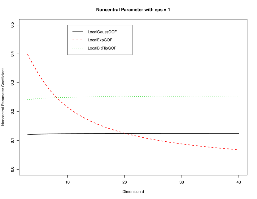
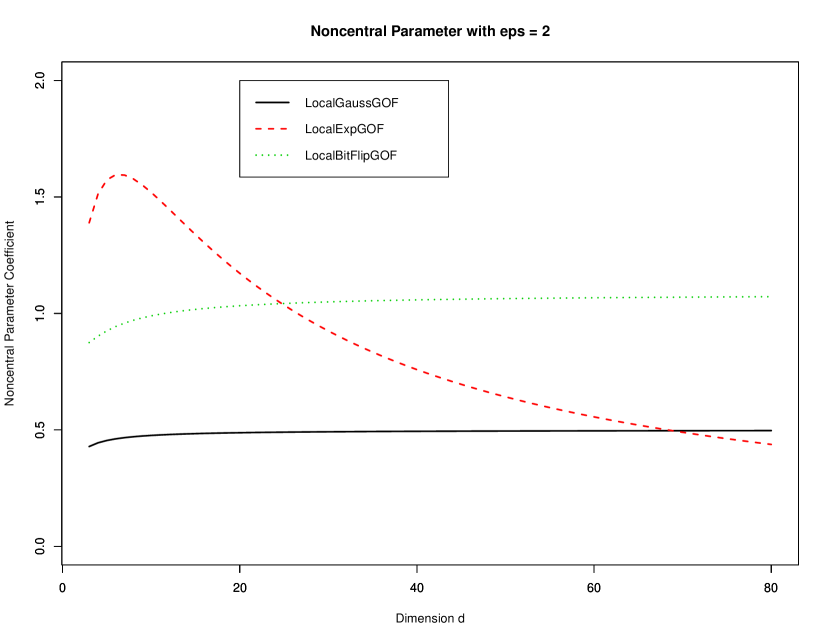
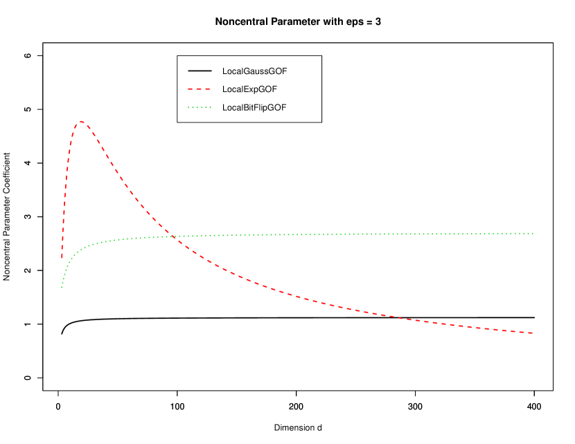
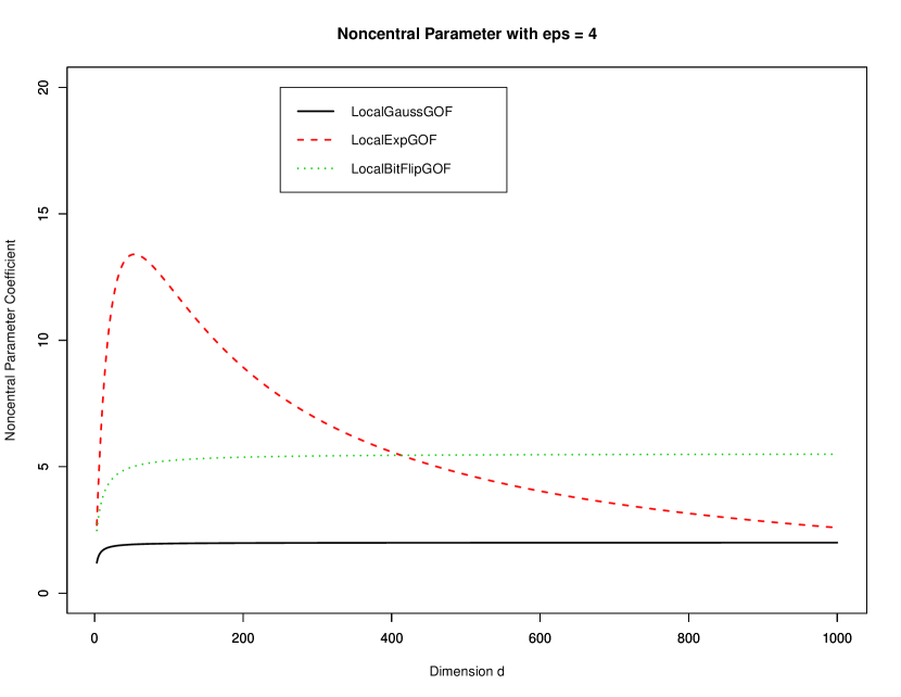
Figure 1: The coefficient on $\boldsymbol{\Delta}^{\intercal}\boldsymbol{\Delta}$ in the noncentral parameter for the local private tests where “LocalGaussGOF" is LocalNoiseGOF with Gaussian noise, LocalExpGOF, and LocalBitFlipGOF for various dimensions $d$ and $\epsilon$.

5.4 Empirical Results

We then empirically compare the power between LocalNoiseGOF with Laplace noise in Algorithm 1, LocalExpGOF in Algorithm 3, and LocalBitFlipGOF in Algorithm 5. Recall that all three of these tests have the same privacy benchmark of local differential privacy. For LocalNoiseGOF with Laplace noise, we will use $m=999$ samples in out Monte Carlo simulations. In our experiments we fix $\alpha=0.05$ and $\epsilon\in\{1,2,4\}$. We then consider null hypotheses of the form $\boldsymbol{p}^{0}=(1/d,1/d,\cdots,1/d)$ and alternate $\mathrm{H}_{1}:\boldsymbol{p}=\boldsymbol{p}^{0}+\eta(1,-1,\cdots,1,-1)$ for some $\eta>0$. In Figure 2, we plot the number of times our tests correctly rejects the null hypothesis in 1000 independent trials for various sample sizes $n$ and privacy parameters $\epsilon$.

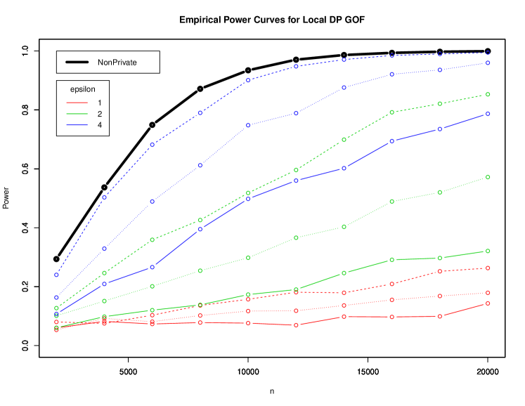
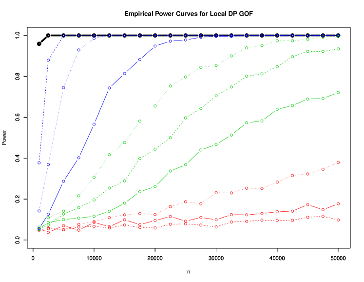
Figure 2: Comparison of empirical power among the classical non-private test and the local private tests LocalNoiseGOF with Laplace noise (solid line), LocalExpGOF (dashed line), and LocalBitFlipGOF (dotted line); in the left plot, $d=4$ and $\eta=0.01$, in the right plot, $d=40$ and $\eta=0.005$.

From Figure 2, we can see that the test statistics that have the largest noncentral parameter for a particular dimension $d$ and privacy parameter $\epsilon$ will have the best empirical power. When $d=4$, we see that LocalExpGOF performs the best. However, for $d=40$ it is not so clear cut. When $\epsilon=4$, we can see that LocalExpGOF does the best, but then when $\epsilon=2$, LocalBitFlipGOF does best. Thus, the best Local DP Goodness of Fit test depends on the noncentral parameter, which is a function of $\epsilon$, the null hypothesis $\boldsymbol{p}^{0}$, and alternate $\boldsymbol{p}=\boldsymbol{p}^{0}+\boldsymbol{\Delta}$. Note that the worst local DP test also depends on the privacy parameter and the dimension $d$. Based on our empirical results, we see that no single locally private test is best for all data dimensions. Knowing the corresponding noncentral parameter for a given problem is useful in determining which tests to use, where the larger the noncentral parameter is the higher the power will be.

6 Local Private Independence Tests

We now show that our techniques can be extended to include composite hypothesis tests, where we test whether the data comes from a whole family of probability distributions. We will focus on independence testing, but much of the theory can be extended to general chi-square tests. We will closely follow the presentation and notation as in (Kifer and Rogers, 2017).

We consider two multinomial random variables $\{\boldsymbol{U}_{\ell}\}^{n}_{\ell=1}\stackrel{{\scriptstyle i.i.d.}}{{\sim}}\mathrm{Multinomial}(1,\boldsymbol{\pi}^{(1)})$ for $\boldsymbol{\pi}^{(1)}\in\mathbb{R}^{r}$, $\{\boldsymbol{V}_{\ell}\}_{\ell=1}^{n}\stackrel{{\scriptstyle i.i.d.}}{{\sim}}\mathrm{Multinomial}(1,\boldsymbol{\pi}^{(2)})$ for $\boldsymbol{\pi}^{(2)}\in\mathbb{R}^{c}$ and no component of $\boldsymbol{\pi}^{(1)}$ or $\boldsymbol{\pi}^{(2)}$ is zero. Without loss of generality, we will consider an individual to be in one of $r$ groups who reports a data record that is in one of $c$ categories. The collected data consists of $n$ joint outcomes $\boldsymbol{H}$ whose $(i,j)$th coordinate is $H_{i,j}=\sum_{\ell=1}^{n}\mathbbm{1}\{U_{\ell,i}=1\quad\&\quad V_{\ell,j}=1\}$. Note that $\boldsymbol{H}$ is then the contingency table over the joint outcomes.

Under the null hypothesis of independence between $\{\boldsymbol{U}_{\ell}\}^{n}_{\ell=1}$ and $\{\boldsymbol{V}_{\ell}\}^{n}_{\ell=1}$, we have

$$\boldsymbol{H}\sim\mathrm{Multinomial}\left(n,\boldsymbol{p}(\boldsymbol{\pi}^{(1)},\boldsymbol{\pi}^{(2)})\right)\qquad\text{ where }\boldsymbol{p}(\boldsymbol{\pi}^{(1)},\boldsymbol{\pi}^{(2)})=\boldsymbol{\pi}^{(1)}\left(\boldsymbol{\pi}^{(2)}\right)^{\intercal}$$ (8)

What makes this test difficult is that the analyst does not know the data distribution $\boldsymbol{p}(\boldsymbol{\pi}^{(1)},\boldsymbol{\pi}^{(2)})$ and so cannot simply plug it into the chi-square statistic. Rather, we use the data to estimate the best guess for the unknown probability distribution that satisfies the null hypothesis.

Note that without privacy, each individual $\ell\in[n]$ is reporting a $r\times c$ matrix $\boldsymbol{X}_{\ell}$ which would be 1 in exactly one location. Thus we can alternatively write the contingency table as $\boldsymbol{H}=\sum_{\ell=1}^{n}\boldsymbol{X}_{\ell}$. We then use the three local private algorithms we presented earlier for noise addition, exponential mechanism, and bit flipping to see how we can form a private chi-square statistic for independence testing. We want to be able to ensure the privacy of both the group and the category that each individual belongs to.

For completeness, we will present the minimum chi-square asymptotic theory from Ferguson (1996) that was used in Kifer and Rogers (2017). We will use this theory to design general chi-square test statistics for local differentially private hypothesis tests. Consider a $d$ dimensional random vector $\boldsymbol{V}^{(n)}$ and a $k\leq d$ dimensional parameter space $\Theta$, which is an open subset of $\mathbb{R}^{k}$. We want to measure the distance between the random variable $\boldsymbol{V}^{(n)}$ and some model $A(\boldsymbol{\theta})$ that maps parameters in $\Theta$ to $\mathbb{R}^{d}$. We then use the following quadratic form where $M(\boldsymbol{\theta})\in\mathbb{R}^{d\times d}$ is a positive-semidefinite matrix.

$$n\left(\boldsymbol{V}^{(n)}-A(\boldsymbol{\theta})\right)^{\intercal}M(\boldsymbol{\theta})\left(\boldsymbol{V}^{(n)}-A(\boldsymbol{\theta})\right)$$ (9)

We want to ensure the following assumptions hold.

Assumption 6.1.

For all $\boldsymbol{\theta}\in\Theta$, we have

• There exists a parameter $\boldsymbol{\theta}^{\star}\in\Theta$ such that for some model $A(\cdot)$ and covariance matrix $C(\cdot)$

  $$\sqrt{n}\left(\boldsymbol{V}^{(n)}-A(\boldsymbol{\theta}^{\star})\right)\stackrel{{\scriptstyle D}}{{\to}}\mathrm{N}\left(\boldsymbol{0},C(\boldsymbol{\theta}^{\star})\right)$$

• $A(\boldsymbol{\theta})$ is bicontinuous.

• $A(\boldsymbol{\theta})$ has continuous first partial derivatives, denoted as $\dot{A}(\boldsymbol{\theta})$, with full rank $k$.

• The matrix $M(\boldsymbol{\theta})$ is continuous in $\boldsymbol{\theta}$ and there exists an $\eta>0$ such that $M(\boldsymbol{\theta})-\eta I_{d}$ is positive definite in an open neighborhood of $\boldsymbol{\theta}^{\star}$.

We will then use the following useful result from Kifer and Rogers (2017)[Theorem 4.2].

Theorem 6.2 (Kifer and Rogers (2017)).

Let $\nu$ be the rank of $C(\boldsymbol{\theta}^{\star})$. If 6.1 holds, and for all $\boldsymbol{\theta}\in\Theta$ we have

$$C(\boldsymbol{\theta})M(\boldsymbol{\theta})C(\boldsymbol{\theta})=C(\boldsymbol{\theta})$$

$$C(\boldsymbol{\theta})M(\boldsymbol{\theta})\dot{A}(\boldsymbol{\theta})=\dot{A}(\boldsymbol{\theta})$$

Then for any estimate $\phi(\boldsymbol{V}^{(n)})\stackrel{{\scriptstyle P}}{{\to}}\boldsymbol{\theta}^{\star}$ we have

$$\min_{\boldsymbol{\theta}\in\Theta}\left\{n\left(\boldsymbol{V}^{(n)}-A(\boldsymbol{\theta})\right)^{\intercal}M(\phi(\boldsymbol{V}^{(n)}))\left(\boldsymbol{V}^{(n)}-A(\boldsymbol{\theta})\right)\right\}\stackrel{{\scriptstyle D}}{{\to}}\chi^{2}_{\nu-k}.$$

To ensure the assumptions hold, we will assume that each component of $\boldsymbol{\pi}^{(1)},\boldsymbol{\pi}^{(2)}$ is positive, i.e. $\boldsymbol{\pi}^{(i)}>0$ for $i=1,2$.

6.1 Independence Test with Noise Addition

For noise addition, we will have the following contingency table $\boldsymbol{H}+\boldsymbol{Z}$ (treating $\boldsymbol{H}$ as an $r\times c$ vector) where $\boldsymbol{Z}=\mathrm{N}\left(\boldsymbol{0},\frac{n}{\rho}\right)$ for $\rho$-LzCDP or $\boldsymbol{Z}$ is the sum of $n$ independent Laplace random vectors with scale parameter $2/\epsilon$ in each coordinate for $\epsilon$-LDP, although we will only consider the Gaussian noise case. We can then use the same statistic presented in Kifer and Rogers (2017) with a rescaling of the variance in the noise and flattening the contingency table as a vector. For convenience, we write the marginals as $H_{i,\cdot}=\sum_{j=1}^{c}H_{i,j}$ and similarly for $H_{\cdot,j}$. Further, we will write $\widehat{n}=n+\sum_{i,j}Z_{i,j}$ in the following test statistic,

$$\widehat{\boldsymbol{\pi}}^{(1)} =\left(\frac{1}{\widehat{n}}\left(H_{i,\cdot}+Z_{i,\cdot}\right):i\in[r]\right),\qquad\widehat{\boldsymbol{\pi}}^{(2)}=\left(\frac{1}{\widehat{n}}\left(H_{\cdot,j}+Z_{\cdot,j}\right):j\in[c]\right)$$

$$\widehat{M} =\mathrm{Diag}\left(\boldsymbol{p}(\widehat{\boldsymbol{\pi}}^{(1)},\widehat{\boldsymbol{\pi}}^{(2)})\right)-\boldsymbol{p}(\widehat{\boldsymbol{\pi}}^{(1)},\widehat{\boldsymbol{\pi}}^{(2)})\left(\boldsymbol{p}(\widehat{\boldsymbol{\pi}}^{(1)},\widehat{\boldsymbol{\pi}}^{(2)})\right)^{\intercal}+\frac{1}{\rho}I_{rc}$$

$$\boldsymbol{\widehat{\mathrm{T}}}^{(n)}_{KR}\left(\rho/n;(\boldsymbol{\pi}^{(1)},\boldsymbol{\pi}^{(2)})\right) =\frac{1}{n}\left(\boldsymbol{H}+\boldsymbol{Z}-n\boldsymbol{p}\left(\boldsymbol{\pi}^{(1)},\boldsymbol{\pi}^{(2)}\right)\right)^{\intercal}\Pi\left(\widehat{M}\right)^{-1}\Pi\left(\boldsymbol{H}+\boldsymbol{Z}-n\boldsymbol{p}\left(\boldsymbol{\pi}^{(1)},\boldsymbol{\pi}^{(2)}\right)\right)$$ (10)

We use this statistic because it is asymptotically distributed as a chi-square random variable given the null hypothesis holds, which follows directly from the general chi-square theory presented in Kifer and Rogers (2017).

Theorem 6.3.

Under the null hypothesis that $\boldsymbol{U}$ and $\boldsymbol{V}$ are independent, then we have as $n\to\infty$

$$\min_{\boldsymbol{\pi}^{(1)},\boldsymbol{\pi}^{(2)}}\left\{\boldsymbol{\widehat{\mathrm{T}}}^{(n)}_{KR}\left(\rho/n;(\boldsymbol{\pi}^{(1)},\boldsymbol{\pi}^{(2)})\right)\right\}\stackrel{{\scriptstyle D}}{{\to}}\chi^{2}_{(r-1)(c-1)}.$$

We present the test in Algorithm 6 for Gaussian noise which uses the statistic in (10).

Algorithm 6 LzCDP Independence Test with Gaussian Mechanism: LocalNoiseIND

0:  $(\boldsymbol{x}_{1},\cdots,\boldsymbol{x}_{n})$, $\rho$, $\alpha$.

  Let $\boldsymbol{H}=\sum_{\ell=1}^{n}\boldsymbol{x}_{\ell}$

  Set $q=\min_{\boldsymbol{\pi}^{(1)},\boldsymbol{\pi}^{(2)}}\left\{\boldsymbol{\widehat{\mathrm{T}}}^{(n)}_{KR}\left(\rho/n;(\boldsymbol{\pi}^{(1)},\boldsymbol{\pi}^{(2)})\right)\right\}$ given in (10).

  if $q>\chi_{(r-1)(c-1),1-\alpha}^{2}$ then

     Decision $\leftarrow$ Reject.

  else

     Decision $\leftarrow$ Fail to Reject.

  Decision

We then have the following result which follows from the privacy analysis from before.

Theorem 6.4.

LocalNoiseIND is $\rho$-LzCDP.

6.2 Independence Test with the Exponential Mechanism

Next we want to design an independence test when the data is generated from $\mathcal{M}_{\mathtt{EXP}}$ given in Algorithm 2. In this case our contingency table can be written as $\check{\boldsymbol{H}}\sim\mathrm{Multinomial}\left(n,\check{\boldsymbol{p}}(\boldsymbol{\pi}^{(1)},\boldsymbol{\pi}^{(2)})\right)$ where $\beta_{\epsilon}=\frac{1}{e^{\epsilon}+rc-1}$ and we use (4) to get

$$\check{\boldsymbol{p}}(\boldsymbol{\pi}^{(1)},\boldsymbol{\pi}^{(2)})=\beta_{\epsilon}\left(\left(e^{\epsilon}-1\right)\boldsymbol{\pi}^{(1)}\left(\boldsymbol{\pi}^{(2)}\right)^{\intercal}\ +\boldsymbol{1}\right)$$ (11)

We then obtain an estimate for the unknown parameters,

$$\check{\boldsymbol{\pi}}^{(1)} =\frac{1}{\beta_{\epsilon}\left(e^{\epsilon}-1\right)}\left(\frac{\check{H}_{i,\cdot}}{n}-c\beta_{\epsilon}:i\in[r]\right),$$

$$\check{\boldsymbol{\pi}}^{(2)} =\frac{1}{\beta_{\epsilon}\left(e^{\epsilon}-1\right)}\left(\frac{\check{H}_{\cdot,j}}{n}-r\beta_{\epsilon}:j\in[c]\right)$$

$$\check{\boldsymbol{\mathrm{T}}}_{\mathrm{Exp}}^{(n)}\left(\epsilon\right) =\sum_{i,j}\frac{\left(\check{H}_{i,j}-n\check{p}_{i,j}\left(\check{\boldsymbol{\pi}}^{(1)},\check{\boldsymbol{\pi}}^{(2)}\right)\right)^{2}}{n\check{p}_{i,j}(\check{\boldsymbol{\pi}}^{(1)},\check{\boldsymbol{\pi}}^{(2)})}$$ (12)

We can then prove the following result, which uses Theorem 6.2.

Theorem 6.5.

Assuming $\boldsymbol{U}$ and $\boldsymbol{V}$ are independent with true probability vectors $\boldsymbol{\pi}^{(1)},\boldsymbol{\pi}^{(2)}>0$ respectively, then as $n\to\infty$ we have $\check{\boldsymbol{\mathrm{T}}}_{\mathrm{Exp}}^{(n)}\left(\epsilon\right)\stackrel{{\scriptstyle D}}{{\to}}\chi^{2}_{(r-1)(c-1)}$.

Proof.

Note that $\check{\boldsymbol{\pi}}^{(1)},\check{\boldsymbol{\pi}}^{(2)}$ both converge in probability to the true parameters $\boldsymbol{\pi}^{(1)},\boldsymbol{\pi}^{(2)}$, respectively due to $\mathbb{E}\left[\check{\boldsymbol{H}}/n\right]=\check{\boldsymbol{p}}(\boldsymbol{\pi}^{(1)},\boldsymbol{\pi}^{(2)})$ and $\mathbb{V}\left[\check{\boldsymbol{H}}/n\right]\to 0$. We then form the following statistic in terms of parameters $\boldsymbol{\theta}^{(1)}$ in the $r$ dimensional simplex with all positive components and $\boldsymbol{\theta}^{(2)}$ in the $c$ dimensional simplex with all positive components,

$$\check{\boldsymbol{\mathrm{T}}}_{\mathrm{Exp}}^{(n)}\left(\boldsymbol{\theta}^{(1)},\boldsymbol{\theta}^{(2)};\epsilon\right)$$

$$\quad=n\left(\check{\boldsymbol{H}}/n-\check{\boldsymbol{p}}(\boldsymbol{\theta}^{(1)},\boldsymbol{\theta}^{(2)})\right)^{\intercal}\mathrm{Diag}\left(\check{\boldsymbol{p}}(\check{\boldsymbol{\pi}}^{(1)},\check{\boldsymbol{\pi}}^{(2)})\right)^{-1}\left(\check{\boldsymbol{H}}/n-\check{\boldsymbol{p}}(\boldsymbol{\theta}^{(1)},\boldsymbol{\theta}^{(2)})\right)$$

We then have the following calculation,

$$\left(\check{\boldsymbol{\pi}}^{(1)},\check{\boldsymbol{\pi}}^{(2)}\right)=\operatorname*{\arg\!\min}_{\boldsymbol{\theta}^{(1)},\boldsymbol{\theta}^{(2)}}\left\{\check{\boldsymbol{\mathrm{T}}}_{\mathrm{Exp}}^{(n)}\left(\boldsymbol{\theta}^{(1)},\boldsymbol{\theta}^{(2)};\epsilon\right)\right\}.$$

Note that $\sqrt{n}\left(\check{\boldsymbol{H}}/n-\check{\boldsymbol{p}}(\boldsymbol{\pi}^{(1)},\boldsymbol{\pi}^{(2)})\right)\stackrel{{\scriptstyle D}}{{\to}}\mathrm{N}\left(\boldsymbol{0},C(\boldsymbol{\theta})\right)$ where $C(\boldsymbol{\theta})=\mathrm{Diag}(\check{\boldsymbol{p}}(\boldsymbol{\theta}^{(1)},\boldsymbol{\theta}^{(2)}))-\check{\boldsymbol{p}}(\boldsymbol{\theta}^{(1)},\boldsymbol{\theta}^{(2)})\left(\check{\boldsymbol{p}}(\boldsymbol{\theta}^{(1)},\boldsymbol{\theta}^{(2)})\right)^{\intercal}$ is the covariance matrix for the multinomial random variable.

We then apply Theorem 6.2 to prove the statement, so we verify that the following equalities hold,

$$C(\boldsymbol{\theta})\cdot\mathrm{Diag}\left(\check{\boldsymbol{p}}(\boldsymbol{\theta}^{(1)},\boldsymbol{\theta}^{(2)})\right)^{-1}\cdot C(\boldsymbol{\theta})=C(\boldsymbol{\theta})$$

and

$$C(\boldsymbol{\theta}) \cdot\mathrm{Diag}\left(\check{\boldsymbol{p}}(\boldsymbol{\theta}^{(1)},\boldsymbol{\theta}^{(2)})\right)^{-1}\nabla\left(\boldsymbol{\theta}^{(1)}\left(\boldsymbol{\theta}^{(2)}\right)^{\intercal}\right)$$

$$=\left(I_{rc}-\check{\boldsymbol{p}}(\boldsymbol{\theta}^{(1)},\boldsymbol{\theta}^{(2)})\boldsymbol{1}^{\intercal}\right)\nabla\left(\boldsymbol{\theta}^{(1)}\left(\boldsymbol{\theta}^{(2)}\right)^{\intercal}\right)$$

$$=\nabla\left(\boldsymbol{\theta}^{(1)}\left(\boldsymbol{\theta}^{(2)}\right)^{\intercal}\right)$$

where the last equality follows from the last coordinates of each probability vector can be written as $\theta^{(1)}_{r}=1-\sum_{i=1}^{r-1}\theta_{i}$ and $\theta^{(2)}_{c}=1-\sum_{j=1}^{c-1}\theta_{j}^{(2)}$. ∎

We then use this result to design our private chi-square test for independence.

Algorithm 7 Local DP IND Test: LocalExpIND

0:  $\boldsymbol{x}=(\boldsymbol{x}_{1},\cdots,\boldsymbol{x}_{n})$, $\epsilon$, $\alpha$, $\mathrm{H}_{0}:\boldsymbol{p}=\boldsymbol{p}^{0}$.

  Let $\check{\boldsymbol{H}}=\sum_{i=1}^{n}\mathcal{M}_{\mathtt{EXP}}(\boldsymbol{x}_{i},\epsilon)$.

  Set $q=\check{\boldsymbol{\mathrm{T}}}_{\mathrm{Exp}}^{(n)}\left(\epsilon\right)$ from (12)

  if $q>\chi_{d-1,1-\alpha}^{2},$ Decision $\leftarrow$ Reject.

  else Decision $\leftarrow$ Fail to Reject.

  Decision

We then have the following result which again follows from the privacy analysis from before.

Theorem 6.6.

LocalExpIND is $\epsilon$-LDP.

6.3 Independence Test with Bit Flipping

Lastly, we design an independence test when the data is reported via $\mathcal{M}_{\text{bit}}$ in Algorithm 4. Assuming that $\boldsymbol{H}=\sum_{\ell=1}^{n}\boldsymbol{X}_{\ell}\sim\mathrm{Multinomial}\left(n,\boldsymbol{p}(\boldsymbol{\pi}^{(1)},\boldsymbol{\pi}^{(2)})\right)$, then we know that replacing $\boldsymbol{p}^{0}$ with $\boldsymbol{p}(\boldsymbol{\pi}^{(1)},\boldsymbol{\pi}^{(2)})$ in Section 5.2 gives us the following asymptotic distribution (treating the contingency table of values as a vector) with covariance matrix $\Sigma(\cdot)$ given in (6)

$$\sqrt{n}\left(\frac{\widetilde{\boldsymbol{H}}}{n}-\left[\underbrace{\left(\frac{e^{\epsilon/2}-1}{e^{\epsilon/2}+1}\right)\boldsymbol{\pi}^{(1)}\left(\boldsymbol{\pi}^{(2)}\right)^{\intercal}+\frac{1}{e^{\epsilon/2}+1}}_{\widetilde{\boldsymbol{p}}(\boldsymbol{\pi}^{(1)},\boldsymbol{\pi}^{(2)})}\right]\right)$$

$$\qquad\stackrel{{\scriptstyle D}}{{\to}}\mathrm{N}\left(\boldsymbol{0},\Sigma\left(\boldsymbol{\pi}^{(1)}\left(\boldsymbol{\pi}^{(2)}\right)^{\intercal}\right)\right)$$ (13)

Similar to analysis for Theorem 6.5, we start with a rough estimate for the unknown parameters which converges in probability to the true estimates, so we again use $\alpha_{\epsilon}=\left(\frac{e^{\epsilon/2}-1}{e^{\epsilon/2}+1}\right)$ to get

$$\widetilde{\boldsymbol{\pi}}^{(1)} =\left(\frac{1}{\alpha_{\epsilon}}\right)\left(\frac{\widetilde{H}_{i,\cdot}}{n}-\frac{c}{e^{\epsilon/2}+1}:i\in[r]\right)$$

$$\widetilde{\boldsymbol{\pi}}^{(2)} =\left(\frac{1}{\alpha_{\epsilon}}\right)\left(\frac{\widetilde{H}_{\cdot,j}}{n}-\frac{r}{e^{\epsilon/2}+1}:j\in[c]\right)$$ (14)

We then give the resulting statistic, parameterized by the unknown parameters $\boldsymbol{\pi}^{(\ell)}$, for $\ell\in\{1,2\}$. For middle matrix $\widetilde{M}=\Pi\Sigma\left(\widetilde{\boldsymbol{\pi}}^{(1)}\left(\widetilde{\boldsymbol{\pi}}^{(2)}\right)^{\intercal}\right)^{-1}\Pi$, we have

$$\widetilde{\boldsymbol{\mathrm{T}}}_{\text{BitFlip}}^{(n)}\left(\boldsymbol{\theta}^{(1)},\boldsymbol{\theta}^{(2)};\epsilon\right)=\frac{1}{n}\left(\widetilde{\boldsymbol{H}}-n\widetilde{\boldsymbol{p}}\left(\boldsymbol{\theta}^{(1)},\boldsymbol{\theta}^{(2)}\right)\right)^{\intercal}$$

$$\qquad\widetilde{M}\left(\widetilde{\boldsymbol{H}}-n\widetilde{\boldsymbol{p}}\left(\boldsymbol{\theta}^{(1)},\boldsymbol{\theta}^{(2)}\right)\right)$$ (15)

Theorem 6.7.

Under the null hypothesis that $\boldsymbol{U}$ and $\boldsymbol{V}$ are independent with true probability vectors $\boldsymbol{\pi}^{(1)},\boldsymbol{\pi}^{(2)}>0$ respectively, then we have as $n\to\infty$, $\min_{\boldsymbol{\theta}^{(1)},\boldsymbol{\theta}^{(2)}}\left\{\widetilde{\boldsymbol{\mathrm{T}}}_{\text{BitFlip}}^{(n)}\left(\boldsymbol{\theta}^{(1)},\boldsymbol{\theta}^{(2)};\epsilon\right)\right\}\stackrel{{\scriptstyle D}}{{\to}}\chi^{2}_{(r-1)(c-1)}.$

Proof.

As in the proof of Theorem 6.5, we will use Theorem 6.2, so we first need to the verify the following equality holds, where $\boldsymbol{p}(\boldsymbol{\theta})=\boldsymbol{\theta}^{(1)}\left(\boldsymbol{\theta}^{(2)}\right)^{\intercal}$

$$\Pi\Sigma\left(\boldsymbol{p}(\boldsymbol{\theta})\right)\Pi\cdot\Sigma\left(\boldsymbol{p}(\boldsymbol{\theta})\right)^{-1}\cdot\Pi\Sigma\left(\boldsymbol{p}(\boldsymbol{\theta})\right)\Pi=\Pi\Sigma\left(\boldsymbol{p}(\boldsymbol{\theta})\right)\Pi.$$

Recall that $\Sigma(\boldsymbol{p}(\boldsymbol{\theta}))$ has an eigenvector of all 1’s and the other eigenvectors are orthogonal to it. Hence, when we diagonalize $\Sigma(\boldsymbol{p}(\boldsymbol{\theta}))=BDB^{\intercal}$, then $\Pi B$ is going to be the same as $B$ except the column of all 1’s becomes zero, which we will denote as $B^{*}$. Hence, $\Sigma(\boldsymbol{p}(\boldsymbol{\theta}))\Pi\Sigma(\boldsymbol{p}(\boldsymbol{\theta}))^{-1}\Pi\Sigma(\boldsymbol{p}(\boldsymbol{\theta}))$, becomes $BD^{*}B^{\intercal}$ where $D^{*}$ is the same as $D$ except the eigenvalue on the diagonal for the eigenvector of all 1’s becomes zero. Then projecting the resulting matrix with $\Pi$ will not change the resulting product We then have

$$\Pi\Sigma\left(\boldsymbol{p}(\boldsymbol{\theta})\right)\Pi\cdot\Sigma\left(\boldsymbol{p}(\boldsymbol{\theta})\right)^{-1}\cdot\Pi\Sigma\left(\boldsymbol{p}(\boldsymbol{\theta})\right)\Pi$$

$$\qquad=\Pi BD^{*}B^{\intercal}\Pi=\Pi\Sigma(\boldsymbol{p}(\boldsymbol{\theta}))\Pi.$$

We then need to show that the following equality holds

$$\Pi\Sigma\left(\boldsymbol{p}(\boldsymbol{\theta})\right)\Pi\cdot\Sigma(\boldsymbol{p}(\boldsymbol{\theta}))^{-1}\Pi\nabla\widetilde{\boldsymbol{p}}(\boldsymbol{\theta}^{(1)},\boldsymbol{\theta}^{(2)})$$

$$\qquad=\Pi\nabla\widetilde{\boldsymbol{p}}(\boldsymbol{\theta}^{(1)},\boldsymbol{\theta}^{(2)})$$

We again use the fact that $\Sigma(\boldsymbol{p}(\boldsymbol{\theta}))$ has an eigenvector that is all 1’s. Hence, we have

$$\Pi\Sigma(\boldsymbol{p}(\boldsymbol{\theta}))\Pi=\Sigma(\boldsymbol{p}(\boldsymbol{\theta}))-\frac{e^{\epsilon/2}}{rc\cdot(e^{\epsilon/2}+1)^{2}}\boldsymbol{1}\boldsymbol{1}^{\intercal}.$$

We then have,

$$\Pi\Sigma\left(\boldsymbol{p}(\boldsymbol{\theta})\right)\Pi\cdot\Sigma(\boldsymbol{p}(\boldsymbol{\theta}))^{-1}\Pi\nabla\widetilde{\boldsymbol{p}}(\boldsymbol{\theta}^{(1)},\boldsymbol{\theta}^{(2)})$$

$$\quad=\left(\Sigma(\boldsymbol{p}(\boldsymbol{\theta}))-\frac{e^{\epsilon/2}}{rc\cdot(e^{\epsilon/2}+1)^{2}}\boldsymbol{1}\boldsymbol{1}^{\intercal}\right)$$

$$\qquad\qquad\cdot\Sigma(\boldsymbol{p}(\boldsymbol{\theta}))^{-1}\Pi\nabla\widetilde{\boldsymbol{p}}(\boldsymbol{\theta}^{(1)},\boldsymbol{\theta}^{(2)})$$

$$\quad=\left(I_{rc}-\frac{1}{rc}\boldsymbol{1}\boldsymbol{1}^{\intercal}\right)\Pi\nabla\widetilde{\boldsymbol{p}}(\boldsymbol{\theta}^{(1)},\boldsymbol{\theta}^{(2)})$$

$$\quad=\Pi\Pi\nabla\widetilde{\boldsymbol{p}}(\boldsymbol{\theta}^{(1)},\boldsymbol{\theta}^{(2)})=\Pi\nabla\widetilde{\boldsymbol{p}}(\boldsymbol{\theta}^{(1)},\boldsymbol{\theta}^{(2)}).$$

∎

Algorithm 8 Local DP IND Test: LocalBitFlipIND

0:  $(\boldsymbol{x}_{1},\cdots,\boldsymbol{x}_{n})$, $\epsilon$, $\alpha$.

  Let $\widetilde{\boldsymbol{H}}=\sum_{i=1}^{n}\mathcal{M}_{\text{bit}}(\boldsymbol{x}_{i},\epsilon)$.

  $q=\min_{\boldsymbol{\pi}^{(1)},\boldsymbol{\pi}^{(2)}}\left\{\widetilde{\boldsymbol{\mathrm{T}}}_{\text{BitFlip}}^{(n)}\left(\epsilon;(\boldsymbol{\pi}^{(1)},\boldsymbol{\pi}^{(2)})\right)\right\}$ from (15).

  if $q>\chi_{(r-1)(c-1),1-\alpha}^{2}$ Decision $\leftarrow$ Reject.

  else Decision $\leftarrow$ Fail to Reject.

  Decision

We present the test in Algorithm 8. The following result follows from same privacy analysis as before.

Theorem 6.8.

LocalBitFlipIND is $\epsilon$-LDP.

6.4 Empirical Results

As we did for the locally private goodness of fit tests, we empirically compare the power for our various tests for independence. We consider the null hypothesis that the two sequences of categorical random variables $\{\boldsymbol{U}_{\ell}\}_{\ell=1}^{n}$ and $\{\boldsymbol{V}_{\ell}\}_{\ell=1}^{n}$ are independent of one another. Under an alternate hypothesis, we generate the contingency data according to a non-product distribution. We fix the distribution $\boldsymbol{p}^{(1)}$ for the contingency table to be of the following form, where $\boldsymbol{\pi}^{(1)}\in\mathbb{R}^{r}$ is the unknown distribution for $\{\boldsymbol{U}_{\ell}\}_{\ell=1}^{n}$, $\boldsymbol{\pi}^{(2)}\in\mathbb{R}^{c}$ is the unknown distribution for $\{\boldsymbol{V}_{\ell}\}_{\ell=1}^{n}$, and $r,c$ are even

$$\boldsymbol{p}^{(1)}=\boldsymbol{\pi}^{(1)}\left(\boldsymbol{\pi}^{(2)}\right)^{\intercal}$$

$$\quad+\eta(1,-1,\cdots,-1,1)^{\intercal}(1,-1,\cdots,-1,1)$$ (16)

Note that the hypothesis test does not know the underlying $\boldsymbol{\pi}^{(i)}$ for $i\in\{1,2\}$, but to generate the data we must fix these distributions. We show power results when the marginal distributions satisfy $\boldsymbol{\pi}^{(1)}=(1/r,\cdots,1/r)$ and $\boldsymbol{\pi}^{(2)}=(1/c,\cdots,1/c)$. In Figure 3, we give results for various $n$ and $\epsilon\in\{1,2,4\}$ for the case when $(r,c)=(2,2)$ and $\eta=0.01$ as well as the case when $(r,c)=(10,4)$ and $\eta=0.005$.

Note that we only give results for the two tests LocalExpIND and LocalBitFlipIND.

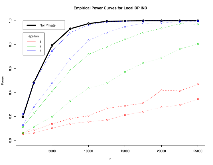
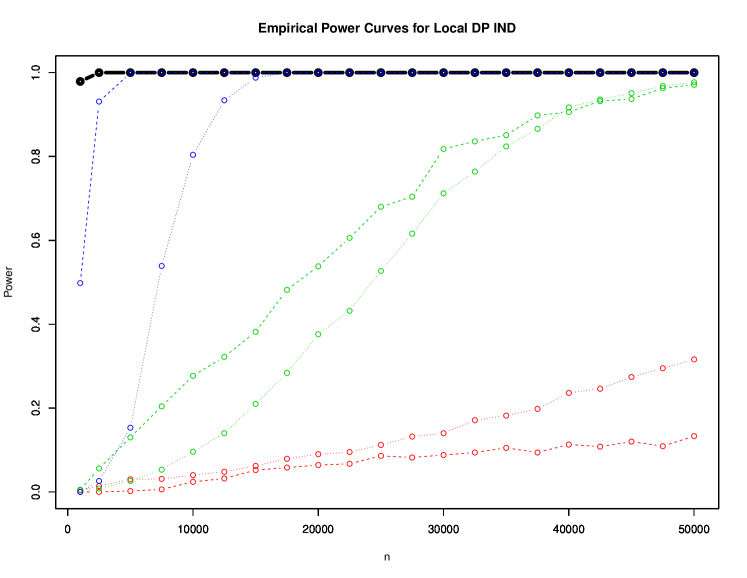
Figure 3: Comparison of empirical power of classical non-private test versus local private tests LocalExpIND (dashed line), and LocalBitFlipIND (dotted line). In the left plot we set $(r,c)=(2,2)$ and $\eta=0.01$ while we set $(r,c)=(10,4)$ and $\eta=0.005$ in the right plot for the contingency table data distribution given in (16).

7 Conclusion

We have designed several hypothesis tests, each depending on different local differentially private algorithms: LocalNoiseGOF (LocalLapGOF), LocalExpGOF, and LocalBitFlipGOF as well as their corresponding independence tests LocalNoiseIND, LocalExpIND, and LocalBitFlipIND. This required constructing different statistics so that the resulting distribution after injecting noise into the data in order to satisfy privacy could be closely approximated with a chi-square distribution. Hence, we designed rules for when a null hypothesis $\mathrm{H}_{0}$ should be rejected while satisfying some bound $\alpha$ on Type I error. Further, We showed that each statistic has a noncentral chi-square distribution when the data is drawn from some alternate hypothesis $\mathrm{H}_{1}$. Depending on the form of the alternate probability distribution, the dimension of the data, and the privacy parameter, either LocalExpGOF or LocalBitFlipGOF gave better power. This corroborates the results from Kairouz et al. (2014) who showed that in hypothesis testing, different privacy regimes have different optimal local differentially private mechanisms, although utility in their work was in terms of KL divergence. Our results show that the power of the test is directly related to the noncentral parameter of the test statistic that is used. This requires the data analyst to carefully consider alternate hypotheses, as well as the data dimension and privacy parameter for a particular test and then see which test statistic results in the largest noncentral parameter. We focused primarily on goodness of fit testing, where the null hypothesis is a single probability distribution. We further developed local private independence tests which resulted in using previous general chi-square theory presented in Kifer and Rogers (2017). This basic framework can be used to develop other chi-square hypothesis tests where the null hypothesis is not a single parameter. We hope that this will lead to future work on designing local differentially private hypothesis tests beyond chi-square testing.

Appendix A Omitted Proofs

Proof of Lemma 5.7.

This follows from the central limit theorem. We first compute the expected value

$$\frac{1}{n}\mathbb{E}\left[\widetilde{\boldsymbol{H}}\right]=\frac{e^{\epsilon/2}}{e^{\epsilon/2}+1}\boldsymbol{p}+\frac{1}{e^{\epsilon/2}+1}(1-\boldsymbol{p}).$$

In order to compute the covariance matrix, we consider the diagonal term $(j,j)$

$$\mathbb{E}\left[(\widetilde{H}_{j})^{2}\right]=\frac{e^{\epsilon/2}}{e^{\epsilon/2}+1}p_{j}+\frac{1}{e^{\epsilon/2}+1}(1-p_{j})$$

Next we compute the off diagonal term $(j,k)$

$$\mathbb{E}\left[\widetilde{H}_{j}\ \widetilde{H}_{k}\right] =\left(\frac{e^{\epsilon/2}}{e^{\epsilon/2}+1}\right)^{2}\mathrm{Pr}\left[X_{j}=1\ \&\ X_{k}=1\right]$$

$$\qquad+\frac{e^{\epsilon/2}}{\left(e^{\epsilon/2}+1\right)^{2}}\left(\mathrm{Pr}\left[X_{j}=1\ \&\ X_{k}=0\right]+\mathrm{Pr}\left[X_{j}=0\ \&\ X_{k}=1\right]\right)$$

$$\qquad+\frac{1}{\left(e^{\epsilon/2}+1\right)^{2}}\mathrm{Pr}\left[X_{j}=0\ \&\ X_{k}=0\right]$$

$$=\left(\frac{1}{e^{\epsilon/2}+1}\right)^{2}\left[e^{\epsilon/2}\left(p_{j}+p_{k}\right)+(1-p_{j}-p_{k})\right]$$

Before we construct the covariance matrix, we simplify a few terms

$$\mathbb{E}\left[(\widetilde{H}_{j})^{2}\right]-\mathbb{E}\left[\widetilde{H}_{j}\right]^{2}$$

$$\qquad=\left(\frac{1}{e^{\epsilon/2}+1}\right)^{2}\left[\left(e^{\epsilon/2}-1\right)\left(e^{\epsilon/2}+1\right)p_{j}+1+e^{\epsilon/2}-\left(\left(e^{\epsilon/2}-1\right)p_{j}+1\right)^{2}\right]$$

$$\qquad=\left(\frac{1}{e^{\epsilon/2}+1}\right)^{2}\left[\left(e^{\epsilon/2}-1\right)\left(e^{\epsilon/2}+1-2\right)p_{j}-(e^{\epsilon/2}-1)^{2}\left(p_{j}\right)^{2}+e^{\epsilon/2}\right]$$

$$\qquad=\frac{1}{\left(e^{\epsilon/2}+1\right)^{2}}\left[\left(e^{\epsilon/2}-1\right)^{2}p_{j}\left(1-p_{j}\right)+e^{\epsilon/2}\right]$$

Further, we have

$$\mathbb{E}\left[\widetilde{H}_{j}\widetilde{H}_{k}\right]-\mathbb{E}\left[\widetilde{H}_{j}\right]\mathbb{E}\left[\widetilde{H}_{k}\right]$$

$$\qquad=\left(\frac{1}{e^{\epsilon/2}+1}\right)^{2}\left[\left(e^{\epsilon/2}-1\right)\left(p_{j}+p_{k}\right)+1-\left((e^{\epsilon/2}-1)p_{j}+1\right)\left((e^{\epsilon/2}-1)p_{k}+1\right)\right]$$

$$\qquad=-\left(\frac{e^{\epsilon/2}-1}{e^{\epsilon/2}+1}\right)^{2}p_{j}p_{k}$$

Putting this together, the covariance matrix can then be written as

$$\Sigma(\boldsymbol{p}) =\mathbb{E}\left[\widetilde{\boldsymbol{H}}\left(\widetilde{\boldsymbol{H}}\right)^{\intercal}\right]-\mathbb{E}\left[\widetilde{\boldsymbol{H}}\right]\left(\mathbb{E}\left[\widetilde{\boldsymbol{H}}\right]\right)^{\intercal}$$

$$=\left(\frac{e^{\epsilon/2}-1}{e^{\epsilon/2}+1}\right)^{2}\left[\mathrm{Diag}\left(\boldsymbol{p}\right)-\boldsymbol{p}\left(\boldsymbol{p}\right)^{\intercal}\right]+\frac{e^{\epsilon/2}}{\left(e^{\epsilon/2}+1\right)^{2}}I_{d}$$

∎

References

• American Statistical Association [2014] American Statistical Association. Discovery with Data: Leveraging Statistics with Computer Science to Transform Science and Society, 2014. URL http://www.amstat.org/policy/pdfs/BigDataStatisticsJune2014.pdf.
• Apple Press Info [2016] Apple Press Info. Apple previews ios 10, the biggest ios release ever, 2016. URL https://www.apple.com/pr/library/2016/06/13Apple-Previews-iOS-10-The-Biggest-iOS-Release-Ever.html.
• Bassily and Smith [2015] Raef Bassily and Adam Smith. Local, private, efficient protocols for succinct histograms. In Proceedings of the Forty-seventh Annual ACM Symposium on Theory of Computing, STOC ’15, pages 127–135, New York, NY, USA, 2015. ACM. ISBN 978-1-4503-3536-2. doi: 10.1145/2746539.2746632. URL http://doi.acm.org/10.1145/2746539.2746632.
• Bun and Steinke [2016] Mark Bun and Thomas Steinke. Concentrated differential privacy: Simplifications, extensions, and lower bounds. In Theory of Cryptography - 14th International Conference, TCC 2016-B, Beijing, China, October 31 - November 3, 2016, Proceedings, Part I, pages 635–658, 2016. doi: 10.1007/978-3-662-53641-4_24. URL http://dx.doi.org/10.1007/978-3-662-53641-4_24.
• Cai et al. [2017] Bryan Cai, Constantinos Daskalakis, and Gautam Kamath. Priv’it: Private and sample efficient identity testing. In International Conference on Machine Learning, 2017.
• Duchi et al. [2013a] John C. Duchi, Michael I. Jordan, and Martin J. Wainwright. Local privacy and statistical minimax rates. In 54th Annual IEEE Symposium on Foundations of Computer Science, FOCS 2013, 26-29 October, 2013, Berkeley, CA, USA, pages 429–438, 2013a. doi: 10.1109/FOCS.2013.53. URL https://doi.org/10.1109/FOCS.2013.53.
• Duchi et al. [2013b] John C. Duchi, Martin J. Wainwright, and Michael I. Jordan. Local privacy and minimax bounds: Sharp rates for probability estimation. In Advances in Neural Information Processing Systems 26: 27th Annual Conference on Neural Information Processing Systems 2013. Proceedings of a meeting held December 5-8, 2013, Lake Tahoe, Nevada, United States., pages 1529–1537, 2013b. URL http://papers.nips.cc/paper/5013-local-privacy-and-minimax-bounds-sharp-rates-for-probability-estimation.
• Dwork and Roth [2014] Cynthia Dwork and Aaron Roth. The algorithmic foundations of differential privacy. Foundations and Trends® in Theoretical Computer Science, 9(3–4):211–407, 2014. ISSN 1551-305X. doi: 10.1561/0400000042. URL http://dx.doi.org/10.1561/0400000042.
• Dwork et al. [2006a] Cynthia Dwork, Krishnaram Kenthapadi, Frank McSherry, Ilya Mironov, and Moni Naor. Our data, ourselves: Privacy via distributed noise generation. In Advances in Cryptology - EUROCRYPT 2006, 25th Annual International Conference on the Theory and Applications of Cryptographic Techniques, St. Petersburg, Russia, May 28 - June 1, 2006, Proceedings, pages 486–503, 2006a. doi: 10.1007/11761679_29.
• Dwork et al. [2006b] Cynthia Dwork, Frank Mcsherry, Kobbi Nissim, and Adam Smith. Calibrating noise to sensitivity in private data analysis. In In Proceedings of the 3rd Theory of Cryptography Conference, pages 265–284. Springer, 2006b.
• Erlingsson et al. [2014] Úlfar Erlingsson, Vasyl Pihur, and Aleksandra Korolova. Rappor: Randomized aggregatable privacy-preserving ordinal response. In Proceedings of the 2014 ACM SIGSAC Conference on Computer and Communications Security, CCS ’14, pages 1054–1067, New York, NY, USA, 2014. ACM. ISBN 978-1-4503-2957-6. doi: 10.1145/2660267.2660348. URL http://doi.acm.org/10.1145/2660267.2660348.
• Ferguson [1996] T.S. Ferguson. A Course in Large Sample Theory. Chapman & Hall Texts in Statistical Science Series. Taylor & Francis, 1996. ISBN 9780412043710. URL https://books.google.com/books?id=DDh_OiTw9agC.
• Gaboardi et al. [2016] Marco Gaboardi, Hyun Woo Lim, Ryan Rogers, and Salil P. Vadhan. Differentially private chi-squared hypothesis testing: Goodness of fit and independence testing. In Proceedings of the 33rd International Conference on International Conference on Machine Learning - Volume 48, ICML’16, pages 2111–2120. JMLR.org, 2016. URL http://dl.acm.org/citation.cfm?id=3045390.3045613.
• Homer et al. [2008] Nils Homer, Szabolcs Szelinger, Margot Redman, David Duggan, Waibhav Tembe, Jill Muehling, John V. Pearson, Dietrich A. Stephan, Stanley F. Nelson, and David W. Craig. Resolving individuals contributing trace amounts of dna to highly complex mixtures using high-density snp genotyping microarrays. PLoS Genet, 4(8), 08 2008.
• Hunter et al. [2008] David R. Hunter, Steven M. Goodreau, and Mark S. Handcock. Goodness of fit of social network models. Journal of the American Statistical Association, 103:248–258, 2008. URL http://EconPapers.repec.org/RePEc:bes:jnlasa:v:103:y:2008:m:march:p:248-258.
• Johnson and Shmatikov [2013] Aaron Johnson and Vitaly Shmatikov. Privacy-preserving data exploration in genome-wide association studies. In Proceedings of the 19th ACM SIGKDD International Conference on Knowledge Discovery and Data Mining, KDD ’13, pages 1079–1087, New York, NY, USA, 2013. ACM.
• Kairouz et al. [2014] Peter Kairouz, Sewoong Oh, and Pramod Viswanath. Extremal mechanisms for local differential privacy. In Z. Ghahramani, M. Welling, C. Cortes, N. D. Lawrence, and K. Q. Weinberger, editors, Advances in Neural Information Processing Systems 27, pages 2879–2887. Curran Associates, Inc., 2014. URL http://papers.nips.cc/paper/5392-extremal-mechanisms-for-local-differential-privacy.pdf.
• Kairouz et al. [2016] Peter Kairouz, Keith Bonawitz, and Daniel Ramage. Discrete distribution estimation under local privacy. In Proceedings of the 33nd International Conference on Machine Learning, ICML 2016, New York City, NY, USA, June 19-24, 2016, pages 2436–2444, 2016. URL http://jmlr.org/proceedings/papers/v48/kairouz16.html.
• Kakizaki et al. [2017] Kazuya Kakizaki, Kazuto Fukuchi, and Jun Sakuma. Differentially private chi-squared test by unit circle mechanism. In Doina Precup and Yee Whye Teh, editors, Proceedings of the 34th International Conference on Machine Learning, volume 70 of Proceedings of Machine Learning Research, pages 1761–1770, International Convention Centre, Sydney, Australia, 06–11 Aug 2017. PMLR. URL http://proceedings.mlr.press/v70/kakizaki17a.html.
• Karwa and Slavković [2016] Vishesh Karwa and Aleksandra Slavković. Inference using noisy degrees: Differentially private $\beta$-model and synthetic graphs. Ann. Statist., 44(P1):87–112, 02 2016.
• Kifer and Rogers [2017] Daniel Kifer and Ryan Rogers. A New Class of Private Chi-Square Hypothesis Tests. In Aarti Singh and Jerry Zhu, editors, Proceedings of the 20th International Conference on Artificial Intelligence and Statistics, volume 54 of Proceedings of Machine Learning Research, pages 991–1000, Fort Lauderdale, FL, USA, 20–22 Apr 2017. PMLR. URL http://proceedings.mlr.press/v54/rogers17a.html.
• McSherry and Talwar [2007] Frank McSherry and Kunal Talwar. Mechanism design via differential privacy. In Annual IEEE Symposium on Foundations of Computer Science (FOCS), Providence, RI, October 2007. IEEE. URL https://www.microsoft.com/en-us/research/publication/mechanism-design-via-differential-privacy/.
• Pastore and Gastpar [2016] A. Pastore and M. Gastpar. Locally differentially-private distribution estimation. In 2016 IEEE International Symposium on Information Theory (ISIT), pages 2694–2698, July 2016. doi: 10.1109/ISIT.2016.7541788.
• Raskhodnikova et al. [2008] Sofya Raskhodnikova, Adam Smith, Homin K. Lee, Kobbi Nissim, and Shiva Prasad Kasiviswanathan. What can we learn privately? 2013 IEEE 54th Annual Symposium on Foundations of Computer Science, 00:531–540, 2008. ISSN 0272-5428. doi: doi.ieeecomputersociety.org/10.1109/FOCS.2008.27.
• Sheffet [2015] Or Sheffet. Differentially private least squares: Estimation, confidence and rejecting the null hypothesis. arXiv preprint arXiv:1507.02482, 2015.
• Steele et al. [2017] Jessica E. Steele, Pål Roe Sundsøy, Carla Pezzulo, Victor A. Alegana, Tomas J. Bird, Joshua Blumenstock, Johannes Bjelland, Kenth Engø-Monsen, Yves-Alexandre de Montjoye, Asif M. Iqbal, Khandakar N. Hadiuzzaman, Xin Lu, Erik Wetter, Andrew J. Tatem, and Linus Bengtsson. Mapping poverty using mobile phone and satellite data. Journal of The Royal Society Interface, 14(127), 2017. ISSN 1742-5689. doi: 10.1098/rsif.2016.0690. URL http://rsif.royalsocietypublishing.org/content/14/127/20160690.
• Uhler et al. [2013] Caroline Uhler, Aleksandra Slavkovic, and Stephen E. Fienberg. Privacy-preserving data sharing for genome-wide association studies. Journal of Privacy and Confidentiality, 5(1), 2013.
• Wang et al. [2015] Yue Wang, Jaewoo Lee, and Daniel Kifer. Differentially private hypothesis testing, revisited. arXiv preprint arXiv:1511.03376, 2015.
• Warner [1965] Stanley L. Warner. Randomized response: A survey technique for eliminating evasive answer bias. Journal of the American Statistical Association, 60:63–69, 1965.
• Ye and Barg [2017] M. Ye and A. Barg. Optimal schemes for discrete distribution estimation under local differential privacy. In 2017 IEEE International Symposium on Information Theory (ISIT), pages 759–763, June 2017. doi: 10.1109/ISIT.2017.8006630.
• Yu et al. [2014] Fei Yu, Stephen E. Fienberg, Aleksandra B. Slavkovic, and Caroline Uhler. Scalable privacy-preserving data sharing methodology for genome-wide association studies. Journal of Biomedical Informatics, 50:133–141, 2014.