Automatic Detection of Malware-Generated Domains
with Recurrent Neural Models

Abstract

Modern malware families often rely on domain-generation algorithms (DGAs) to determine rendezvous points to their command-and-control server. Traditional defence strategies (such as blacklisting domains or IP addresses) are inadequate against such techniques due to the large and continuously changing list of domains produced by these algorithms. This paper demonstrates that a machine learning approach based on recurrent neural networks is able to detect domain names generated by DGAs with high precision. The neural models are estimated on a large training set of domains generated by various malwares. Experimental results show that this data-driven approach can detect malware-generated domain names with a $F_{1}$ score of 0.971. To put it differently, the model can automatically detect 93 % of malware-generated domain names for a false positive rate of 1:100.

1 Introduction

Most malware need to find a way to connect compromised machines with a command-and-control (C2) server in order to conduct their operations (such as launching denial-of-service attacks, executing ransomware, stealing user data, etc.). To establish such a communication channel, older families of malware relied on static lists of domains or IP addresses that were hardcoded in the malware code running on the infected hosts. Once a given malware was discovered, it could then be neutralised by blocking the connections to these network addresses to prevent further communications between the infected hosts and the C2 server. After cutting this link, infected machines become unable to fetch new instructions or send user data, rendering the malware effectively harmless.

Starting from the Kraken botnet (released in 2008), newer families of malware started using domain-generation algorithms (DGAs) to circumvent such takedown attempts. Instead of relying on a fixed list of domains or IP addresses, the malware executes an algorithm generating a large number (up to tens-of-thousands per day) of possible domain names, and attempts to connect to a portion of these generated domains at regular intervals. The malware controllers then only needs to register one or two of these domains to establish a communication between the compromised machines and the C2 server.

As described by Plohmann et al. (2016), DGAs create a highly asymmetric situation between malicious actors and security professionals, as malicious actors only need to register a single domain to establish a communication channel with their botnets, while security professionals must control the complete range of domains that can be produced by the DGA to contain the threat. Common mitigation strategies involve preregistering, blacklisting or sinkholing potential or confirmed malicious domains (Kührer et al., 2014). Unsurprisingly, these strategies are difficult to deploy in the case of malware DGAs (particularly when the domains are spread over many top-level domains) and become increasingly difficult as the number of generated domains increases.

This paper presents a machine-learning approach to the detection of domain names produced by DGAs. The model is based on a recurrent neural architecture trained on a large dataset of DGA domain names. It takes a domain name as input and returns the probability that the domain is generated by a DGA. The advantages of such a data-driven approach are twofold:

• The model is able to provide predictions on the basis of the domain names only, without necessitating human intervention or access to external resources (such HTTP headers or NXDomains). It can therefore be used for real-time threat intelligence, for instance to analyse DNS requests passing through a network.

• The model can be adapted to respond to new malware threats, as it only requires examples of malware-generated domains and does not necessitate any feature engineering. This simplicity also makes it harder for threat agents to circumvent detection (as there is no handcrafted feature that could be directly exploited).

The rest of this paper is as follows. The next section presents generic background information on domain-generation algorithms and the defence strategies available to tackle them. Section 3 describes the neural network models developed to detect malicious domain names and Section 4 the datasets employed to train these models. Section 5 details the experimental evaluation of the approach (including the model selection, experimental design, empirical results and error analysis). Section 6 concludes the paper.

2 Background

The study of Plohmann et al. (2016) detail the prevalence of DGAs in modern botnets. Their study focused on analysing and evaluating 43 different botnets remarking that 23 out of 43 use DGAs as the only C2 rendezvous mechanism. Domain generation algorithms are used to automatically generate a large number of seemingly random domain names in order to secure the command and control communication of botnets. The domains are computed based on shared secret (seed) between botmasters and the bots (zombie machines). These seeds may include numerical constants (e.g., pseudo random generators) and strings (e.g., the alphabet or the set of possible top-level domains).

Barabosch et al. (2012) defined a taxonomy of DGAs based on two properties, namely time and causality. The time dimension captures whether the seeds are fixed or are only valid for a specific period of time (by e.g. incorporating a time source in the calculation). In addition, seeds can be either deterministic (hand-coded or calculated through a fixed procedure) or non-deterministic (using seeds that cannot be anticipated, based on e.g. weather forecasts or stock market prices). Plohmann et al. (2016) further refined this taxonomy in order to take into account the types of seeds used by the generation algorithm: arithmetic (alphanumeric combinations), hash-based (hex digest representation of a hash), wordlist-based (combination of words from wordlists), and permutation-based (permutation of an initial domain name).

Various approaches have been developed for the detection of malicious domain names. Villamarin-Salomon and Brustoloni (2008) evaluated two approaches to identify botnet C&C servers based on anomalous dynamic DNS traffic (DDNS). In their first approach, they identified domains with abnormally high query rates or domains that were temporally concentrated. Their second, more successful approach searched for abnormally repetitive DDNS replies indicating that the query points to a non-existent domain. Yadav et al. (2010; 2011) proposed a method of detecting dynamically generated malicious domains by modelling their lexical structures (character distribution and n-grams) and using the number of failed DNS queries (NXDomains) observed in botnets. Antonakakis et al. (2012) describes a technique to detect DGAs without reverse engineering efforts, leveraging the idea that bots from the same botnet (same DGA) will generate similar non-existent domain traffic (“NXDomain”). Using a combination of clustering and classification algorithms combined with real-word DNS traffic, they were able to discover twelve DGAs (half were variants of known DGAs and the other half new DGAs that have never been reported before). Zhou et al. (2013) presented a similar approach for the detection of DGAs using NXDomain traffic. Their approach is based on the fact that the domains generated by DGA-based botnets are often used for a short period of time (active time) and have similar life and query style. Drawing inspiration from all these approaches, the Phoenix framework presented by Schiavoni et al. (2014) relied on a combination of linguistic and IP-based features to distinguish malicious domains and identify their DGAs. Finally, Grill et al. (2015) proposed a statistical approach to detect DGAs using only the NetFlow/IPFIX statistics collected from the network of interest.

The approach presented in this paper stands closest to Woodbridge et al. (2016), who also rely on neural models (in their case LSTMs) for detecting malware-generated domain names. In a follow-up paper (Anderson et al., 2016), the authors also investigate the use of adversarial learning techniques for the detection of DGAs. The present paper extends their approach in two directions. First, instead of training the neural models on a relatively small dataset of malware feeds, we rely on a larger and more varied set of malware families extracted from multiple sources. In addition, we also compare the empirical performance of various design choices pertaining to the architecture of the neural network (use of embeddings, type of recurrent units, etc.).

3 Models

The models we developed to detect and classify malware-generated domains are based on recurrent neural architectures. Recurrent architectures have the ability to learn sequential patterns – in this case, the sequences of characters that make up domain names. They are widely used in machine learning and have recently shown considerable success in areas such as speech recognition (Graves et al., 2013), machine translation (Bahdanau et al., 2014) or conversation modelling (Vinyals and Le, 2015).

3.1 Core architecture

Recurrent neural networks operate by incrementally update a hidden state based on the given sequence of inputs. Figure 1 illustrates a recurrent neural network for the detection of domain names generated by malware DGA. The network first takes a sequence of characters as inputs and transforms it into a sequence of vectors. The simplest approach is to adopt a one-hot representation. Assuming a set $C$ of possible characters (in our case, the 26 letters of the latin alphabet plus numbers and a few special symbols), we can define a mapping $M:C\rightarrow[1,|C|]$ between characters and integers in the range $[1,|C|]$. The one-hot representation of a character $c$ is then a vector of size $|C|$ where all values are set to zero, except the column $M(c)$ which is set to 1. Once the characters are converted into vectors, they are fed into a recurrent layer that processes the input vectors one by one and updates a hidden state vector at each step. A large variety of recurrent layers have been developed, the most popular ones being the Long Short-Term Memory (LSTM) units from Hochreiter and Schmidhuber (1997) and the Gated Recurrent Units (GRU) from Chung et al. (2014). Unlike “plain” recurrent networks, these architectures are able to efficiently capture long-range dependencies through a system of analog gates. Finally, the vector produced after the last character is used to compute the final output (in this case the probability of the domain being generated by a malware). This output is defined as a linear combination of the final output vector transformed through a sigmoid activation function (which ensures the final result is a proper probability between 0 and 1).

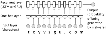
Figure 1: Simple example of recurrent neural network.

The parameters of the neural network (composed of the weights of the recurrent units and those of the final output layer) are learned from training data. To this end, the neural network is provided with a dataset of (input, output) pairs, and an optimisation algorithm (such as stochastic gradient descent) is then applied to find the parameters that minimise the empirical loss on this dataset (see Goodfellow et al. (2016) for more details). In this particular case, the network is trained using both examples of malware-generated domains (for which the output produced by the network should be as close to 1 as possible) as well as examples of benign domains (for which the output should be close to 0). Section 4 describes the datasets that have been employed in this work.

3.2 Extensions

Starting from the core architecture described above, we can then extend or modify the neural network in several ways:

Embeddings

Instead of adopting a one-hot representation, we can use a learnable embedding model to convert each character into a dense vector (Goldberg, 2016). One advantage of embedding models is their ability to express similarities between characters – for instance, the vector for the character ’0’ will be closer in vector space to the character ’3’ than to ’u’, since the distributional properties of ’0’ are more similar to ’3’ than to ’u’. These embeddings can be learned simultaneously with the other network parameters.

Bidirectionality

The network in Figure 1 operates only in a left to right fashion. However, recurrent neural networks can be easily extended to work in both directions (Schuster and Paliwal, 1997), as shown in Figure 3. This allows the network to capture underlying patterns that might appear in both directions.

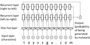
Figure 2: Bidirectional recurrent neural network.

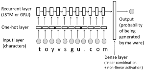
Figure 3: Recurrent neural network with an additional dense layer.

Additional dense layer

Instead of computing the final output directly from the hidden state of the last recurrent unit, one might first pass it through a dense feed-forward layer, such as depicted in Figure 3. The dense layer is a linear combination of the inputs followed by a non-linear activation function. The inclusion of this additional layer may help improve the model performance by applying a non-linear transformation to the state vector capturing the sequence of characters making up the domain name. However, this also increases the size of the parameter space: if the size of the state vector is $K$ and the size of the dense layer is $L$, an additional $(L+1)\times K$ parameters will need to be learned.

Multi-task learning

Neural models need not be restricted to the mere detection of malicious domain names, but can also be used predict the type of malware (for instance, suppobox) it belongs to. In this case, the network must output a probability distribution over malware classes (augmented with one class for the “benign” domains). This classification can be achieved in a separate neural network or be integrated in a single, unified network, as shown in Figures 5 and 5. This unified network is an instance of multi-task architectures (Ruder, 2017), since the model is optimised to perform two tasks at once, namely predicting whether the domain is malicious, and which malware it comes from.

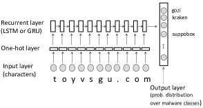
Figure 4: Recurrent neural network for predicting the malware classes.

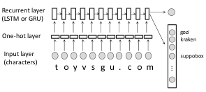
Figure 5: Recurrent neural network for simultaneous detection & classification.

The influence of these design choices is evaluated in Section 5.

4 Datasets

Training neural models requires access to large amounts of examples, both positive (domains known to have been generated by a DGA) and negative (domains known as benign). The following datasets were used for this purpose:

4.0.1 Benign domains

The benign domains were extracted from domain whitelists. We downloaded eight snapshots of the Alexa Top 1 million domains (spread from 2010 to 2017), along with similar whitelists such as the top 1 million from Statvoo and Cisco. In total, over 4 million benign domains were extracted from these domain lists. One should note that the Alexa rankings only enumerate popular domains and offers no guarantee that the domains are malware-free. However, in practice, DGA-generated domains have a very low probability of appearing on these ranked lists due to their random and transient character.

4.0.2 Malware domains

The malware-generated domains is compiled from three complementary sources. The most important source is the DGArchive, which is a web service for malware analysis. The DGAarchive contains regularly updated datasets and technical details for dozens of malware families. The administrators of DGArchive kindly provided us with a complete dump of their malware database, which amounts to an initial set of over 49 million malware domains spread over 63 distinct types of malware.

The number of examples for each family is, however, heavily skewed. For instance, the virut malware contains more than 17 million examples (although its algorithm is relatively straightforward to capture), while a difficult malware such as matsnu only contains 12.7 thousand examples. To counter this class imbalance, we divided the malware families in two groups according to their detection difficulty. The maximal number of examples was capped to 40 000 for “easy” malware families and to 400 000 for difficult ones. In addition to the DGArchive, we also extracted the DGA feeds from Bambenek Consulting, containing 39 malware families and used domain generators for 11 DGAs to produce additional examples of domains.

Due to the lack of authoritative naming conventions for malware, there is some variation in the DGA names depending on the source (for instance, the emotet malware is often referred to as geodo). We therefore created a list of equivalent names for each DGA in order to merge all malware domains into a single list. To reduce the amount of noise in the dataset, also excluded from the training examples the few domains that were simultaneously marked as benign and malware. The complete list of malware names along with their number of examples is provided in Table 1. The combination of all sources yields a total of 2.9 million malware-generated domains.

Malware	Frequency
bamital	40 240		gozi	105 631		ramdo	15 984
banjori	89 984		hesperbot	370		ramnit	90 000
bedep	15 176		locky	179 204		ranbyu	40 000
beebone	420		madmax	192		ranbyus	12 720
blackhole	732		matsnu	12 714		rovnix	40 000
bobax	19 288		modpack	52		shifu	4 662
conficker	400 000		murofet	53 260		simda	38 421
corebot	50 240		murofetw	40 000		sisron	5 936
cryptolocker	55 984		necur	40 000		suppobox	41 014
cryptowall	94		necurs	36 864		sutra	9 882
dircrypt	11 110		nymaim	186 653		symmi	40 064
dnschanger	40 000		oderoor	3 833		szribi	16 007
downloader	60		padcrypt	35 616		tempedreve	453
dyre	47 998		proslikefan	75 270		tinba	80 000
ekforward	1 460		pushdo	176 770		torpig	40 000
emotet	40 576		pushdotid	6 000		tsifiri	59
feodo	192		pykspa	424 215		urlzone	34 536
fobber	2 600		pykspa2	24 322		vawtrak	1 050
gameover	80 000		qadars	40 400		virut	400 600
gameover_p2p	41 000		qakbot	90 000		volatilecedar	1 494
						xxhex	4400
						Total	2 925 168

Table 1: Malwares in the dataset along with their number of example domains. The dataset is put together from malware feeds, the DGArchive, and generation scripts.

5 Evaluation

The models described in Section 3 were trained using the datasets from Section 4 and were then evaluated on the basis of their ability to distinguish between benign domain names and domain names generated by malware. This evaluation was performed using $10$-fold stratified cross validation on the full dataset. The neural models were trained on GPU-accelerated hardware (with a training time of about 3 hours) using a batch size of 256 and two passes on the training set. RMSProp was employed as optimisation algorithm. The source code for training and evaluating the neural models was written using Keras (Chollet et al., 2015) and can be provided upon request.

5.1 Baseline

Letter combinations are often good indicators of the “naturalness” of a given domain name. For instance, numbers are rarely followed by letters. Following Woodbridge et al. (2016), one can build a classifier using as features the occurrences of particular character bigrams (that is, pairs of consecutive characters) in the domain name. For instance, the domain toyvsgu.com has a total of 10 non-zero features (to, oy, …om).

Based on this observation, one can estimate a simple but effective baseline model that detects and classifies domain names based on the character pairs occurring in it. This baseline model can be expressed as a logistic regression classifier with a feature space corresponding to the set of possible character bigrams (1504 in our dataset).

5.2 Metrics

One straightforward indicator of the model performance is the confusion matrix, which can be structured in a simple table, as shown below:

		Classified by model as:
		Malware	Benign
Actual class:	Malware	True Positives (TP)	False Negatives (FN)
	Benign	False Positives (FP)	True Negatives (TN)

The following metrics can be defined based on this confusion matrix:

Accuracy

the accuracy is simply the fraction of domains that are correctly classified:

$$acc=\frac{TP+TN}{TP+TN+FN+FP}$$ (1)

However, the accuracy is not the most useful metric for this task due to its sensitivity to class imbalance. The number of benign domains in DNS traffic is likely to be orders of magnitude larger than the number of malware-generated domains. Achieving high accuracy in such situations is not particularly difficult, as one can simply create a dummy classifier that classifies all domains as benign.

Precision, Recall, $F_{1}$ score

The precision is the fraction of domains classified by the model as malware that are actually malware, while the recall (also called sensitivity or true positive rate) is the fraction of malware domains that are classified as malware by the model. Finally, the $F_{1}$ score is an harmonic mean of the two:

$$p=\frac{\text{TP}}{\text{TP}+\text{FP}}=\frac{\text{\# correctly classified malware domains}}{\text{\# domains classified as malware by model}}$$ (2)

$$r=\frac{\text{TP}}{\text{TP}+\text{FN}}=\frac{\text{\# correctly classified malware domains}}{\text{\# actual known malware domains}}$$ (3)

$$F_{1}=2\frac{p\times r}{p+r}$$ (4)

5.3 Model selection

Section 3 introduced a number of design choices regarding the architecture of the neural network. We performed an empirical evaluation of these choices, detailed below.

Inclusion of embedding models:

We found that the use of simple one-hot representations gave better results than learned character embeddings (about 1 % difference in micro $F_{1}$ score on average).

Type and dimension of recurrent units

: The detection and classification performance of GRU and LSTM units were roughly the same. However, LSTM units are slower due to their more complex gating mechanism. The output dimension was an important factor: we experimented with sizes 128, 256, 512 and 1024, and found that the best results were achieved with 512 dimensions (with a 1 % increase in micro $F_{1}$ score compared to the lower dimensions).

Bidirectionality

: The inclusion of a right-to-left layer did slightly improve the results, but essentially because it effectively doubles the output vector dimensions. When compared to unidirectional networks with the same total number of dimensions, bidirectional networks do not seem to perform better and are slower to run.

Use of additional hidden layer

: The inclusion of a dense layer between the last recurrent unit and the output prediction did not improve the performance.

Multi-task learning

The use of the same neural network to both detect whether a domain name is DGA-generated and which class it belong to gave approximately the same empirical results on $F_{1}$ and AUC scores as networks optimised for these two tasks separately. This is an interesting result, as it shows that the two tasks can be performed on the basis of a shared latent representation.

On the basis of this analysis, we performed the experimental evaluation with a neural network using a one-hot input representation, 512-dimensional GRU units, no additional layer and two simultaneous outputs (detection and classification). In terms of running time, the neural model is able to process tens of thousands of domains per second on a single GPU. The model can also run on commodity hardware without GPU acceleration but is then slower, typically around one thousand domains per second.

5.4 Results

The empirical results for the detection and classification tasks are respectively shown in Table 2 and Table 3.

For the detection task, we employ the accuracy, precision, recall and $F_{1}$ score as metrics, along with the “Area Under the Curve” (AUC) metric. The ROC curse illustrates the evolution of the true positive and false positive rates at various thresholds, and is shown in Figure 6. Contrary to the accuracy, the AUC score is well suited to machine learning tasks where the classes are highly imbalanced. As we can observe from Table 2, the neural model outperforms the two baseline on all metrics (all results are statistically significant using a paired $t$-test, with $p<0.0001$). Another way of interpreting the results is to look at the ROC curve and determine the detection rate that can be achieved for a given False Positive Rate (FPR). The neural model is able to detect 68 % of malwared-generated domain names for a FPR of 1:1000 (compared to only 23 % for the bigram approach), 93 % for a FRP of 1:100, and 99.9 % for a FPR of 1:10.

	Accuracy	Precision	Recall	$F_{1}$ score	ROC AUC
Bigram	0.915	0.927	0.882	0.904	0.970
Neural model	0.973	0.972	0.970	0.971	0.996

Table 2: Evaluation results (with 10-fold cross validation) on the task of detecting malware-generated domain names, using the dataset described in Section 4.

	Accuracy	Precision		Recall		$F_{1}$ score
		Micro	Macro	Micro	Macro	Micro	Macro
Bigram	0.800	0.787	0.564	0.800	0.513	0.787	0.522
Neural model	0.892	0.891	0.713	0.892	0.653	0.887	0.660

Table 3: Evaluation results (with 10-fold cross validation) on the task of classifying domain names according to the malware family that generated it (including the 63 malware types and a special “benign” family).

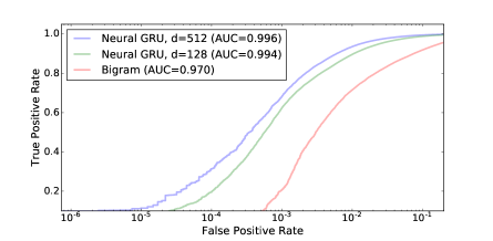
Figure 6: ROC curve for the detection task ($x$-axis is in log-scale).

	Detection		Classification
	Bigram	Neural	Bigram			Neural
Malware	Recall	Recall	Precision	Recall	$F_{1}$ score	Precision	Recall	$F_{1}$ score
bamital	0.991	1.000	0.999	0.998	0.998	0.999	0.999	0.999
banjori	0.893	1.000	0.910	0.928	0.919	0.993	0.999	0.996
bedep	0.985	0.991	0.024	0.006	0.010	0.798	0.584	0.672
beebone	0.000	0.952	0.467	0.065	0.112	0.426	0.418	0.421
benign	0.942	0.977	0.911	0.950	0.930	0.971	0.979	0.975
blackhole	0.997	0.995	0.000	0.000	0.000	0.783	0.281	0.386
bobax	0.926	0.990	0.666	0.549	0.601	0.906	0.746	0.818
conficker	0.919	0.947	0.541	0.453	0.493	0.650	0.625	0.636
corebot	0.989	1.000	0.996	0.995	0.995	0.996	0.998	0.997
cryptolocker	0.988	0.995	0.447	0.112	0.179	0.612	0.494	0.536
dircrypt	0.996	0.998	0.173	0.327	0.226	0.508	0.334	0.389
dnschanger	0.961	0.975	0.006	0.000	0.001	0.602	0.960	0.740
dyre	0.993	1.000	0.982	1.000	0.991	0.999	1.000	1.000
ekforward	0.492	0.989	0.935	0.201	0.323	0.995	0.991	0.993
emotet	0.999	0.999	0.816	0.991	0.895	0.995	0.998	0.996
feodo	1.000	1.000	0.000	0.000	0.000	0.452	0.189	0.262
fobber	0.978	0.989	0.000	0.000	0.000	0.662	0.185	0.276
gameover	0.998	1.000	0.958	0.971	0.965	0.999	0.998	0.999
gameover_p2p	1.000	1.000	0.901	0.915	0.908	0.945	0.939	0.942
gozi	0.398	0.879	0.816	0.682	0.743	0.909	0.874	0.889
hesperbot	0.932	0.949	0.000	0.000	0.000	0.000	0.000	0.000
locky	0.954	0.980	0.592	0.535	0.562	0.733	0.675	0.699
madmax	0.923	0.660	0.000	0.000	0.000	0.095	0.035	0.051
matsnu	0.046	0.158	0.036	0.003	0.005	0.683	0.103	0.172
murofet	0.998	0.998	0.552	0.528	0.539	0.737	0.838	0.784
murofetweekly	1.000	1.000	0.976	1.000	0.988	0.973	0.998	0.985
necur	0.957	0.982	0.397	0.245	0.302	0.475	0.490	0.461
necurs	0.962	0.982	0.317	0.151	0.204	0.431	0.248	0.278
nymaim	0.924	0.953	0.601	0.254	0.357	0.613	0.391	0.475
oderoor	0.926	0.977	0.000	0.000	0.000	0.196	0.034	0.055
padcrypt	0.970	0.999	0.990	0.999	0.994	0.996	0.998	0.997
proslikefan	0.913	0.960	0.501	0.272	0.353	0.829	0.385	0.526
pushdo	0.907	0.993	0.947	0.940	0.943	0.986	0.993	0.990
pushdotid	0.913	0.968	0.321	0.102	0.154	0.869	0.946	0.905
pykspa	0.945	0.983	0.507	0.671	0.578	0.683	0.862	0.761
pykspa2	0.902	0.992	0.616	0.647	0.631	0.680	0.895	0.772
qadars	0.978	0.999	0.997	0.999	0.998	0.993	0.995	0.994
qakbot	0.991	0.994	0.650	0.329	0.436	0.827	0.481	0.608
ramdo	0.986	1.000	0.828	0.878	0.852	0.995	0.918	0.955
ramnit	0.976	0.981	0.454	0.539	0.493	0.557	0.617	0.585
ranbyu	0.997	0.999	0.500	0.260	0.342	0.643	0.757	0.688
ranbyus	0.997	0.997	0.000	0.000	0.000	0.268	0.143	0.175
rovnix	0.993	0.999	0.873	0.645	0.742	0.993	0.990	0.991
shifu	0.942	0.983	0.007	0.003	0.004	0.327	0.110	0.137
simda	0.660	0.985	0.850	0.852	0.851	0.960	0.983	0.971
sisron	1.000	1.000	0.998	1.000	0.999	1.000	0.999	1.000
suppobox	0.125	0.931	0.666	0.581	0.621	0.913	0.925	0.917
sutra	0.999	0.999	0.888	0.906	0.897	0.976	0.987	0.981
symmi	0.940	0.996	0.989	1.000	0.994	0.997	0.997	0.997
szribi	0.891	0.991	0.695	0.711	0.703	0.952	0.987	0.969
tempedreve	0.881	0.937	0.000	0.000	0.000	0.241	0.010	0.019
tinba	0.990	0.996	0.599	0.606	0.602	0.816	0.926	0.866
torpig	0.916	0.997	0.775	0.832	0.802	0.982	0.993	0.988
urlzone	0.951	0.991	0.531	0.388	0.448	0.982	0.896	0.937
vawtrak	0.862	0.906	0.000	0.000	0.000	0.743	0.363	0.455
virut	0.666	0.942	0.565	0.758	0.647	0.882	0.933	0.907
volatilecedar	0.317	0.954	0.982	0.977	0.979	0.987	0.964	0.974
xxhex	0.832	0.999	0.983	0.997	0.990	0.999	0.999	0.999

Table 4: Detection and classification results for each malware family (and benign class). For the detection task, only the recall is provided, since precision is not applicable.

For the classification task, the employed metrics are the accuracy, precision, recall and $F_{1}$ scores. Since the precision, recall and $F_{1}$ scores are class-specific measures, they must be averaged to yield a global result. Micro-averages sum up the individual TP, FP and FN for all classes, while macro-averages take the mean of the individual scores for all classes. In other words, micro-averages take into account the relative weights (in terms of number of examples) of all classes, while macro-averages do not. As shown in Table 3, the neural model also outperforms the two baselines on all metrics.

We can refine the analysis of the empirical results by looking at detection and classification results for each malware family, as illustrated in Table 4. One interesting result of this evaluation is the ability of the neural model to detect dictionary-based DGAs such as suppobox (with a recall of 0.931 for the neural model compared to 0.125 for the bigram model), provided the number of training examples is sufficient. In other words, the neural model was capable of “learning” the wordlists employed by the the DGA, which is something that earlier approaches based on character statistics are unable to do. However, some domain-generation algorithms remain difficult to detect, such as matsnu (with a recall of only 0.158). matsnu is a dictionary-based DGA relying on a built-in list of more than 1 300 verbs and nouns. As the dataset used for the evaluation only contains 12 714 examples of matsnu domains, this was probably insufficient to learn the underlying regularities produced by this DGA.

6 Conclusion

This paper presented a data-driven approach to the automatic detection of malware-generated domain names using recurrent neural networks. Although the idea of using recurrent neural networks for detecting malicious domains is not entirely new (Woodbridge et al., 2016), the paper is to our knowledge the first one to evaluate it on a large dataset of several million malware-generated domains (covering a total of 61 malware families). The model does not require any handcrafted feature and can be easily retrained to respond to new malwares. Furthermore, it can be directly applied on the raw domain names, without requiring access to additional contextual information.

Future work will investigate the integration of this neural model as part of a larger machine-learning architecture for the detection of cyber-threats in traffic data.

References

- Anderson et al. (2016) H. S. Anderson, J. Woodbridge, and B. Filar. DeepDGA: Adversarially-tuned domain generation and detection. In Proceedings of the 2016 ACM Workshop on Artificial Intelligence and Security, pages 13–21. ACM, 2016.
- Antonakakis et al. (2012) M. Antonakakis, R. Perdisci, Y. Nadji, N. Vasiloglou, S. Abu-Nimeh, W. Lee, and D. Dagon. From throw-away traffic to bots: Detecting the rise of DGA-based malware. In USENIX security symposium, volume 12, 2012.
- Bahdanau et al. (2014) D. Bahdanau, K. Cho, and Y. Bengio. Neural machine translation by jointly learning to align and translate. arXiv e-prints, abs/1409.0473, September 2014.
- Barabosch et al. (2012) T. Barabosch, A. Wichmann, F. Leder, and E. Gerhards-Padilla. Automatic extraction of domain name generation algorithms from current malware. In Proc. NATO Symposium IST-111 on Information Assurance and Cyber Defense, Koblenz, Germany, 2012.
- Chollet et al. (2015) F. Chollet et al. Keras. https://github.com/fchollet/keras, 2015.
- Chung et al. (2014) J. Chung, Ç Gülçehre, K. Cho, and Y. Bengio. Empirical evaluation of gated recurrent neural networks on sequence modeling. CoRR, abs/1412.3555, 2014.
- Goldberg (2016) Y. Goldberg. A primer on neural network models for natural language processing. Journal of Artificial Intelligence Research (JAIR), 57:345–420, 2016.
- Goodfellow et al. (2016) I. Goodfellow, Y. Bengio, and A. Courville. Deep Learning. MIT Press, 2016.
- Graves et al. (2013) A. Graves, A. Mohamed, and G. E. Hinton. Speech recognition with deep recurrent neural networks. In IEEE International Conference on Acoustics, Speech and Signal Processing (ICASSP 2013), pages 6645–6649, 2013.
- Grill et al. (2015) M. Grill, I. Nikolaev, V. Valeros, and M. Rehak. Detecting DGA malware using netflow. In Integrated Network Management (IM), 2015 IFIP/IEEE International Symposium on, pages 1304–1309. IEEE, 2015.
- Hochreiter and Schmidhuber (1997) S. Hochreiter and J. Schmidhuber. Long short-term memory. Neural Computation, 9(8):1735–1780, November 1997. ISSN 0899-7667.
- Kührer et al. (2014) M. Kührer, C. Rossow, and T. Holz. Paint it black: Evaluating the effectiveness of malware blacklists. In International Workshop on Recent Advances in Intrusion Detection, pages 1–21. Springer, 2014.
- Plohmann et al. (2016) D. Plohmann, K. Yakdan, M. Klatt, J. Bader, and E. Gerhards-Padilla. A comprehensive measurement study of domain generating malware. In 25th USENIX Security Symposium (USENIX Security 16), pages 263–278, 2016.
- Ruder (2017) S. Ruder. An overview of multi-task learning in deep neural networks. CoRR, abs/1706.05098, 2017.
- Schiavoni et al. (2014) S. Schiavoni, F. Maggi, L. Cavallaro, and S. Zanero. Phoenix: DGA-based botnet tracking and intelligence. In International Conference on Detection of Intrusions and Malware, and Vulnerability Assessment, pages 192–211, 2014.
- Schuster and Paliwal (1997) M. Schuster and K.K. Paliwal. Bidirectional recurrent neural networks. IEEE Transactions on Signal Processing, 45(11):2673–2681, November 1997.
- Villamarin-Salomon and Brustoloni (2008) R. Villamarin-Salomon and J. C. Brustoloni. Identifying botnets using anomaly detection techniques applied to DNS traffic. In Consumer Communications and Networking Conference, 2008. CCNC 2008. 5th IEEE, pages 476–481. IEEE, 2008.
- Vinyals and Le (2015) O. Vinyals and Q. Le. A Neural Conversational Model. CoRR, abs/1506.05869, 2015.
- Woodbridge et al. (2016) J. Woodbridge, H. S Anderson, A. Ahuja, and D. Grant. Predicting domain generation algorithms with long short-term memory networks. arXiv preprint arXiv:1611.00791, 2016.
- Yadav and Reddy (2011) S. Yadav and AL N. Reddy. Winning with DNS failures: Strategies for faster botnet detection. In International Conference on Security and Privacy in Communication Systems, pages 446–459. Springer, 2011.
- Yadav et al. (2010) S. Yadav, A. K. K. Reddy, AL Reddy, and S. Ranjan. Detecting algorithmically generated malicious domain names. In Proceedings of the 10th ACM SIGCOMM conference on Internet measurement, pages 48–61. ACM, 2010.
- Zhou et al. (2013) Y. Zhou, Q.-S. Li, Q. Miao, and K. Yim. DGA-based botnet detection using DNS traffic. J. Internet Serv. Inf. Secur., 3(3/4):116–123, 2013.