A Flocking-based Approach for Distributed Stochastic Optimization

Abstract

In recent years, the paradigm of cloud computing has emerged as an architecture for computing that makes use of distributed (networked) computing resources. In this paper, we consider a distributed computing algorithmic scheme for stochastic optimization which relies on modest communication requirements amongst processors and most importantly, does not require synchronization. Specifically, we analyze a scheme with $N>1$ independent threads implementing each a stochastic gradient algorithm. The threads are coupled via a perturbation of the gradient (with attractive and repulsive forces) in a similar manner to mathematical models of flocking, swarming and other group formations found in nature with mild communication requirements. When the objective function is convex, we show that a flocking-like approach for distributed stochastic optimization provides a noise reduction effect similar to that of a centralized stochastic gradient algorithm based upon the average of $N$ gradient samples at each step. The distributed nature of flocking makes it an appealing computational alternative. We show that when the overhead related to the time needed to gather $N$ samples and synchronization is not negligible, the flocking implementation outperforms a centralized stochastic gradient algorithm based upon the average of $N$ gradient samples at each step. When the objective function is not convex, the flocking-based approach seems better suited to escape locally optimal solutions due to the repulsive force which enforces a certain level of diversity in the set of candidate solutions. Here again, we show that the noise reduction effect is similar to that associated to the centralized stochastic gradient algorithm based upon the average of $N$ gradient samples at each step.

1 Introduction

Swarms, flocks and other group formations can be found in nature in many organisms ranging from simple bacteria to mammals (see [20, 19, 22] for references). Such collective and coordinated behavior is believed to be effective for avoiding predators and/or for increasing the chances of finding food (foraging) (see [9, 21]). In this paper we introduce a novel distributed scheme for stochastic optimization wherein multiple independent computing threads implement each a stochastic gradient algorithm which is further perturbed by repulsive and attractive terms (a function of the relative distance between solutions). Thus, the updating of individual solutions is coupled in a similar manner to mathematical models of swarming, flocking and other group formations found in nature (see [6]). We show that this coupling endows the flocking scheme with an important robustness property as noise realizations that induce trajectories differing too much from the group average are likely to be discarded.

The performance of the single-thread stochastic gradient algorithm is highly sensitive to noise. Thus, there is a literature on estimation techniques leading to better gradient estimation often involving increasing sample size (see [2, 24] for a survey of gradient estimation techniques). When sampling is undertaken in parallel, synchronization is needed to execute the tasks that can not be executed in parallel. The speed-up obtained by parallel sampling and centralized gradient estimation is limited by overhead related to (i) time spent gathering samples (which could be significant for example in the simulation of complex systems) and (ii) synchronization. In contrast, the noise reduction obtained in a flocking-based approach with $N>1$ threads does not require synchronization since each thread only needs the information on the current solution identified by neighboring threads (where the notion of neighborhood is related to a given network topology). When sampling times are not negligible and exhibit large variation, synchronization may cause significant overhead so that real-time performance of stochastic gradient algorithm based upon the average of $N$ samples obtained in parallel is highly affected by large sampling time variability. In contrast, the real-time performance of a flocking-based implementation with $N>1$ threads may be superior as each thread can asynchronously update its solution based upon a small sample size and still reap the benefits of noise reduction stemming from the flocking discipline.

To illustrate the noise reduction property, consider the minimization of the function $f(x)=\ln(\|x\|^{2}+1)$ where $x\in\mathbb{R}^{2}$. The unique optimal solution is $x^{*}=(0,0)$. Suppose that the gradient $\nabla f(x)$ is observed with noise so that the basic iteration in a stochastic gradient descent algorithm can be written as:

$$x({k+1})=x({k})+\Gamma(k)(-\nabla f(x({k}))+\varepsilon({k})),$$

where $\Gamma({k})>0$ is the step size, and the collection $\{\varepsilon({k}):k>0\}$ is i.i.d. (independent and identically distributed) with mean zero and variance $\sigma^{2}$. The stochastic gradient method with constant step size $\Gamma(k)=0.02$ and normally distributed noise with $\sigma^{2}=450$ is unable to approximate the optimal solution given the large magnitude of noise (relative to the gradient). One solution to this conundrum is to implement an improved version based upon the average of $N=10$ samples of the gradient at each step. Then the variance of noise is reduced to ${\sigma}^{2}/N=45$. Supposing that each step takes $0.02s$, the performance of this approach is shown in Figure 1(a).

In this paper we advocate a different tack. We introduce an additional perturbation to the gradient so that the basic iteration for thread $i$ is:

$$x({i,k+1})=x({i,k})+\tilde{\Gamma}({i,k})\left[-\nabla f(x({i,k}))+\varepsilon({i,k})-\sum_{j=1,j\neq i}^{N}\alpha_{ij}\nabla_{x(i,k)}J(\|x({i,k})-x({j_{i},k})\|)\right],$$

where $J(\|x({i,k})-x(j_{i},k)\|)$ represents the flocking potential between threads $i$ and $j$. $\alpha_{ij}=1$ if thread $i$ has access to the current solution $x({j_{i},k})$ identified by thread $j$ and $\alpha_{ij}=0$ otherwise. The term $\nabla_{x(i,k)}J(\|x({i,k})-x({j_{i},k})\|)$ is a combination of repulsive and attractive “forces” depending upon the relative distance $\|x({i,k})-x({j_{i},k})\|$ (see [4] for reference). The performance of the flocking-based scheme is measured by the average solution of all threads.

Figure 1(b) depicts the performance of the flocking-discipline of $N=10$ fully connected threads (again with constant step size $\tilde{\Gamma}({i,k})=0.02$ and noise variance $\sigma^{2}=450$). It can be seen to be comparable with the scheme based upon the average of $N=10$ samples at each step. The times needed for the solutions identified by each scheme to reach the ball $B_{0.1}(x^{*})=\{x\in\mathbb{R}^{2}~{}|~{}\|x-x^{*}\|\ <0.1\}$ are fairly similar .

This noise reduction effect can be succinctly explained as follows. Under a flocking discipline, noise realizations that induce trajectories differing too much from the group average are likely to be discarded because of the attractive potential effect on each individual thread which leads to cohesion. The noise reduction enabled by a flocking-discipline is fundamentally different from that associated with the averaging of independent gradient samples.

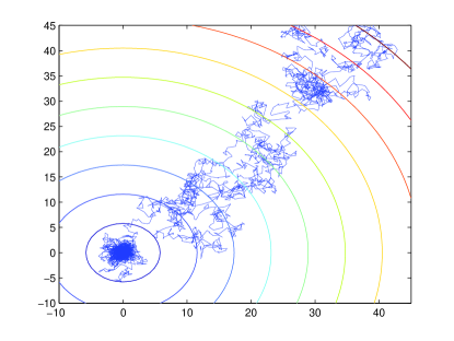
(a) Sample paths for sample average scheme with $N$ samples.

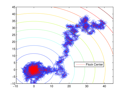
(b) Sample paths with flocking discipline ($N$ threads).

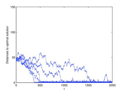
(c) Distance to optimum for sample average scheme with $N$ samples.

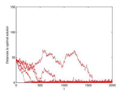
(d) Distance between the average flocking solution and the optimum.

Figure 1: Performance comparison between the scheme based upon the average of $N=10$ gradient samples per step and the flocking-based approach with $10$ fully connected threads.

Our work is related to the extensive literature in stochastic approximation method dating to [23] and [14]. These work includes the analysis of convergence (conditions for convergence, rates of convergence, proper choice of step size) in the context of diverse noise models (see [16]). Recently there has been considerable interest in parallel or distributed implementation of stochastic gradient algorithms (see [1, 26, 17, 25, 27] for examples). However, they mainly aim at minimizing a sum of convex functions which is different from our objective.

Our work is also linked with population-based algorithms for simulation-based optimization. In these approaches, at every iteration, the quality of each solution in the population is evaluated and a new population of solutions is randomly generated according to a given rule designed to achieve an acceptable trade-off between “exploration” and “exploitation” effort. Recent efforts have focused on model-based algorithms (see [12]) which differ from population-based approaches in that candidate solutions are generated at each iteration by sampling from a “model” which is a probability distribution over the solution space. The basic idea is to modify the model based on the sampled solutions in order to bias the future search towards regions containing high quality solutions (see [11] for a recent survey). These approaches are inherently centralized in that the updating of populations (or models) is undertaken after the quality of all candidate solutions is evaluated.

The structure of this paper is as follows. Section 2 introduces the optimization problem of interest. In Section 3, we perform cohesion analysis of the flocking-based approach with respect to the solutions identified by different threads. Section 4 formalizes the noise reduction properties of the flocking-based algorithmic scheme for convex optimization. In Section 5, we apply the flocking-based algorithm to the optimization of general non-convex functions. Section 6 concludes the paper.

2 Setup

2.1 Preliminaries

In the analysis of this paper we shall make use of certain graph theoretic concepts which we briefly review below. A graph $\mathcal{G}$ is a pair $(\mathcal{V},\mathcal{E})$, where $\mathcal{V}$ is a set of vertices and $\mathcal{E}$ is a subset of $\mathcal{V}\times\mathcal{V}$ called edges. A graph $(\mathcal{V},\mathcal{E})$ is called undirected if $(i,j)\in\mathcal{E}\Leftrightarrow(i,j)\in\mathcal{E}$. The adjacency matrix $A=[\alpha_{ij}]\in\mathbb{R}$ of a graph is a matrix with nonzero elements satisfying the property $\alpha_{ij}>0\Leftrightarrow(i,j)\in\mathcal{E}$. Self-joining edges are excluded, i.e., $\alpha_{ii}=0,\forall i$. The Laplacian matrix $L$ associated with a graph $(\mathcal{V},\mathcal{E})$ is defined as $L=[l_{ij}]$, where $l_{ii}=\sum_{j}\alpha_{ij}$ and $l_{ij}=-\alpha_{ij}$ where $i\neq j$. For an undirected graph, the Laplacian matrix is symmetric positive semi-definite (see [8]).

2.2 Problem Statement

We consider the problem

$$\min_{x\in\mathbb{R}^{m}}f(x)$$ (1)

where $f:\mathbb{R}^{m}\rightarrow\mathbb{R}$ is a differentiable function that is not available in closed form. To solve this problem, a black-box noisy simulation model is used. In this context, noise can have many sources such as modeling and discretization error, incomplete convergence, and finite sample size for Monte-Carlo methods (see for instance [15]). Assume that we have $N$ computing threads that can generate gradient samples in parallel. Every gradient sample is subject to i.i.d. noise $\varepsilon\in\mathbb{R}^{m}$ of mean zero and variance $\sigma^{2}$ in each dimension.

In the rest of this section, we present two algorithms for solving the problem. First, we introduce a centralized stochastic gradient-descent algorithm. Then we propose the flocking-based approach. In both cases, we assume the step size is a constant value ($\Gamma$ and $\tilde{\Gamma}$, respectively).

2.2.1 A Centralized Algorithm

A centralized stochastic gradient-descent algorithm is of the form:

$$x(k+1)=x(k)+\Gamma u(k),\ \ k\in\mathbb{N}$$ (2)

where $u(k)=-\nabla f(x(k))+\epsilon(k)$, with $\epsilon(k)$ being the random simulation noise. Assume that sampling takes place through $N$ parallel computing threads, where each thread contributes one sample in a single step. Then, $\epsilon(k)$ is given by an average of $N$ i.i.d. random vectors: $\epsilon(k)=(1/N)\sum_{i=1}^{N}\varepsilon(i)$. Each $\varepsilon(i)$ has $m$ i.i.d. components of mean zero and variance $\sigma^{2}$.

In what follows, we approximate the discrete-time process (2) by a continuous-time system for ease of analysis. Let $\Delta t(k)$ be the time needed to gather $N$ samples for calculating $u(k)$. Then solution $x(k)$ is obtained at $t(k)=\sum_{l<k}\Delta t(l)$ in continuous-time. Denoting by $x_{t}$ the identified solution at time $t$, we have $x_{t(k)}=x(k)$ and $x_{t}=x(k-1)$ for all $t\in(t(k-1),t(k))$, i.e., the continuous-time solution changes discretely. By scheme (2),

$$x_{t}=x_{0}-\sum_{t(l)<t}\nabla f(x_{t(l)})\Gamma+\sum_{t(l)<t}\epsilon(l)\Gamma.$$

Define a new variable $y_{t}:=x_{t/\Gamma}$. It follows that

$$y_{t}=x_{0}-\sum_{t(l)<t/\Gamma}\nabla f(x_{t(l)})\Gamma+\sum_{t(l)<t/\Gamma}\epsilon(l)\Gamma=y_{0}-\sum_{\Gamma t(l)<t}\nabla f(y_{\Gamma t(l)})\Gamma+\sum_{t(l)<t/\Gamma}\epsilon(l)\Gamma.$$

Assume that all $\Delta t(k)$’s are i.i.d. with mean $\mathbb{E}[\Delta t(k)]=\Delta t$, and let $n_{t}$ be the cardinality of $\{l:\Gamma t(l)<t\}$. By the (strong) law of large numbers, for small $\Gamma>0$,

$$\frac{\Gamma n_{t}}{t}=\frac{n_{t}}{t/\Gamma}\simeq\frac{1}{\Delta t},\;\text{and}\;\frac{n_{t}}{t}\gg 0.$$ (3)

Hence,

$$\sum_{\Gamma t(l)<t}\nabla f(y_{\Gamma t(l)})\Gamma=\frac{\Gamma n_{t}}{t}\left[\sum_{\Gamma t(l)<t}\nabla f(y_{\Gamma t(l)})\frac{t}{n_{t}}\right]\simeq\frac{\Gamma n_{t}}{t}\int_{0}^{t}\nabla f(y_{t})dt\simeq\frac{1}{\Delta t}\int_{0}^{t}\nabla f(y_{t})dt.$$

Note that $\sum_{t(l)<t/\Gamma}\epsilon(l)\Gamma$ has mean zero and variance $\Gamma^{2}n_{t}\sigma^{2}/N$ in each dimension. In light of (3),

$$\frac{\Gamma^{2}n_{t}\sigma^{2}}{N}=\frac{\Gamma n_{t}}{t}\Delta t\frac{\Gamma\sigma^{2}t}{N\Delta t}\simeq\frac{\Gamma\sigma^{2}}{N\Delta t}t.$$

We have

$$\sum_{t(l)<t/\Gamma}\epsilon(l)\Gamma\simeq\sigma\sqrt{\frac{\Gamma}{N\Delta t}}B_{t},$$

where $B_{t}$ is the standard $m$-dimensional Brownian motion.

Define $\gamma=1/\Delta t$ and $\tau_{N}=\sigma\sqrt{{\Gamma\Delta t}/{N}}$. Then $y_{t}$ approximately satisfies the following stochastic Ito integral:

$$y_{t}=y_{0}-\gamma\int_{0}^{t}\nabla f(y_{t})dt+\int_{0}^{t}\tau_{N}\gamma dB_{t}.$$

which is usually written in its differential form:

$$dy_{t}=-\nabla f(y_{t})\gamma dt+\tau_{N}\gamma dB_{t}.$$ (4)

2.2.2 A Flocking-based Algorithm

A flocking-based implementation also has $N$ computing threads. In contrast to the centralized approach, each thread $i$ independently implement a stochastic gradient algorithm based on only one sample at each step:

$$x(i,k+1)=x(i,k)+\tilde{\Gamma}u(i,k),\ \ k\in\mathbb{N}$$ (5)

where

$$u(i,k)=-\nabla f(x(i,k))+\varepsilon({i,k})-\sum_{j=1,j\neq i}^{N}\alpha_{ij}\nabla_{x(i,k)}J(\|x(i,k)-x(j_{i},k)\|).$$

Here $x(j_{i},k)$ denotes the current solution of thread $j\neq i$ at the time of thread $i$’s update, and noise term $\varepsilon({i,k})$ comes from one sampling. Thus each $\varepsilon({i,k})$ is i.i.d. with $m$ i.i.d. components of mean zero and variance $\sigma^{2}$.

The additional term $-\sum_{j=1,j\neq i}^{N}\alpha_{ij}\nabla_{x_{i}}J(\|x(i,k)-x(j_{i},k)\|)$ represents the function of mutual attraction and repulsion between individual threads (see [5] for reference). $A=[\alpha_{ij}]\in\mathbb{R}^{N\times N}$ is the coupling matrix with $\alpha_{ij}\in\{0,1\}$. $\alpha_{ij}=1$ indicates that thread $i$ is informed of the solution identified by threads $j$. We assume that the corresponding graph $\mathcal{G}$ is undirected ($A=A^{T}$) and connected.

Denote with $\Delta t({i,k})$ the time needed by thread $i$ to gather one sample for $u(i,k)$, then $x({i,k})$ is obtained at time $t(i,k)=\sum_{l<k}\Delta t({i,l})$. Let $x_{i,t}$ be the solution of thread $i$ at time $t$. It satisfies $x_{t(i,k)}=x(i,k)$ and $x_{i,t}=x(i,k-1)$ for all $t\in(t(i,k-1),t(i,k))$. The scheme can be written as follows: for each thread $i\in\{1,\ldots,N\}$,

$$x_{i,t(i,k+1)}=x_{i,t(i,k)}+\tilde{\Gamma}\left[-\nabla f(x_{i,t(i,k)})+\varepsilon({i,k})-\sum_{j=1,j\neq i}^{N}\alpha_{ij}\nabla_{x_{i,t(i,k)}}J(\|x_{i,t(i,k)}-x_{j,t(i,k)}\|)\right].$$

Define function $g(\cdot)$ as $g(x)=-\nabla_{x}J(\|x\|)$. Let $y_{i,t}=x_{i,t/\tilde{\Gamma}}$ and assume all $\Delta t({i,k})$’s are i.i.d. with $\mathbb{E}[\Delta t({i,k})]=\tilde{\Delta}t$. Similar to (4), for small $\tilde{\Gamma}>0$ the dynamics of $y_{i,t}$ can be approximated by

$$dy_{i,t}=\left[-\nabla f(y_{i,t})+\sum_{j=1,j\neq i}^{N}\alpha_{ij}g(y_{i,t}-y_{j,t})\right]\tilde{\gamma}dt+\tau\tilde{\gamma}dB_{i,t},$$ (6)

where $\tilde{\gamma}=1/\tilde{\Delta}t$ and $\tau=\sigma\sqrt{{\tilde{\Gamma}\tilde{\Delta}t}}$.

In this paper, we characterize the performance of the flocking-based approach using the average solution $\bar{x}_{t}=({1}/{N})\sum\nolimits_{i=1}^{N}x_{i,t}$.

Remark 1.

In what follows, we shall use the same specification for $g(\cdot)$ as in [5], i.e., $g(\cdot)$ is an odd function of the form:

$$g(x)=-x[g_{a}(\|x\|)-g_{r}(\|x\|)],$$ (7)

where $g_{a}:\mathbb{R}^{+}\rightarrow\mathbb{R}^{+}$ represents (the magnitude of) the attraction term and it has long range, whereas $g_{r}:\mathbb{R}^{+}\rightarrow\mathbb{R}^{+}$ represents (the magnitude of) the repulsion term and it has short range, and $\|\cdot\|$ is the Euclidean norm. We assume that $J(\cdot)$ has a unique minimizer, and there is an equilibrium distance $\rho>0$ such that $g_{a}(\rho)=g_{r}(\rho)$, and for $\|x\|>\rho$ we have $g_{a}(\|x\|)>g_{r}(\|x\|)$, and for $\|x\|<\rho$ we have $g_{a}(\|x\|)<g_{r}(\|x\|)$. In this work we consider linear attraction functions, i.e., $g_{a}(\|x\|)=a$ for some $a>0$ and all $\|x\|$, and repulsion functions satisfying $g_{r}(\|x\|)\|x\|^{2}\leq b$ uniformly for some $b>0$.

The choice of parameters $a$ (i.e. attraction) and $b$ (i.e. repulsion) reflects the emphasis on exploration (higher values of $b$) versus exploitation (higher values of $a$). The potential function is reminiscent of penalty function methods for constrained optimization in which the gradient of the objective function is perturbed so as to ensure updated solutions remain within the feasible region. The difference is that in the flocking approach, potential-induced attraction/repulsion forces keep the updated solutions in a moving ball with fixed size rather than a rigid region. In light of its functionality, the analysis would not change much if we had adopted a different potential function.

3 Analysis

In this section we study the stochastic processes $\{y_{i,t}:t\geq 0\}$ associated with each one of the $N>1$ threads in the flocking-based approach. The average solution $\bar{y}_{t}=({1}/{N})\sum\nolimits_{i=1}^{N}y_{i,t}$ will be of particular importance in characterizing the performance of the flocking-based approach. This part of the analysis pertains to a characterization of cohesiveness of the solutions identified by the different threads. To this end, we will analyze the process $\{\overline{V}_{t}:t>0\}$ defined as

$$\overline{V}_{t}=\frac{1}{N}\sum_{i=1}^{N}\frac{1}{2}\|y_{i,t}-\bar{y}_{t}\|^{2}.$$

In the analysis, we will frequently make use of Ito’s Lemma as stated below (see [18]).

Lemma 1.

(Ito’s lemma) Let

$$dX_{t}=udt+vdB_{t}$$

be an $n$-dimensional Ito process . Let $g_{t,x}$ be a twice differentiable map from $[0,\infty)\times\mathbb{R}^{n}$ into $\mathbb{R}$. Then the process

$$Y_{t}=g_{t,X_{t}}$$

is again an Ito process with

$$dY_{t}=\frac{\partial g}{\partial t}dt+\sum_{i}\frac{\partial g}{\partial x_{i}}dX_{i}+\frac{1}{2}\sum_{i,j}\frac{\partial^{2}g}{\partial x_{i}\partial x_{j}}dX_{i}dX_{j}$$

where $dB_{i}dB_{j}=\delta_{ij}dt$ ($\delta_{ij}=1$ if $i=j$ and $\delta_{ij}=0$ otherwise), $dB_{i}dt=dtdB_{i}=0$.

3.1 Preliminaries

We consider the stochastic differential equation governing $\overline{V}_{t}$. Let $V_{i,t}=({1}/{2})\|e_{i,t}\|^{2}$ with $e_{i,t}=y_{i,t}-\bar{y}_{t}$. We have $\overline{V}_{t}=({1}/{N})\sum_{i=1}^{N}V_{i,t}$. Applying Ito’s lemma,

$$d{V_{i,t}}=d{e_{i,t}}\cdot e_{i,t}+\frac{1}{2}de_{i,t}\cdot de_{i,t},$$

where $d{e_{i,t}}=d{y}_{i,t}-d{\overline{y}_{t}}$.

Lemma 2.

Suppose relation (6) holds, and assume a linear attraction function $g_{a}(\|x\|)=a$. Then $\overline{V}_{t}$ satisfies

$$d\overline{V}_{t}= -\frac{a}{N}\sum_{i=1}^{N}\sum_{j=1,j\neq i}^{N}\alpha_{ij}(e_{i,t}-e_{j,t})^{T}e_{i,t}\tilde{\gamma}dt+\frac{1}{2N}\sum_{i=1}^{N}\sum_{j=1,j\neq i}^{N}\alpha_{ij}g_{r}(\|y_{i,t}-y_{j,t}\|)\|y_{i,t}-y_{j,t}\|^{2}\tilde{\gamma}dt$$

$$-\frac{1}{N}\sum_{i=1}^{N}\nabla^{T}f(y_{i,t})e_{i,t}\tilde{\gamma}dt+\frac{\tau}{N}\tilde{\gamma}\sum_{i=1}^{N}{dB_{i,t}}^{T}e_{i,t}+\frac{m\tau^{2}\tilde{\gamma}^{2}(N-1)}{2N}dt.$$ (8)

Proof.

See Appendix 7.2. ∎

3.2 Cohesiveness

Let $L=[l_{ij}]$ be the Laplacian matrix associated with the adjacency matrix $A$. Notice that

$$-\sum_{i=1}^{N}\sum_{j=1,j\neq i}^{N}\alpha_{ij}(e_{i,t}-e_{j,t})^{T}e_{i,t}=\sum_{i=1}^{N}\sum_{j=1}^{N}l_{ij}(e_{i,t}-e_{j,t})^{T}e_{i,t}=-\sum_{i=1}^{N}\sum_{j=1}^{N}l_{ij}e_{j,t}^{T}e_{i,t}.$$ (9)

Let $\mathbf{e}_{t}=[e_{1,t}^{T},\ldots,e_{N,t}^{T}]^{T}$. Since graph $\mathcal{G}$ is connected, $\lambda_{2}(L)>0$ (see [8]) and

$$\sum_{i=1}^{N}\sum_{j=1}^{N}l_{ij}e_{j,t}^{T}e_{i,t}=\mathbf{e}_{t}^{T}(L\otimes I_{m})\mathbf{e}_{t}\geq\lambda_{2}\mathbf{e}_{t}^{T}\mathbf{e}_{t}=\lambda_{2}\sum_{i=1}^{N}\|e_{i,t}\|^{2}.$$ (10)

Here $\lambda_{2}:=\lambda_{2}(L)$ is the second-smallest eigenvalue of $L$, also called the algebraic connectivity of $\mathcal{G}$.

We make the following standing assumptions.

Assumption 1.

(Bounded gradient) There exists $\eta>0$ such that $\|\nabla f(x)\|\leq\eta$ for all $x$.

Assumption 2.

(Strong convexity) $(\nabla f(x)-\nabla f(x^{\prime}))^{T}(x-x^{\prime})\geq\kappa\|x-x^{\prime}\|^{2}$ for some $\kappa>0$ and for all $x,x^{\prime}$.

The following result provides a characterization of degree of cohesiveness of sample paths associated with different individual threads.

Theorem 1.

Suppose relation (6) holds, and assume a linear attraction function $g_{a}(\|x\|)=a$ and a repulsion function satisfying $g_{r}(\|x\|)\|x\|^{2}\leq b$. Then the ensemble average of $\overline{V}_{t}$ is uniformly bounded in $t$ under either Assumption 1 or Assumption 2. In particular,

1. If Assumption 1 is satisfied, then

   $$\mathbb{E}[\overline{V}_{t}]\leq e^{-c_{1}\tilde{\gamma}t}\overline{V}_{0}+\frac{c_{2}}{c_{1}}(1-e^{-c_{1}\tilde{\gamma}t}).$$ (11)

   where $c_{1}\in\left(0,2a\lambda_{2}\right)$ is arbitrary, and

   $$c_{2}=\frac{\eta^{2}}{2(2a\lambda_{2}-c_{1})}+\frac{b|Tr(L)|}{2N}+\frac{m\tau^{2}\tilde{\gamma}(N-1)}{2N}.$$

   In particular,

   $$\mathbb{E}[\overline{V}_{t}]\leq\max\{\overline{V}_{0},\psi_{1}^{\ast}(N)\},$$

   and in the long run, $\mathbb{E}[\overline{V}_{t}]\leq\psi_{1}^{\ast}(N)$ where

   $$\psi_{1}^{\ast}(N)=\frac{1}{2a\lambda_{2}}{\left[\sqrt{\frac{\eta^{2}}{4a\lambda_{2}}+\frac{b|Tr(L)|}{2N}+\frac{m\tau^{2}\tilde{\gamma}(N-1)}{2N}}+\sqrt{\frac{\eta^{2}}{4a\lambda_{2}}}\right]^{2}}.$$

2. If Assumption 2 is satisfied, then

   $$\mathbb{E}[\overline{V}_{t}]\leq e^{-2(\kappa+a\lambda_{2})\tilde{\gamma}t}\overline{V}_{0}+\left[\frac{b|Tr(L)|}{4N(\kappa+a\lambda_{2})}+\frac{m\tau^{2}\tilde{\gamma}(N-1)}{4N(\kappa+a\lambda_{2})}\right]\left[1-e^{-2(\kappa+a\lambda_{2})\tilde{\gamma}t}\right].$$

   In the long run,

   $$\mathbb{E}[\overline{V}_{t}]\leq\psi_{2}^{*}(N)=\frac{b|Tr(L)|}{4N(\kappa+a\lambda_{2})}+\frac{m\tau^{2}\tilde{\gamma}(N-1)}{4N(\kappa+a\lambda_{2})}.$$

Proof.

See Appendix 7.3. ∎

Remark 2.

Note that the upper bound on the ensemble average of $\overline{V}_{t}$ is decreasing in $a$ (attraction potential) and increasing in $b$ (repulsive potential). Hence, the relative strength of these parameters implies a trade-off between exploration (less cohesive solutions) and exploitation (more cohesive solutions).

Remark 3.

Note further that the algebraic connectivity $\lambda_{2}$ is critical in determining the upper bound of $\mathbb{E}[\overline{V}_{t}]$. When $N$ is fixed, a larger $\lambda_{2}$ leads to a smaller upper bound. In a complete graph, $\lambda_{2}$ achieves its maximum value $N$, and $Tr(L)=N(N-1)$. In this situation,

$$\lim_{N\rightarrow\infty}\psi_{1}^{\ast}(N) =\lim_{N\rightarrow\infty}\frac{1}{2aN}{\left[\sqrt{\frac{\eta^{2}}{4aN}+\frac{b(N-1)}{2}+\frac{m\tau^{2}(N-1)}{2N}\tilde{\gamma}}+\sqrt{\frac{\eta^{2}}{4aN}}\right]^{2}}=\frac{b}{4a}.$$

$$\lim_{N\rightarrow\infty}\psi_{2}^{\ast}(N) =\lim_{N\rightarrow\infty}\left[\frac{b(N-1)}{4(\kappa+aN)}+\frac{m\tau^{2}\tilde{\gamma}(N-1)}{4N(\kappa+aN)}\right]=\frac{b}{4a}.$$

With a large number of threads, cohesiveness is ensured by the choice of ${b}/{a}$ governing the interplay between inter-individual attraction and repulsion.

4 Noise Reduction in Convex Optimization

In this section we formalize the noise reduction properties of the flocking-based algorithmic scheme for convex optimization. Repulsion amongst threads prevents duplication of search effort which may arise for instance, when there are multiple locally optimal solutions. Thus, for convex optimization problems, there is no need for a “repulsion” amongst individual threads and in this section we set $g_{r}(\|x\|)=0$. As we shall see below, when the underlying problem is not convex, repulsion amongst threads does facilitate the identification of a globally optimal solution.

We introduce an additional regularity assumption as follows.

Assumption 3.

(Lipschitz) $\|\nabla f(x)-\nabla f(x^{\prime})\|\leq\mu\|x-x^{\prime}\|$ for some $\mu>0$ and for all $x,x^{\prime}$.

Since $g_{r}(\|x\|)=0$, equation (2) can be simplified to

$$d\overline{V}_{t}=-\frac{a}{N}\sum_{i=1}^{N}\sum_{j=1,j\neq i}^{N}\alpha_{ij}(e_{i,t}-e_{j,t})^{T}e_{i,t}\tilde{\gamma}dt-\frac{1}{N}\sum_{i=1}^{N}\nabla^{T}f(y_{i,t})e_{i,t}\tilde{\gamma}dt+\frac{\tau}{N}\tilde{\gamma}\sum_{i=1}^{N}{dB_{i,t}}^{T}e_{i,t}\\ +\frac{m\tau^{2}\tilde{\gamma}^{2}(N-1)}{2N}dt.$$ (12)

Let us introduce a measure $U_{t}={(1/2)}\|\bar{y}_{t}-x^{\ast}\|^{2}={(1/2)}\|\bar{x}_{t/\tilde{\Gamma}}-x^{\ast}\|^{2}$, of the distance between the average solution identified by all threads at time $t/\tilde{\Gamma}$ and the unique optimal solution $x^{\ast}$. Let $F_{i,t}=({1}/{2})\|y_{i,t}-x^{\ast}\|^{2}$ and $\overline{F}_{t}=({1}/{N})\sum_{i=1}^{N}F_{i,t}$. Notice that

$$\overline{F}_{t} =\frac{1}{N}\sum_{i=1}^{N}\frac{1}{2}(y_{i,t}-\bar{y}_{t}+\bar{y}_{t}-x^{\ast})\cdot(y_{i,t}-\bar{y}_{t}+\bar{y}_{t}-x^{\ast})$$

$$=\frac{1}{N}\sum_{i=1}^{N}\frac{1}{2}\|y_{i,t}-\bar{y}_{t}\|^{2}+\frac{1}{N}\sum_{i=1}^{N}\frac{1}{2}\|\bar{y}_{t}-x^{\ast}\|^{2}+\frac{1}{N}\sum_{i=1}^{N}(y_{i,t}-\bar{y}_{t})\cdot(\bar{y}_{t}-x^{\ast})$$

$$=\overline{V}_{t}+U_{t}.$$ (13)

The following results provide a characterization of the performance of the flocking-based approach to stochastic optimization under Assumptions 2 and 3.

Lemma 3.

Suppose relation (6) and Assumptions 2 and 3 hold. Assume a linear attraction function $g_{a}(\|x\|)=a$ and a repulsion function $g_{r}(\|x\|)=0$. Then the ensemble average of $U_{t}$ is uniformly bounded:

$$\mathbb{E}[U_{t}]\leq e^{-2\kappa\tilde{\gamma}t}\left[U_{0}+\frac{(\mu-\kappa)}{a\lambda_{2}}\overline{V}_{0}\right]+\frac{m\tau^{2}\tilde{\gamma}}{4\kappa N}\left[1+\frac{(\mu-\kappa)(N-1)}{a\lambda_{2}}\right](1-e^{-2\kappa\tilde{\gamma}t}).$$

In the long-run the upper bound is:

$$\lim\sup_{t\rightarrow\infty}\mathbb{E}[U_{t}]\leq\phi^{\ast}(N)=\frac{m\tau^{2}\tilde{\gamma}}{4\kappa N}\left[1+\frac{(\mu-\kappa)(N-1)}{a\lambda_{2}}\right].$$

Proof.

See Appendix 7.4. ∎

Theorem 2.

Suppose relation (6) and Assumptions 2 and 3 hold. Assume a linear attraction function $g_{a}(\|x\|)=a$ and a repulsion function $g_{r}(\|x\|)=0$. We have

$$\frac{1}{2}\mathbb{E}[\|\overline{x}_{t}-x^{*}\|^{2}]\leq e^{-2\kappa\tilde{\gamma}\tilde{\Gamma}t}\left[U_{0}+\frac{(\mu-\kappa)}{a\lambda_{2}}\overline{V}_{0}\right]+\frac{m\tau^{2}\tilde{\gamma}}{4\kappa N}\left[1+\frac{(\mu-\kappa)(N-1)}{a\lambda_{2}}\right](1-e^{-2\kappa\tilde{\gamma}\tilde{\Gamma}t}).$$ (14)

In the long-run the upper bound is:

$$\lim\sup_{t\rightarrow\infty}\frac{1}{2}\mathbb{E}[\|\overline{x}_{t}-x^{*}\|^{2}]\leq\phi^{\ast}(N)=\frac{m\tau^{2}\tilde{\gamma}}{4\kappa N}\left[1+\frac{(\mu-\kappa)(N-1)}{a\lambda_{2}}\right].$$ (15)

Proof.

Given that $(1/2)\mathbb{E}[\|\overline{x}_{t}-x^{*}\|^{2}]=(1/2)\mathbb{E}[\|\overline{y}_{\tilde{\Gamma}t}-x^{*}\|^{2}]=\mathbb{E}[U_{\tilde{\Gamma}t}]$, the above results follow immediately from Lemma 3. ∎

Remark 4.

The convergence rate of $(1/2)\mathbb{E}[\|\overline{x}_{t}-x^{*}\|^{2}]$ is characterized by factor $2\kappa\tilde{\gamma}\tilde{\Gamma}=2\kappa\tilde{\Gamma}/\tilde{\Delta}t$, i.e., stronger convexity of $f(\cdot)$, larger step sizes, and shorter sampling times accelerate convergence.

Note that if we choose $a$ such that $a\lambda_{2}\sim N$, $\phi^{\ast}(N)\sim{1}/{N}$, then the long-run upper bound of $\mathbb{E}[\|\overline{x}_{t}-x^{*}\|^{2}]$ is monotonically decreasing in $N$. In what follows, we will show that the flocking-based approach exhibits a noise reduction property that is similar to that of a stochastic gradient algorithm based upon the average of $N$ gradient samples.

Let us assume there is no time overhead in the centralized algorithm so that $\Delta t=\tilde{\Delta}t$. Also assume $\Gamma=\tilde{\Gamma}$. It follows that $\tilde{\gamma}=\gamma$ and $\tau=\sigma\sqrt{\Gamma/\gamma}$.

The stochastic differential equation for the algorithm based upon the average of $N$ gradient samples is:

$$dy_{t}=-\nabla f(y_{t})\gamma dt+\tau_{N}\gamma dB_{t}.$$

Let $G_{t}=({1}/{2})\|y_{t}-x^{\ast}\|^{2}$. It follows that

$$dG_{t}=dy_{t}\cdot y_{t}+\frac{1}{2}dy_{t}\cdot dy_{t}=-\nabla^{T}f(y_{t})y_{t}\gamma dt+\tau_{N}\gamma{dB_{t}}^{T}y_{t}+\frac{1}{2}m\tau_{N}^{2}\gamma^{2}dt.$$ (16)

Then,

$$dG_{t}\leq-2\kappa\gamma G_{t}dt+\frac{1}{2}m\tau_{N}^{2}\gamma^{2}dt+\tau_{N}\gamma{dB_{t}}^{T}y_{t}.$$

As in the proof of Lemma 3, it can be shown that

$$\mathbb{E}[G_{t}]\leq e^{-2\kappa\gamma t}G_{0}+\frac{m\tau_{N}^{2}\gamma}{4\kappa}(1-e^{-2\kappa\gamma t})=e^{-2\kappa\gamma t}G_{0}+\frac{m\sigma^{2}\Gamma}{4\kappa N}(1-e^{-2\kappa\gamma t}).$$

Therefore,

$$\frac{1}{2}\mathbb{E}{[\|x_{t}-x^{*}\|^{2}]}=\mathbb{E}[G_{\Gamma t}]\leq e^{-2\kappa\gamma\Gamma t}G_{0}+\frac{m\sigma^{2}\Gamma}{4\kappa N}(1-e^{-2\kappa\gamma\Gamma t}).$$

In the long run,

$$\lim\sup_{t\rightarrow\infty}\frac{1}{2}\mathbb{E}{[\|x_{t}-x^{*}\|^{2}]}\leq\frac{m\sigma^{2}\Gamma}{4\kappa N}.$$

Since $\tau=\sigma\sqrt{\Gamma/\gamma}$, a comparison with the upper bound obtained in Theorem 2 (when $a\lambda_{2}\sim N$) readily indicates that the flocking-based approach exhibits a noise reduction property that is similar to that of a stochastic gradient algorithm based upon the average of $N$ gradient samples. In the next section, we show that the flocking-based approach outperforms (in real-time) stochastic gradient algorithm based upon the average of $N$ gradient samples when overhead due to synchronization is taken into account.

4.1 Real-time Performance Comparison

When sampling is undertaken in parallel, synchronization is needed to execute the tasks that can not be executed in parallel. Hence, the improvement obtained by parallel sampling and centralized gradient estimation is limited by overhead related to (i) time spent gathering samples and (ii) synchronization. In what follows we will account for overhead by assuming the total time needed to implement an iteration of stochastic gradient algorithm with $N$ samples obtained in parallel is monotonically increasing in $N$, i.e., $\Delta t\sim N^{{1}/{\beta}}\tilde{\Delta}t$ where $\beta>1$. The parameter $\beta>1$ encapsulates the relative burden of overhead so that when $\beta\gg 1$, the burden is relatively weak but increases with values closer to $1$.

In a way similar to the analysis presented in the previous section, we get

$$dG_{t}\geq-2\mu\gamma G_{t}dt+\frac{1}{2}m\tau_{N}^{2}\gamma^{2}dt+{\tau_{N}}\gamma{dB_{t}}^{T}y_{t}.$$

A lower bound could then be obtained:

$$\mathbb{E}[G_{t}]\geq e^{-2\mu\gamma t}G_{0}+\frac{m\tau_{N}^{2}\gamma}{4\mu}(1-e^{-2\mu\gamma t}).$$ (17)

Then,

$$\frac{1}{2}\mathbb{E}{[\|x_{t}-x^{*}\|^{2}]}=\mathbb{E}[G_{\Gamma t}]\geq e^{-2\mu\gamma\Gamma t}G_{0}+\frac{m\tau_{N}^{2}\gamma}{4\mu}(1-e^{-2\mu\gamma\Gamma t}),$$ (18)

and in the long run,

$$\frac{1}{2}\mathbb{E}{[\|x_{t}-x^{*}\|^{2}]}\geq\frac{{m\tau_{N}^{2}}\gamma}{4\mu}=\frac{m\sigma^{2}\Gamma}{4\mu N}.$$

In what follows we consider two specific scenarios to compare the two algorithms in both convergence rate and ultimate error bound.

In the case that the two algorithms use the same step size $\Gamma=\tilde{\Gamma}$, recalling that $\gamma=1/\Delta t$ and $\tilde{\gamma}=1/\tilde{\Delta}t$, we have $\gamma=(\tilde{\Delta}t/\Delta t)\tilde{\gamma}\sim N^{-1/\beta}\tilde{\gamma}$. By (18), the convergence rate of $(1/2)\mathbb{E}{[\|x_{t}-x^{*}\|^{2}]}$ is characterized by factor $2\mu\gamma\Gamma$, as compared to $2\kappa\tilde{\gamma}\tilde{\Gamma}$ under the flocking-based algorithm. Since $2\mu\gamma\Gamma/(2\kappa\tilde{\gamma}\tilde{\Gamma})\sim N^{-1/\beta}$, the convergence rate of the centralized scheme is slower than that of a flocking-based scheme. The long-run performance of the centralized implementation is bounded below by ${m\sigma^{2}\Gamma}/({4\mu N})\sim{1}/{N},$ which is on the same level of the flocking-based scheme.

In the case that the two algorithms use stepsizes proportional to the average sampling times, i.e., $\Gamma/\Delta t=\tilde{\Gamma}/\tilde{\Delta}t$, $(1/2)\mathbb{E}[\|\bar{x}_{t}-x^{\ast}\|^{2}]$ and $(1/2)\mathbb{E}[\|x_{t}-x^{\ast}\|^{2}]$ have comparable convergence rates since

$$2\mu\gamma\Gamma=2\mu\Gamma/\Delta t=2\mu\tilde{\Gamma}/\tilde{\Delta}t=2\mu\tilde{\gamma}\tilde{\Gamma}.$$

However, $(1/2)\mathbb{E}[\|x_{t}-x^{\ast}\|^{2}]$ has a long-run lower bound

$$\frac{m\tau_{N}^{2}\gamma}{4\mu}=\frac{m\sigma^{2}\Gamma}{4\mu N}=\frac{m\sigma^{2}\tilde{\Gamma}}{4\mu N}\frac{\Delta t}{\tilde{\Delta}t}\sim N^{1/\beta-1}.$$

We can formalize the claim that the flocking approach (each thread has a single gradient sample) outperforms the stochastic gradient approach based upon $N$ samples per step in finite time.

Proposition 1.

Suppose relation (4), (6) and Assumptions 2, 3 hold. Assume a linear attraction function $g_{a}(\|x\|)=a$ and a repulsion function $g_{r}(\|x\|)=0$. Also assume $\Delta t=N^{1/\beta}\tilde{\Delta}t$ for all $N>1$ and for some $\beta>1$, and $\Gamma/\Delta t=\tilde{\Gamma}/\tilde{\Delta}t$. Then there exists $N^{*}<\infty$ and $t^{*}<\infty$ such

$$\frac{1}{2}\mathbb{E}[\|x_{t}-x^{\ast}\|^{2}]>\frac{1}{2}\mathbb{E}[\|\bar{x}_{t}-x^{\ast}\|^{2}]$$

for all $N>N^{*}$ and $t>t^{*}$.

Proof.

See Appendix 7.5. ∎

Remark 5.

It is of interest to analyze algorithm (5) without adding the flocking term

$$-\sum_{j=1,j\neq i}^{N}\alpha_{ij}\nabla_{x(i,k)}J(\|x(i,k)-x(j_{i},k)\|).$$

In this case the dynamics of different threads are independent:

$$dy_{i,t}=-\nabla f(y_{i,t})\tilde{\gamma}dt+\tau\tilde{\gamma}dB_{i,t}.$$

Let $H_{i,t}=(1/2)\|y_{i,t}-x^{*}\|^{2}$. It can be shown that

$$\mathbb{E}[H_{i,t}]\geq e^{-2\mu\tilde{\gamma}t}H_{i,0}+\frac{m\tau^{2}\tilde{\gamma}}{4\mu}(1-e^{-2\mu\tilde{\gamma}t}).$$

Hence

$$\frac{1}{2}\mathbb{E}[\|x_{i,t}-x^{*}\|^{2}]=\mathbb{E}[H_{i,\tilde{\Gamma}t}]\geq e^{-2\mu\tilde{\gamma}\tilde{\Gamma}t}H_{i,0}+\frac{m\tau^{2}\tilde{\gamma}}{4\mu}(1-e^{-2\mu\tilde{\gamma}\tilde{\Gamma}t}).$$

The long-run lower bound ${m\tau^{2}\tilde{\gamma}}/{4\mu}$ is greater than the upper bound for a flocking-based algorithm with large $N$. Therefore, the performance of each individual thread without the flocking term is worse than that of a flocking one.

With respect to the average solution $\bar{x}_{t}$, notice that $x_{i,t}$’s converge to i.i.d. limiting random variables $x_{i,\infty}$’s. Therefore as $N\rightarrow\infty$, $\bar{x}_{t}$ converges almost surely to the expectation of $x_{i,\infty}$ (same for all $i$’s) by the law of large numbers. When the function $f(\cdot)$ is not symmetric with respect to $x^{*}$, we have that $(1/2)\mathbb{E}[\|\bar{x}_{t}-x^{*}\|^{2}]$ is not decreasing to $0$ as $N$ increases. Hence, without adding the flocking term $-\sum_{j=1,j\neq i}^{N}\alpha_{ij}\nabla_{x(i,k)}J(\|x(i,k)-x(j_{i},k)\|)$, the performance of the algorithm is unsatisfactory.

5 Application to Non-Convex Optimization

In this section, we apply the flocking-based algorithm to the optimization of general non-convex functions. We will provide some motivating simulation examples first and then discuss the global asymptotic properties of this scheme.

5.1 Simulation Examples

In this part, we illustrate with a limited simulation testbed the performance benefits of a flocking-based approach when the objective function is not convex. The results indicate that the noise reduction property is maintained. They also suggest that a flocking-based approach seems better suited to escape locally optimal solutions than a stochastic gradient descent based upon the average of $N$ samples. This is likely due to the repulsive force which enforces a certain level of diversity in the set of candidate solutions. The flocking based-gradient descent dynamics are thus more likely to lead to globally optimal solutions. We assume that $\Gamma/\Delta t=\tilde{\Gamma}/\tilde{\Delta}t$ in the following simulation examples.

5.1.1 Ackley’s Function (Case 1)

We first consider Ackley’s function

$$f(x,y)=-20\exp\left(-0.2\sqrt{0.5\left(x^{2}+y^{2}\right)}\right)-\exp\left(0.5\left(\cos\left(2\pi x\right)+\cos\left(2\pi y\right)\right)\right)+e+20.$$ (19)

It has a global minimum at $x^{\ast}=(0,0)$ and various local optima.

We use $N=20$ parallel threads, and the attraction/repulsion function $g(x)=-x[4-800\exp(-\|x\|^{2})]$ is adopted. In the flocking-based approach, each thread is randomly connected with 8 other threads. Overhead parameter $\beta=5$. Sampling times are constant with $\tilde{\Delta}t=0.01$ and $\Delta t=N^{{1}/{\beta}}\tilde{\Delta}t\simeq 0.018$, respectively. Step sizes are $\tilde{\Gamma}=0.01$ and $\Gamma=0.018$. Noise level is $\sigma=5$. Initially, all the sampling points were distributed randomly in the $[10,15]\times[10,15]$ interval. Simulations run 10 times (60s each). Performances of the centralized algorithm are shown in Figure 2(a). It is clear that all independent threads got trapped in local optima. By contrast, we can see in Figure 2 that $\overline{x}_{t}$ in the flocking-based scheme approaches the global optimum successfully. This is likely due to the repulsive force which enforces a certain level of diversity in the set of candidate solutions.

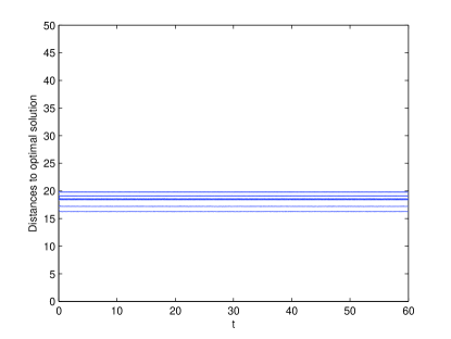
(a) Distance to optimum for sample average scheme with $N$ samples.

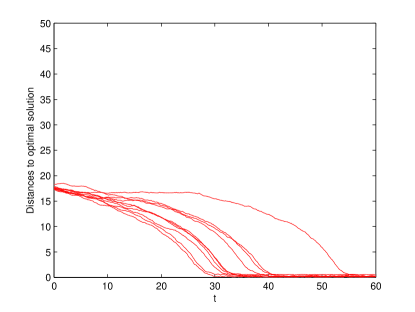
(b) Distance to optimum with flocking discipline.

Figure 2: Performance comparison for Ackley’s function (Case 1).

5.1.2 Ackley’s Function (Case 2)

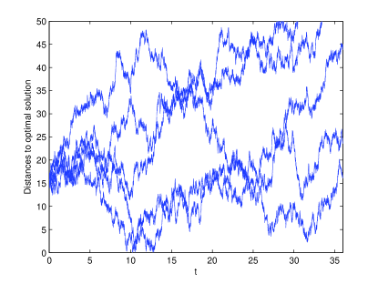
(a) Distance to optimum for sample average scheme with $N$ samples.

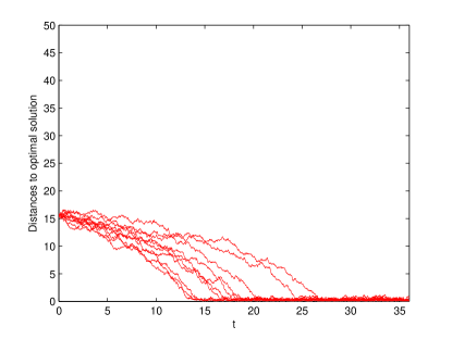
(b) Distance to optimum with flocking discipline.

Figure 3: Performance comparison for Ackley’s function (Case 2).

In this case we assume that the noise level is $\sigma=35$. We use $N=30$ computing threads, and the attraction/repulsion function $g(x)=-x[3-0.01\exp(-\|x\|^{2})]$ is adopted. In the flocking-based approach, each thread randomly communicates with 8 other threads. Overhead parameter $\beta=1.5$. Sampling times are constant with $\tilde{\Delta}t=0.04$ and $\Delta t=N^{{1}/{\beta}}\tilde{\Delta}t\simeq 0.184$, respectively. Step sizes are $\tilde{\Gamma}=0.04$ and $\Gamma=0.184$. Initially, the sampling points were distributed randomly in the $[10,12]\times[10,12]$ interval. Simulations run for 36s.

We can see in Figure 3(a) that individual threads operating in parallel are not able to approach the globally optimal solution. On the contrary, the flocking discipline allows convergence to the global optimum successfully (see Figure 3(b)).

5.2 Asymptotic Noise Reduction

We now discuss the asymptotic noise reduction properties of the flocking-based algorithmic scheme for non-convex optimization. We start by reviewing the asymptotic performance of the centralized algorithm based upon the average of $N$ samples per step. Recalling (4),

$$dy_{t}=-\nabla f(y_{t})\gamma dt+\tau_{N}\gamma dB_{t},$$

The limiting density of $y_{t}$ (which solves a related Fokker-Planck equation (see [3, risken1984fokker])) is

$$\hat{\pi}(y_{t})=\frac{\exp\{-2f(x)/(\tau_{N}^{2}\gamma)\}}{\int\exp\{-2f(y)/(\tau_{N}^{2}\gamma)\}}=\frac{\exp\{-2Nf(y)/(\sigma^{2}\tilde{\Gamma})\}}{\int\exp\{-2Nf(y)/(\sigma^{2}\tilde{\Gamma})\}}$$

assuming $\Gamma=\tilde{\Gamma}$.

We return now to the flocking scheme. By equation (6) and the relation $g(x)=-\nabla_{x}J(\|x\|)$, we have

$$dy_{i,t}=\left[-\nabla f(y_{i,t})-\sum_{j=1,j\neq i}^{N}\alpha_{ij}\nabla_{y_{i,t}}J\|y_{i,t}-y_{j,t}\|\right]\tilde{\gamma}dt+\tau\tilde{\gamma}dB_{i,t}.$$ (20)

Let $\mathbf{y}_{t}=[y_{1,t}^{T},\ldots,y_{N,t}^{T}]^{T}\in\mathbb{R}^{N\times m}$, $\mathbf{B_{t}}=[B_{1,t}^{T},\ldots,B_{N,t}^{T}]^{T}\in\mathbb{R}^{N\times m}$. Define

$$H(\mathbf{y}_{t})=\sum_{i=1}^{N}f(y_{i,t})+\frac{1}{2}\sum_{i=1}^{N}\sum_{j=1,j\neq i}^{N}\alpha_{ij}J(\|y_{i,t}-y_{j,t}\|).$$ (21)

We can rewrite (20) in a compact form:

$$d\mathbf{y}_{t}=-\nabla H(\mathbf{y}_{t})\tilde{\gamma}dt+\tau\tilde{\gamma}d\mathbf{B}_{t}.$$ (22)

The Fokker-Planck equation related to the stochastic differential equation (22) is:

$$\frac{\partial p_{t}}{\partial t}=-\nabla\cdot(\nabla H(\mathbf{y})\tilde{\gamma}p_{t})+\frac{\tau^{2}\tilde{\gamma}^{2}}{2}\nabla^{2}p_{t}$$ (23)

where $p_{t}:=p(\mathbf{y}_{t},t\mid\mathbf{y}_{0},0)$ is the probability density of $\mathbf{y}_{t}$.

Proposition 2.

Suppose relation (6) holds, and $\int\exp\{-2H(\mathbf{y})/\tau^{2}\}d\mathbf{y}$ is finite. Then $\mathbf{y}_{t}$ weakly approaches a unique equilibrium, which is a Gibbs distribution with density

$$\pi(\mathbf{y})=\frac{1}{K}\exp\{-2H(\mathbf{y})/(\tau^{2}\tilde{\gamma})\},$$ (24)

where

$$K=\int\exp\{-2H(\mathbf{y})/(\tau^{2}\tilde{\gamma})\}d\mathbf{y}.$$

Proposition 2 comes from the standard theory of diffusion (see [3, risken1984fokker]). The assumption is required for the distribution (24) to be well-defined. It is satisfied when $H(\mathbf{y})$ grows rapidly enough, or when the feasible region $X$ has reflected boundaries.

We now show that for large values of the parameter $a$ (attractive force) the asymptotic noise reduction properties of the flocking-based algorithmic scheme is the same to that of a centralized algorithm based upon the average of $N$ samples per step.

Theorem 3.

Suppose relation (6) holds. Assume linear attraction functions $g_{a}(\|x\|)=a$ for some $a>0$ and repulsion functions satisfying $g_{r}(\|x\|)\|x\|^{2}\leq b$. Then the asymptotic probability distribution of $\overline{y}_{t}$ has density:

$$\pi^{*}(\overline{y})=\frac{\exp\left\{-2Nf(\overline{y})/(\sigma^{2}\tilde{\Gamma})\right\}}{\int\exp\left\{-2Nf(\overline{y})/(\sigma^{2}\tilde{\Gamma})\right\}d\overline{y}},$$

as $a\rightarrow\infty$.

Proof.

See Appendix 7.6. ∎

Remark 6.

The asymptotic probability distribution of $\overline{x}_{t}$ is the same as that of $\overline{y}_{t}$.

Remark 7.

The limiting probability density of $\overline{x}_{t}$ as $a\rightarrow\infty$ does not depend on the specific network topology as long as $\lambda_{2}>0$, i.e., the network is connected. This is a very mild networking requirement satisfied by many simple topologies (e.g. ring, line, bus, mesh).

Remark 8.

As $N\rightarrow\infty$, $\pi^{*}(\overline{x})$ concentrates on the global minima of $f(\cdot)$, in which case the average solution of the flocking scheme is guaranteed to approximate a global minimum (see [7] for a reference).

6 Conclusions

In recent years, the paradigm of cloud computing has emerged as an architecture for computing that makes use of distributed (networked) computing resources. In this paper, we analyze a distributed computing algorithmic scheme for stochastic optimization which relies on modest communication requirements amongst processors and most importantly, does not require synchronization. The proposed distributed algorithmic framework may provide significant speed-up in application domains in which sampling times are non-negligible. This is the case, for example, in the optimization of complex systems for which performance may only be evaluated via computationally intensive Òblack-boxÓ simulation models.

The scheme considered in this paper has $N>1$ computing threads operating under a connected network. At each step, each thread independently computes a new solution by using a noisy estimation of the gradient, which is further perturbed by a combination of repulsive and attractive terms depending upon the relative distance to solutions identified by neighboring threads. When the objective function is convex, we showed that a flocking-like approach for distributed stochastic optimization provides a noise reduction effect similar to that of a centralized stochastic gradient algorithm based upon the average of $N$ gradient samples at each step. When the overhead related to the time needed to gather $N$ samples and synchronization is not negligible, the flocking implementation outperforms a centralized stochastic gradient algorithm based upon the average of $N$ gradient samples at each step. When the objective function is not convex, the flocking-based approach seems better suited to escape locally optimal solutions due to the repulsive force which enforces a certain level of diversity in the set of candidate solutions. Here again, we showed that the noise reduction effect is similar to that associated to the centralized stochastic gradient algorithm based upon the average of $N$ gradient samples at each step.

7 Appendix

7.1 Notations

Table 1: Notations

Symbol	Meaning
$m$	Dimension of the solution space
$N$	Number of computing threads
$\Gamma$ (respectively, $\tilde{\Gamma}$)	Step size for the centralized algorithm (respectively, flocking-based algorithm)
$\Delta t$	Average sampling time to gather $N$ samples in parallel
$\tilde{\Delta}t$	Average sampling time to gather one sample
$\varepsilon(k)$	Simulation noise from one sample (centralized algorithm)
$\varepsilon(i,k)$	Simulation noise from one sample (flocking-based algorithm)
$\sigma$	Variance of $\varepsilon(k)$ and $\varepsilon(i,k)$ (in each dimension)
$\gamma$	$1/\Delta t$
$\tilde{\gamma}$	$1/\tilde{\Delta}t$
$\tau_{N}$	$\sigma\sqrt{\Gamma\Delta t/N}$
$\tau$	$\sigma\sqrt{\tilde{\Gamma}\tilde{\Delta}t}$
$a$	Parameter for linear attraction in the flocking term
$b$	Bound on repulsion in the flocking term
$\mathcal{G}$	Interaction graph of “flocking” threads
$\alpha_{ij}$	Indicator of connectivity between thread $i$ and $j$
$A$	Matrix $[\alpha_{ij}]$
$L$	Laplacian matrix of $A$
$\lambda_{2}$	Second-smallest eigenvalue of $L$ (algebraic connectivity of $\mathcal{G}$)
$\eta$	Bound on the gradient of $f(\cdot)$
$\kappa$	Strong convexity parameter
$\mu$	Lipschitz constant

7.2 Proof of Lemma 2

Since $A=A^{T}$ and $g(\cdot)$ is an odd function,

$$d{\overline{y}_{t}}=\frac{1}{N}\sum_{i=1}^{N}d{y_{i,t}}=\frac{1}{N}\sum_{i=1}^{N}\left[-\nabla f(y_{i,t})\tilde{\gamma}dt+\sum_{j=1,j\neq i}^{N}\alpha_{ij}g(y_{i,t}-y_{j,t})\tilde{\gamma}dt+\tau\tilde{\gamma}dB_{i,t}\right]\\ =-\frac{1}{N}\sum_{i=1}^{N}\nabla f(y_{i,t})\tilde{\gamma}dt+\frac{\tau}{N}\tilde{\gamma}\sum_{i=1}^{N}{dB_{i,t}}.$$ (25)

By (6) and (25),

$$d{e_{i,t}}= d{y}_{i,t}-d{\overline{y}_{t}}$$

$$= \sum_{j=1,j\neq i}^{N}\alpha_{ij}g(y_{i,t}-y_{j,t})\tilde{\gamma}dt-\nabla f(y_{i,t})\tilde{\gamma}dt+\frac{1}{N}\sum_{i=1}^{N}\nabla f({x}_{i,t})\tilde{\gamma}dt+\tau\tilde{\gamma}{dB_{i,t}}-\frac{\tau}{N}\tilde{\gamma}\sum_{i=1}^{N}{dB_{i,t}}.$$ (26)

From equation (7) and the assumption that $g_{a}(\|x\|)=a$,

$$g(y_{i,t}-y_{j,t})=-(y_{i,t}-y_{j,t})[g_{a}(\|y_{i,t}-y_{j,t}\|)-g_{r}(\|y_{i,t}-y_{j,t}\|)]=-(y_{i,t}-y_{j,t})[a-g_{r}(\|y_{i,t}-y_{j,t}\|)].$$

We then have

$$\sum_{j=1,j\neq i}^{N}\alpha_{ij}g(y_{i,t}-y_{j,t})=-a\sum_{j=1,j\neq i}^{N}\alpha_{ij}(y_{i,t}-y_{j,t})+\sum_{j=1,j\neq i}^{N}\alpha_{ij}g_{r}(\|y_{i,t}-y_{j,t}\|)(y_{i,t}-y_{j,t}).$$

Consequently, equation (7.2) becomes

$$d{e_{i,t}}=-a\sum_{j=1,j\neq i}^{N}\alpha_{ij}(y_{i,t}-y_{j,t})\tilde{\gamma}dt+\sum_{j=1,j\neq i}^{N}\alpha_{ij}g_{r}(\|y_{i,t}-y_{j,t}\|)(y_{i,t}-y_{j,t})\tilde{\gamma}dt-\nabla f(y_{i,t})\tilde{\gamma}dt\\ +\frac{1}{N}\sum_{j=1}^{N}\nabla f({x}_{j,t})\tilde{\gamma}dt+\tau\tilde{\gamma}{dB_{i,t}}-\frac{\tau}{N}\tilde{\gamma}\sum_{j=1}^{N}{dB_{j,t}}.$$ (27)

In light of the facts that $dt\cdot dt=dt\cdot dB_{i,t}=0$, $dB_{i,t}\cdot dB_{j,t}=0$ ($i\neq j$), and $dB_{i,t}\cdot dB_{i,t}=mdt$ (see [18]),

$$de_{i,t}\cdot de_{i,t}=\left(1-\frac{1}{N}\right)m\tau^{2}\tilde{\gamma}^{2}dt.$$

Then from Ito’s lemma,

$$d{V_{i,t}}= d{e_{i,t}}\cdot e_{i,t}+\frac{1}{2}de_{i,t}\cdot de_{i,t}$$

$$= -a\sum_{j=1,j\neq i}^{N}\alpha_{ij}(y_{i,t}-y_{j,t})^{T}e_{i,t}\tilde{\gamma}dt+\sum_{j=1,j\neq i}^{N}\alpha_{ij}g_{r}(\|y_{i,t}-y_{j,t}\|)(y_{i,t}-y_{j,t})^{T}e_{i,t}\tilde{\gamma}dt$$

$$-\left[\nabla f(y_{i,t})-\frac{1}{N}\sum_{j=1}^{N}\nabla f({x}_{j,t})\right]^{T}e_{i,t}\tilde{\gamma}dt+\left[\tau\tilde{\gamma}{dB_{i,t}}-\frac{\tau}{N}\tilde{\gamma}\sum_{j=1}^{N}{dB_{j,t}}\right]^{T}e_{i,t}+\frac{m\tau^{2}\tilde{\gamma}^{2}}{2}\left(1-\frac{1}{N}\right)dt.$$ (28)

In conclusion, the stochastic differential equation is

$$d\overline{V}_{t}= \frac{1}{N}\sum_{i=1}^{N}dV_{i,t}$$

$$= -\frac{a}{N}\sum_{i=1}^{N}\sum_{j=1,j\neq i}^{N}\alpha_{ij}(y_{i,t}-y_{j,t})^{T}e_{i,t}\tilde{\gamma}dt+\frac{1}{N}\sum_{i=1}^{N}\sum_{j=1,j\neq i}^{N}\alpha_{ij}g_{r}(\|y_{i,t}-y_{j,t}\|)(y_{i,t}-y_{j,t})^{T}e_{i,t}\tilde{\gamma}dt$$

$$-\frac{1}{N}\sum_{i=1}^{N}\nabla^{T}f(y_{i,t})e_{i,t}\tilde{\gamma}dt+\frac{\tau}{N}\tilde{\gamma}\sum_{i=1}^{N}{dB_{i,t}}^{T}e_{i,t}+\frac{m\tau^{2}\tilde{\gamma}^{2}(N-1)}{2N}dt$$

$$= -\frac{a}{N}\sum_{i=1}^{N}\sum_{j=1,j\neq i}^{N}\alpha_{ij}(e_{i,t}-e_{j,t})^{T}e_{i,t}\tilde{\gamma}dt+\frac{1}{2N}\sum_{i=1}^{N}\sum_{j=1,j\neq i}^{N}\alpha_{ij}g_{r}(\|y_{i,t}-y_{j,t}\|)\|y_{i,t}-y_{j,t}\|^{2}\tilde{\gamma}dt$$

$$-\frac{1}{N}\sum_{i=1}^{N}\nabla^{T}f(y_{i,t})e_{i,t}\tilde{\gamma}dt+\frac{\tau}{N}\tilde{\gamma}\sum_{i=1}^{N}{dB_{i,t}}^{T}e_{i,t}+\frac{m\tau^{2}\tilde{\gamma}^{2}(N-1)}{2N}dt.$$

7.3 Proof of Theorem 1

7.3.1 Case 1

By equation (2),

$$d\overline{V}_{t}= -\frac{a}{N}\sum_{i=1}^{N}\sum_{j=1,j\neq i}^{N}\alpha_{ij}(e_{i,t}-e_{j,t})^{T}e_{i,t}\tilde{\gamma}dt+\frac{1}{2N}\sum_{i=1}^{N}\sum_{j=1,j\neq i}^{N}\alpha_{ij}g_{r}(\|y_{i,t}-y_{j,t}\|)\|y_{i,t}-y_{j,t}\|^{2}\tilde{\gamma}dt$$

$$-\frac{1}{N}\sum_{i=1}^{N}\nabla^{T}f(y_{i,t})e_{i,t}\tilde{\gamma}dt+\frac{\tau}{N}\tilde{\gamma}\sum_{i=1}^{N}{dB_{i,t}}^{T}e_{i,t}+\frac{m\tau^{2}\tilde{\gamma}^{2}(N-1)}{2N}dt.$$

Noticing that $g_{r}(\|y_{i,t}-y_{j,t}\|)\|y_{i,t}-y_{j,t}\|^{2}\leq b$, by (9) and (10),

$$d\overline{V}_{t}\leq -2{a}\lambda_{2}\tilde{\gamma}\overline{V}_{t}dt+\frac{b|Tr(L)|}{2N}\tilde{\gamma}dt+\frac{m\tau^{2}\tilde{\gamma}^{2}(N-1)}{2N}dt+\frac{1}{N}\sum_{i=1}^{N}\eta\|e_{i,t}\|\tilde{\gamma}dt+\frac{\tau}{N}\tilde{\gamma}\sum_{i=1}^{N}{dB_{i,t}}^{T}e_{i,t}$$

$$\leq -2{a}\lambda_{2}\tilde{\gamma}\overline{V}_{t}dt+\left[\frac{b|Tr(L)|}{2N}\tilde{\gamma}+\frac{m\tau^{2}\tilde{\gamma}^{2}(N-1)}{2N}\right]dt+\sqrt{2}{\eta}\sqrt{\overline{V}_{t}}\tilde{\gamma}dt+\frac{\tau}{N}\tilde{\gamma}\sum_{i=1}^{N}{dB_{i,t}}^{T}e_{i,t}$$

$$\leq -c_{1}\tilde{\gamma}\overline{V}_{t}dt-(2a\lambda_{2}-c_{1})\tilde{\gamma}\overline{V}_{t}dt+\sqrt{2}{\eta}\sqrt{\overline{V}_{t}}\tilde{\gamma}dt+\left[\frac{b|Tr(L)|}{2N}\tilde{\gamma}+\frac{m\tau^{2}\tilde{\gamma}^{2}(N-1)}{2N}\right]dt$$

$$+\frac{\tau}{N}\tilde{\gamma}\sum_{i=1}^{N}{dB_{i,t}}^{T}e_{i,t}$$

$$= -c_{1}\tilde{\gamma}\overline{V}_{t}dt-(2a\lambda_{2}-c_{1})\left[\sqrt{\overline{V}}-\frac{\sqrt{2}{\eta}}{2(2a\lambda_{2}-c_{1})}\right]^{2}\tilde{\gamma}dt$$

$$+\left[\frac{\eta^{2}}{2(2a\lambda_{2}-c_{1})}\tilde{\gamma}+\frac{b|Tr(L)|}{2N}\tilde{\gamma}+\frac{m\tau^{2}\tilde{\gamma}^{2}(N-1)}{2N}\right]dt+\frac{\tau}{N}\tilde{\gamma}\sum_{i=1}^{N}{dB_{i,t}}^{T}e_{i,t}$$

$$\leq -c_{1}\tilde{\gamma}\overline{V}_{t}dt+c_{2}\tilde{\gamma}dt+\frac{\tau}{N}\tilde{\gamma}\sum_{i=1}^{N}{dB_{i,t}}^{T}e_{i,t},$$

where $c_{1}\in\left(0,2a\lambda_{2}\right)$ is arbitrary, and

$$c_{2}=\frac{\eta^{2}}{2(2a\lambda_{2}-c_{1})}+\frac{b|Tr(L)|}{2N}+\frac{m\tau^{2}\tilde{\gamma}(N-1)}{2N}.$$

Applying Ito’s lemma to $e^{c_{1}\tilde{\gamma}t}\overline{V}_{t}$,

$$d(e^{c_{1}\tilde{\gamma}t}\overline{V}_{t})=e^{c_{1}\tilde{\gamma}t}d\overline{V}_{t}+c_{1}\tilde{\gamma}e^{c_{1}\tilde{\gamma}t}\overline{V}_{t}dt\leq c_{2}\tilde{\gamma}e^{c_{1}\tilde{\gamma}t}dt+\frac{\tau}{N}\tilde{\gamma}e^{c_{1}\tilde{\gamma}t}\sum_{i=1}^{N}{dB_{i,t}}^{T}e_{i,t}.$$

Integrating the stochastic differential inequality,

$$\overline{V}_{t}\leq e^{-c_{1}\tilde{\gamma}t}\overline{V}_{0}+\frac{c_{2}}{c_{1}}(1-e^{-c_{1}\tilde{\gamma}t})+e^{-c_{1}\tilde{\gamma}t}\int_{0}^{t}\frac{\tau}{N}\tilde{\gamma}e^{c_{1}\tilde{\gamma}s}\sum_{i=1}^{N}{dB_{i,s}}^{T}e_{i,s}.$$

Taking an ensemble average on both sides yields

$$\mathbb{E}[\overline{V}_{t}]\leq e^{-c_{1}\tilde{\gamma}t}\overline{V}_{0}+\frac{c_{2}}{c_{1}}(1-e^{-c_{1}\tilde{\gamma}t}).$$ (29)

It follows that

$$\mathbb{E}[\overline{V}_{t}]\leq(\overline{V}_{0}-\frac{c_{2}}{c_{1}})e^{-c_{1}\tilde{\gamma}t}+\frac{c_{2}}{c_{1}}\leq\left\{\begin{array}[]{lcc}\overline{V}_{0}&\text{if}\ \ \overline{V}_{0}\geq\cfrac{c_{2}}{c_{1}},&\\ \cfrac{c_{2}}{c_{1}}&\text{if}\ \ \overline{V}_{0}<\cfrac{c_{2}}{c_{1}}.&\end{array}\right.$$

Therefore

$$\mathbb{E}[\overline{V}_{t}]\leq\max\{\overline{V}_{0},\frac{c_{2}}{c_{1}}\},\forall t,$$ (30)

In the long run,

$$\mathbb{E}[\overline{V}_{t}]\leq\frac{c_{2}}{c_{1}}=\frac{\eta^{2}}{2c_{1}(2a\lambda_{2}-c_{1})}+\frac{b|Tr(L)|}{2c_{1}N}+\frac{m\tau^{2}\tilde{\gamma}(N-1)}{2c_{1}N}.$$ (31)

Notice that the above inequality is valid for all $c_{1}\in(0,2a\lambda_{2})$, of which we look for the minimum over all possible $c_{1}$’s. Define

$$\psi_{1}(c_{1})=\frac{\eta^{2}}{2c_{1}(2a\lambda_{2}-c_{1})}+\frac{b|Tr(L)|}{2c_{1}N}+\frac{m\tau^{2}\tilde{\gamma}(N-1)}{2c_{1}N}\\ =\left[\frac{\eta^{2}}{4a\lambda_{2}}+\frac{b|Tr(L)|}{2N}+\frac{m\tau^{2}\tilde{\gamma}(N-1)}{2N}\right]\frac{1}{c_{1}}+\frac{\eta^{2}}{4a\lambda_{2}}\frac{1}{(2a\lambda_{2}-c_{1})}.$$

By Cauchy-Schwartz inequality, when

$$\frac{1}{c_{1}}=\frac{1}{2a\lambda_{2}}\left(1+\sqrt{\frac{c_{4}}{c_{3}}}\right),$$

$\psi_{1}(c_{1})$ attains its minimum

$$\psi_{1}^{*}=\frac{1}{2a\lambda_{2}}{\left(\sqrt{c_{3}}+\sqrt{c_{4}}\right)^{2}}.$$

Here

$$c_{3}=\frac{\eta^{2}}{4a\lambda_{2}}+\frac{b|Tr(L)|}{2N}+\frac{m\tau^{2}\tilde{\gamma}(N-1)}{2N},c_{4}=\frac{\eta^{2}}{4a\lambda_{2}}.$$

Since (31) is valid for all $c_{1}\in(0,2a\lambda_{2})$, it holds true that $\mathbb{E}[\overline{V}_{t}]\leq\psi_{1}^{*}$ in the long run.

7.3.2 Case 2

Notice that

$$\sum_{i=1}^{N}\nabla^{T}f(y_{i,t})e_{i,t}=\sum_{i=1}^{N}(\nabla^{T}f(y_{i,t})-\nabla^{T}f(\overline{x}_{t}))(y_{i,t}-\overline{x}_{t})\geq\sum_{i=1}^{N}\kappa\|y_{i,t}-\overline{x}_{t}\|^{2}=2\kappa N\overline{V}_{t},$$

where the inequality follows from Assumption 2, and that $g_{r}(\|y_{i,t}-y_{j,t}\|)\|y_{i,t}-y_{j,t}\|^{2}\leq b$. In light of (9) and (10), equation (2) gives

$$d\overline{V}_{t}\leq-2{a}\lambda_{2}\tilde{\gamma}\overline{V}_{t}dt-2\kappa\tilde{\gamma}\overline{V}_{t}dt+\frac{b|Tr(L)|}{2N}\tilde{\gamma}dt+\frac{m\tau^{2}\tilde{\gamma}^{2}(N-1)}{2N}dt+\frac{\tau}{N}\tilde{\gamma}\sum_{i=1}^{N}{dB_{i,t}}^{T}e_{i,t}.$$

By Ito’s lemma,

$$d\left[e^{2(\kappa+a\lambda_{2})\tilde{\gamma}t}\overline{V}_{t}\right] =e^{2(\kappa+a\lambda_{2})\tilde{\gamma}t}d\overline{V}_{t}+2(\kappa+a\lambda_{2})\tilde{\gamma}e^{2(\kappa+a\lambda_{2})\tilde{\gamma}t}\overline{V}_{t}dt$$

$$\leq\left[\frac{b|Tr(L)|}{2N}\tilde{\gamma}dt+\frac{m\tau^{2}\tilde{\gamma}^{2}(N-1)}{2N}\right]e^{2(\kappa+a\lambda_{2})\tilde{\gamma}t}dt+\frac{\tau}{N}\tilde{\gamma}e^{2(\kappa+a\lambda_{2})\tilde{\gamma}t}\sum_{i=1}^{N}{dB_{i,t}}^{T}e_{i,t}.$$

Integrating both sides,

$$\overline{V}_{t}\leq e^{-2(\kappa+a\lambda_{2})\tilde{\gamma}t}\overline{V}_{0}+\left[\frac{b|Tr(L)|}{4N(\kappa+a\lambda_{2})}+\frac{m\tau^{2}\tilde{\gamma}(N-1)}{4N(\kappa+a\lambda_{2})}\right]\left[1-e^{-2(\kappa+a\lambda_{2})\tilde{\gamma}t}\right]\\ +e^{-2(\kappa+a\lambda_{2})\tilde{\gamma}t}\int\limits_{0}^{t}\frac{\tau}{N}\tilde{\gamma}e^{2(\kappa+a\lambda_{2})\tilde{\gamma}s}\sum_{i=1}^{N}{dB_{i,s}^{T}}e_{i,s}.$$

Taking ensemble average yields

$$\mathbb{E}[\overline{V}_{t}]\leq e^{-2(\kappa+a\lambda_{2})\tilde{\gamma}t}\overline{V}_{0}+\left[\frac{b|Tr(L)|}{4N(\kappa+a\lambda_{2})}+\frac{m\tau^{2}\tilde{\gamma}(N-1)}{4N(\kappa+a\lambda_{2})}\right]\left[1-e^{-2(\kappa+a\lambda_{2})\tilde{\gamma}t}\right].$$

In the long run,

$$\mathbb{E}[\overline{V}_{t}]\leq\psi_{2}^{*}=\frac{b|Tr(L)|}{4N(\kappa+a\lambda_{2})}+\frac{m\tau^{2}\tilde{\gamma}(N-1)}{4N(\kappa+a\lambda_{2})}.$$

7.4 Proof of Lemma 3

7.4.1 Preliminaries

According to equation (25) and Ito’s lemma,

$$d{U}_{t}= d({\overline{y}_{t}-x^{\ast}})\cdot(\overline{y}_{t}-x^{\ast})+\frac{1}{2}d(\overline{y}_{t}-x^{\ast})\cdot d(\overline{y}_{t}-x^{\ast})$$

$$= -\frac{1}{N}\sum_{i=1}^{N}\nabla^{T}f(y_{i,t})(\overline{y}_{t}-x^{\ast})\tilde{\gamma}dt+\frac{\tau}{N}\tilde{\gamma}\sum_{i=1}^{N}{dB_{i,t}}^{T}(\overline{y}_{t}-x^{\ast})+\frac{m\tau^{2}\tilde{\gamma}^{2}}{2N}dt$$

$$= -\frac{1}{N}\sum_{i=1}^{N}\nabla^{T}f(y_{i,t})(y_{i,t}-x^{\ast})\tilde{\gamma}dt+\frac{1}{N}\sum_{i=1}^{N}\nabla^{T}f(y_{i,t})e_{i,t}\tilde{\gamma}dt+\frac{\tau}{N}\tilde{\gamma}\sum_{i=1}^{N}{dB_{i,t}}^{T}(\overline{y}_{t}-x^{\ast})+\frac{m\tau^{2}\tilde{\gamma}^{2}}{2N}dt.$$ (32)

Since $f(\cdot)$ attains its minimum at $x^{\ast}$, $\nabla f(x^{\ast})=0$. Then by Assumption 2 and equation (4),

$$-\frac{1}{N}\sum_{i=1}^{N}\nabla^{T}f(y_{i,t})(y_{i,t}-x^{\ast})= -\frac{1}{N}\sum_{i=1}^{N}(\nabla^{T}f(y_{i,t})-\nabla^{T}f(x^{\ast}))(y_{i,t}-x^{\ast})$$

$$\leq -2\kappa\overline{F}_{t}=-2\kappa(U_{t}+\overline{V}_{t}).$$

By Assumption 3,

$$\frac{1}{N}\sum_{i=1}^{N}\nabla^{T}f(y_{i,t})e_{i,t}=\frac{1}{N}\sum_{i=1}^{N}\left(\nabla^{T}f(y_{i,t})-\nabla^{T}f(\overline{x}_{t})\right)(y_{i,t}-\overline{x}_{t})\leq\frac{1}{N}\sum_{i=1}^{N}\mu\|e_{i,t}\|^{2}=2\mu\overline{V}_{t}.$$

Therefore,

$$dU_{t} \leq-2\kappa\tilde{\gamma}(U_{t}+\overline{V}_{t})dt+2\mu\tilde{\gamma}\overline{V}_{t}dt+\frac{m\tau^{2}\tilde{\gamma}^{2}}{2N}dt+\frac{\tau}{N}\tilde{\gamma}\sum_{i=1}^{N}{dB_{i,t}}^{T}\overline{x}_{t}$$

$$=-2\kappa\tilde{\gamma}U_{t}dt+2(\mu-\kappa)\tilde{\gamma}\overline{V}_{t}dt+\frac{m\tau^{2}\tilde{\gamma}^{2}}{2N}dt+\frac{\tau}{N}\tilde{\gamma}\sum_{i=1}^{N}{dB_{i,t}}^{T}\overline{x}_{t}.$$ (33)

By equation (12),

$$d\overline{V}_{t}=-\frac{a}{N}\sum_{i=1}^{N}\sum_{j=1,j\neq i}^{N}\alpha_{ij}(e_{i,t}-e_{j,t})^{T}e_{i,t}\tilde{\gamma}dt-\frac{1}{N}\sum_{i=1}^{N}\nabla^{T}f(y_{i,t})e_{i,t}\tilde{\gamma}dt+\frac{\tau}{N}\tilde{\gamma}\sum_{i=1}^{N}{dB_{i,t}}^{T}e_{i,t}\\ +\frac{m\tau^{2}\tilde{\gamma}^{2}(N-1)}{2N}dt.$$ (34)

Notice that

$$\sum_{i=1}^{N}\nabla^{T}f(y_{i,t})e_{i,t}=\sum_{i=1}^{N}(\nabla^{T}f(y_{i,t})-\nabla^{T}f(\overline{x}_{t}))(y_{i,t}-\overline{x}_{t})\geq\sum_{i=1}^{N}\kappa\|y_{i,t}-\overline{x}_{t}\|^{2}=2\kappa N\overline{V}_{t},$$

where the inequality follows from Assumption 2. In light of (9) and (10),

$$d\overline{V}_{t}\leq-2{a}\lambda_{2}\tilde{\gamma}\overline{V}_{t}dt-2\kappa\tilde{\gamma}\overline{V}_{t}dt+\frac{m\tau^{2}\tilde{\gamma}^{2}(N-1)}{2N}dt+\frac{\tau}{N}\tilde{\gamma}\sum_{i=1}^{N}{dB_{i,t}}^{T}e_{i,t}.$$ (35)

7.4.2 Proof of Lemma 3

Define

$$W_{t}=U_{t}+\frac{(\mu-\kappa)}{a\lambda_{2}}\overline{V}_{t}.$$ (36)

By (7.4.1) and (35),

$$dW_{t}\leq -2\kappa\tilde{\gamma}U_{t}dt+\left[2(\mu-\kappa)-\frac{(\mu-\kappa)}{a\lambda_{2}}(2\kappa+2a\lambda_{2})\right]\tilde{\gamma}\overline{V}_{t}dt+\frac{m\tau^{2}\tilde{\gamma}^{2}}{2N}dt+\frac{m\tau^{2}\tilde{\gamma}^{2}(\mu-\kappa)(N-1)}{2aN\lambda_{2}}dt$$

$$+\frac{\tau}{N}\tilde{\gamma}\sum_{i=1}^{N}{dB_{i,t}}^{T}\overline{x}_{t}+\frac{\tau(\mu-\kappa)}{aN\lambda_{2}}\tilde{\gamma}\sum_{i=1}^{N}{dB_{i,t}}^{T}e_{i,t}$$

$$= -2\kappa\tilde{\gamma}W_{t}dt+\frac{m\tau^{2}\tilde{\gamma}^{2}}{2N}\left[1+\frac{(\mu-\kappa)(N-1)}{a\lambda_{2}}\right]dt+\frac{\tau}{N}\tilde{\gamma}\sum_{i=1}^{N}{dB_{i,t}}^{T}\overline{x}_{t}+\frac{\tau(\mu-\kappa)}{aN\lambda_{2}}\tilde{\gamma}\sum_{i=1}^{N}{dB_{i,t}}^{T}e_{i,t}.$$

Then,

$$d(e^{2\kappa\tilde{\gamma}t}W_{t}) =e^{2\kappa\tilde{\gamma}t}dW_{t}+2\kappa\tilde{\gamma}e^{2\kappa\tilde{\gamma}t}W_{t}dt$$

$$\leq\frac{m\tau^{2}\tilde{\gamma}^{2}}{2N}\left[1+\frac{(\mu-\kappa)(N-1)}{a\lambda_{2}}\right]e^{2\kappa\tilde{\gamma}t}dt+\frac{\tau}{N}\tilde{\gamma}e^{2\kappa\tilde{\gamma}t}\left[\sum_{i=1}^{N}{dB_{i,t}}^{T}\overline{x}_{t}+\frac{(\mu-\kappa)}{a\lambda_{2}}\sum_{i=1}^{N}{dB_{i,t}}^{T}e_{i,t}\right].$$

Integrating both sides yields

$$W_{t}\leq e^{-2\kappa\tilde{\gamma}t}W_{0}+\frac{m\tau^{2}\tilde{\gamma}}{4\kappa N}\left[1+\frac{(\mu-\kappa)(N-1)}{a\lambda_{2}}\right](1-e^{-2\kappa\tilde{\gamma}t})\\ +e^{-2\kappa\tilde{\gamma}t}\int_{0}^{t}\frac{\tau}{N}\tilde{\gamma}e^{2\kappa\tilde{\gamma}s}\left[\sum_{i=1}^{N}{dB_{i,s}}^{T}\overline{x}_{s}+\frac{(\mu-\kappa)}{a\lambda_{2}}\sum_{i=1}^{N}{dB_{i,s}}^{T}e_{i,s}\right].$$

Taking ensemble average, we get

$$\mathbb{E}[W_{t}]\leq e^{-2\kappa\tilde{\gamma}t}W_{0}+\frac{m\tau^{2}\tilde{\gamma}}{4\kappa N}\left[1+\frac{(\mu-\kappa)(N-1)}{a\lambda_{2}}\right](1-e^{-2\kappa\tilde{\gamma}t}).$$

By (36),

$$\mathbb{E}[U_{t}]\leq\mathbb{E}[W_{t}]\leq e^{-2\kappa\tilde{\gamma}t}\left[U_{0}+\frac{(\mu-\kappa)}{a\lambda_{2}}\overline{V}_{0}\right]+\frac{m\tau^{2}\tilde{\gamma}}{4\kappa N}\left[1+\frac{(\mu-\kappa)(N-1)}{a\lambda_{2}}\right](1-e^{-2\kappa\tilde{\gamma}t}).$$

In the long run,

$$\mathbb{E}[U_{t}]\leq\frac{m\tau^{2}\tilde{\gamma}}{4\kappa N}\left[1+\frac{(\mu-\kappa)(N-1)}{a\lambda_{2}}\right].$$ (37)

7.5 Proof of Proposition 1

By (14) and (18),

$$\frac{1}{2}\mathbb{E}[\|x_{t}-x^{\ast}\|^{2}]\geq e^{-2\mu\gamma\Gamma t}G_{0}+\frac{m\tau_{N}^{2}\gamma}{4\mu}(1-e^{-2\mu\gamma\Gamma t}),$$

and

$$\frac{1}{2}\mathbb{E}[\|\bar{x}_{t}-x^{\ast}\|^{2}]\leq e^{-2\kappa\tilde{\gamma}\tilde{\Gamma}t}\left[U_{0}+\frac{(\mu-\kappa)}{a\lambda_{2}}\overline{V}_{0}\right]+\frac{m\tau^{2}\tilde{\gamma}}{4\kappa N}\left[1+\frac{(\mu-\kappa)(N-1)}{a\lambda_{2}}\right](1-e^{-2\kappa\tilde{\gamma}\tilde{\Gamma}t}).$$

Let

$$d_{1}=\frac{m\tau_{N}^{2}\gamma}{4\mu},\ \ d_{2}=U_{0}+\frac{(\mu-\kappa)}{a\lambda_{2}}\overline{V}_{0},$$

and

$$d_{3}=\frac{m\tau^{2}\tilde{\gamma}}{4\kappa N}\left[1+\frac{(\mu-\kappa)(N-1)}{a\lambda_{2}}\right].$$

It follows that

$$\mathbb{E}[\|x_{t}-x^{\ast}\|^{2}]\geq 2(G_{0}-d_{1})e^{-2\mu\gamma\Gamma t}+2d_{1},$$

and

$$\mathbb{E}[\|\bar{x}_{t}-x^{\ast}\|^{2}]\leq 2(d_{2}-d_{3})e^{-2\kappa\tilde{\gamma}\tilde{\Gamma}t}+2d_{3}.$$

From the discussion in Section 4.1, $d_{1}\sim 1/N^{(1/\beta)-1}$ and $d_{3}\sim 1/N$. Therefore, there exists $N^{*}$ such that when $N>N^{*}$, $d_{3}<d_{1}$. In this case, let $t^{*}$ be such that

$$d_{1}-d_{3}=|G_{0}-d_{1}|e^{-2\mu\gamma\Gamma t^{*}}+|d_{2}-d_{3}|e^{-2\kappa\tilde{\gamma}\tilde{\Gamma}t^{*}}.$$

Then for all $t>t^{*}$,

$$\mathbb{E}[\|\bar{x}_{t}-x^{\ast}\|^{2}]<\mathbb{E}[\|x_{t}-x^{\ast}\|^{2}].$$

7.6 Proof of Theorem 3

We start by looking for the joint density of $(\overline{y}^{T},e_{1}^{T},\dots,e_{N-1}^{T})$. Notice that $(\overline{y}^{T},e_{1}^{T},\dots,e_{N-1}^{T})=(D\otimes I_{m})\mathbf{y}_{t}$, where $D$ is a $N\times N$ matrix. It is easy to verify that $D$ has full rank, so that $(D\otimes I_{m})^{-1}$ exists. It follows that (see [13])

$$\pi(\overline{y}^{T},e_{1}^{T},\dots,e_{N-1}^{T}) =\frac{1}{\det(D\otimes I_{m})}\pi((D\otimes I_{m})^{-1}(\overline{y}^{T},e_{1}^{T},\dots,e_{N-1}^{T}))$$

$$=\frac{1}{\tilde{K}}\exp\left\{-2\left[\sum_{i=1}^{N}f(\overline{y}+e_{i})+\frac{1}{2}\sum_{i=1}^{N}\sum_{j=1,j\neq i}^{N}\alpha_{ij}J(\|e_{i,t}-e_{j,t}\|)\right]/(\tau^{2}\tilde{\gamma})\right\}.$$

where $\tilde{K}$ is a normalizing factor. The density of $\overline{y}$ is calculated as

$$\pi(\overline{y})=\frac{1}{\tilde{K}}\int\exp\left\{-2\left[\sum_{i=1}^{N}f(\overline{y}+e_{i})+\frac{1}{2}\sum_{i=1}^{N}\sum_{j=1,j\neq i}^{N}\alpha_{ij}J(\|e_{i,t}-e_{j,t}\|)\right]/(\tau^{2}\tilde{\gamma})\right\}de_{1}\cdots de_{N-1}.$$

Notice that $e_{N}=-\sum_{i=1}^{N-1}e_{i}$ in the equation above. We rewrite the potential function $J$ as a sum of two parts: $J=J_{a}+J_{r}$, where $\nabla_{x}J_{a}(\|x\|)=xg_{a}(\|x\|)=ax$, and $\nabla_{x}J_{r}(\|x\|)=xg_{r}(\|x\|)$. Without loss of generality, we assume that $J_{a}(\|x\|)=({1}/{2})a\|x\|^{2}$. Then (refer to Godsil and Royle [8])

$$\pi(\overline{y}) =\frac{1}{\tilde{K}}\int\exp\left\{-2\left[\sum_{i=1}^{N}f(\overline{y}+e_{i})+\frac{1}{2}\sum_{i=1}^{N}\sum_{j=1,j\neq i}^{N}\alpha_{ij}\frac{a}{2}\|e_{i}-e_{j}\|^{2}+R\right]/(\tau^{2}\tilde{\gamma})\right\}de_{1}\cdots de_{N-1}$$

$$=\frac{1}{\tilde{K}}\int\exp\left\{-2\left[\sum_{i=1}^{N}f(\overline{y}+e_{i})+\frac{a}{2}\mathbf{e}^{T}(L\otimes I_{m})\mathbf{e}+R\right]/(\tau^{2}\tilde{\gamma})\right\}de_{1}\cdots de_{N-1},$$

where

$$R=\frac{1}{2}\sum_{i=1}^{N}\sum_{j=1,j\neq i}^{N}\alpha_{ij}J_{r}(\|e_{i,t}-e_{j,t}\|).$$

Let $z_{i}=a^{{1}/{2}}e_{i},\forall i$.

$$\int\exp\left\{-2\left[\sum_{i=1}^{N}f(\overline{y}+e_{i})+\frac{a}{2}\mathbf{e}^{T}(L\otimes I_{m})\mathbf{e}+R\right]/(\tau^{2}\tilde{\gamma})\right\}de_{1}\cdots de_{N-1}\\ =a^{-(N-1)/2}\int\exp\left\{-2\left[\sum_{i=1}^{N}f(\overline{y}+a^{-{1}/{2}}z_{i})+\frac{1}{2}\mathbf{z}^{T}(L\otimes I_{m})\mathbf{z}+\tilde{R}\right]/(\tau^{2}\tilde{\gamma})\right\}dz_{1}\cdots dz_{N-1}.$$

Here

$$\tilde{R}=\frac{1}{2}\sum_{i=1}^{N}\sum_{j=1,j\neq i}^{N}\alpha_{ij}J_{r}(a^{-1/2}\|z_{i,t}-z_{j,t}\|).$$

Given that graph $\mathcal{G}$ is connected, $\mathbf{z}^{T}(L\otimes I_{m})\mathbf{z}\geq\lambda_{2}\mathbf{e}^{T}\mathbf{e}$ with $\lambda_{2}>0$. Then since $f$ and $J_{r}$ are continuous, we have

$$\lim\limits_{a\rightarrow\infty}\int\exp\left\{-2\left[\sum_{i=1}^{N}f(\overline{y}+a^{-{1}/{2}}z_{i})+\frac{1}{2}\mathbf{z}^{T}(L\otimes I_{m})\mathbf{z}+\tilde{R}\right]/(\tau^{2}\tilde{\gamma})\right\}dz_{1}\cdots dz_{N-1}\\ =\int\exp\left\{-2\left[Nf(\overline{y})+\frac{1}{2}\mathbf{z}^{T}(L\otimes I_{m})\mathbf{z}+\tilde{R}_{0}\right]/(\tau^{2}\tilde{\gamma})\right\}dz_{1}\cdots dz_{N-1}\\ =\exp\{-2Nf(\overline{y})/(\tau^{2}\tilde{\gamma})\}\exp\{-2\tilde{R}_{0}/(\tau^{2}\tilde{\gamma})\}\int\exp\left\{\mathbf{z}^{T}(L\otimes I_{m})\mathbf{z}/(\tau^{2}\tilde{\gamma})\right\}dz_{1}\cdots dz_{N-1},$$

where

$$\tilde{R}_{0}=\frac{1}{2}\sum_{i=1}^{N}\sum_{j=1,j\neq i}^{N}\alpha_{ij}J_{r}(0)=\frac{1}{2}|Tr(L)|J_{r}(0).$$

Therefore,

$$\lim\limits_{a\rightarrow\infty}\pi(\overline{y})$$

$$=\lim\limits_{a\rightarrow\infty}\frac{1}{\tilde{K}}\int\exp\left\{-2\left[\sum_{i=1}^{N}f(\overline{y}+e_{i})+\frac{1}{2}\sum_{i=1}^{N}\sum_{j=1,j\neq i}^{N}\alpha_{ij}J(\|e_{i,t}-e_{j,t}\|)\right]/(\tau^{2}\tilde{\gamma})\right\}de_{1}\cdots de_{N-1}$$

$$=\frac{\exp\{-2Nf(\overline{y})/(\tau^{2}\tilde{\gamma})\}\exp\{-2\tilde{R}_{0}/\tau^{2}\}\int\exp\left\{\mathbf{z}^{T}(L\otimes I_{m})\mathbf{z}/(\tau^{2}\tilde{\gamma})\right\}dz_{1}\cdots dz_{N-1}}{\int\exp\{-2Nf(\overline{y})/(\tau^{2}\tilde{\gamma})\}\exp\{-2\tilde{R}_{0}/(\tau^{2}\tilde{\gamma})\}\int\exp\left\{\mathbf{z}^{T}(L\otimes I_{m})\mathbf{z}/(\tau^{2}\tilde{\gamma})\right\}dz_{1}\cdots dz_{N-1}d\overline{y}}$$

$$=\frac{\exp\{-2Nf(\overline{y})/(\tau^{2}\tilde{\gamma})\}}{\int\exp\{-2Nf(\overline{y})/(\tau^{2}\tilde{\gamma})\}d\overline{y}}$$

$$=\frac{\exp\left\{-2Nf(\overline{y})/(\sigma^{2}\tilde{\Gamma})\right\}}{\int\exp\left\{-2Nf(\overline{y})/(\sigma^{2}\tilde{\Gamma})\right\}d\overline{y}}.$$

This completes the proof.

References

- [1] Renato LG Cavalcante and Sławomir Stanczak. A distributed subgradient method for dynamic convex optimization problems under noisy information exchange. IEEE Journal of Selected Topics in Signal Processing, 7(2):243–256, 2013.
- [2] Michael C Fu. Stochastic gradient estimation. In Handbook of simulation optimization, pages 105–147. Springer, 2015.
- [3] Crispin W Gardiner. Handbook of stochastic methods for physics, chemistry, and the natural sciences, volume 13. Springer Berlin, 1994.
- [4] Veysel Gazi and Kevin M Passino. Stability analysis of swarms. IEEE Transactions on Automatic Control, 48(4):692–697, 2003.
- [5] Veysel Gazi and Kevin M Passino. A class of attractions/repulsion functions for stable swarm aggregations. International Journal of Control, 77(18):1567–1579, 2004.
- [6] Veysel Gazi and Kevin M Passino. Swarm stability and optimization, volume 1. Springer, 2011.
- [7] Stuart Geman and Chii-Ruey Hwang. Diffusions for global optimization. SIAM Journal on Control and Optimization, 24(5):1031–1043, 1986.
- [8] Chris Godsil and Gordon F Royle. Algebraic graph theory, volume 207. Springer Science & Business Media, 2013.
- [9] Daniel Grünbaum. Schooling as a strategy for taxis in a noisy environment. Evolutionary Ecology, 12(5):503–522, 1998.
- [10] Mark D Hill and Michael R Marty. Amdahl’s law in the multicore era. Computer, 41(7), 2008.
- [11] Jiaqiao Hu. Model-based stochastic search methods. In Handbook of Simulation Optimization, pages 319–340. Springer, 2015.
- [12] Jiaqiao Hu, Michael C Fu, and Steven I Marcus. A model reference adaptive search method for global optimization. Operations Research, 55(3):549–568, 2007.
- [13] Jean Jacod and Philip E Protter. Probability essentials. Springer Science & Business Media, 2003.
- [14] Jack Kiefer, Jacob Wolfowitz, et al. Stochastic estimation of the maximum of a regression function. The Annals of Mathematical Statistics, 23(3):462–466, 1952.
- [15] Jack PC Kleijnen. Design and analysis of simulation experiments, volume 20. Springer, 2008.
- [16] Harold Kushner and G George Yin. Stochastic approximation and recursive algorithms and applications, volume 35. Springer Science & Business Media, 2003.
- [17] Ilan Lobel and Asuman Ozdaglar. Distributed subgradient methods for convex optimization over random networks. IEEE Transactions on Automatic Control, 56(6):1291–1306, 2011.
- [18] Bernt Øksendal. Stochastic differential equations. Springer, 2003.
- [19] Akira Okubo. Dynamical aspects of animal grouping: swarms, schools, flocks, and herds. Advances in biophysics, 22:1–94, 1986.
- [20] Julia K Parrish, Steven V Viscido, and Daniel Grünbaum. Self-organized fish schools: an examination of emergent properties. The biological bulletin, 202(3):296–305, 2002.
- [21] Shi Pu, Alfredo Garcia, and Zongli Lin. Noise reduction by swarming in social foraging. IEEE Transactions on Automatic Control, 61(12):4007–4013, 2016.
- [22] Craig W Reynolds. Flocks, herds and schools: A distributed behavioral model. ACM SIGGRAPH computer graphics, 21(4):25–34, 1987.
- [23] Herbert Robbins and Sutton Monro. A stochastic approximation method. The annals of mathematical statistics, pages 400–407, 1951.
- [24] James C Spall. Introduction to stochastic search and optimization: estimation, simulation, and control, volume 65. John Wiley & Sons, 2005.
- [25] Kunal Srivastava and Angelia Nedić. Distributed asynchronous constrained stochastic optimization. Selected Topics in Signal Processing, IEEE Journal of, 5(4):772–790, 2011.
- [26] Zaid J Towfic and Ali H Sayed. Adaptive penalty-based distributed stochastic convex optimization. Signal Processing, IEEE Transactions on, 62(15):3924–3938, 2014.
- [27] Huiwei Wang, Xiaofeng Liao, Tingwen Huang, and Chaojie Li. Cooperative distributed optimization in multiagent networks with delays. Systems, Man, and Cybernetics: Systems, IEEE Transactions on, 45(2):363–369, 2015.